Starobinsky-Like Inflation and Neutrino Masses
in a No-Scale SO(10) Model

^aTheoretical Particle Physics and Cosmology Group, Department of Physics, King’s College London, London WC2R 2LS, United Kingdom;
Theory Division, CERN, CH-1211 Geneva 23, Switzerland
^bPhysics & Astronomy Department, Rice University, Houston, TX 77005, USA
^cDepartment of Physics, University of Tokyo, Bunkyo-ku, Tokyo 113–0033, Japan
^dGeorge P. and Cynthia W. Mitchell Institute for Fundamental Physics and Astronomy, Texas A&M University, College Station, TX 77843, USA;
Astroparticle Physics Group, Houston Advanced Research Center (HARC),
Mitchell Campus, Woodlands, TX 77381, USA;
Academy of Athens, Division of Natural Sciences, Athens 10679, Greece
^eWilliam I. Fine Theoretical Physics Institute, School of Physics and Astronomy,
University of Minnesota, Minneapolis, MN 55455, USA

ABSTRACT

Using a no-scale supergravity framework, we construct an SO(10) model that makes predictions for cosmic microwave background observables similar to those of the Starobinsky model of inflation, and incorporates a double-seesaw model for neutrino masses consistent with oscillation experiments and late-time cosmology. We pay particular attention to the behaviour of the scalar fields during inflation and the subsequent reheating.

September 2016

1 Introduction

Recent measurements of the cosmic microwave background (CMB) [1, 2] provide important constraints on the scalar tilt $n_{s}$ and tensor-to-scalar ratio $r$ in the perturbation spectrum, which in turn provide important restrictions on possible models of cosmological inflation [3]. Among the models that fit the data very well is the Starobinsky model [4, 5, 6] that is based on an $R+R^{2}$ modification of minimal Einstein gravity. Another model that is consistent with the CMB data is Higgs inflation [7], which assumes a non-minimal coupling of the Standard Model Higgs field to gravity. A central challenge in inflationary model-building is therefore the construction of a model that incorporates not only the Standard Model but also plausible candidates for new physics beyond, such as neutrino masses and oscillations, dark matter, and the baryon asymmetry of the Universe.

Among the leading frameworks for physics beyond the Standard Model at the TeV scale and above is supersymmetry. It has many advantages for particle physics, could provide the astrophysical dark matter, offers new mechanisms for generating the baryon asymmetry, and could also stabilize the small potential parameters required in generic models of inflation [9]. In cosmological applications, it is essential to combine supersymmetry with gravity in the supergravity framework [10, 11, 12]. However, generic supergravity models are not suitable for cosmology, since their effective potentials contain ‘holes’ of depth ${\cal O}(1)$ in natural units [13], an obstacle known as the $\eta$ problem. One exception to this ‘holy’ rule is provided by no-scale supergravity [14, 15], which offers an effective potential that is positive semi-definite at the tree level, and has the added motivation that it appears in compactifications of string theory [16]. In this case, the $\eta$ problem can be avoided [17] and it is natural, therefore, to consider inflationary models in this context [18, 19, 20, 21].

Consequently [22], there has been continuing interest in constructing no-scale supergravity models of inflation [23, 24, 25, 26, 27, 28, 29, 30], which lead naturally to predictions for the CMB variables $(n_{s},r)$ that are similar to those of the Starobinsky model [22]. In particular, no-scale models have been constructed in which the inflaton could be identified with a singlet (right-handed) sneutrino [24, 27, 28], and also no-scale GUT models have been constructed in which the inflaton is identified with a supersymmetric Higgs boson, avoiding the problems of conventional Higgs inflation [31].

In this paper we take an alternative approach to the construction of a no-scale GUT model of inflation, namely we consider a supersymmetric SO(10) GUT in which the sneutrino is embedded in a $\mathbf{16}$ of the gauge group and the inflaton is identified with a singlet of SO(10). We show that this model also makes Starobinsky-like predictions for the CMB variables $(n_{s},r)$. However, achieving this result makes non-trivial demands on the structure of the SO(10) model, which we study in this paper.

One issue is the behaviour of the GUT non-singlet scalar fields during inflation, which we require to be such that the model predictions are Starobinsky-like. Another issue is the form of the neutrino mass matrix. In our model, the superpartner of the inflaton field mixes with the doublet (left-handed) and singlet (right-handed) neutrino fields, leading to a double-seesaw structure, which must satisfy certain conditions if it is to give masses for the light (mainly left-handed) neutrinos that are compatible with oscillation experiments and late-time cosmology. Finally, we also consider the issue of reheating and the generation of the baryon asymmetry following inflation, which, in addition to being compatible with the Planck constraints on $n_{s}$, should not lead to overproduction of gravitinos.

We find parameters for the no-scale SO(10) GUT model that are compatible with all these cosmological and neutrino constraints, providing an existence proof for a more complete model of particle physics and cosmology than has been provided in previous Starobinsky-like no-scale supergravity models of inflation.

The structure of this paper is as follows. In Section 2 we set up our inflationary model, including the no-scale and SO(10) aspects of its framework. The realization of inflation in this model is described in Section 3, paying particular attention to the requirements that its predictions resemble those of the Starobinsky model. Section 4 explores the generation of neutrino masses in this model, as they are generated via a double-seesaw mechanism. Reheating and leptogenesis after inflation is discussed in Section 5, with particular attention paid to the gravitino abundance. Finally, our conclusions are summarized in Section 6.

2 An SO(10) Inflationary Model Set-Up in No-Scale Supergravity

2.1 No-scale framework

No-scale supergravity provides a remarkably simple field-theoretic realization of predictions for the CMB observables that are similar to those of the $R+R^{2}$ Starobinsky model of inflation [22]. In the minimal two-field case [32] useful for inflation, the Kähler potential can be written as

$$K\;\ni\;-3\,\ln\left(T+T^{*}-\frac{|\phi|^{2}}{3}+\dots\right)+\dots\,,$$ (1)

where $T$ and $\phi$ are complex scalar fields and the $\dots$ represent possible additional matter fields; untwisted if in the log, twisted if outside. Restricting our attention to the the two-field case for the moment, the Kähler potential (1) yields the following kinetic terms for the scalar fields $T$ and $\phi$:

$${\cal L}_{\rm KE}=\frac{3}{(T+T^{*}-|\phi|^{2}/3)^{2}}~{}\left(\partial_{\mu}\phi^{*},\partial_{\mu}T^{*}\right)\begin{pmatrix}(T+T^{*})/3&-\phi\\ -\phi^{*}&1\end{pmatrix}\begin{pmatrix}\partial^{\mu}\phi\\ \partial^{\mu}T\end{pmatrix}\,.$$ (2)

For a general superpotential $W(T,\phi)$, the effective potential becomes

$$V\;=\;\frac{{\hat{V}}}{(T+T^{*}-|\phi|^{2}/3)^{2}}~{},$$ (3)

with

$${\hat{V}}\;\equiv\;\left|\frac{\partial W}{\partial\phi}\right|^{2}+\frac{1}{3}(T+T^{*})|W_{T}|^{2}+\frac{1}{3}\left(W_{T}(\phi^{*}W_{\phi}^{*}-3W^{*})+{\rm h.c.}\right)\,,$$ (4)

where $W_{\phi}\equiv\partial W/\partial\phi$ and $W_{T}\equiv\partial W/\partial T$.

If the modulus $T$ is fixed with a vacuum expectation value (vev) $2\,\langle{\rm Re}T\rangle=c$ and $\langle{\rm Im}T\rangle=0$, as was shown in Ref. [22], the Starobinsky inflationary potential

$$V=\frac{3}{4}M^{2}(1-e^{-\sqrt{2/3}\phi^{\prime}})^{2}$$ (5)

would be obtained with the following Wess–Zumino choice of superpotential [33]:

$$W\;=\;\frac{\hat{\mu}}{2}\phi^{2}-\frac{\lambda}{3}\phi^{3}\,$$ (6)

if $\lambda=\mu/3$ where $\mu={\hat{\mu}}/\sqrt{c/3}$, as may be seen after a field redefinition to a canonically-normalized inflaton field $\phi^{\prime}$. In order to obtain the correct amplitude for density fluctuations, we must take $M=\mu/\sqrt{3}\approx 10^{-5}$ in natural units with $M_{P}^{-2}=8\pi G_{N}\equiv 1$. Alternatively, if the field $\phi$ is fixed (with $\phi=0$), and the superpotential is given by [34]

$$W\;=\sqrt{3}M\phi(T-1/2)\,,$$ (7)

the Starobinsky potential (5) is found when $T$ is converted to a canonical field. In fact, there is a large class of superpotentials that all lead to the same inflationary potential [23]. The stabilization of either $\phi$ or $T$ in this context can be achieved through quartic terms in the Kähler potential [35, 23, 25, 36, 27, 28, 29].

In order to achieve reheating the inflaton must be coupled to matter. In no-scale models, supergravity couplings of the inflaton are strongly suppressed [37], and require either a non-trivial coupling through the gauge kinetic function [37, 38, 28], or a direct coupling to the matter sector through the superpotential. It was proposed in Ref. [24] that the inflaton could be associated with the scalar component of the right-handed (SU(2)-singlet) neutrino superfield $\nu_{R}$, and a specific no-scale supersymmetric GUT [39, 40] model based on SU(5) was proposed, in which the $\nu_{R}$ appeared as a singlet. In this model, reheating takes place when the inflaton decays into the left-handed sneutrino and Higgs (or neutrino and Higgsino), and may occur simultaneously with leptogenesis [41].

2.2 SO(10) GUT Construction

We consider here possibilities for no-scale inflation in the context of SO(10) grand unification [42, 43]. We immediately observe that, if we consider the superpotential (6) for the inflaton, then $\phi$ cannot be associated with the right-handed neutrino. This is because, in SO(10), the $\nu_{R}$ is included in the 16 representation of SO(10), and there are no gauge-invariant 16² or 16³ couplings in SO(10). In principle, one could imagine using either a 54 or 210 representation which do allow both quadratic and cubic couplings in the superpotential. Indeed, it might seem natural to utilize one of these fields, which are often present as Higgs fields used to break SO(10) down to some intermediate gauge group. An interesting possibility utilizing the 210 was considered in Ref. [30], where different possible directions within the 210 were considered as inflaton candidates. There are however, two major hurdles in this approach. The first is that the mass scale $\mu$ for the Higgs field would typically be of order the GUT scale rather than $\sim 10^{-5}$ needed for inflation. Secondly, Starobinsky-type inflation drives the field toward zero vacuum expectation value (vev), which in this case would correspond to SO(10) symmetry restoration. Then one is left with the problem (reminiscent of early problems associated with degenerate vacua in supersymmetric GUTs [44]) of breaking SO(10) after inflation, whereas normally it is assumed that the appropriate choice of vacuum is determined during inflation. Finally, we note that reheating is so efficient in a model with the inflaton associated with a GUT-scale Higgs field that the reheating temperature is very high, leading to the overproduction of gravitinos [45].

We are therefore led to consider a construction with an SO(10)-singlet inflaton field. While there is no problem writing a superpotential as in Eq. (6) for a singlet, one must couple it to matter for reheating in such a way as to preserve its inflationary evolution and respect the other phenomenological constraints. In the model discussed below, we will see that the fermionic partner of the inflaton mixes with the neutrino sector, leading to a double-seesaw structure, and the twin requirements of Planck-compatible inflation and an acceptable reheating temperature place constraints on the parameters of the neutrino mass matrix whose consistency with experimental data we discuss.

2.2.1 Model

We consider this scenario within an SO(10) model of grand unification that breaks to an intermediate-scale gauge group $G_{\rm int}$ via a vev of a $\mathbf{210}$ representation at the GUT scale $M_{\rm GUT}$. The intermediate-scale gauge group is subsequently broken to the Standard Model (SM) group $G_{\rm SM}={\rm SU}(3)_{C}\otimes{\rm SU}(2)_{L}\otimes{\rm U}(1)_{Y}$ by vevs of a pair of $\mathbf{16}$ and $\overline{\bf 16}$ representations at the intermediate scale $M_{\rm int}$, and to ${\rm SU}(3)_{C}\otimes{\rm U}(1)_{\rm EM}$ symmetry via vevs of the minimal supersymmetric Standard Model (MSSM) Higgs fields $H_{u}$ and $H_{d}$ as usual. The MSSM Higgs fields are given by mixtures of the $\mathbf{10}$, $\mathbf{16}$, and $\overline{\bf 16}$ fields as we will see below. As a result, the symmetry-breaking chain we consider is given by

$${\rm SO}(10)\xrightarrow[\bf 210]{}G_{\rm int}\xrightarrow[{\bf 16},\overline{\bf 16}]{}G_{\rm SM}\xrightarrow[H_{u},H_{d}]{}{\rm SU}(3)_{C}\otimes{\rm U}(1)_{\rm EM}~{}.$$ (8)

The intermediate gauge symmetry $G_{\rm int}$ we obtain after the SO(10) symmetry breaking depends on the vev of the ${\bf 210}$. We also consider the case where $M_{\rm GUT}=M_{\rm int}$, namely, where the SO(10) gauge symmetry is broken into the Standard Model gauge symmetry directly. We use the following notations for the SO(10) fields: $\Sigma$ is the 210 representation that breaks SO(10) at the GUT scale, $\Phi$ and $\bar{\Phi}$ are the 16 and $\overline{\bf 16}$ representations that break the theory to the MSSM, respectively, $H$ is the 10 representation whose SU(2)_L doublet components mix with $\Phi$ and $\bar{\Phi}$ to yield the MSSM Higgs fields $H_{u}$ and $H_{d}$, $\psi_{i}$ ($i=1,2,3$) are the MSSM matter 16 multiplets with $i$ the generation index, and $S_{i}$ $(i=1,2,3)$ denote the SO(10) singlet 1 superfields, where one of these fields will be identified as inflaton. The $R$-parity of each field is defined as usual: $R\equiv(-1)^{3(B-L)+2s}$ [46], where $B$, $L$, and $s$ denote the baryon number, lepton number, and spin of the field, respectively. Since the $B-L$ symmetry is a subgroup of SO(10), the $R$-parity of each SO(10) representation is uniquely determined.

The field content is similar to the SO(10) GUT in Ref. [43], which uses a $\mathbf{16}$ rather than the more common $\mathbf{126}$ to break the intermediate scale [47, 48, 49, 50, 51]. A supersymmetric version of this “minimal” theory was discussed in Ref. [52]. In this version of SO(10), the $\mathbf{126}$ and $\mathbf{\overline{126}}$ are replaced by a pair of $\mathbf{16}$ and $\mathbf{\overline{16}}$, and there is one singlet per generation, one of which is identified as the inflaton. Since the $\psi\psi\Phi$ and $\psi\psi\bar{\Phi}$ couplings are forbidden by gauge symmetry, the vevs of the $\mathbf{16}$ and $\mathbf{\overline{16}}$ fields do not generate Majorana mass terms for right-handed neutrinos via renormalizable couplings. However, in our model, non-zero light neutrino masses are induced via the mixing of ${\bf 1}$ and ${\bf 16}$ fields [43], as we see in Sec. 4. In principle, only one such singlet is needed for inflation, whereas two are needed for leptogenesis and the non-zero neutrino mass differences, and three for non-zero neutrino masses for all three neutrinos.

We consider the following generic form for the superpotential of the theory:

$$W =\frac{m}{2}S^{2}-\frac{\lambda}{3}S^{3}+yH\psi\psi+(M+bS)\bar{\Phi}\psi+m_{\Phi}\bar{\Phi}\Phi+\frac{\eta}{4!}\bar{\Phi}\Phi\Sigma+\frac{m_{\Sigma}}{4!}\Sigma^{2}+\frac{\Lambda}{4!}\Sigma^{3}$$

$$+m_{H}H^{2}+\lambda_{SH}SH^{2}+H(\alpha\Phi\Phi+\bar{\alpha}\bar{\Phi}\bar{\Phi}+\alpha^{\prime}\Phi\psi)+cS\bar{\Phi}\Phi+\frac{b^{\prime}}{4!}\bar{\Phi}\psi\Sigma+\frac{\gamma}{4!}S\Sigma^{2}+\kappa\,,$$ (9)

where for simplicity we have omitted the tensor structure of each term and suppressed the generation indices. We assume that there is no mixing among the singlet superfields $S_{i}$. The first two terms are the $S$-dependent Wess–Zumino superpotential terms that reproduce the predictions of Starobinsky inflation in no-scale supergravity [22, 23]. The third term determines the SM Yukawa couplings. The fourth and tenth terms include couplings between the inflaton $S$ and SM fields: the magnitude of these couplings determines the neutrino masses and the decay rate of the inflaton. The SM singlet components of $\Phi$, $\bar{\Phi}$, and $\Sigma$ can acquire non-vanishing vevs through the couplings included in the fifth through eighth terms. After these fields develop vevs, the $\alpha H\Phi\Phi$ and $\bar{\alpha}\bar{H}\bar{\Phi}\bar{\Phi}$ terms induce mixing among the SU(2)_L doublet components inside $H$, $\Phi$, and $\bar{\Phi}$, and by appropriately choosing these couplings we can make two linear combinations of these fields, denoted by $H_{u}$ and $H_{d}$, much lighter than the GUT and intermediate scales [52], thereby realizing the desirable doublet-triplet splitting. The vevs of these fields then break the SM gauge group at the electroweak symmetry breaking scale as in the MSSM. In addition, after $\Phi$ acquires a vev, the $\alpha^{\prime}H\Phi\psi$ term induces an $R$-parity-violating term $H_{u}L$, where $L$ is the SU(2)_L doublet lepton field. This is because $\Phi$ is odd under $R$-parity and thus its vev spontaneously breaks $R$-parity. On the other hand, the other $R$-parity-violating operators in the MSSM, i.e., $LL\bar{e}$, $LQ\bar{d}$, and $\bar{u}\bar{d}\bar{d}$, where $\bar{e}$, $Q$, $\bar{u}$, and $\bar{d}$ are the SU(2)_L singlet charged lepton, doublet quark, singlet up-type quark, and singlet down-type quark fields, respectively, are not generated at renormalizable level. The constant $\kappa$ is tuned to yield a weak-scale gravitino mass through the relation $m_{3/2}=\langle e^{K/2}W\rangle$: it may be generated by the presence of a separate supersymmetry-breaking sector such as a Polonyi sector [53]. The SO(10) no-scale Kähler potential is then taken to be [32]

$$K=-3\ln\left[T+T^{*}-\frac{1}{3}\left(S^{*}S+H^{\dagger}H+\psi^{\dagger}\psi+\Phi^{\dagger}\Phi+\bar{\Phi}^{\dagger}\bar{\Phi}+\frac{1}{4!}\Sigma^{\dagger}\Sigma\right)\right]\,,$$ (10)

which mimics the two-field prototype (2).

The superpotential in Eq. (9) contains several terms that are additional to those in the minimal model in Ref. [52], notably those with the couplings $\lambda$, $\lambda_{SH}$, $M$, $\alpha^{\prime}$, $c$, $b^{\prime}$, and $\gamma$. In Ref. [52], there is an extra $\mathbb{Z}_{2}$ symmetry (besides the SO(10) gauge symmetry) that forbids these couplings, which is obtained by modifying the definition of $R$-parity as $R=(-1)^{3(B-L)+2s+\chi}$, where $\chi$ is a new quantum number: $1$ for $S$, $\Phi$, and $\bar{\Phi}$, and $0$ for the other fields. However, for Starobinsky-type inflation, we must have a term that is cubic in the singlet inflaton, thus we do not introduce such an extra $\mathbb{Z}_{2}$ symmetry. Thus we are, in principle, allowed (even obliged) to write down the additional couplings in Eq. (9). In this case, $R$-parity is spontaneously broken when $\Phi$ and $\bar{\Phi}$ develop vevs, as we mentioned above. For the most part, we will assume these terms to be absent or small, but will comment on their possible effects on our results. This assumption is stable against radiative corrections thanks to the non-renormalization property of the superpotential terms. We also comment in the following discussion on the effect of $R$-parity violation in this theory.

2.2.2 Vacuum conditions

The SO(10) and intermediate gauge symmetries are spontaneously broken by SM singlet components of the above fields without breaking the SM gauge group. Such components are contained in $\Sigma$, $\Phi$, $\bar{\Phi}$, and $\psi$ (as well as $S$), and we denote these vevs by

$$p =\langle\Sigma({\bf 1},{\bf 1},{\bf 1})\rangle~{},~{}~{}~{}~{}~{}~{}a=\langle\Sigma({\bf 15},{\bf 1},{\bf 1})\rangle~{},~{}~{}~{}~{}~{}~{}\omega=\langle\Sigma({\bf 15},{\bf 1},{\bf 3})\rangle~{},$$

$$\phi_{R} =\langle\Phi(\overline{\bf 4},{\bf 1},{\bf 2})\rangle~{},~{}~{}~{}~{}~{}~{}\bar{\phi}_{R}=\langle\bar{\Phi}({\bf 4},{\bf 1},{\bf 2})\rangle~{},~{}~{}~{}~{}~{}~{}\widetilde{\nu}_{R}=\langle\psi(\overline{\bf 4},{\bf 1},{\bf 2})\rangle~{},$$ (11)

where we express the component fields in terms of the ${\rm SU}(4)_{C}\otimes{\rm SU}(2)_{L}\otimes{\rm SU}(2)_{R}$ quantum numbers. We assume that all of the vevs of $S_{i}$ vanish after inflation; one of them which is regarded as inflaton is automatically driven into zero after inflation as we see in the next section, while the other two can also be stabilized at the origin by the quadratic coupling $m$. In addition, we will consider the cases where $\widetilde{\nu}_{R}=0$; otherwise, a non-zero vev of $\widetilde{\nu}_{R}$ gives rise to a large $R$-parity violating term $H_{u}L$ via the Yukawa coupling $yH\psi\psi$. We will see below that the $\widetilde{\nu}_{R}=0$ minimum is in fact stable with a positive mass-squared if either $b$ or $b^{\prime}$ is non-zero. Depending on the values of $p$, $a$, $\omega$, $\phi_{R}$, and $\bar{\phi}_{R}$, we obtain different symmetry-breaking patterns. If all of these values are of the same order, then the SO(10) gauge group is broken directly into the SM gauge group at the GUT scale. On the other hand, if $\phi_{R},\bar{\phi}_{R}\ll p,a,\omega$, SO(10) is first broken into an intermediate gauge symmetry $G_{\rm int}$ by vevs of $p$, $a$, and $\omega$ at the GUT scale, and it is then subsequently broken by $\phi_{R}$ and $\bar{\phi}_{R}$ into $G_{\rm SM}$, as shown in Eq. (8). We will discuss possible values of these vevs as well as the corresponding intermediate gauge symmetries in what follows.

In the supersymmetric limit, all of the other components have vanishing vevs. After the supersymmetry-breaking effects are transmitted to the visible sector, certain linear combinations of the doublet components $H$, $\Phi$, and $\bar{\Phi}$ develop vevs of the order of the electroweak scale to break the SM gauge symmetry spontaneously to ${\rm SU}(3)\otimes{\rm U}(1)_{\rm EM}$, just as in the MSSM. The rest of the components in $S$, $H$, $\Phi$, $\bar{\Phi}$, and $\Sigma$ are stabilized at the origin with GUT- or intermediate-scale masses.

In no-scale supergravity with a $T$-independent superpotential, the $F$-term part of the scalar potential has the simple form [32, 35]

$$V=e^{2K/3}|W^{i}|^{2}\,.$$ (12)

To study the scalar potential, we write the superpotential (9) in terms of the SM singlet fields, with the rest of the fields set to zero:

$$W =\frac{m}{2}S^{2}-\frac{\lambda}{3}S^{3}-(M+bS)\bar{\phi}_{R}\nu_{R}+(\eta\phi_{R}+b^{\prime}\nu_{R})\bar{\phi}_{R}(p+3a+6\omega)$$

$$-(m_{\Phi}+cS)\bar{\phi}_{R}\phi_{R}+(m_{\Sigma}+\gamma S)(p^{2}+3a^{2}+6\omega^{2})+2\Lambda(a^{3}+3p\omega^{2}+6a\omega^{2})+\kappa~{}.$$ (13)

As we discussed above, we study vacua where $S=\widetilde{\nu}_{R}=0$. We also require that the non-zero vevs of $p$, $a$, $\omega$, $\phi_{R}$, and $\bar{\phi}_{R}$ do not break supersymmetry. Therefore, the $F$-terms of these fields should vanish, leading to the following set of algebraic equations:

$$2m_{\Sigma}p+6\Lambda\omega^{2}+\eta\phi_{R}\bar{\phi}_{R} =0\,,$$ (14)

$$2m_{\Sigma}a+2\Lambda(a^{2}+2\omega^{2})+\eta\phi_{R}\bar{\phi}_{R} =0\,,$$ (15)

$$2m_{\Sigma}\omega+2\Lambda(p+2a)\omega+\eta\phi_{R}\bar{\phi}_{R} =0\,,$$ (16)

$$\bar{\phi}_{R}\left[-m_{\Phi}+\eta(p+3a+6\omega)\right] =0\,,$$ (17)

$$\phi_{R}\left[-m_{\Phi}+\eta(p+3a+6\omega)\right] =0\,,$$ (18)

$$-c\phi_{R}\bar{\phi}_{R}+\gamma(p^{2}+3a^{2}+6\omega^{2}) =0\,,$$ (19)

$$\bar{\phi}_{R}\left[-M+b^{\prime}(p+3a+6\omega)\right] =0\,,$$ (20)

for $p$, $a$, $\omega$, $\phi_{R}$, $\bar{\phi}_{R}$, $S$, and $\widetilde{\nu}_{R}$, respectively. As discussed in Refs. [51, 50], these equations possess a variety of solutions that lead to different, degenerate symmetry-breaking vacua, along with the SO(10)-preserving vacuum $p=a=\omega=\phi_{R}=\bar{\phi}_{R}=0$. This solution can be parametrized in the form

$$p=-\frac{m_{\Sigma}}{\Lambda}\,\frac{x(1-5x^{2})}{(1-x)^{2}}\,,\qquad\quad \quad\ \ \,a=-\frac{m_{\Sigma}}{\Lambda}\,\frac{1-2x-x^{2}}{1-x}\,,$$

$$\omega=\frac{m_{\Sigma}}{\Lambda}x\,, \phi_{R}\bar{\phi}_{R}=\frac{2m_{\Sigma}^{2}}{\eta\Lambda}\,\frac{x(1-3x)(1+x^{2})}{(1-x^{2})}\,,$$ (21)

where the parameter $x$ is a solution of the cubic equation

$$8x^{3}-15x^{2}+14x-3=(x-1)^{2}\frac{\Lambda m_{\Phi}}{\eta m_{\Sigma}}\,,$$ (22)

and where $|\phi_{R}|=|\bar{\phi}_{R}|\equiv\phi$ in order to ensure the vanishing of the $D$-terms. This solution is identical to that found in SO(10) models using a $\mathbf{126}$ [51, 50] rather than a $\mathbf{16}$, with the change in sign for $\omega$ in Eq. (21) and a sign change in the right-hand side of Eq. (22). The solutions in Eq. (21) satisfy Eqs. (14)–(18). The conditions (19) and (20) then restrict the parameters $c$, $\gamma$, $M$, and $b^{\prime}$. From these equations we find that $\phi\ll p,a,\omega$ is realized when $x\simeq 0$, 1/3, or $\pm i$ [51]. For $x\simeq 0$, Eq. (21) is satisfied for $\Lambda m_{\Phi}/\eta m_{\Sigma}\simeq-3$. In this case, $p\simeq\omega\simeq\phi\simeq 0$ and $a=-m_{\Sigma}/\Lambda$, and we obtain $G_{\rm int}={\rm SU}(3)_{C}\otimes{\rm SU}(2)_{L}\otimes{\rm SU}(2)_{R}\otimes{\rm U}(1)_{B-L}\otimes D$, where $D$ denotes $D$-parity [54]. For $x\simeq 1/3$, we need $\Lambda m_{\Phi}/\eta m_{\Sigma}\simeq 2/3$, which leads to $p\simeq a\simeq-\omega\simeq-m_{\Sigma}/3\Lambda$ and $G_{\rm int}={\rm SU}(5)\otimes{\rm U}(1)$. In this case, the vevs of $\phi_{R}$ and $\bar{\phi}_{R}$ cannot break SU(5), and thus the intermediate gauge symmetry is broken by the difference among $p$, $a$, and $-\omega$, whose sizes are ${\cal O}(M_{\rm int})$; i.e., $p-a$, $p+\omega={\cal O}(M_{\rm int})$. This intermediate gauge symmetry looks phenomenologically implausible, however, since the SU(5) gauge bosons whose masses are ${\cal O}(M_{\rm int})$ cause rapid proton decay. The $x\simeq\pm i$ case is realized for $\Lambda m_{\Phi}/\eta m_{\Sigma}\simeq-3\pm 6i$, where we obtain $p\simeq 3m_{\Sigma}/\Lambda$, $a\simeq-2m_{\Sigma}/\Lambda$, $\omega\simeq\pm im_{\Sigma}/\Lambda$, and $G_{\rm int}={\rm SU}(3)_{C}\otimes{\rm SU}(2)_{L}\otimes{\rm U}(1)_{R}\otimes{\rm U}(1)_{B-L}$. Among the possibilities which lead to $\phi\ll p,a,\omega$, we consider here only the case with $x\simeq 0$.

In the above analysis we have assumed that $\widetilde{\nu}_{R}=0$ at the vacua. To check that this is indeed the case, we consider the scalar potential terms that contain $\widetilde{\nu}_{R}$:

$$\left|\frac{\partial W}{\partial S}\right|^{2} +\left|\frac{\partial W}{\partial\bar{\phi}_{R}}\right|^{2}+\left|\frac{\partial W}{\partial p}\right|^{2}+\left|\frac{\partial W}{\partial a}\right|^{2}+\left|\frac{\partial W}{\partial\omega}\right|^{2}\rightarrow\left[|b|^{2}+46|b^{\prime}|^{2}\right]\left|\widetilde{\nu}_{R}\right|^{2}~{},$$ (23)

where we have used the conditions (14)–(20). We see immediately that $\widetilde{\nu}_{R}$ has a positive mass term unless $b=b^{\prime}=0$, and thus is indeed stabilized at the origin in the vacua considered above.

Generically, the non-zero vevs of these fields lead to an ${\cal O}(M_{\rm GUT})$ contribution to supersymmetry breaking, which may be fine-tuned with $\kappa$ of ${\cal O}(M_{\rm GUT})$ to be of the order of supersymmetry-breaking scale, $M_{\rm SUSY}$. We note, however, that one particular solution is obtained if we further require that the GUT sector does not require a fine-tuning of $\kappa$ to ensure a weak-scale gravitino mass, i.e., if we impose $\kappa\ll M_{\rm GUT}$. This minimum with vanishing superpotential is found for [30] $x\simeq-0.3471$ and $\Lambda m_{\Phi}/\eta m_{\Sigma}\simeq-5.5115$, in which case we have $(p,a,\omega)\simeq(-0.0138,0.2120,0.0630)m_{\Phi}/\eta$ with $\phi\simeq 0.3985\sqrt{m_{\Phi}m_{\Sigma}}/\eta$ in units of $M_{P}$. However, we do not consider this particular solution here.

2.2.3 Doublet-triplet splitting

After the above fields acquire vevs, we obtain the MSSM as an effective theory. To realize electroweak symmetry breaking correctly, we need the $\mu$-term in the MSSM to be of the order of the supersymmetry-breaking scale, which is assumed to be much lower than the GUT scale. This is the so-called doublet-triplet splitting, and in this model we can realize this by fine-tuning the $\alpha$ and $\bar{\alpha}$ couplings in Eq. (9). To see this, let us first write down the relevant superpotential terms:

$$W\ni m_{H}H_{L}\bar{H}_{L}-\alpha{H}_{L}\phi_{L}\phi_{R}-\bar{\alpha}\bar{H}_{L}\bar{\phi}_{L}\bar{\phi}_{R}+\left[m_{\Phi}+\eta(p-3a)\right]\bar{\phi}_{L}\phi_{L}~{},$$ (24)

where $H_{L}$ and $\bar{H}_{L}$ are the SU(2)_L doublet components of $H$ with $Y=+1/2$ and $-1/2$, respectively, and $\phi_{L}$ ($\bar{\phi}_{L}$) is the SU(2)_L doublet component in $\Phi$ ($\bar{\Phi}$) with $Y=-1/2$ ($1/2$). After $\phi_{R}$ and $\bar{\phi}_{R}$ develop a vev, $\phi$, Eq. (24) leads to

$$W_{\mu}=(\bar{H}_{L},{\phi}_{L})\begin{pmatrix}m_{H}&-\bar{\alpha}\phi\\ -{\alpha}\phi&m_{\Phi}+\eta(p-3a)\end{pmatrix}\begin{pmatrix}H_{L}\\ \bar{\phi}_{L}\end{pmatrix}~{}.$$ (25)

We note that $m_{\Phi}+\eta(p-3a)=2\eta(p+3\omega)$ when the conditions (17) and (18) are applied. The mass matrix in Eq. (25) may be diagonalized using two unitary matrices ${\cal U}$ and ${\cal D}$:

$${\cal D}^{T}\begin{pmatrix}m_{H}&-\bar{\alpha}\phi\\ -{\alpha}\phi&2\eta(p+3\omega)\end{pmatrix}{\cal U}=\begin{pmatrix}\mu_{1}&0\\ 0&\mu_{2}\end{pmatrix}~{},$$ (26)

with

$$\mu_{1,2}=\frac{1}{2}\left[m_{H}+2\eta(p+3\omega)\mp\sqrt{\left[m_{H}+2\eta(p+3\omega)\right]^{2}-4\Delta}\right]~{},$$ (27)

and

$$\Delta=2\eta m_{H}(p+3\omega)-\alpha\bar{\alpha}\phi^{2}~{}.$$ (28)

Thus, to obtain a $\mu$-term of order supersymmetry-breaking scale, we need to fine-tune $\Delta$ to be much smaller than ${\cal O}(M_{\rm GUT}^{2})$. This can be realized by cancelling the first and second terms in Eq. (28). If $\phi={\cal O}(M_{\rm GUT})$, $p$, $\omega$, and $m_{H}$ can also be ${\cal O}(M_{\rm GUT})$ to achieve the fine-tuning. If $\phi\simeq M_{\rm int}\ll M_{\rm GUT}$, on the other hand, we need $\eta m_{H}\simeq M_{\rm int}^{2}/M_{\rm GUT}$ unless $p\simeq-3\omega$, i.e., $x\simeq(3\pm i\sqrt{7})/8$. In this case, $m_{H}$ and/or $m_{\Phi}$ are much smaller than the GUT scale (notice that there is a relation between $m_{\Phi}$ and $\eta$ via the conditions (17) and (18)), which may be phenomenologically dangerous as we discuss below. For this reason, we will concentrate on models in which the intermediate scale is close to the GUT scale, which as we will see is beneficial for proton decay and the evolution the Higgs fields during inflation. This case is also favored in terms of gauge coupling unification, as the gauge couplings in the MSSM meet each other around $2\times 10^{16}$ GeV with great accuracy, which implies the absence of an intermediate scale below the GUT scale. In any case, all of the components in the mass matrix should be of the same order in order for the cancellation to occur, and thus the mixing angles in ${\cal U}$ and ${\cal D}$ are ${\cal O}(1)$.

The eigenstates of the matrix in Eq. (25) are related to the doublet fields via

$$\begin{pmatrix}H_{u}\\ H_{u}^{\prime}\end{pmatrix}={\cal U}^{\dagger}\begin{pmatrix}H_{L}\\ \bar{\phi}_{L}\end{pmatrix}~{},~{}~{}~{}~{}~{}~{}\begin{pmatrix}H_{d}\\ H_{d}^{\prime}\end{pmatrix}={\cal D}^{\dagger}\begin{pmatrix}\bar{H}_{L}\\ {\phi}_{L}\end{pmatrix}~{},$$ (29)

where $H_{u}$ and $H_{d}$ are to be regarded as the MSSM Higgs fields with a $\mu$-term of $\mu_{1}\ll{\cal O}(M_{\rm GUT})$, while the heavier states $H_{u}^{\prime}$ and $H_{d}^{\prime}$ have

$$\mu_{2}\simeq m_{H}+2\eta(p+3\omega)~{}.$$ (30)

After supersymmetry is broken, $H_{u}$ and $H_{d}$ develop vevs to break electroweak symmetry, while $H_{u}^{\prime}$ and $H_{d}^{\prime}$ remain at the origin.

Finally we note that the fine tuning discussed above could potentially be avoided if instead of SO(10), the GUT gauge group were flipped ${\rm SU}(5)\otimes{\rm U}(1)$ [55]. In this case the doublet-triplet separation is solved by a missing partner mechanism [56]. As we will note below, several of the wanted features discussed below could be carried over to a flipped model, though we do not work out such a model in any detail here.

2.2.4 Proton decay

The $\alpha$ and $\bar{\alpha}$ couplings in Eq. (9) also induce mixing between the color-triplet components in $H$ with those in $\Phi$ and $\bar{\Phi}$. Due to the ${\bf 210}$ vevs, the vector-like mass term for the color-triplets in $\Phi$ and $\bar{\Phi}$ is different from that for $\phi_{L}$ and $\bar{\phi}_{L}$. Therefore, even though we have fine-tuned $\Delta$ to obtain $\mu_{1}$ of ${\cal O}(M_{\rm SUSY})$, this does not result in an ${\cal O}(M_{\rm SUSY})$ $\mu$-term for the color-triplet multiplets. In particular, for ${\cal O}(M_{\rm GUT})$ values of $m_{H}$, $m_{\Phi}$, $\phi$, we have ${\cal O}(M_{\rm GUT})$ $\mu$-terms for the color-triplet components. On the other hand, if (some of) these values are much smaller than ${\cal O}(M_{\rm GUT})$, then the color-triplet Higgs masses may also be much lighter than the GUT scale.

The exchange of the color-triplet Higgs multiplets leads to proton decay, e.g., via $p\to K^{+}\bar{\nu}$, and in many supersymmetric GUTs this turns out to be the dominant contribution [57]. If supersymmetry breaking is TeV-scale, the resultant proton decay lifetime tends to be too short [58, 59], and thus some additional mechanism is required to suppress this contribution. A simple way to evade the proton decay bound is to take $M_{\rm SUSY}$ in the multi-TeV region [60, 40]; for instance, in the CMSSM, the current limit $\tau_{p}(p\to K^{+}\bar{\nu})>6.6\times 10^{33}$ yrs [61, 62] is satisfied for $m_{0}=10$ TeV, $m_{1/2}=8$ TeV, $A_{0}=0$, $\tan\beta=5$ [40]. In the present scenario, however, the proton decay bound may become more severe. First, in SO(10) GUT models, a large $\tan\beta\simeq m_{t}/m_{b}$ is favored to realize the SO(10) relation for the Yukawa couplings. Since the wino (higgsino) exchange contribution to the $p\to K^{+}\bar{\nu}$ decay amplitude is proportional to $1/\sin 2\beta\simeq(\tan\beta)/2$, such a large $\tan\beta$ enhances the proton decay rate by orders of magnitude. Secondly, as we see above, if $M_{\rm int}\simeq\phi\ll M_{\rm GUT}$, the color-triplet Higgs masses tend to be as light as the intermediate scale. Since the proton decay rate is inversely proportional to the square of the color-triplet Higgs mass, this again reduces the proton lifetime by orders of magnitude. We do not discuss these issues further in this paper, simply assuming that the proton decay limit is evaded because of a very high supersymmetry-breaking scale and/or some additional mechanism to suppress the color-triplet Higgs exchange contribution. As noted earlier, these issues are automatically solved in a flipped SU(5) model, but here we will concentrate on models in which the intermediate scale is close to or at the GUT scale to minimize the latter effect on proton decay.

Of course, the exchange of the GUT-scale gauge bosons also induces proton decay, where $p\to e^{+}\pi^{0}$ is the dominant decay channel. The lifetime of the decay channel is approximated by

$$\tau(p\to e^{+}\pi^{0})\simeq 5\times 10^{34}\times\left(\frac{1/25}{\alpha_{\rm GUT}}\right)^{4}\left(\frac{M_{X}}{10^{16}~{}{\rm GeV}}\right)^{4}\left(\frac{3}{A_{R}}\right)^{2}~{}{\rm years}~{},$$ (31)

where $\alpha_{\rm GUT}=g_{\rm GUT}^{2}/(4\pi)$ is the unified gauge coupling, $M_{X}$ denotes collectively the GUT-scale gauge boson masses, and $A_{R}$ is a renormalization factor. The GUT-scale gauge boson masses can be expressed in terms of $p$, $a$, $\omega$, and $\phi$ as well as the unified gauge coupling; for instance, the $({\bf 3},{\bf 2},-\frac{5}{6})\oplus(\overline{\bf 3},{\bf 2},\frac{5}{6})$ components (in terms of the SM quantum numbers) of the SO(10) gauge boson has a mass $g_{\rm GUT}\sqrt{4|a+\omega|^{2}+2|p+\omega|^{2}}$ [68], which shows that the current experimental bound $p\to e^{+}\pi^{0}>1.7\times 10^{34}$ yrs [61] is evaded if these vevs are $\gtrsim 10^{16}$ GeV.

3 Realization of Inflation

As was explained in the previous Section, in our model the singlet $S$ plays the role of the inflaton. The shape of its effective potential is dependent on the couplings of $S$ to itself and to the Higgs sector. Strictly speaking, the Starobinsky potential is realized via the first two terms in Eq. (13) whereas the other terms in the superpotential involving $S$, namely those proportional to couplings $b,c$, and $\gamma$, all break the scale symmetry associated with the potential. Therefore in order to realize suitable inflation, we must require these couplings to be small. For now, we take $c=\gamma=0$ and comment later on the effects if they are non-zero, while noting that $b$ should be non-zero as it also enters into the neutrino mass matrix, as we discuss in the following Section.

Sufficient inflation would require at least $N_{*}\simeq 50$ $e$-folds of expansion, where

$$N_{*}=-\int_{s_{*}}^{0}\frac{1}{\sqrt{2\epsilon}}\,:\qquad\epsilon=\frac{1}{2}(V_{s}/V)^{2}$$ (32)

for a potential $V(s)$, where $s$ is the canonically normalized inflaton. For the Starobinsky potential, a total number of $e$-folds $N>N_{*}=50(60)$ is found for an initial value of $s$, $s_{i}>s_{*}=5.24(5.45)$. Thus, to realize Starobinsky-like inflation, we must ensure that any significant deviation from the Starobinsky potential occurs at values of $s>5.24$.

During inflation, the GUT-breaking Higgs fields are displaced from their vacuum values (21). These displacements would be exponentially small for $b=0$: the potential derivatives with respect to $p,a,\omega,\phi$ all vanish in the limit $S\rightarrow\sqrt{3}$ if the corresponding values of the Higgs singlet components are given by (21). For a finite, but large, value of the canonically normalized inflaton $s$, defined along the real direction as

$$S\equiv\sqrt{3}\tanh(s/\sqrt{6})\,,$$ (33)

the instantaneous deviation from the vacuum vev is proportional to $m^{2}e^{-2\sqrt{2/3}\,s}$.

For a non-vanishing but small value of $b$, the instantaneous minima of the singlets during inflation are perturbed relative to (21) by an $\mathcal{O}(b^{2})$ factor; for example,

$$\delta\phi\simeq b^{2}\,f(x;m_{\Sigma},m_{\Phi},\eta)\,.$$ (34)

where $f$ is a (somewhat complicated and long) function of $x$ and the superpotential parameters. This function is divergent for $x=0,1/3$ and $\pm i$, the values that give rise naturally to the hierarchy $M_{\rm GUT}\gg M_{\rm int}$. We have checked numerically that, for $x$ sufficiently close to these singular points, any finite value of $b$ will drive $\phi$ to zero during and after inflation, preventing the spontaneous breaking of the intermediate gauge group.

Let us for now assume that the Higgs fields are displaced a negligible amount from their vacuum values during inflation, $\{p,a,\omega,\phi\}\simeq\{p_{0},a_{0},\omega_{0},\phi_{0}\}$. In this case, the scalar potential during inflation takes the simple form

$$V\simeq\frac{\hat{V}}{\left[1-\frac{1}{3}(|S|^{2}+|p|^{2}+3|a|^{2}+6|\omega|^{2}+2|\phi|^{2})\right]^{2}}\,,$$ (35)

where

$$\hat{V}=|mS-\lambda S^{2}|^{2}+|S|^{2}\Big{[}|b\phi|^{2}+2|c\phi|^{2}+|2\gamma p|^{2}+|6\gamma a|^{2}+|12\gamma\omega|^{2}\Big{]}\,.$$ (36)

This shows that, in order to recover the predictions of no-scale Starobinsky-like inflation, we need to constrain independently the values of the squared moduli inside the brackets. For $c=\gamma=0$, we find in terms of the canonically-normalized field $s$ that for $\lambda=m/\sqrt{3}$ the scalar potential takes the form

$$V =\left(1-\tanh^{2}(s/\sqrt{6})-\tfrac{1}{3}(|p|^{2}+3|a|^{2}+6|\omega|^{2}+2|\phi|^{2})\right)^{-2}$$

$$\quad\qquad\times 3\tanh^{2}(s/\sqrt{6})\left[m^{2}\left(\tanh(s/\sqrt{6})-1\right)^{2}+|b\phi|^{2}\right]$$ (37)

$$\simeq\frac{3}{4}m^{2}\left(1-e^{-\sqrt{2/3}\,s}\right)^{2}+\Delta V\,,$$ (38)

where

$$\Delta V=\left[\frac{3}{4}|b\phi|^{2}+\frac{1}{2}m^{2}e^{-\sqrt{2/3}\,s}\left(|p|^{2}+3|a|^{2}+6|\omega|^{2}+2|\phi|^{2}\right)\right]\sinh^{2}(\sqrt{2/3}\,s)\,.$$ (39)

We show in Figs. 1 and 2 the effects of the coupling $b$ and the quantity $\Delta K\equiv|p|^{2}+3|a|^{2}+6|\omega|^{2}+2|\phi|^{2}$ in $\Delta V$. In each Figure, we plot the slope of the perturbation spectrum, $n_{s}$ and the tensor-to-scalar ratio, $r$ given by (the quantity $\eta\equiv V_{ss}/V$ here is not to be confused with the superpotential coupling):

$$n_{s}\simeq 1-6\epsilon+2\eta\,,\qquad r\simeq 12\epsilon\,.$$ (40)

The orange (purple) shaded regions correspond to the 68 (95) % CL limits from Planck [1]. In the limit where $b\phi,\Delta K\ll 1$, the inflationary parameters can be approximated analytically by

$$n_{s} \;\simeq\;-\frac{2}{N_{*}}+\frac{8}{3}\left(\frac{b\phi}{m}\right)^{2}N_{*}^{2}+\frac{32}{81}\,\Delta K\,N_{*}\,,$$ (41)

$$r \;\simeq\;\frac{12}{N_{*}^{2}}+\frac{32}{3}\left(\frac{b\phi}{m}\right)^{2}N_{*}+\frac{64}{27}\,\Delta K\,.$$ (42)

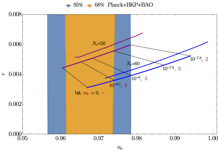
Figure 1: Parametric $(n_{s},r)$ curves as functions of $b\phi$ for $N_{*}=50,60$, with the 68 and 95% CL Planck constraints shown in the background. The solid curves illustrate the parametric dependence using the analytical approximation (38) and (39) assuming $\Delta K=0$. The dashed curves show the power spectrum parameters calculated numerically with $x=-1$, for the same range of $b\phi$. The dotted curves illustrate particular values of $b\phi$, quantified in units of $M_{P}$, and we indicate the corresponding left-handed neutrino masses in units of $10^{-4}$ eV assuming $f_{\nu}\sin\beta=10^{-5}$ and $m=10^{-5}M_{P}$. See Section 4 for more details of the relation between the light neutrino masses and $b\phi$.

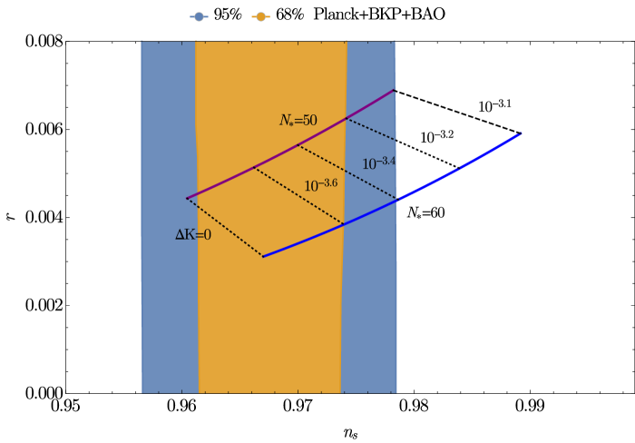
Figure 2: As in Figure 1, but for different values of $\Delta K\equiv|p|^{2}+3|a|^{2}+6|\omega|^{2}+2|\phi|^{2}$, assuming $b\phi=0$.

We see in Fig. 1 the effect of a non-zero value of $b$. The solid curves show the positions in the $(n_{s},r)$ plane for $N_{*}=50$ and 60  as $b\phi$ is increased from 0 to $10^{-7.8}$ using the analytical approximation for the potential given by Eqs. (38) and (39). Here we have taken $\Delta K=0$, and recall that $b\phi=0$ corresponds to the exact Starobinsky result. The dashed lines are derived from a full numerical evolution. For these solutions, $\Delta K\approx 10^{-3.7}$ as would be obtained for $x=-1$. This is the cause of the offset when $b\phi=0$. In order to obtain values of $(n_{s},r)$ consistent with Planck, we must require that the product $b\phi<10^{-7.8}$ $(10^{-8})$ for $N_{*}\simeq 50$ $(60)$ $e$-folds of inflation. Since the vev of $\Phi$ is no larger than the GUT scale, $\phi\lower 3.01385pt\hbox{$\;\stackrel{{\scriptstyle\textstyle<}}{{\sim}}\;$}10^{-2.3}$, the most severe constraint we have on the coupling $b$ is $b<10^{-5.7}$. The scalar potential for several choices of $b\phi$ is shown in Fig. 3. As one can see, so long as $b\phi\lower 3.01385pt\hbox{$\;\stackrel{{\scriptstyle\textstyle<}}{{\sim}}\;$}10^{-2.5}m\sim 10^{-7.5}$, the potential is indistinguishable from the Starobinsky potential out to the value $s\sim 5.5$ needed for 60 $e$-folds of inflation.

Figure 3: The inflationary potential for different values of $b\phi$, in units of the inflaton mass $m\simeq 10^{-5}M_{P}$. The curve labeled $b\phi=0$ is the Starobinsky potential. We assume $\Delta K=0$ here.

We see in Fig. 2 the corresponding effect of varying $\Delta K$ for $b\phi=0$. As we have fixed the value of $\Delta K$, we show here only the analytic result. In this case, in order to obtain values of $(n_{s},r)$ consistent with Planck, we must require that the quantity $\Delta K<10^{-3.1}$ $(10^{-3.4})$ for $N_{*}\simeq 50$ $(60)$ $e$-folds of inflation. If the largest vevs associated with $p,a$ and/or $\omega$ are of order $10^{16}$ GeV, $\Delta K\lower 3.01385pt\hbox{$\;\stackrel{{\scriptstyle\textstyle<}}{{\sim}}\;$}10^{-3.7}$ and the bounds from Planck are always satisfied. The scalar potential for this case is shown by the dashed curve in Fig. 4, and is Starobinsky-like out to $s\approx 8$. Figure 4 also shows the potential for other choices of $\Delta K$ for $b=0$.

For generic values of $b$ and $\Delta K$, we can approximate numerically the limits on $\Delta K$ and $b\phi$ by

$$\Delta K+(2\times 10^{6}\,b\phi)^{2}\leq\begin{cases}0.00078,&N_{*}=50\,,\\ 0.00043,&N_{*}=60\,.\end{cases}$$ (43)

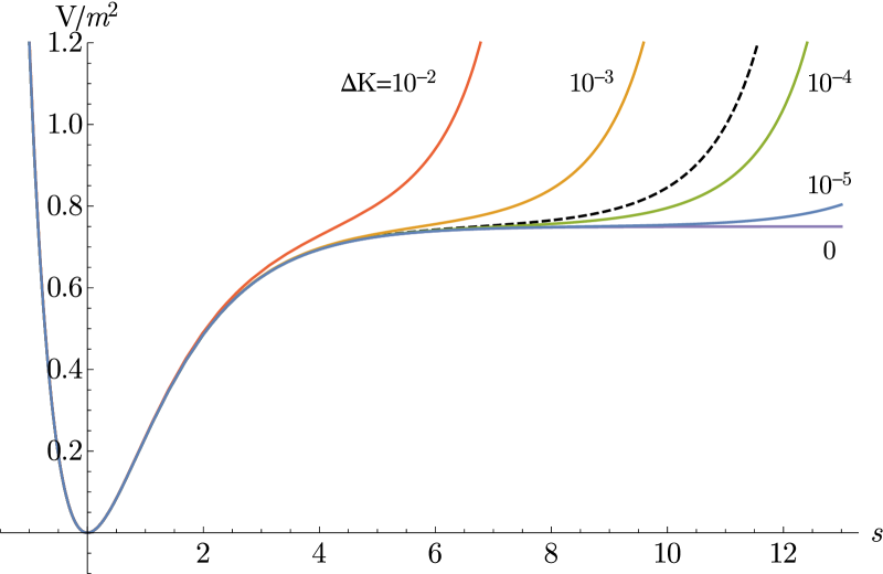
Figure 4: The inflationary potential for different values of $\Delta K\equiv|p|^{2}+3|a|^{2}+6|\omega|^{2}+2|\phi|^{2}$, for $b=0$. The black dashed line corresponds to $\phi=p=a=\omega=10^{16}\,{\rm GeV}$.

So far we have relied on the assumption that the Higgs fields track the instantaneous minimum during inflation. We have verified this behavior by integrating numerically the classical equations of motion, given by

$$\ddot{\Psi}^{a}+3H\dot{\Psi}^{a}+\Gamma^{a}_{bc}\dot{\Psi}^{b}\dot{\Psi}^{c}+K^{a\bar{b}}\frac{\partial V}{\partial\bar{\Psi}^{\bar{b}}}\;=\;0\,.$$ (44)

Here the indices run over all field components, with $\Psi^{a}\equiv\{T,S,p,a,\omega,\phi_{R},\cdots\}$, $K^{a\bar{b}}$ denotes the inverse Kähler metric, and the connection coefficients are given by

$$\Gamma^{a}_{bc}=K^{a\bar{d}}\partial_{b}K_{c\bar{d}}\,.$$ (45)

We consider two types of solutions: 1) $x=-1$ and $\phi=p=a=\omega=M_{\rm GUT}$; 2) $x\simeq 0$ and $\phi<p,a,\omega$, i.e., $M_{\rm int}<M_{\rm GUT}$. As was discussed previously, for case 1) the differences between the instantaneous values of the Higgs fields during inflation and their vacuum vevs are negligibly small, and inflation can be realized for a wide range of values of $b\ll 1$. Fig. 5 displays the numerical solutions for the SM singlets $s$, $\phi$, $p$, $a$, $\omega$ during inflation, for the following set of parameters:

$$m=10^{-5}\,,\quad m_{\Phi}=3.3\times 10^{-2}\,,\quad m_{\Sigma}=8.2\times 10^{-4}\,,\quad\Lambda=-0.2\,,\quad\eta=0.8\,,\quad b=10^{-6}\,,$$ (46)

with $c=\gamma=0$. These parameter values are chosen to obtain vevs for the singlet components of the 210 and 16 ($\overline{\bf 16}$) equal to $10^{16}\,{\rm GeV}$. The resulting inflationary parameters are illustrated in Fig. 1 in the range $0\leq b\leq 3.8\times 10^{-6}$. As one can see the evolution of all fields track very smoothly their local minimum as $s$ evolves over the last $\sim 60$ $e$-folds of inflation. At the end of inflation, all fields begin oscillations about the low energy vacuum.

As an example of case 2), we consider $x=0.0004$. In this case, as discussed at the beginning of this Section, we find that the instantaneous minimum during inflation is displaced relative to its position at $S=0$ by $\delta(p,a,\omega)\propto 10^{-2}b^{2}/x\eta m_{\Phi}$ and $\delta\phi\propto 10^{-2}m_{\Sigma}^{1/2}b^{2}/\eta(xm_{\Phi})^{3/2}$. If $x$ is too small, this deviation can no longer be considered a perturbation, and it can be shown numerically that the Higgs fields are driven towards $\phi=0$, $p=a=\omega$, thus eventually rolling into a ${\rm SU}(5)\otimes{\rm U}(1)$-preserving minimum [51]. Fig. 6 illustrates a particular realization of the hierarchy $\langle\Phi\rangle\ll\langle\Sigma\rangle$ that leads successfully to the SM vacuum. In this case, the parameters used correspond to $\eta=\Lambda=0$, $m_{\Sigma}=4\times 10^{-4}$, $m_{\Phi}=10^{-3}$ and $b=10^{-6}$. The vevs in turn correspond to $a\simeq-10^{16}\,{\rm GeV}$, $\phi\simeq 3\times 10^{14}\,{\rm GeV}$ and $\omega\simeq-p\simeq 4\times 10^{12}\,{\rm GeV}$. In this particular case, the Higgs excursions during inflation are not negligible, which implies that the inflationary potential does not have the simple form (35), and a numerical approach must be followed to constrain the value of $|b\phi|$ that would lead to Planck-compatible inflation. Nevertheless, as Fig. 6 demonstrates, the bound on $|b\phi|$ does not differ significantly from the analytical approximation based on Eq. (39). A smaller value of $x$ would in principle drive the intermediate scale vev lower, but it can be shown numerically that in this case the Higgs fields fail to lead to a SM minimum if we choose a smaller $x$ for any $b\gtrsim 10^{-6}$. We also note in passing that solutions with small $x$ may be problematic for proton decay as we discussed above.

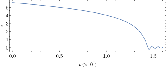
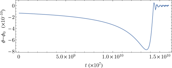
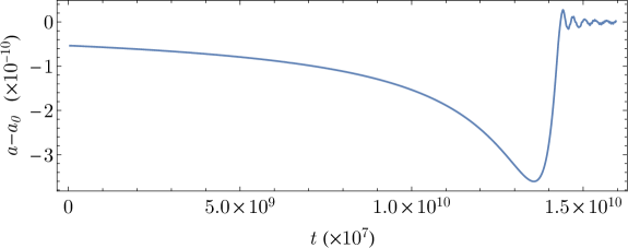
Figure 5: Evolution of the canonically-normalized inflaton $s$ and the SM singlets $\phi,p,a,\omega$ during inflation, for the parameters (46) and $x=-1$. The Higgs vevs $\{p_{0},a_{o},\omega_{0},\phi_{0}\}$ are all equal to $10^{16}\,{\rm GeV}$. For simplicity we display values in Planck units with $M_{P}=1$.

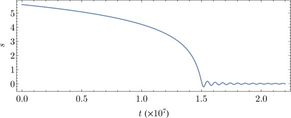
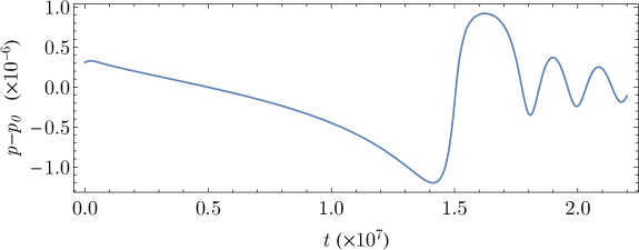
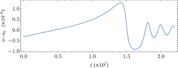
Figure 6: Evolution of the canonically-normalized inflaton $s$ and the SM singlets $\phi,p,a,\omega$ during inflation, for $x=0.0004$. The Higgs vevs are given by $a\simeq-4\times 10^{-3}$, $\phi\simeq 1.1\times 10^{-4}$ and $\omega\simeq-p\simeq 1.6\times 10^{-6}$ in units with $M_{P}=1$.

The initial conditions for the Higgs fields chosen for the numerical solution shown in Figs. 5 and 6 coincide with the position of the instantaneous minimum, but we have checked that inflation and the successive evolution towards the GUT-breaking vacuum are stable if the initial conditions are perturbed by up to $\Delta\phi/\phi_{0}\lesssim{\rm few}\times 10^{-1}$. This is illustrated in Fig. 7 for an initial deviation $\Delta\phi/\phi_{0}=0.2$ for case 1 with $x=-1$. We note that the initial uphill rolling of the inflaton is seeded by the kinetic energy of the oscillations of the Higgs fields through the connection-dependent terms in (44), namely:

$$\Gamma^{S}_{bc}\dot{\Psi}^{b}\dot{\Psi}^{c}\simeq-\frac{1}{2\sqrt{3}}\,\sinh(\sqrt{2/3}\,s)\left(\dot{p}^{2}+2\dot{a}^{2}+6\dot{\omega}^{2}+2\dot{\phi}^{2}\right)+\cdots\,.$$ (47)

As the value of $s$ increases, the oscillations of $\phi$ are rapidly damped, and the subsequent evolution resembles that shown in Fig. 5. Note the difference in timescale in this figure. The transient growth in $s$ implies an increased total number of $e$-folds compared to an unperturbed initial condition. Similarly, for case 2 we are not required to fine-tune the initial positions of the fields with respect to their minima. However, if these perturbations are initially too large, the subsequent evolution may well take the theory to an SO(10)-symmetric vacuum.

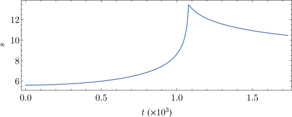
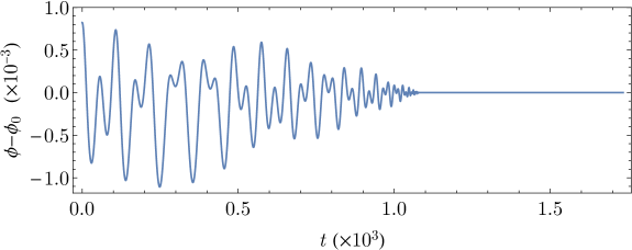
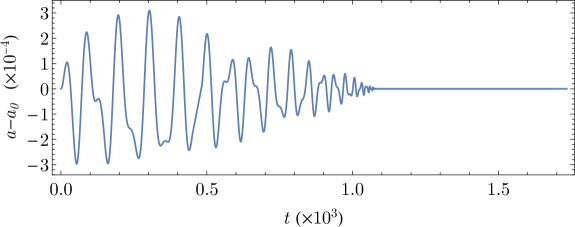
Figure 7: Evolution of the canonically-normalized inflaton $s$ and the SM singlets $\phi,p,a,\omega$ during inflation, for the set of parameters defined by $x=-1$. Here we consider a perturbed initial condition $\Delta\phi/\phi_{0}=0.2$. Here $\{p_{0},a_{o},\omega_{0},\phi_{0}\}$ are as in Fig. 6.

So far we have neglected the effects of the couplings $c$ and $\gamma$, which are not independent as they satisfy the relation (19). Let us for simplicity assume that $c\ll 1$ and $b=0$. In this case, for $s\gg 1$, the Higgs singlet components are displaced from their vevs during inflation by corrections that depend linearly on $c$; for example,

$$\delta\phi\simeq\frac{c}{\eta}\left(\frac{m_{\Sigma}}{m_{\Phi}}\right)^{1/2}\,g(x)\,,$$ (48)

where $g(x)$ is another (somewhat complicated and long) function of $x$. Similarly to the $b\neq 0$, $c=0$ case, the function $g(x)$ is divergent for $x=0,1/3$ and $\pm i$, implying that $\phi$ will be always driven to zero for $x$ close to these points. For any $x$, with a sufficiently large $c$, the corrections will be large due to the induced mass-squared $\sim(cS)^{2}$, and all Higgs singlets will be driven to zero during inflation, leaving the universe in an SO(10)-symmetric state. In the particular case with $x=-1$ and $\phi=p=a=\omega=10^{16}\,{\rm GeV}$, this occurs for $c\gtrsim 3\times 10^{-3}$.

As the analytic approximation (36) is valid for very small $c$, one would be tempted to relate directly the Planck constraint on $|b\phi|$ with a constraint on the combination $2|c\phi|^{2}+|2\gamma p|^{2}+|6\gamma a|^{2}+|12\gamma\omega|^{2}$. However, it can be verified numerically that values of $c$ larger than the value that one would naively have expected to be the maximum compatible with Planck data can still lead to Planck-compatible results; the deviations of the fields with respect to their vevs compensate the expected deformation of the inflaton potential. For example, in the previously-discussed $x=-1$ case, the naive expectation would result in the bound $c\lesssim 5\times 10^{-7}$, whereas a numerical calculation shows that 95% Planck compatibility is retained for $c\lesssim 7\times 10^{-4}$, only a factor of four below the maximum value of $c$ allowed by symmetry breaking.

The specific limits on $b$ and $c$ when both are non-vanishing must be checked numerically on a case-by-case basis. Nevertheless, it is clear that the allowed values of $b$ and $c$ are reduced due to the simultaneous effect of both couplings.

4 Yukawa Couplings and Neutrino Masses

4.1 Yukawa unification and its violation

As discussed in Section 2.2.3, the MSSM Higgs fields $H_{u}$ and $H_{d}$ in our model are given by linear combinations of the SU(2)_L doublet components in the fields $\Phi$, $\bar{\Phi}$, and $H$. The Yukawa coupling terms in the low-energy effective theory are then written as

$$W_{\rm Yukawa}=f_{u}H_{u}Q\bar{u}+f_{\nu}H_{u}L{\nu}^{c}_{R}-f_{d}H_{d}Q\bar{d}-f_{e}H_{d}L\bar{e}~{},$$ (49)

where the Yukawa couplings are related to the corresponding GUT Yukawa couplings through the following GUT-scale matching conditions:

$$f_{u}=f_{\nu}=y\,{\cal U}_{11}~{},~{}~{}~{}~{}~{}~{}f_{d}=f_{e}=y{\cal D}_{11}~{}.$$ (50)

These equations show that we expect the unification of down-type quark and charged-lepton Yukawa couplings at the GUT scale, as in SU(5) GUTs, and the up-type quark and neutrino Yukawa couplings are also unified. These two classes of the Yukawa couplings may, however, be different from each other if $\alpha\neq\bar{\alpha}$, since ${\cal U}_{11}\neq{\cal D}_{11}$ in this case. This feature distinguishes our model from other SO(10) GUT models, where one usually has $f_{u}=f_{d}=f_{e}=f_{\nu}$ at the GUT scale.

These GUT relations are modified if there exist higher-dimensional operators suppressed by the Planck scale [69]. Among such operators, the following dimension-five operator is expected to give the leading contribution:

$$W_{\rm eff}=\frac{c_{\Delta f}}{M_{P}}H\Sigma\psi\psi~{}.$$ (51)

After $\Sigma$ develops a vev, this operator leads to the Yukawa couplings in Eq. (49). The matching conditions in this case are given by

$$f_{u} =(y+\Delta f)\,{\cal U}_{11}~{},~{}~{}~{}~{}~{}~{}f_{\nu}=(y-3\Delta f)\,{\cal U}_{11}~{},$$

$$f_{d} =(y+\Delta f)\,{\cal D}_{11}~{},~{}~{}~{}~{}~{}~{}f_{e}=(y-3\Delta f)\,{\cal D}_{11}~{},$$ (52)

with

$$\Delta f=\frac{c_{\Delta f}}{M_{P}}(a+\omega)~{}.$$ (53)

Since $\Delta f={\cal O}(10^{-3})$ for $c_{\Delta f}={\cal O}(1)$, the GUT relations for the first- and second-generation Yukawa couplings may be modified significantly in the presence of the dimension-five operator. For the third-generation Yukawa couplings, on the other hand, its effects are less significant. Intriguingly, this is consistent with the observed quark and lepton mass spectrum; experimentally, bottom and tau Yukawa unification is realized at the ${\cal O}(10)$% level in most of the parameter space in the MSSM , while the deviations in $s$-$\mu$ and $d$-$e$ unification are as large as ${\cal O}(100)$%.

4.2 Neutrino masses

We now investigate the mass matrix for neutrinos. If we take $M,b^{\prime},\alpha^{\prime}\to 0$, then $\Phi$ and $\bar{\Phi}$ have no mixing with neutrinos; we consider this limit for simplicity. Note that this limit suppresses the $R$-parity violating operators, and thus is phenomenologically desirable as we discuss below. A non-zero value of the coupling $b$ induces mixing between right-handed neutrinos and the singlinos $\tilde{S}_{i}$, which are the fermionic component of the singlet superfields $S_{i}$. We also suppress the couplings $c$, $\gamma$, and $\lambda_{SH}$ in order to prevent $S$ from mixing with $\Phi$, $\bar{\Phi}$, $\Sigma$, and $H$. As we have seen above, for the inflaton field, the smallness of $c$ and $\gamma$ is required by successful inflation, while $\lambda_{SH}$ should be small in order to avoid over-production of gravitinos as we will see in the next section. In this case, mixing occurs only among the right- and left-handed neutrinos and the singlinos. Disregarding Planck-suppressed factors, the neutrino-singlino fermion mass matrix takes the form [43]

$${\cal L}_{\rm mass}=-\begin{pmatrix}\overline{\nu}_{L}&\overline{\nu}^{c}_{R}&\overline{\tilde{S}}\end{pmatrix}\begin{pmatrix}0&-f_{\nu}\,v\sin\beta&0\\ -f_{\nu}\,v\sin\beta&0&-b\phi\\ 0&-b\phi&m\end{pmatrix}\begin{pmatrix}\nu_{L}\\[3.0pt] \nu_{R}^{c}\\[3.0pt] \tilde{S}\end{pmatrix}\,,$$ (54)

where $v\simeq 174$ GeV is the Standard Model Higgs vev and $\tan\beta\equiv\langle H_{u}\rangle/\langle H_{d}\rangle$. A similar form for the mass matrix is found in flipped SU(5) [56, 70].

For the first-generation neutrinos, the requirement of successful inflation restricts the coupling $b$ as we have seen in the previous section. In this case, the couplings satisfy the hierarchy

$$f_{\nu}\,v\sin\beta\ll b\phi\ll m~{},$$ (55)

and thus the diagonal mass matrix has a double-seesaw form given approximately by

$${\cal L}_{\rm mass}=-\begin{pmatrix}\overline{\nu}_{L}^{M}&\overline{\nu}_{R}^{M}&\overline{\tilde{S}}^{M}\end{pmatrix}\begin{pmatrix}m\left(\frac{f_{\nu}\,v\sin\beta}{b\phi}\right)^{2}&0&0\\ 0&-\frac{(b\phi)^{2}}{m}-m\left(\frac{f_{\nu}\,v\sin\beta}{b\phi}\right)^{2}&0\\ 0&0&m+\frac{(b\phi)^{2}}{m}\end{pmatrix}\begin{pmatrix}\nu_{L}^{M}\\[5.0pt] \nu_{R}^{M}\\[5.0pt] \tilde{S}^{M}\end{pmatrix}\,,$$ (56)

and the corresponding mass eigenstates are approximately

$$\nu_{L}^{M}\; \simeq\;\nu_{L}\,-\,\frac{m\,f_{\nu}v\sin\beta}{(b\phi)^{2}}\,\nu_{R}^{c}\,-\,\frac{f_{\nu}v\sin\beta}{b\phi}\,\tilde{S}\,,$$ (57)

$$\nu_{R}^{M}\; \simeq\;\nu_{R}^{c}\,+\,\frac{b\phi}{m}\,\tilde{S}\,+\,\frac{m\,f_{\nu}v\sin\beta}{(b\phi)^{2}}\,\nu_{L}\,,$$ (58)

$$\tilde{S}^{M}\; \simeq\;\tilde{S}\,-\,\frac{b\phi}{m}\,\nu_{R}^{c}\,+\,\frac{b\phi\,f_{\nu}v\sin\beta}{m^{2}}\,\nu_{L}\,.$$ (59)

For the second and third generations, on the other hand, the coupling $b$ (recall we have suppressed all generation indices) can be arbitrary, but the masses for light neutrinos are still given by

$$m_{\nu}\simeq m\left(\frac{f_{\nu}\,v\sin\beta}{b\phi}\right)^{2}~{}.$$ (60)

Figure 8: The neutrino mass spectrum in the double-seesaw scenario arising from (54), assuming $m=10^{-5}M_{P}$ and $f_{\nu}\sin\beta=2\times 10^{-5}$, as a function of $b\phi$. For these parameters, the allowed range for $b\phi$ and correspondingly the neutrino masses, is located in the upper left region, bounded to the left by the vertical dashed line showing the 95% CL Planck upper limit $b\phi=10^{-7.8}M_{P}$, and below by the horizontal dashed line corresponding to $m_{L}\simeq 2\times 10^{-13}\,{\rm GeV}.$

Values of the mass eigenvalues calculated numerically for $m\simeq 10^{-5}M_{P}$ are shown in Fig. 8. If $b\phi\sim 10^{-8.5}M_{P}$, a left-handed neutrino mass $m_{L}\lesssim 0.1\,{\rm eV}$ is obtained if $f_{\nu}\sin\beta\lesssim 9\times 10^{-5}$ . Currently, the Planck 2015 data [1] imposes a constraint on the sum of the neutrino masses: $\sum m_{\nu}<0.23$ eV, and an even stronger bound of $\sum m_{\nu}<0.12$ eV comes from the Lyman $\alpha$ forest power spectrum obtained by BOSS in combination with CMB data [72]. Since the parameters $b$ and $m$ for the second and third generations are almost arbitrary, we may explain the current neutrino oscillation data [73] by appropriately choosing these parameters (as well as flavor-changing couplings corresponding to $b$ and $m$). For $f_{\nu}\sin\beta=m_{u}/v$ and $m=10^{-5}$, the normal hierarchical neutrino mass spectrum is obtained if $b\phi\gg 10^{-9}$. On the other hand, the neutrino mass spectrum is inverted if $b\phi\simeq 7\times 10^{-10}$. A smaller value of $b\phi$ leads to a quasi-degenerate mass spectrum. The latter two types of mass spectrum are constrained by both neutrino oscillation data [73] and the CMB observations [1, 72], and will be tested in future experiments. It has not escaped our attention that there is a strong correlation between the CMB observations, as quantified in the values of $n_{s}$ and $r$, and the light neutrino masses, that becomes apparent if we write (41) and (42) as

$$n_{s} \;\simeq\;-\frac{2}{N_{*}}+\frac{8}{3}\left(\frac{m}{m_{\nu}}\right)\left(\frac{f_{\nu}\,v\sin\beta}{m}\right)^{2}N_{*}^{2}+\frac{32}{81}\,\Delta K\,N_{*}\,,$$ (61)

$$r \;\simeq\;\frac{12}{N_{*}^{2}}+\frac{32}{3}\left(\frac{m}{m_{\nu}}\right)\left(\frac{f_{\nu}\,v\sin\beta}{m}\right)^{2}N_{*}+\frac{64}{27}\,\Delta K\,.$$ (62)

When the couplings $M$ and $b^{\prime}$ are different from zero (and related by the minimization condition (20)), the fermion mass matrix for the SM singlets and uncharged doublets ceases to be block-diagonal, and potentially large terms such as $\mathcal{M}^{\nu_{L}\bar{\phi}_{L}}=M+b^{\prime}(p-3a)$ or $\mathcal{M}^{\nu_{R}\,p}=b^{\prime}\phi$ will in general result in significantly mixed mass eigenstates. As a crude approximation, if one assumes that only the ‘left-handed’ fields mix, i.e., the fermionic components of $H_{L},\bar{H}_{L},\phi_{L},\bar{\phi}_{L}$ together with $\nu_{L}$, one can compute, e.g., the contribution of the $\tilde{\phi}_{L}$ gauge eigenstate to the lightest state, which in the $b^{\prime}\rightarrow 0$ limit would correspond to a pure $\nu_{L}$ state. This contribution has the form

$$\psi_{\rm lightest}^{(\phi_{L})}\simeq\frac{m_{H}}{\Delta}(M+b^{\prime}(p-3a))\,,$$ (63)

where $\Delta\ll M_{\rm GUT}^{2}$ has been defined in (28), and is related to the weak-scale $\mu$-term via $\Delta\simeq\mu\,[m_{H}+2\eta(p+3\omega)]$. This implies that sizable mixing can occur for $b^{\prime}\gtrsim\mu/M_{\rm GUT}$. For a larger $b^{\prime}$ (and thus $M$), the fine-tuning condition for the doublet-triplet splitting is modified, and it turns out that $\Delta$ should also grow ($\Delta\propto b^{\prime}$ for $b^{\prime}\gg\mu/M_{\rm GUT}$) to keep $\mu$ at the supersymmetry-breaking scale. In any case, as we see in the subsequent section, we need to $b^{\prime},M$ to be small in order to ensure a good dark matter candidate (the lightest neutralino with a lifetime longer than the age of the Universe), and thus we do not consider further in this paper the case of large $b^{\prime},M$.

As discussed previously, non-vanishing values of $c$ and $\gamma$ would mix the Higgs sector and the inflatino $\tilde{S}$. However, we have verified that, in the Planck-allowed range for $c$, the mass spectrum, and in particular the left-handed neutrino state, are negligibly affected.

5 Reheating and Leptogenesis

In the absence of a direct coupling between the inflaton and matter, reheating in supergravity models almost always proceeds through the minimal gravitational couplings [74], leading to a minimal reheat temperature of order $10^{6}$ GeV [75]. However, these couplings vanish in no-scale supergravity [37] and reheating must proceed either though a direct coupling to matter or a coupling to gauge fields through the gauge kinetic term. For this reason, the identification of the inflaton with the right-handed sneutrino has appeared to be very promising, as reheating takes place naturally through the decays of the inflaton to sneutrino/Higgs or neutrino/Higgsino pairs [24, 27]. In fact, to avoid excessive reheating and gravitino production, it was necessary to set a limit on Yukawa coupling of the inflaton (right-handed sneutrino) of order $10^{-5}$, comparable to the electron Yukawa coupling.

In the present context, the inflaton is once again a singlet, and the coupling $b$ yields the direct coupling of the inflaton to Standard Model matter fields through the $\bar{\Phi}$-$H$ and neutrino-singlino mixings. For the former, the $bS\bar{\Phi}\psi$ term leads to $b\,{\cal U}_{21}SH_{u}L$ via the mixing (29). For the latter, the neutrino Yukawa coupling $f_{\nu}$ induces an inflaton-Higgs-neutrino coupling through the scalar mixing

$$\tilde{\nu}_{R} \simeq\tilde{\nu}_{R}^{M}-\frac{b\phi}{m}\,S^{M}\,,$$ (64)

$$S \simeq S^{M}+\frac{b\phi}{m}\,\tilde{\nu}_{R}^{M}\,,$$ (65)

where we have disregarded weak-scale terms, cf., Eqs. (57–59). As a result, we obtain an interaction

$${\cal L}_{\rm int}=-C_{SHL}\,S^{M}H_{u}L~{},$$ (66)

with

$$C_{SHL}=b\left({\cal U}_{21}-\frac{f_{\nu}\phi}{m}\right)~{}.$$ (67)

This results in the inflaton decay rate

$$\Gamma(S\rightarrow H_{u}\tilde{L})+\Gamma(S\rightarrow\tilde{H}_{u}L)=\frac{m}{4\pi}\left|C_{SHL}\right|^{2}\,,$$ (68)

which leads to a reheat temperature

$$T_{R}\simeq 10^{15}~{}{\rm GeV}\times\left|C_{SHL}\right|\left(\frac{g_{*}}{915/4}\right)^{-1/4}\left(\frac{m}{10^{-5}M_{P}}\right)^{1/2}~{},$$ (69)

where $g_{*}$ denotes the effective number of degrees of freedom, and $g_{*}=915/4$ for the MSSM.

The abundance of gravitinos is determined by the reheat temperature [76]:

$$\frac{n_{3/2}}{s}\simeq 2.4\times 10^{-12}\left(\frac{T_{R}}{10^{10}~{}{\rm GeV}}\right)\,,$$ (70)

where $s$ is the entropy density and we have assumed that the gravitino is much heavier than the gluino. In order to satisfy the upper limit on the abundance of neutralinos: $\Omega_{\chi}h^{2}<0.12$, we must ensure that [77]

$$\frac{n_{3/2}}{s}\lesssim 4.4\times 10^{-13}\left(\frac{1{\rm TeV}}{m_{\chi}}\right)\,,$$ (71)

which leads to an upper limit on the coupling $C_{SHL}$:

$$\left|C_{SHL}\right|\lesssim 10^{-5}\,.$$ (72)

Since we expect ${\cal U}_{21}={\cal O}(1)$, $f_{\nu}={\cal O}(10^{-5})$, and $m/\phi={\cal O}(10^{-3})$ in our setup, this bound implies $|C_{SHL}|\sim|b|\lesssim 10^{-5}$. For a more detailed discussion of reheating, see [78].

If $\lambda_{SH}\neq 0$, the inflaton can decay into a pair of higgsinos as well. Similarly to the above case, to evade over-production of gravitinos, we need to suppress this coupling such that $|\lambda_{SH}|\lesssim 10^{-5}$.

As noted earlier, $R$-parity is violated in this model though, as described in [24], the violation via the coupling $b$ is weak enough to ensure that the lifetime of the lightest supersymmetric particle is much longer than the age of the Universe. To stabilize the lightest supersymmetric particle, we need to take $\alpha^{\prime}$, $M$ and $b^{\prime}$ to be zero since they make it decay at tree level. The form of the coupling of $S$ in Eq. (66) is clearly an $L$-violating decay, so the reheating process may well lead to a lepton asymmetry given by [79, 74]

$$\frac{n_{L}}{s}\sim\epsilon\frac{n_{S}}{T_{R}^{3}}\sim\epsilon\frac{T_{R}}{m}\,,$$ (73)

where $n_{S}$ is the number density of inflatons at the time of their decay. This lepton (or $B-L$) asymmetry then generates a baryon asymmetry [80, 81] through sphaleron interactions [82, 83]. The factor $\epsilon$ is a measure of the C and CP violation in the decay, which is determined by loops in which one or both of the remaining singlet states is exchanged, and is given by [84]

$$\epsilon\simeq-\frac{3}{8\pi}\frac{1}{\left(C_{SHL}C_{SHL}^{\dagger}\right)_{11}}\sum_{i=2,3}{\rm Im}\left[\left(C_{SHL}C_{SHL}^{\dagger}\right)^{2}_{1i}\right]\frac{M_{1}}{M_{i}}~{},$$ (74)

where $M_{1}=m\ll M_{2},M_{3}$ are the masses of the singlets, where the lightest is assumed to be the inflaton . In order to obtain the correct baryon asymmetry, we should place additional constraints on the couplings and masses of the heavier singlets, which we do not discuss further here.

6 Summary

It has been shown previously that no-scale supergravity with bilinear and trilinear self-couplings of a singlet inflaton field provides an economical way to realize a model of inflation whose predictions for the inflationary observables $(n_{s},r)$ are similar to those of the Starobinsky model. In this paper we have studied how this scenario may be embedded in a supersymmetric GUT that is able to address other interesting phenomenological issues such as fermion (particularly neutrino) masses, proton decay, leptogenesis, gravitino production and the nature of dark matter.

In this paper we have addressed these issues in a supersymmetric SO(10) GUT model. In general, sneutrino inflation is an attractive scenario, but this cannot be realized in an SO(10) GUT, because sneutrinos are embedded in matter $\mathbf{16}$ representations of SO(10), but there are no $\mathbf{16}^{2}$ or $\mathbf{16}^{3}$ couplings in SO(10). We therefore consider an SO(10) GUT model with a singlet inflaton field, in which there is an intermediate stage of symmetry breaking provided by a Higgs $\mathbf{16}$ multiplet. This model has the Kähler potential shown in (10) and the superpotential shown in (9). As discussed in Section 2, we consider various possible patterns of symmetry breaking, paying careful attention to the vacuum conditions in each case.

We have shown that inflation can be realized in such a framework, studying numerically the behaviours of the scalar fields during the inflationary epoch. In particular, we tracked the evolution of the the three Standard Model singlets in the 210 responsible for breaking SO(10), the single in the Higgs 16 simultaneously with the inflaton. One of the important phenomenological issues in constructing such a GUT model is doublet-triplet mass splitting. As we have discussed, the proton stability constraint requires either a very high supersymmetry-braking scale and/or some additional mechanism to suppress the color-triplet Higgs exchange contribution. These issues may be more easily resolved in a flipped ${\rm SU}(5)\otimes{\rm U}(1)$ model [56] where the Higgs structure is greatly simplified (only a 10, $\mathbf{\overline{10}}$, 5, $\mathbf{\bar{5}}$ of Higgses are needed instead of the 210, 16, and $\mathbf{\overline{16}}$ considered here).

We have discussed the fermion masses in this model, point out that it predicts the (phenomenologically successful) unification of the $b$ and $\tau$ Yukawa couplings, and similar unification between the Yukawa couplings in the up-type quark and neutrino sectors. The neutrino masses have a double-seesaw structure involving the left- and right-handed neutrinos and the singlino partner of the inflaton field. We have explored the constraints that neutrino masses impose on this structure, and shown that it can lead to successful leptogenesis.

Two specifically supersymmetric issues are gravitino production during reheating at the end of inflation and the nature of dark matter. Avoiding the overproduction of gravitinos imposes a reasonable constraint on the inflaton Yukawa coupling, which should be at most comparable to that of the electron. In this model $R$ parity is not conserved, so one might fear for the stability of supersymmetric dark matter. However, the lifetime of the lightest supersymmetric particle is typically much longer than the age of the Universe, so this is still a plausible candidate for dark matter.

The no-scale SO(10) GUT scenario for inflation described here has many attractive features, since it combines Starobinsky-like predictions for the inflationary perturbations with many phenomenological desiderata. We therefore consider it a significant step forward in inflationary model-building, while admitting that it has some issues, notably proton stability. Thus there is still significant scope for further improvement.

References

- [1] P. A. R. Ade et al. [Planck Collaboration], arXiv:1502.01589 [astro-ph.CO]; P. A. R. Ade et al. [Planck Collaboration], arXiv:1502.02114 [astro-ph.CO].
- [2] P. A. R. Ade et al. [BICEP2 and Planck Collaborations], Phys. Rev. Lett. 114, no. 10, 101301 (2015) [arXiv:1502.00612 [astro-ph.CO]].
- [3] J. Martin, C. Ringeval and V. Vennin, Phys. Dark Univ. 5-6, 75-235 (2014) [arXiv:1303.3787 [astro-ph.CO]]; J. Martin, C. Ringeval, R. Trotta and V. Vennin, JCAP 1403 (2014) 039 [arXiv:1312.3529 [astro-ph.CO]]; J. Martin, arXiv:1502.05733 [astro-ph.CO].
- [4] A. A. Starobinsky, Phys. Lett. B 91, 99 (1980).
- [5] V. F. Mukhanov and G. V. Chibisov, JETP Lett. 33, 532 (1981) [Pisma Zh. Eksp. Teor. Fiz. 33, 549 (1981)].
- [6] A. A. Starobinsky, Sov. Astron. Lett. 9, 302 (1983).
- [7] F. L. Bezrukov and M. Shaposhnikov, Phys. Lett. B 659, 703 (2008) [arXiv:0710.3755 [hep-th]].
- [8] D. Buttazzo, G. Degrassi, P. P. Giardino, G. F. Giudice, F. Sala, A. Salvio and A. Strumia, JHEP 1312 (2013) 089 [arXiv:1307.3536].
- [9] J. R. Ellis, D. V. Nanopoulos, K. A. Olive and K. Tamvakis, Phys. Lett. B 118 (1982) 335; Phys. Lett. B 120 (1983) 331; Nucl. Phys. B 221 (1983) 52; K. Nakayama and F. Takahashi, JCAP 1110, 033 (2011) [arXiv:1108.0070 [hep-ph]].
- [10] D. V. Nanopoulos, K. A. Olive, M. Srednicki and K. Tamvakis, Phys. Lett. B 123, 41 (1983); D. V. Nanopoulos, K. A. Olive and M. Srednicki, Phys. Lett. B 127, 30 (1983).
- [11] R. Holman, P. Ramond and G. G. Ross, Phys. Lett. B 137, 343 (1984).
- [12] A. B. Goncharov and A. D. Linde, Phys. Lett. B 139, 27 (1984).
- [13] E. J. Copeland, A. R. Liddle, D. H. Lyth, E. D. Stewart and D. Wands, Phys. Rev. D 49, 6410 (1994) [astro-ph/9401011]; E. D. Stewart, Phys. Rev. D 51, 6847 (1995) [hep-ph/9405389].
- [14] E. Cremmer, S. Ferrara, C. Kounnas and D. V. Nanopoulos, Phys. Lett. B 133 (1983) 61; J. R. Ellis, A. B. Lahanas, D. V. Nanopoulos and K. Tamvakis, Phys. Lett. B 134 (1984) 429.
- [15] A. B. Lahanas and D. V. Nanopoulos, Phys. Rept. 145 (1987) 1.
- [16] E. Witten, Phys. Lett. B 155 (1985) 151.
- [17] M. K. Gaillard, H. Murayama and K. A. Olive, Phys. Lett. B 355 (1995) 71 [hep-ph/9504307].
- [18] A. S. Goncharov and A. D. Linde, Class. Quant. Grav. 1, L75 (1984).
- [19] C. Kounnas and M. Quiros, Phys. Lett. B 151, 189 (1985).
- [20] J. R. Ellis, K. Enqvist, D. V. Nanopoulos, K. A. Olive and M. Srednicki, Phys. Lett. B 152 (1985) 175 [Erratum-ibid. 156B (1985) 452].
- [21] K. Enqvist, D. V. Nanopoulos and M. Quiros, Phys. Lett. B 159, 249 (1985); P. Binétruy and M. K. Gaillard, Phys. Rev. D 34, 3069 (1986); H. Murayama, H. Suzuki, T. Yanagida and J. Yokoyama, Phys. Rev. D 50, 2356 (1994) [arXiv:hep-ph/9311326]; S. C. Davis and M. Postma, JCAP 0803, 015 (2008) [arXiv:0801.4696 [hep-ph]]; S. Antusch, M. Bastero-Gil, K. Dutta, S. F. King and P. M. Kostka, JCAP 0901, 040 (2009) [arXiv:0808.2425 [hep-ph]]; S. Antusch, M. Bastero-Gil, K. Dutta, S. F. King and P. M. Kostka, Phys. Lett. B 679, 428 (2009) [arXiv:0905.0905 [hep-th]]; S. Antusch, K. Dutta, J. Erdmenger and S. Halter, JHEP 1104 (2011) 065 [arXiv:1102.0093 [hep-th]]; R. Kallosh and A. Linde, JCAP 1011, 011 (2010) [arXiv:1008.3375 [hep-th]]; R. Kallosh, A. Linde and T. Rube, Phys. Rev. D 83, 043507 (2011) [arXiv:1011.5945 [hep-th]]; T. Li, Z. Li and D. V. Nanopoulos, JCAP 1402, 028 (2014) [arXiv:1311.6770 [hep-ph]]; W. Buchmuller, C. Wieck and M. W. Winkler, Phys. Lett. B 736, 237 (2014) [arXiv:1404.2275 [hep-th]].
- [22] J. Ellis, D. V. Nanopoulos and K. A. Olive, Phys. Rev. Lett. 111 (2013) 111301 [arXiv:1305.1247 [hep-th]].
- [23] J. Ellis, D. V. Nanopoulos and K. A. Olive, JCAP 1310 (2013) 009 [arXiv:1307.3537 [hep-th]].
- [24] J. Ellis, D. V. Nanopoulos and K. A. Olive, Phys. Rev. D 89, 043502 (2014) [arXiv:1310.4770 [hep-ph]].
- [25] R. Kallosh and A. Linde, JCAP 1306 (2013) 028 [arXiv:1306.3214 [hep-th]].
- [26] T. Li, Z. Li and D. V. Nanopoulos, JCAP 1404, 018 (2014) [arXiv:1310.3331 [hep-ph]]; T. Li, Z. Li and D. V. Nanopoulos, Eur. Phys. J. C 75, no. 2, 55 (2015) [arXiv:1405.0197 [hep-th]]; F. Farakos, A. Kehagias and A. Riotto, Nucl. Phys. B 876, 187 (2013) [arXiv:1307.1137 [hep-th]]; S. Ferrara, R. Kallosh, A. Linde and M. Porrati, Phys. Rev. D 88 (2013) 8, 085038 [arXiv:1307.7696 [hep-th]]; W. Buchmüller, V. Domcke and C. Wieck, Phys. Lett. B 730, 155 (2014) [arXiv:1309.3122 [hep-th]]; C. Pallis, JCAP 1404, 024 (2014) [arXiv:1312.3623 [hep-ph]]; C. Pallis, JCAP 1408, 057 (2014) [arXiv:1403.5486 [hep-ph]]; I. Antoniadis, E. Dudas, S. Ferrara and A. Sagnotti, Phys. Lett. B 733, 32 (2014) [arXiv:1403.3269 [hep-th]]; S. Ferrara, A. Kehagias and A. Riotto, Fortsch. Phys. 62, 573 (2014) [arXiv:1403.5531 [hep-th]]; S. Ferrara, A. Kehagias and A. Riotto, Fortsch. Phys. 63, 2 (2015) [arXiv:1405.2353 [hep-th]]; R. Kallosh, A. Linde, B. Vercnocke and W. Chemissany, JCAP 1407, 053 (2014) [arXiv:1403.7189 [hep-th]]; K. Hamaguchi, T. Moroi and T. Terada, Phys. Lett. B 733, 305 (2014) [arXiv:1403.7521 [hep-ph]]; J. Ellis, M. A. G. García, D. V. Nanopoulos and K. A. Olive, JCAP 1405, 037 (2014) [arXiv:1403.7518 [hep-ph]]; J. Ellis, M. A. G. García, D. V. Nanopoulos and K. A. Olive, JCAP 1408, 044 (2014) [arXiv:1405.0271 [hep-ph]]; J. Ellis, M. A. G. García, D. V. Nanopoulos and K. A. Olive, JCAP 1501, no. 01, 010 (2015) [arXiv:1409.8197 [hep-ph]]; W. Buchmuller, E. Dudas, L. Heurtier and C. Wieck, JHEP 1409, 053 (2014) [arXiv:1407.0253 [hep-th]]; W. Buchmuller, E. Dudas, L. Heurtier, A. Westphal, C. Wieck and M. W. Winkler, JHEP 1504, 058 (2015) [arXiv:1501.05812 [hep-th]]; C. Kounnas, D. Lüst and N. Toumbas, Fortsch. Phys. 63, 12 (2015) [arXiv:1409.7076 [hep-th]]; T. Terada, Y. Watanabe, Y. Yamada and J. Yokoyama, JHEP 1502, 105 (2015) [arXiv:1411.6746 [hep-ph]]; A. B. Lahanas and K. Tamvakis, Phys. Rev. D 91, no. 8, 085001 (2015) [arXiv:1501.06547 [hep-th]]; I. Dalianis and F. Farakos, JCAP 1507, no. 07, 044 (2015) [arXiv:1502.01246 [gr-qc]]. D. Roest and M. Scalisi, Phys. Rev. D 92, 043525 (2015) [arXiv:1503.07909 [hep-th]]. M. Scalisi, JHEP 1512, 134 (2015) [arXiv:1506.01368 [hep-th]].
- [27] J. Ellis, M. A. G. Garcia, D. V. Nanopoulos and K. A. Olive, JCAP 1510, no. 10, 003 (2015) [arXiv:1503.08867 [hep-ph]].
- [28] J. Ellis, M. A. G. Garcia, D. V. Nanopoulos and K. A. Olive, JCAP 1507, no. 07, 050 (2015) [arXiv:1505.06986 [hep-ph]].
- [29] J. Ellis, M. A. G. Garcia, D. V. Nanopoulos and K. A. Olive, Class. Quant. Grav. 33, no. 9, 094001 (2016) [arXiv:1507.02308 [hep-ph]].
- [30] I. Garg and S. Mohanty, Phys. Lett. B 751, 7 (2015) [arXiv:1504.07725 [hep-ph]].
- [31] J. Ellis, H. J. He and Z. Z. Xianyu, Phys. Rev. D 91, no. 2, 021302 (2015) [arXiv:1411.5537 [hep-ph]]; arXiv:1606.02202 [hep-ph].
- [32] J. R. Ellis, C. Kounnas and D. V. Nanopoulos, Nucl. Phys. B 247 (1984) 373.
- [33] D. Croon, J. Ellis and N. E. Mavromatos, Phys. Lett. B 724 (2013) 165 [arXiv:1303.6253 [astro-ph.CO]].
- [34] S. Cecotti, Phys. Lett. B 190 (1987) 86.
- [35] J. R. Ellis, C. Kounnas and D. V. Nanopoulos, Phys. Lett. B 143, 410 (1984).
- [36] J. Ellis, M. A. G. Garcia, D. V. Nanopoulos and K. A. Olive, JCAP 1405 (2014) 037 [arXiv:1403.7518 [hep-ph]].
- [37] M. Endo, K. Kadota, K. A. Olive, F. Takahashi and T. T. Yanagida, JCAP 0702, 018 (2007) [hep-ph/0612263].
- [38] R. Kallosh, A. Linde, K. A. Olive and T. Rube, Phys. Rev. D 84, 083519 (2011) [arXiv:1106.6025 [hep-th]].
- [39] L. Calibbi, Y. Mambrini and S. K. Vempati, JHEP 0709, 081 (2007) [arXiv:0704.3518 [hep-ph]]; L. Calibbi, A. Faccia, A. Masiero and S. K. Vempati, Phys. Rev. D 74, 116002 (2006) [arXiv:hep-ph/0605139]; E. Carquin, J. Ellis, M. E. Gomez, S. Lola and J. Rodriguez-Quintero, JHEP 0905 (2009) 026 [arXiv:0812.4243 [hep-ph]]; J. Ellis, A. Mustafayev and K. A. Olive, Eur. Phys. J. C 69, 201 (2010) [arXiv:1003.3677 [hep-ph]]; J. Ellis, A. Mustafayev and K. A. Olive, Eur. Phys. J. C 69, 219 (2010) [arXiv:1004.5399 [hep-ph]]; J. Ellis, A. Mustafayev and K. A. Olive, Eur. Phys. J. C 71, 1689 (2011) [arXiv:1103.5140 [hep-ph]].
- [40] J. Ellis, J. L. Evans, A. Mustafayev, N. Nagata and K. A. Olive, arXiv:1608.05370 [hep-ph].
- [41] H. Murayama, H. Suzuki, T. Yanagida and J. ’i. Yokoyama, Phys. Rev. Lett. 70, 1912 (1993); J. R. Ellis, M. Raidal and T. Yanagida, Phys. Lett. B 581 (2004) 9 [hep-ph/0303242]; S. Antusch, M. Bastero-Gil, K. Dutta, S. F. King and P. M. Kostka, JCAP 0901, 040 (2009) [arXiv:0808.2425 [hep-ph]].
- [42] H. Georgi, AIP Conf. Proc. 23, 575 (1975); H. Fritzsch and P. Minkowski, Annals Phys. 93, 193 (1975); M. S. Chanowitz, J. R. Ellis and M. K. Gaillard, Nucl. Phys. B 128, 506 (1977).
- [43] H. Georgi and D. V. Nanopoulos, Phys. Lett. B 82, 392 (1979); H. Georgi and D. V. Nanopoulos, Nucl. Phys. B 155, 52 (1979); D. V. Nanopoulos, hep-ph/0211128.
- [44] D. V. Nanopoulos and K. Tamvakis, Phys. Lett. B 110, 449 (1982); D. V. Nanopoulos, K. A. Olive and K. Tamvakis, Phys. Lett. B 115, 15 (1982); B. A. Campbell, J. R. Ellis, J. S. Hagelin, D. V. Nanopoulos and K. A. Olive, Phys. Lett. B 197, 355 (1987).
- [45] M. Bolz, A. Brandenburg and W. Buchmuller, Nucl. Phys. B 606, 518 (2001) [Erratum-ibid. B 790, 336 (2008)] [hep-ph/0012052]; R. H. Cyburt, J. Ellis, B. D. Fields and K. A. Olive, Phys. Rev. D 67, 103521 (2003) [astro-ph/0211258]; F. D. Steffen, JCAP 0609, 001 (2006) [hep-ph/0605306]; M. Kawasaki, K. Kohri, T Moroi and A.Yotsuyanagi, Phys. Rev. D 78, 065011 (2008) [arXiv:0804.3745 [hep-ph]]; R. H. Cyburt, J. Ellis, B. D. Fields, F. Luo, K. A. Olive and V. C. Spanos, JCAP 0910, 021 (2009) [arXiv:0907.5003 [astro-ph.CO]]; R. H. Cyburt, J. Ellis, B. D. Fields, F. Luo, K. A. Olive and V. C. Spanos, JCAP 1305, 014 (2013) [arXiv:1303.0574 [astro-ph.CO]].
- [46] G. R. Farrar and P. Fayet, Phys. Lett. B 76, 575 (1978).
- [47] T. E. Clark, T. K. Kuo and N. Nakagawa, Phys. Lett. B 115, 26 (1982); C. S. Aulakh and R. N. Mohapatra, Phys. Rev. D 28, 217 (1983).
- [48] K. S. Babu and R. N. Mohapatra, Phys. Rev. Lett. 70, 2845 (1993) [hep-ph/9209215]; K. Matsuda, Y. Koide and T. Fukuyama, Phys. Rev. D 64, 053015 (2001) [hep-ph/0010026]; K. Matsuda, Y. Koide, T. Fukuyama and H. Nishiura, Phys. Rev. D 65, 033008 (2002) Erratum: [Phys. Rev. D 65, 079904 (2002)] [hep-ph/0108202]; T. Fukuyama and N. Okada, JHEP 0211, 011 (2002) [hep-ph/0205066]; B. Bajc, G. Senjanovic and F. Vissani, Phys. Rev. Lett. 90, 051802 (2003) [hep-ph/0210207]; H. S. Goh, R. N. Mohapatra and S. P. Ng, Phys. Lett. B 570, 215 (2003) [hep-ph/0303055]; H. S. Goh, R. N. Mohapatra and S. P. Ng, Phys. Rev. D 68, 115008 (2003) [hep-ph/0308197].
- [49] C. S. Aulakh and A. Girdhar, Int. J. Mod. Phys. A 20, 865 (2005) [hep-ph/0204097].
- [50] C. S. Aulakh, B. Bajc, A. Melfo, G. Senjanovic and F. Vissani, Phys. Lett. B 588, 196 (2004) [hep-ph/0306242].
- [51] B. Bajc, A. Melfo, G. Senjanovic and F. Vissani, Phys. Rev. D 70, 035007 (2004) [hep-ph/0402122].
- [52] U. Sarkar, Phys. Lett. B 622, 118 (2005) [hep-ph/0409019].
- [53] J. Polonyi, Budapest preprint KFKI-1977-93 (1977).
- [54] V. A. Kuzmin and M. E. Shaposhnikov, Phys. Lett. B 92, 115 (1980); T. W. B. Kibble, G. Lazarides and Q. Shafi, Phys. Rev. D 26, 435 (1982); D. Chang, R. N. Mohapatra and M. K. Parida, Phys. Rev. Lett. 52, 1072 (1984); D. Chang, R. N. Mohapatra and M. K. Parida, Phys. Rev. D 30, 1052 (1984); D. Chang, R. N. Mohapatra, J. Gipson, R. E. Marshak and M. K. Parida, Phys. Rev. D 31, 1718 (1985).
- [55] S. M. Barr, Phys. Lett. B 112, 219 (1982); J. P. Derendinger, J. E. Kim and D. V. Nanopoulos, Phys. Lett. B 139, 170 (1984).
- [56] I. Antoniadis, J. R. Ellis, J. S. Hagelin and D. V. Nanopoulos, Phys. Lett. B 194, 231 (1987).
- [57] N. Sakai and T. Yanagida, Nucl. Phys. B 197, 533 (1982); S. Weinberg, Phys. Rev. D 26, 287 (1982); J. R. Ellis, D. V. Nanopoulos and S. Rudaz, Nucl. Phys. B 202 (1982) 43.
- [58] T. Goto and T. Nihei, Phys. Rev. D 59, 115009 (1999) [hep-ph/9808255].
- [59] H. Murayama and A. Pierce, Phys. Rev. D 65, 055009 (2002) [hep-ph/0108104].
- [60] J. Hisano, D. Kobayashi, T. Kuwahara and N. Nagata, JHEP 1307, 038 (2013) [arXiv:1304.3651 [hep-ph]]; D. McKeen, M. Pospelov and A. Ritz, Phys. Rev. D 87, no. 11, 113002 (2013) [arXiv:1303.1172 [hep-ph]]; M. Liu and P. Nath, Phys. Rev. D 87, no. 9, 095012 (2013) [arXiv:1303.7472 [hep-ph]]; M. Dine, P. Draper and W. Shepherd, JHEP 1402, 027 (2014) [arXiv:1308.0274 [hep-ph]]; N. Nagata and S. Shirai, JHEP 1403, 049 (2014) [arXiv:1312.7854 [hep-ph]]; J. L. Evans, N. Nagata and K. A. Olive, Phys. Rev. D 91, 055027 (2015) [arXiv:1502.00034 [hep-ph]]; B. Bajc, S. Lavignac and T. Mede, JHEP 1601, 044 (2016) [arXiv:1509.06680 [hep-ph]]; J. Ellis, J. L. Evans, F. Luo, N. Nagata, K. A. Olive and P. Sandick, Eur. Phys. J. C 76, no. 1, 8 (2016) [arXiv:1509.08838 [hep-ph]].
- [61] V. Takhistov [Super-Kamiokande Collaboration], arXiv:1605.03235 [hep-ex].
- [62] K. Abe et al. [Super-Kamiokande Collaboration], Phys. Rev. D 90, no. 7, 072005 (2014) [arXiv:1408.1195 [hep-ex]].
- [63] C. Munoz, Phys. Lett. B 177, 55 (1986).
- [64] J. Hisano, D. Kobayashi, Y. Muramatsu and N. Nagata, Phys. Lett. B 724, 283 (2013) [arXiv:1302.2194 [hep-ph]].
- [65] L. F. Abbott and M. B. Wise, Phys. Rev. D 22, 2208 (1980); R. Alonso, H. M. Chang, E. E. Jenkins, A. V. Manohar and B. Shotwell, Phys. Lett. B 734, 302 (2014) [arXiv:1405.0486 [hep-ph]].
- [66] T. Nihei and J. Arafune, Prog. Theor. Phys. 93, 665 (1995) [hep-ph/9412325].
- [67] Y. Aoki, E. Shintani and A. Soni, Phys. Rev. D 89, no. 1, 014505 (2014) [arXiv:1304.7424 [hep-lat]].
- [68] C. S. Aulakh and A. Girdhar, Nucl. Phys. B 711, 275 (2005) [hep-ph/0405074].
- [69] J. R. Ellis and M. K. Gaillard, Phys. Lett. B 88, 315 (1979); D. V. Nanopoulos and M. Srednicki, Phys. Lett. B 124, 37 (1983). C. Panagiotakopoulos and Q. Shafi, Phys. Rev. Lett. 52, 2336 (1984).
- [70] J. R. Ellis, D. V. Nanopoulos and K. A. Olive, Phys. Lett. B 300, 121 (1993) [hep-ph/9211325].
- [71] K. A. Olive et al. [Particle Data Group Collaboration], Chin. Phys. C 38, 090001 (2014).
- [72] N. Palanque-Delabrouille et al., JCAP 1511, no. 11, 011 (2015) [arXiv:1506.05976 [astro-ph.CO]].
- [73] F. Capozzi, E. Lisi, A. Marrone, D. Montanino and A. Palazzo, Nucl. Phys. B 908, 218 (2016) [arXiv:1601.07777 [hep-ph]]; A. Marrone, talk presented at Neutrino 2016, July 4–9, 2016, London, UK.
- [74] D. V. Nanopoulos, K. A. Olive and M. Srednicki, Phys. Lett. B 127, 30 (1983).
- [75] M. Endo, M. Kawasaki, F. Takahashi and T. T. Yanagida, Phys. Lett. B 642, 518 (2006) [hep-ph/0607170].
- [76] J. Ellis, J. Hagelin, D. Nanopoulos, K. Olive and M. Srednicki, Nucl. Phys. B 238 (1984) 453; J. R. Ellis, J. E. Kim and D. V. Nanopoulos, Phys. Lett. B 145 (1984) 181; J. R. Ellis, D. V. Nanopoulos, K. A. Olive and S. J. Rey, Astropart. Phys. 4 (1996) 371 [arXiv:hep-ph/9505438]; M. Bolz, A. Brandenburg and W. Buchmuller, Nucl. Phys. B 606, 518 (2001) [Erratum-ibid. B 790, 336 (2008)] [hep-ph/0012052]; R. H. Cyburt, J. Ellis, B. D. Fields and K. A. Olive, Phys. Rev. D 67, 103521 (2003) [astro-ph/0211258]; F. D. Steffen, JCAP 0609, 001 (2006) [hep-ph/0605306]; J. Pradler and F. D. Steffen, Phys. Rev. D 75, 023509 (2007) [hep-ph/0608344]; J. Pradler and F. D. Steffen, Phys. Lett. B 648, 224 (2007) [hep-ph/0612291]; V. S. Rychkov and A. Strumia, Phys. Rev. D 75, 075011 (2007) [hep-ph/0701104]; M. Kawasaki, K. Kohri, T Moroi and A.Yotsuyanagi, Phys. Rev. D 78, 065011 (2008) [arXiv:0804.3745 [hep-ph]].
- [77] For a recent discussion of the gravitino and moduli problems in strongly-stabilized theories see: J. L. Evans, M. A. G. Garcia and K. A. Olive, JCAP 1403, 022 (2014) [arXiv:1311.0052 [hep-ph]].
- [78] J. Ellis, M. A. G. Garcia, D. V. Nanopoulos, K. A. Olive and M. Peloso, JCAP 1603, no. 03, 008 (2016) [arXiv:1512.05701 [astro-ph.CO]].
- [79] A. D. Dolgov and A. D. Linde, Phys. Lett. B 116, 329 (1982).
- [80] M. Fukugita and T. Yanagida, Phys. Lett. B 174, 45 (1986).
- [81] M. A. Luty, Phys. Rev. D 45, 455 (1992).
- [82] N. S. Manton, Phys. Rev. D 28, 2019 (1983); F. R. Klinkhamer and N. S. Manton, Phys. Rev. D 30, 2212 (1984); R. F. Dashen, B. Hasslacher and A. Neveu, Phys. Rev. D 10, 4130 (1974).
- [83] V. A. Kuzmin, V. A. Rubakov and M. E. Shaposhnikov, Phys. Lett. B 155, 36 (1985).
- [84] L. Covi, E. Roulet and F. Vissani, Phys. Lett. B 384, 169 (1996) [hep-ph/9605319]; M. Flanz, E. A. Paschos and U. Sarkar, Phys. Lett. B 345, 248 (1995) Erratum: [Phys. Lett. B 384, 487 (1996)] Erratum: [Phys. Lett. B 382, 447 (1996)] [hep-ph/9411366]; W. Buchmuller and M. Plumacher, Phys. Lett. B 431, 354 (1998) [hep-ph/9710460].