$P_{1}$-nonconforming divergence-free finite element method on square meshes for Stokes equations

Abstract

Recently, the $P_{1}$-nonconforming finite element space over square meshes has been proved stable to solve Stokes equations with the piecewise constant space for velocity and pressure, respectively. In this paper, we will introduce its locally divergence-free subspace to solve the elliptic problem for the velocity only decoupled from the Stokes equation. The concerning system of linear equations is much smaller compared to the Stokes equations. Furthermore, it is split into two smaller ones. After solving the velocity first, the pressure in the Stokes problem can be obtained by an explicit method very rapidly.

1 Introduction

A divergence-free vector field frequently appears in various mathematical and engineering problems such as an incompressible flow in the Navier-Stokes equation or a solenoidal magnetic induction in the Maxwell equations or the limit of displacements in elasticity equations when Poisson’s ratio goes to 1/2.

An incompressible Stokes problem can be reduced to an elliptic problem for the velocity only in the divergence-free space [4, 9, 17]. The locally divergence-free subspace of $[\mathcal{CR}]^{2}$ was used for finite element methods to solve that elliptic problem [4, 20], where $\mathcal{CR}$ is the Crouzeix-Raviart $P_{1}$-nonconforming finite element space on triangular meshes. It have also been adopted for the time-harmonic Maxwell equations [3].

It contains enough interpolants to approximate continuous divergence-free functions in $[H^{2}]^{2}$, since it can be interpreted as the curl of the Morley element. If the domain is simply connected in $\mathbb{R}^{2}$, its dimension is the number of interior vertices and edges [10, 20], which is about two third of that of $[\mathcal{CR}]^{2}$.

A conforming locally divergence-free space whose elements are piecewise linear can be constructed with the curls of $C^{1}$-Powell-Sabin elements on triangular meshes for biharmonic problems [18]. We can find how to construct the locally divergence-free subspace for various finite element spaces [21, 22]. Instead of working with divergence-free spaces, some researchers have developed finite element methods for Stokes equations whose velocity solutions are resulted divergence-free [12, 23] as well as locally divergence-free discontinuous Galerkin methods [6, 7], multigrid methods [2] and isogeometric analysis [5, 8].

In this paper, we are interested in the locally divergence-free subspace of $[\mathcal{NC}]^{2}$, the $P_{1}$-nonconforming finite element space on square meshes. The space $\mathcal{NC}$ consists of functions which are linear in each square and continuous on each midpoint of edge [14, 15]. Recently, it has been proved that $[\mathcal{NC}]^{2}$ is stable to solve Stokes equations with the piecewise constant space for velocity and pressure, respectively [13].

We will apply the locally divergence-free subspace to solve the elliptic problem for the velocity only, reduced from the incompressible Stokes problem. The concerning system of linear equations is much smaller than that of the Stokes equation. Furthermore, if we divide the squares in the mesh into the red and black squares like a checkerboard, the curl of divergence-free element has its support in red squares only, otherwise black ones only. Thus, the system from the elliptic problem is split into two independent smaller ones. After solving the velocity first, the pressure in the Stokes problem will be obtained by an explicit method very rapidly.

The paper is organized as follows. In the next section the $P_{1}$-nonconforming finite element space on quadrilateral meshes will be briefly reviewed. Then, restricted on square meshes, we will devote section 3 to characterizing its locally divergence-free subspace as well as a basis. In section 4, the reduced elliptic problem for the velocity and an explicit method for the pressure in the Stokes problem are stated, respectively. Finally, some numerical tests will be presented in the last section.

Throughout the paper, $C_{S}$ is a generic notation for a positive constant which depends only on $S$.

2 $P_{1}$-nonconforming quadrilateral finite element

Let $\Omega$ be a simply connected polygonal domain in $\mathbb{R}^{2}$ with a triangulation $\mathcal{T}_{h}$ which consists of uniform squares of width and height $h$ as in Figure 1. For a vertex or edge in $\mathcal{T}_{h}$, we call them a boundary vertex or edge if they belong to $\partial\Omega$, otherwise, an interior vertex or edge.

The $P_{1}$-nonconforming quadrilateral finite element spaces [14, 15] are defined by

$$\begin{array}[]{c}\vspace{1mm}{\mathcal{NC}}^{h}(\Omega)=\{v_{h}\in L^{2}(\Omega)\ :\ v_{h}|_{Q}\in\,<1,x,y>\mbox{ for all squares }Q\in\mathcal{T}_{h},\\ \vspace{3mm}\hskip 113.81102ptv_{h}\mbox{ is continuous at every midpoints of edges in }\mathcal{T}_{h}\},\\ {\mathcal{NC}}^{h}_{0}(\Omega)=\{v_{h}\in{\mathcal{NC}}^{h}(\Omega)\ :\ v_{h}(m)=0\text{ for all midpoints }m\mbox{ of boundary edges in }\mathcal{T}_{h}\}.\end{array}$$

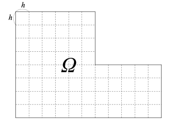
Figure 1: Triangulation $\mathcal{T}_{h}$ of $\overline{\Omega}$ into uniform squares

When we assign a value $c_{m}$ for the midpoint $m$ of each edge in $\mathcal{T}_{h}$, there exists $v_{h}\in{\mathcal{NC}}^{h}(\Omega)$ such that $v_{h}(m)=c_{m}$ at all midpoints $m$ of edges in $\mathcal{T}_{h}$ if and only if

$$c_{m_{1}}+c_{m_{3}}=c_{m_{2}}+c_{m_{4}},$$ (1)

whenever $m_{1},\cdots,m_{4}$ are of clockwisely numbered edges of a square $Q\in\mathcal{T}_{h}.$

For each vertex $\mathbf{V}$ in $\mathcal{T}_{h}$, define a function $\psi^{\mathbf{V}}\in{\mathcal{NC}}^{h}(\Omega)$ by its values at all midpoints $m$ of edges in $\mathcal{T}_{h}$ such that

$$\psi^{\mathbf{V}}(m)=\left\{\begin{array}[]{cl}1,&\mbox{ if }m\mbox{ belongs to an edge which meets }\mathbf{V},\\ 0,&\mbox{ otherwise. }\end{array}\right.$$ (2)

Note $\psi^{\mathbf{V}}\in{\mathcal{NC}}^{h}(\Omega)$ is well defined since its values at the midpoints satisfy the condition (1). Then, we have a basis for ${\mathcal{NC}}^{h}_{0}(\Omega)$ as

$${\mathcal{NC}}^{h}_{0}(\Omega)=\mbox{Span}\{\psi^{\mathbf{V}}\in{\mathcal{NC}}^{h}_{0}(\Omega)\ :\ \mathbf{V}\mbox{ is an interior vertex in }\mathcal{T}_{h}\}.$$ (3)

Hence, the dimension of ${\mathcal{NC}}^{h}_{0}(\Omega)$ is the number of interior vertices in $\mathcal{T}_{h}$ [15, Theorem 2.5].

Define an interpolation $\pi_{h}:H^{1}_{0}(\Omega)\cap C(\Omega)\rightarrow{\mathcal{NC}}^{h}_{0}(\Omega)$ as

$$\pi_{h}v=\sum_{\mathbf{V}}\frac{v(\mathbf{V})}{2}\psi^{\mathbf{V}},\quad\forall v\in H^{1}_{0}(\Omega)\cap C(\Omega),$$ (4)

where the summation runs over all interior vertices $\mathbf{V}$ in $\mathcal{T}_{h}$. We note $\pi_{h}v$ satisfies

$$\pi_{h}v\Big{(}\frac{\mathbf{V}_{1}+\mathbf{V}_{2}}{2}\Big{)}\ =\ \frac{v(\mathbf{V}_{1})+v(\mathbf{V}_{2})}{2}\quad\mbox{ for all adjacent vertices }\mathbf{V}_{1},\mathbf{V}_{2}\mbox{ in }\mathcal{T}_{h}.$$ (5)

Then, the interpolation error is estimated by

$$\|v-\pi_{h}v\|_{L^{2}(\Omega)}+h|v-\pi_{h}v|_{1,h}\ \leq\ C_{\Omega}\,h^{2}|v|_{H^{2}(\Omega)},\quad\forall v\in H^{1}_{0}(\Omega)\cap H^{2}(\Omega),$$

where $|\Box|_{1,h}$ denotes the mesh-dependent discrete $H^{1}$-seminorm such that

$$|\Box|_{1,h}=\left[\sum_{Q\in\mathcal{T}_{h}}\int_{Q}|\nabla\Box|^{2}\,dxdy\right]^{1/2}.$$ (6)

Let $\mathcal{Q}_{1,h}(\Omega)$ be the conforming piecewise bilinear space over $\mathcal{T}_{h}$ as

$$\mathcal{Q}_{1,h}(\Omega)=\{w_{h}\in H_{0}^{1}(\Omega)\cap C(\Omega)\ :\ w_{h}|_{Q}\in\,<1,x,y,xy>\mbox{ for all squares }Q\in\mathcal{T}_{h}\},$$

with an assumption that $\partial\Omega$ consists of segments parallel to $x,y$-axes. Two lowest order finite element spaces $\mathcal{Q}_{1,h}(\Omega)$ and ${\mathcal{NC}}^{h}_{0}(\Omega)$ are isomorphic as in the following lemma.

Lemma 2.1.

Let $\pi_{h}:\mathcal{Q}_{1,h}(\Omega)\rightarrow{\mathcal{NC}}^{h}_{0}(\Omega)$ be the operator as in (4). Then $\pi_{h}$ is a bijection.

Proof.

Let $\pi_{h}v\in{\mathcal{NC}}^{h}_{0}(\Omega)$ vanish at all midpoints of edges in $\mathcal{T}_{h}$ for some $v\in\mathcal{Q}_{1,h}(\Omega)$. Then, $v$ vanishes on each interior edges $E$ in $\mathcal{T}_{h}$ which meets $\partial\Omega$, since $v$ is linear on $E$ and vanishes at the two endpoints of $E$ by (5).

By a sweeping out argument, we conclude that $v$ vanishes on all edges in $\mathcal{T}_{h}$. This means that $\pi_{h}$ is a bijection since the dimensions of $\mathcal{Q}_{1,h}(\Omega)$ and ${\mathcal{NC}}^{h}_{0}(\Omega)$ are same as the number of interior vertices in $\mathcal{T}_{h}$. ∎

For a vector valued function $\mathbf{v}=(v_{1},v_{2})$, the component-wise interpolation and discrete $H^{1}$-seminorm from (4) and (6) will be used as

$$\Pi_{h}\mathbf{v}=(\pi_{h}v_{1},\pi_{h}v_{2}),\quad|\mathbf{v}|_{1,h}=\Big{(}|v_{1}|_{1,h}^{2}+|v_{2}|_{1,h}^{2}\Big{)}^{1/2}.$$

Let $\mathrm{div}_{h}\hskip 1.42262pt,\mathrm{curl}_{h}\hskip 1.42262pt$ be the mesh-dependent discrete divergence and curl as

$$(\mathrm{div}_{h}\hskip 1.42262pt\mathbf{v})\big{|}_{Q}=\mathrm{div}\hskip 1.42262pt(\mathbf{v}|_{Q}),\quad(\mathrm{curl}_{h}\hskip 1.42262pt\mathbf{v})\big{|}_{Q}=\mathrm{curl}\hskip 1.42262pt(\mathbf{v}|_{Q}),\quad\forall Q\in\mathcal{T}_{h}.$$

It is well known there is a constant $C_{\Omega}$ such that [9]

$$|\mathbf{v}|_{[H^{1}(\Omega)]^{2}}\leq C_{\Omega}(\|\mathrm{div}\hskip 1.42262pt\mathbf{v}\|_{L^{2}(\Omega)}+\|\mathrm{curl}\hskip 1.42262pt\mathbf{v}\|_{L^{2}(\Omega)}),\quad\forall\mathbf{v}\in[H^{1}_{0}(\Omega)]^{2}.$$ (7)

We have a similar result to (7) for $[{\mathcal{NC}}^{h}_{0}(\Omega)]^{2}$ in the following lemma.

Lemma 2.2.

For all $\mathbf{v}_{h}\in[{\mathcal{NC}}^{h}_{0}(\Omega)]^{2}$, we have

$$|\mathbf{v}_{h}|_{1,h}^{2}=\|\mathrm{div}_{h}\hskip 1.42262pt\mathbf{v}_{h}\|_{L^{2}(\Omega)}^{2}+\|\mathrm{curl}_{h}\hskip 1.42262pt\mathbf{v}_{h}\|_{L^{2}(\Omega)}^{2}.$$

Proof.

For each $\mathbf{w}_{h}=(w_{1},w_{2})\in[\mathcal{Q}_{1,h}(\Omega)]^{2}$, we have, by integration by parts,

$$\begin{array}[]{ccl}\displaystyle\int_{\Omega}w_{1x}w_{2y}\ dxdy&=&\displaystyle\sum_{Q\in\mathcal{T}_{h}}\int_{Q}w_{1x}w_{2y}\ dxdy\\ &=&\displaystyle\sum_{Q\in\mathcal{T}_{h}}\int_{\partial Q}w_{1x}w_{2}\nu_{y}\ ds-\int_{Q}w_{1xy}w_{2}\ dxdy=-\displaystyle\sum_{Q\in\mathcal{T}_{h}}\int_{Q}w_{1xy}w_{2}\ dxdy,\end{array}$$

since $\nu_{y}$ is nonzero only at the horizontal edges of $\partial Q$ and $w_{1x},w_{2}$ are continuous there. The same argument is repeated to get

$$\begin{array}[]{ccl}\displaystyle\int_{\Omega}w_{1y}w_{2x}\ dxdy&=&\displaystyle\sum_{Q\in\mathcal{T}_{h}}\int_{\partial Q}w_{1y}w_{2}\nu_{x}\ ds-\int_{Q}w_{1yx}w_{2}\ dxdy\\ &=&-\displaystyle\sum_{Q\in\mathcal{T}_{h}}\int_{Q}w_{1yx}w_{2}\ dxdy=\int_{\Omega}w_{1x}w_{2y}\ dxdy.\end{array}$$ (8)

Then, from (8), we can establish

$$\begin{array}[]{lll}\vspace{2mm}|\mathbf{w}_{h}|_{[H^{1}(\Omega)]^{2}}^{2}&=&(w_{1x},w_{1x})+(w_{1y},w_{1y})+(w_{2x},w_{2x})+(w_{2y},w_{2y})\\ \vspace{2mm}&=&(w_{1x}+w_{2y},w_{1x}+w_{2y})+(w_{2x}-w_{1y},w_{2x}-w_{1y})\\ &=&\|\mathrm{div}\hskip 1.42262pt\mathbf{w}_{h}\|_{L^{2}(\Omega)}^{2}+\|\mathrm{curl}\hskip 1.42262pt\mathbf{w}_{h}\|_{L^{2}(\Omega)}^{2}.\end{array}$$ (9)

Now, if $\mathbf{v}_{h}=(v_{1},v_{2})\in[{\mathcal{NC}}^{h}_{0}(\Omega)]^{2}$, there exists $\mathbf{w}_{h}=(w_{1},w_{2})\in[\mathcal{Q}_{1,h}(\Omega)]^{2}$ by Lemma 2.1 such that

$$v_{i}=\pi_{h}w_{i},\quad i=1,2.$$

Given square $Q\in\mathcal{T}_{h}$, assume that

$$w_{i}(x,y)=\alpha_{i}+\beta_{i}\hat{x}+\gamma_{i}\hat{y}+\delta_{i}\hat{x}\hat{y},\quad i=1,2,$$ (10)

where $\hat{x}=x-c_{1},\ \hat{y}=y-c_{2}$ for the center point $(c_{1},c_{2})$ of $Q$. Note

$$\int_{Q}\hat{x}\ dxdy=\int_{Q}\hat{y}\ dxdy=\int_{Q}\hat{x}\hat{y}\ dxdy=0.$$ (11)

By (5), $\pi_{h}\hat{x}\hat{y}$ vanishes at all midpoints of edges in $\mathcal{T}_{h}$ since the values of $\hat{x}\hat{y}$ differ only by their signs at every two endpoints of an edge of $Q$. It means $v_{i}$ is the linear part of $w_{i}$ so that

$$v_{i}(x,y)=\pi_{h}w_{i}(x,y)=\alpha_{i}+\beta_{i}\hat{x}+\gamma_{i}\hat{y},\quad\ i=1,2.$$ (12)

From (10), (11), (12), we expand that

$$\begin{array}[]{l}\vspace{1mm}|\mathbf{w}_{h}|_{[H^{1}(Q)]^{2}}^{2}-\|\mathrm{div}\hskip 1.42262pt\mathbf{w}_{h}\|_{L^{2}(Q)}^{2}-\|\mathrm{curl}\hskip 1.42262pt\mathbf{w}_{h}\|_{L^{2}(Q)}^{2}\\ \qquad\qquad=\displaystyle\int_{Q}(\beta_{1}+\delta_{1}\hat{y})^{2}+(\gamma_{1}+\delta_{1}\hat{x})^{2}+(\beta_{2}+\delta_{2}\hat{y})^{2}+(\gamma_{2}+\delta_{2}\hat{x})^{2}\ dxdy\\ \qquad\qquad\qquad\displaystyle-\int_{Q}(\beta_{1}+\delta_{1}\hat{y}+\gamma_{2}+\delta_{2}\hat{x})^{2}+(\beta_{2}+\delta_{2}\hat{y}-\gamma_{1}-\delta_{1}\hat{x})^{2}\ dxdy\\ \vspace{1mm}\qquad\qquad=\displaystyle\int_{Q}\beta_{1}^{2}+\gamma_{1}^{2}+\beta_{2}^{2}+\gamma_{2}^{2}-(\beta_{1}+\gamma_{2})^{2}-(\beta_{2}-\gamma_{1})^{2}\ dxdy\\ \qquad\qquad=|\mathbf{v}_{h}|_{[H^{1}(Q)]^{2}}^{2}-\|\mathrm{div}\hskip 1.42262pt\mathbf{v}_{h}\|_{L^{2}(Q)}^{2}-\|\mathrm{curl}\hskip 1.42262pt\mathbf{v}_{h}\|_{L^{2}(Q)}^{2}.\end{array}$$

It completes the proof, since $\mathbf{w}_{h}$ satisfies (9). ∎

3 $P_{1}$- nonconforming divergence-free space

Let $V_{h}$ be a locally divergence-free subspace of $[{\mathcal{NC}}^{h}_{0}(\Omega)]^{2}$ as

$$V_{h}=\{\mathbf{v}_{h}\in[{\mathcal{NC}}^{h}_{0}(\Omega)]^{2}\ :\ \mathrm{div}_{h}\hskip 1.42262pt\mathbf{v}_{h}=0\}.$$ (13)

Throughout the remaining of the paper, in order to exclude a pathological triangulation $\mathcal{T}_{h}$ such as a ladder or a union of two rectangles whose intersection is merely one square or edge in $\mathcal{T}_{h}$, we assume that

Assumption 3.1.

No square has 4 boundary vertices. No interior edge meets 2 boundary vertices. If a square has only two boundary vertices, they are the two endpoints of one edge.

Let $\mathcal{P}_{0,h}(\Omega)$ be a space of piecewise constant functions as

$$\mathcal{P}_{0,h}(\Omega)=\{q_{h}\in L^{2}(\Omega)\ :\ q_{h}|_{Q}=<1>\mbox{ for all }Q\in\mathcal{T}_{h}\}.$$

The value of a function $q_{h}\in\mathcal{P}_{0,h}(\Omega)$ at a square $Q\in\mathcal{T}_{h}$ will be abbreviated to $q_{h}(Q)$.

For an interior vertex $\mathbf{V}$, let $Q_{1},Q_{2},Q_{3},Q_{4}$ be the squares in $\mathcal{T}_{h}$ which meet $\mathbf{V}$, counterclockwisely numbered from the square whose left bottom vertex is $\mathbf{V}$ as in Figure 2-(a). Using the scalar basis function $\psi^{\mathbf{V}}\in{\mathcal{NC}}^{h}_{0}(\Omega)$ in (2), for a vector value $(a,b)$, define a function $\psi^{\mathbf{V}}[a,b]\in[{\mathcal{NC}}^{h}_{0}(\Omega)]^{2}$ by its values at all midpoints $m$ of edges in $\mathcal{T}_{h}$ such that

$$\psi^{\mathbf{V}}[a,b](m)=\left\{\begin{array}[]{cl}(a,b),&\mbox{ if }m\mbox{ belongs to an edge which meets }\mathbf{V},\\ (0,0),&\mbox{ otherwise. }\end{array}\right.$$

We can easily check that $\mathrm{div}_{h}\hskip 1.42262pt\psi^{\mathbf{V}}[a,b],\ \mathrm{curl}_{h}\hskip 1.42262pt\psi^{\mathbf{V}}[a,b]\in\mathcal{P}_{0,h}(\Omega)$ have nontrivial values at only 4 squares in $\mathcal{T}_{h}$, given as in Figure 2-(b), (c),

$$\mathrm{div}_{h}\hskip 1.42262pt\psi^{\mathbf{V}}[a,b](Q_{j})=\left\{\begin{array}[]{rl}-(a+b)/h&\mbox{ if }j=1,\\ (a-b)/h&\mbox{ if }j=2,\\ (a+b)/h&\mbox{ if }j=3,\\ (b-a)/h&\mbox{ if }j=4,\end{array}\right.$$ (14)

$$\mathrm{curl}_{h}\hskip 1.42262pt\psi^{\mathbf{V}}[a,b](Q_{j})=\left\{\begin{array}[]{rl}(a-b)/h&\mbox{ if }j=1,\\ (a+b)/h&\mbox{ if }j=2,\\ (b-a)/h&\mbox{ if }j=3,\\ -(a+b)/h&\mbox{ if }j=4.\end{array}\right.$$ (15)

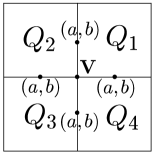
(a) $\psi^{\mathbf{V}}[a,b]$

(b) $\mathrm{div}_{h}\hskip 1.42262pt\psi^{\mathbf{V}}[a,b]$

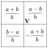
(c) $\mathrm{curl}_{h}\hskip 1.42262pt\psi^{\mathbf{V}}[a,b]$

Figure 2: $\psi^{\mathbf{V}}[a,b]\in[{\mathcal{NC}}^{h}_{0}(\Omega)]^{2}$ and its divergence and curl

3.1 Dimension of $V_{h}$

We call a square $Q\in\mathcal{T}_{h}$ an interior square if it has 4 interior vertices, otherwise, a boundary square. Let $\mathcal{I}_{h}$ be a set of all interior squares in $\mathcal{T}_{h}$ and denote by $\#\mathcal{I}_{h}$ the number of its elements. In the following lemma, $\#\mathcal{I}_{h}$ relates with other numbers depending on $\mathcal{T}_{h}$.

Lemma 3.1.

Let $\mathcal{N}(\mathbf{V}^{i}),\ \mathcal{N}(Q)$ be the numbers of all interior vertices and all squares in $\mathcal{T}_{h}$, respectively. Then,

$$\#\mathcal{I}_{h}\ =\ 2\ \mathcal{N}(\mathbf{V}^{i})-\mathcal{N}(Q)+2.$$ (16)

Proof.

Let $\mathcal{N}(E^{i})$ be the number of all interior edges in $\mathcal{T}_{h}$. Note the number of all boundary vertices, denoted by $\mathcal{N}(\mathbf{V}^{b})$, is same as that of all boundary edges, denoted by $\mathcal{N}(E^{b})$.

Every squares in $\mathcal{T}_{h}$ has 4 edges. When we count them all to make $4\mathcal{N}(Q)$, each interior edges is done twice whereas each boundary edge is done once. That is,

$$4\mathcal{N}(Q)=2\mathcal{N}(E^{i})+\mathcal{N}(E^{b}).$$ (17)

Let $k_{j}$ be the number of all vertices that meet only $j$ squares in $\mathcal{T}_{h}$ for $j=1,2,3,4$. Then, $k_{4}=\mathcal{N}(\mathbf{V}^{i})$ and $k_{2}$ is the number of boundary vertices that are not corners, while $k_{1},k_{3}$ designate those of corners of respective inner angles $90^{\circ},270^{\circ}$.

While we count every 4 vertices of a square in $\mathcal{T}_{h}$ to make $4\mathcal{N}(Q)$, each vertex $\mathbf{V}$ is done repeatedly by its number of squares which meet $\mathbf{V}$. Thus we have,

$$4\mathcal{N}(Q)=k_{1}+2k_{2}+3k_{3}+4k_{4}.$$ (18)

From (17) subtracted by (18),

$$2\mathcal{N}(E^{i})-\mathcal{N}(\mathbf{V}^{b})-4\mathcal{N}(\mathbf{V}^{i})+k_{1}-k_{3}=0,$$ (19)

since $k_{1}+k_{2}+k_{3}=\mathcal{N}(\mathbf{V}^{b})=\mathcal{N}(E^{b})$.

If we paint one boundary square for every one boundary edge, each boundary square that meets a corner of angle $90^{\circ}$ is done twice by Assumption 3.1, while each corner of angle $270^{\circ}$ remains one boundary square unpainted. It means that

$$\mathcal{N}(Q)-\#\mathcal{I}_{h}=\mathcal{N}(E^{b})-k_{1}+k_{3}.$$ (20)

From (20) added by (19), we obtain (16) through the following Euler formula for simply connected domain:

$$\mathcal{N}(Q)-\mathcal{N}(E^{i})+\mathcal{N}(\mathbf{V}^{i})=1.$$

∎

The two-color theorem guarantees that the squares in $\mathcal{T}_{h}$ can be colored in two colors, if each interior vertex meets with even number of edges [19, Ch. 15]. Thus, the squares in $\mathcal{T}_{h}$ are grouped into $\mathcal{R}_{h}$ of the red squares and $\mathcal{K}_{h}$ of the black ones so that squares sharing at least one edge have different colors, as a checkerboard in Figure 3.

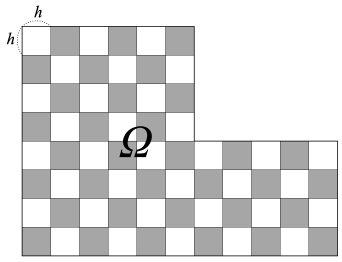
Figure 3: Red and black checkerboard in $\mathcal{T}_{h}$

In the following lemma, if two squares have same color, they are connected by a path which passes only squares of that color and does not meet any boundary vertices. Let

$$\mathcal{R}^{\circ}=\Big{(}\displaystyle\bigcup_{Q\in\mathcal{R}_{h}}\overline{Q}\Big{)}\setminus\partial\Omega,\quad\mathcal{K}^{\circ}=\Big{(}\displaystyle\bigcup_{Q\in\mathcal{K}_{h}}\overline{Q}\Big{)}\setminus\partial\Omega.$$

Lemma 3.2.

$\mathcal{R}^{\circ}$ is path-connected and so is $\mathcal{K}^{\circ}$.

Proof.

It is enough to prove for $\mathcal{R}^{\circ}$. If $\mathbf{x},\mathbf{y}\in\mathcal{R}^{\circ}$, there is a path $\mathscr{P}$ in $\Omega$ joining $\mathbf{x},\mathbf{y}$, since the open set $\Omega$ is connected. We can repair $\mathscr{P}$ into a path in $\mathcal{R}^{\circ}$ in the following way.

Let $\mathbf{c}_{1},\mathbf{c}_{2}$ be two points in the path $\mathscr{P}$ which are on the boundary of a black square $Q_{K}$ and the part of $\mathscr{P}$ between them, named $\mathscr{P}_{12}$, belong to the interior of $Q_{K}$. Denote by $E_{1},E_{2}$, the edges of $Q_{K}$ on which $\mathbf{c}_{1},\mathbf{c}_{2}$ are, respectively. The following 3 cases are possible for $E_{1},E_{2}$.

Case I. If $E_{1}\ =\ E_{2}$, we can easily repair $\mathscr{P}_{12}$ into the segment in $\mathcal{R}^{\circ}$ between $\mathbf{c}_{1},\mathbf{c}_{2}$.

Case II. Let $E_{1},E_{2}$ meet at a vertex $\mathbf{V}$ of $Q_{K}$. If $\mathbf{V}$ is an interior vertex, $\mathscr{P}_{12}$ can be repaired into the 2 segments via $\mathbf{V}$ in $\mathcal{R}^{\circ}$ as in Figure 4-(a). When $\mathbf{V}$ is a boundary vertex, by Assumption 3.1, the other three vertices of $Q_{K}$ are all interior vertices, since $\mathbf{c}_{1},\mathbf{c}_{2}$ belong to $\Omega$. Thus, $\mathscr{P}_{12}$ can be done into the 4 segments in $\mathcal{R}^{\circ}$ which do not pass $\mathbf{V}$ as in Figure 4-(b).

Case III. If $E_{1},E_{2}$ are parallel, by Assumption 3.1, there are endpoints $\mathbf{V}_{1},\mathbf{V}_{2}$ of $E_{1},E_{2}$, respectively, which are interior vertices such that the segment between them is an edge of $Q_{K}$. Thus, $\mathscr{P}_{12}$ can be done into the 3 segments via $\mathbf{V}_{1},\mathbf{V}_{2}$ in $\mathcal{R}^{\circ}$ as in Figure 4-(c).

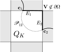
(a) $\overline{E_{1}}\cap\overline{E_{2}}$ is a vertex in $\Omega$

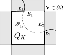
(b) $\overline{E_{1}}\cap\overline{E_{2}}$ is a vertex on $\partial\Omega$

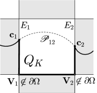
(c) $\overline{E_{1}}\cap\overline{E_{2}}=\emptyset$

Figure 4: The path $\mathscr{P}_{12}$ in $Q_{K}$ (dashed line) is repaired into a path in $\mathcal{R}^{\circ}$ (bold line)

∎

Let $\mathcal{P}^{\prime}_{0,h}(\Omega)$ be a subspace of $\mathcal{P}_{0,h}(\Omega)$ of piecewise constant functions such that

$$\mathcal{P}^{\prime}_{0,h}(\Omega)\ =\ \{q_{h}\in\mathcal{P}_{0,h}(\Omega)\ :\ \int_{\mathcal{R}^{\circ}}q_{h}\ d\sigma=\int_{\mathcal{K}^{\circ}}q_{h}\ d\sigma=0\}.$$

We note $V_{h}$ is the kernel of the operator $\mathrm{div}_{h}\hskip 1.42262pt:[{\mathcal{NC}}^{h}_{0}(\Omega)]^{2}\longrightarrow\mathcal{P}_{0,h}(\Omega)$. The range of $\mathrm{div}_{h}$ is exactly $\mathcal{P}^{\prime}_{0,h}(\Omega)$ in the following lemma.

Lemma 3.3.

$$\mathrm{div}_{h}\hskip 1.42262pt\big{(}[{\mathcal{NC}}^{h}_{0}(\Omega)]^{2}\big{)}=\mathcal{P}^{\prime}_{0,h}(\Omega).$$

Proof.

From (3), $[{\mathcal{NC}}^{h}_{0}(\Omega)]^{2}$ is spanned by $\psi^{\mathbf{V}}[1,0],\psi^{\mathbf{V}}[0,1]$ for all interior vertices $\mathbf{V}$ in $\mathcal{T}_{h}$. By (14), we have

$$\mathrm{div}_{h}\hskip 1.42262pt\psi^{\mathbf{V}}[1,0],\ \mathrm{div}_{h}\hskip 1.42262pt\psi^{\mathbf{V}}[0,1]\in\mathcal{P}^{\prime}_{0,h}(\Omega).$$

It means that

$$\mathrm{div}_{h}\hskip 1.42262pt\big{(}[{\mathcal{NC}}^{h}_{0}(\Omega)]^{2}\big{)}\subset\mathcal{P}^{\prime}_{0,h}(\Omega).$$ (21)

If two red squares $Q_{a},Q_{b}$ meet at an interior vertex $\mathbf{V}$, by (14), there is a function $\mathbf{w}\in[{\mathcal{NC}}^{h}_{0}(\Omega)]^{2}$ which is one of $(h/2)\psi^{\mathbf{V}}[\pm 1,\pm 1]$ such that

$$\mathrm{div}_{h}\hskip 1.42262pt\mathbf{w}(Q_{a})=1,\quad\mathrm{div}_{h}\hskip 1.42262pt\mathbf{w}(Q_{b})=-1,\quad\mathrm{div}_{h}\hskip 1.42262pt\mathbf{w}(Q)=0\mbox{ for all other }Q\in\mathcal{T}_{h}.$$ (22)

Let’s fix one red square $Q_{R}$ in $\mathcal{R}_{h}$. If $Q$ is a red square in $\mathcal{R}_{h}$ different to $Q_{R}$, by Lemma 3.2, there is a path $\mathscr{P}$ in $\mathcal{R}^{\circ}$ joining two center points of $Q$ and $Q_{R}$. Let $\mathscr{P}$ pass through a sequence of $N$ red squares $\{Q_{i}\}_{i=1}^{N}$ in order such that

$$Q_{1}=Q_{R},\quad Q_{N}=Q,\quad{Q}_{i}\neq{Q}_{i+1}\mbox{ for }i=1,2,\cdots,N-1.$$

For each $i=1,2,\cdots,N-1$, $\overline{Q}_{i}\cap\overline{Q}_{i+1}$ is an interior vertex, since $\mathscr{P}$ should pass there and it dose not meet $\partial\Omega$. Thus, as in (22), there is a function $\mathbf{f}_{i}\in[{\mathcal{NC}}^{h}_{0}(\Omega)]^{2}$ such that

$$\mathrm{div}_{h}\hskip 1.42262pt\mathbf{w}_{i}(Q_{i})=1,\quad\mathrm{div}_{h}\hskip 1.42262pt\mathbf{w}_{i}(Q_{i+1})=-1,\quad\mathrm{div}_{h}\hskip 1.42262pt\mathbf{w}_{i}(Q)=0\mbox{ if }Q\neq Q_{i},Q_{i+1}.$$

Then, setting $\mathbf{w}_{h}=\sum_{i=1}^{N-1}\mathbf{w}_{i}\in[{\mathcal{NC}}^{h}_{0}(\Omega)]^{2}$, we have

$$\mathrm{div}_{h}\hskip 1.42262pt\mathbf{w}_{h}(Q_{1})=1,\quad\mathrm{div}_{h}\hskip 1.42262pt\mathbf{w}_{h}(Q_{N})=-1,\quad\mathrm{div}_{h}\hskip 1.42262pt\mathbf{w}_{h}(Q)=0\mbox{ if }Q\neq Q_{1},Q_{N}.$$ (23)

Since these arguments can be repeated for the black squares in $\mathcal{K}_{h}$, (23) means the range of $\mathrm{div}_{h}\hskip 1.42262pt$ has at least $\mathcal{N}(Q)-2$ linear independent piecewise constant functions. It is combined with (21) to complete the proof. ∎

Now, we reach at the theorem for the dimension of $V_{h}$.

Theorem 3.4.

The dimension of $V_{h}$ is the number of interior squares in $\mathcal{T}_{h}$.

Proof.

Since $V_{h}$ is the kernel of $\mathrm{div}_{h}\hskip 1.42262pt$, by (3) and Lemma 3.1 and 3.3, we have

$$\dim(V_{h}) = \dim([{\mathcal{NC}}^{h}_{0}(\Omega)]^{2})-\dim\Big{(}\mathrm{div}_{h}\hskip 1.42262pt\big{(}[{\mathcal{NC}}^{h}_{0}(\Omega)]^{2}\big{)}\Big{)}$$

$$= 2\mathcal{N}(\mathbf{V}^{i})-(\mathcal{N}(Q)-2)=\#\mathcal{I}_{h}.$$

∎

3.2 Basis for $V_{h}$

For each square $Q$ in $\mathcal{T}_{h}$, denote by $\mathbf{V}^{rt}(Q),\mathbf{V}^{lt}(Q),\mathbf{V}^{lb}(Q),\mathbf{V}^{rb}(Q)$, respective vertices of $Q$ in the right top, left top, left bottom, right bottom corners of $Q$ as depicted in Figure 5. Let $Q^{rt},Q^{lt},Q^{lb},Q^{rb}$ be squares in $\mathcal{T}_{h}$ whose closures intersect with $\overline{Q}$ at only $\mathbf{V}^{rt}(Q)$, $\mathbf{V}^{lt}(Q)$, $\mathbf{V}^{lb}(Q)$, $\mathbf{V}^{rb}(Q)$, respectively. If $Q\in\mathcal{T}_{h}$ is a boundary square, some of them are empty.

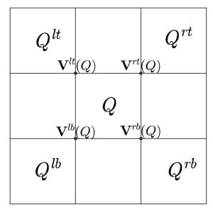
Figure 5: Name convention

For each interior square $Q\in\mathcal{I}_{h}$, define a locally divergence-free function $\mathbf{\Psi}_{h}^{Q}\in V_{h}$ by

$$\mathbf{\Psi}_{h}^{Q}=\psi^{\mathbf{V}^{rt}(Q)}[\frac{1}{2},-\frac{1}{2}]+\psi^{\mathbf{V}^{lt}(Q)}[\frac{1}{2},\frac{1}{2}]+\psi^{\mathbf{V}^{lb}(Q)}[-\frac{1}{2},\frac{1}{2}]+\psi^{\mathbf{V}^{rb}(Q)}[-\frac{1}{2},-\frac{1}{2}].$$

The nontrivial values of $\mathbf{\Psi}_{h}^{Q}$ at the midpoints of edges in $\mathcal{T}_{h}$ are depicted in Figure 6-(a). With (14), (15), we can easily check that $\mathrm{div}_{h}\hskip 1.42262pt\mathbf{\Psi}_{h}^{Q}$ vanishes in all squares and

$$\mathrm{curl}_{h}\hskip 1.42262pt\mathbf{\Psi}_{h}^{Q}=\left\{\begin{array}[]{cl}-4/h&\mbox{ in }Q,\\ 1/h&\mbox{ in }Q^{rt},Q^{lt},Q^{lb},Q^{rb},\\ 0&\mbox{ in other squares,}\end{array}\right.$$ (24)

as in Figure 6-(b).

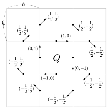
(a) Nontrivial values of $\mathbf{\Psi}_{h}^{Q}$ at midpoints

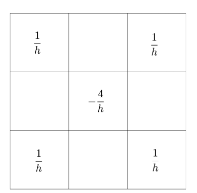
(b) Nontrivial values of $\mathrm{curl}_{h}\hskip 1.42262pt\mathbf{\Psi}_{h}^{Q}$

Figure 6: Divergence-free $\mathbf{\Psi}_{h}^{Q}\in V_{h}$ centered at an interior square $Q$

Then, we are able to specify a basis for $V_{h}$ in the following theorem.

Theorem 3.5.

The set $\mathcal{B}=\{\mathbf{\Psi}_{h}^{Q}\ :\ Q\mbox{ is an interior square in }\mathcal{T}_{h}\}$ is a basis for $V_{h}$,

Proof.

By Theorem 3.4, the linear independency of $\mathcal{B}$ completes the proof. If a linear combination of functions in $\mathcal{B}$ vanish, does its discrete curl, too. Thus, it is sufficient to prove that the following set $\mathscr{F}_{h}$ is linearly independent,

$$\mathscr{F}_{h}=\{\mathrm{curl}_{h}\hskip 1.42262pt\mathbf{\Psi}_{h}^{Q}\ :\ Q\mbox{ is an interior square in }\mathcal{T}_{h}\}.$$

For each square $Q\in\mathcal{T}_{h}$, we define a piecewise constant function $\mathbf{f}_{Q}\in\mathcal{P}_{0,h}(\Omega)$ by

$$\mathbf{f}_{Q}=\left\{\begin{array}[]{cl}-4&\mbox{ in }Q,\\ 1&\mbox{ in }Q^{rt},Q^{lt},Q^{lb},Q^{rb},\\ 0&\mbox{ in other squares}.\end{array}\right.$$ (25)

Let $N$ be the number of all red squares in $\mathcal{R}_{h}$ which are numbered as $Q_{1},Q_{2},\cdots,Q_{N}$. Regarding $\mathbf{f}_{Q_{j}}$ as a column vector in $\mathbb{R}^{N}$ for each $j=1,2,\cdots,N$, we have an $N\times N$ matrix $M_{R}$ such that

$$M_{R}=[\mathbf{f}_{Q_{1}},\mathbf{f}_{Q_{2}},\cdots,\mathbf{f}_{Q_{N}}].$$

By the definition $\mathbf{f}_{Q}$ in (25), all columns of $M_{R}$ are diagonally dominant and, if $Q_{j}$ is a boundary square, the $j$-th column is strictly diagonally dominant. Furthermore, by Lemma 3.2, $M_{R}$ is irreducible, since $M_{R}(i,j)$ is nonzero whenever $\overline{Q_{i}},\overline{Q_{j}}$ intersect for $i,j=1,2,\cdots,N$. Thus by Taussky theorem, $M_{R}$ is invertible [11]. Then, since $\mathbf{f}_{Q}$ is $\mathrm{curl}_{h}\hskip 1.42262pt\mathbf{\Psi}_{h}^{Q}$ in (24) multiplied by $h$, the following set is linearly independent,

$$\mathscr{F}_{h}^{R}=\{\mathrm{curl}_{h}\hskip 1.42262pt\mathbf{\Psi}_{h}^{Q}\ :\ Q\mbox{ is an interior red square in }\mathcal{T}_{h}\}.$$

Repeating same arguments for the black squares in $\mathcal{K}_{h}$, we have the following $\mathscr{F}_{h}^{K}$ is also linearly independent,

$$\mathscr{F}_{h}^{K}=\{\mathrm{curl}_{h}\hskip 1.42262pt\mathbf{\Psi}_{h}^{Q}\ :\ Q\mbox{ is an interior black square in }\mathcal{T}_{h}\}.$$

For a red square $Q$ and a black one $Q^{\prime}$, the supports of $\mathrm{curl}_{h}\hskip 1.42262pt\mathbf{\Psi}_{h}^{Q}$ and $\mathrm{curl}_{h}\hskip 1.42262pt\mathbf{\Psi}_{h}^{Q^{\prime}}$ do not intersect. Therefore, we conclude that $\mathscr{F}_{h}=\mathscr{F}_{h}^{R}\cup\mathscr{F}_{h}^{K}$ is linearly independent. ∎

The basis for $V_{h}$ in Theorem 3.5 plays an important role in error analysis of the conforming $\mathcal{Q}_{1,h}(\Omega)-\mathcal{P}_{0,h}(\Omega)$ with the dimension of $V_{h}$ in Theorem 3.4 [16].

4 Application for incompressible Stokes problems

Let $(\mathbf{u},p)\in[H_{0}^{1}(\Omega)]^{2}\times L_{0}^{2}(\Omega)$ be the solution of the variational form of an incompressible Stokes equation:

$$(\nabla\mathbf{u},\nabla\mathbf{v})-(p,\mathrm{div}\hskip 1.42262pt\mathbf{v})+(q,\mathrm{div}\hskip 1.42262pt\mathbf{u})=(\mathbf{f},\mathbf{v}),\quad\forall(\mathbf{v},q)\in[H_{0}^{1}(\Omega)]^{2}\times L_{0}^{2}(\Omega),$$

for a source function $\mathbf{f}\in[L^{2}(\Omega)]^{2}$.

For the finite element solution, let $(\mathbf{u}_{h},p_{h})\in[{\mathcal{NC}}^{h}_{0}(\Omega)]^{2}\times\mathcal{P}^{\prime}_{0,h}(\Omega)$ satisfies that

$$(\nabla\mathbf{u}_{h},\nabla\mathbf{v}_{h})-(p_{h},\mathrm{div}\hskip 1.42262pt\mathbf{v}_{h})+(q_{h},\mathrm{div}\hskip 1.42262pt\mathbf{u}_{h})=(\mathbf{f},\mathbf{v}_{h}),\quad\forall(\mathbf{v}_{h},q_{h})\in[{\mathcal{NC}}^{h}_{0}(\Omega)]^{2}\times\mathcal{P}^{\prime}_{0,h}(\Omega).$$ (26)

If $\mathbf{u}\in[H^{2}(\Omega)]^{2},p\in H^{1}(\Omega)$, the following error estimate holds

$$|\mathbf{u}-\mathbf{u}_{h}|_{1,h}+\|p-p_{h}\|_{0}\leq C_{\Omega}h(|\mathbf{u}|_{2}+|p|_{1}),$$ (27)

since $[{\mathcal{NC}}^{h}_{0}(\Omega)]^{2}\times\mathcal{P}^{\prime}_{0,h}(\Omega)$ satisfies the inf-sup condition [13].

In an alternate way to get $(\mathbf{u}_{h},p_{h})\in[{\mathcal{NC}}^{h}_{0}(\Omega)]^{2}\times\mathcal{P}^{\prime}_{0,h}(\Omega)$ in (26), we can solve an elliptic problem for velocity and apply an explicit method for pressure as in next two subsections.

4.1 Elliptic problem for velocity

The discrete velocity $\mathbf{u}_{h}$ in (26) satisfies that

$$(q_{h},\mathrm{div}\hskip 1.42262pt\mathbf{u}_{h})=0,\quad\mbox{for all }q_{h}\in\mathcal{P}^{\prime}_{0,h}(\Omega).$$

Since there exists $q_{h}\in\mathcal{P}^{\prime}_{0,h}(\Omega)$ such that $q_{h}=\mathrm{div}\hskip 1.42262pt\mathbf{u}_{h}$ from (14), we have

$$\mathbf{u}_{h}\in V_{h},$$

for the locally divergence-free finite element space $V_{h}$ in (13). Thus, to get $\mathbf{u}_{h}$ in (26), we can solve the following elliptic problem for velocity:

$$(\nabla\mathbf{u}_{h},\nabla\mathbf{v}_{h})=(\mathbf{f},\mathbf{v}_{h}),\quad\forall\mathbf{v}_{h}\in V_{h},$$ (28)

which smaller than the problem (26).

We note, since the norm is decomposed in Lemma 2.2, so is the inner product as

$$(\nabla\mathbf{v}_{h},\nabla\mathbf{w}_{h})=(\mathrm{div}_{h}\hskip 1.42262pt\mathbf{v}_{h},\mathrm{div}_{h}\hskip 1.42262pt\mathbf{w}_{h})+(\mathrm{curl}_{h}\hskip 1.42262pt\mathbf{v}_{h},\mathrm{curl}_{h}\hskip 1.42262pt\mathbf{w}_{h}),\quad\forall\mathbf{v}_{h},\mathbf{w}_{h}\in[{\mathcal{NC}}^{h}_{0}(\Omega)]^{2}.$$

The above means

$$(\nabla\mathbf{v}_{h},\nabla\mathbf{w}_{h})=(\mathrm{curl}_{h}\hskip 1.42262pt\mathbf{v}_{h},\mathrm{curl}_{h}\hskip 1.42262pt\mathbf{w}_{h}),\quad\forall\mathbf{v}_{h},\mathbf{w}_{h}\in V_{h}.$$

Thus, the problem (28) is equivalent to

$$(\mathrm{curl}_{h}\hskip 1.42262pt\mathbf{u}_{h},\mathrm{curl}_{h}\hskip 1.42262pt\mathbf{v}_{h})=(\mathbf{f},\mathbf{v}_{h}),\quad\forall\mathbf{v}_{h}\in V_{h}.$$ (29)

Suggested in Theorem 3.5, a basis $\mathcal{B}$ for $V_{h}$ consists of $\mathbf{\Psi}_{h}^{Q}$ for all interior square $Q\in\mathcal{T}_{h}$. For an interior square $Q$, although the support of the basis function $\mathbf{\Psi}_{h}^{Q}$ in $V_{h}$ consists of 9 squares, that of $\mathrm{curl}_{h}\hskip 1.42262pt\mathbf{\Psi}_{h}^{Q}$ is 5 squares as in Figure 6. If we assume $h=1$ for simplicity, as in Figure 7, 8, 9, 10, we have

$$(\nabla\mathbf{\Psi}_{h}^{Q},\nabla\mathbf{\Psi}_{h}^{Q^{\prime}})=\left\{\begin{array}[]{cl}20&\mbox{ if }Q=Q^{\prime},\\ 2&\mbox{ if supports of }\nabla\mathbf{\Psi}_{h}^{Q},\nabla\mathbf{\Psi}_{h}^{Q^{\prime}}\mbox{ meet at 3 squares},\\ -8&\mbox{ if supports of }\nabla\mathbf{\Psi}_{h}^{Q},\nabla\mathbf{\Psi}_{h}^{Q^{\prime}}\mbox{ meet at 4 squares},\\ 1&\mbox{ if supports of }\nabla\mathbf{\Psi}_{h}^{Q},\nabla\mathbf{\Psi}_{h}^{Q^{\prime}}\mbox{ meet at 1 square}.\end{array}\right.$$

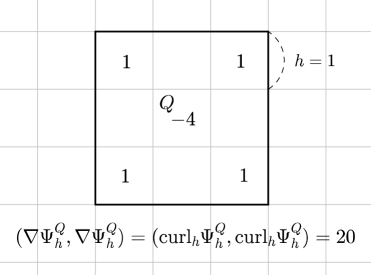
Figure 7: Inner product $(\nabla\mathbf{\Psi}_{h}^{Q},\nabla\mathbf{\Psi}_{h}^{Q})$ when $h=1$

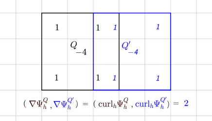
Figure 8: Inner product of $\nabla\mathbf{\Psi}_{h}^{Q},{\color[rgb]{0,0,1}\nabla\mathbf{\Psi}_{h}^{Q^{\prime}}}$ when their supports meet at 3 squares

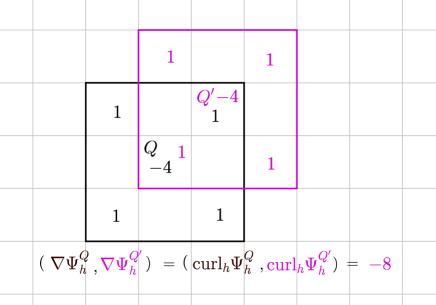
Figure 9: Inner product of $\nabla\mathbf{\Psi}_{h}^{Q},{\color[rgb]{0.55,0.14,1}\nabla\mathbf{\Psi}_{h}^{Q^{\prime}}}$ when their supports meet at 4 squares

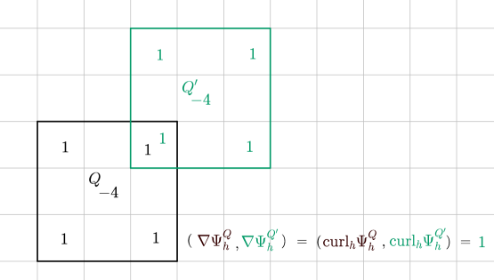
Figure 10: Inner product of $\nabla\mathbf{\Psi}_{h}^{Q},{\color[rgb]{0,0.6015625,0.3984375}\nabla\mathbf{\Psi}_{h}^{Q^{\prime}}}$ when their supports meet at 1 square

Besides, if $Q$ is a red square, the support of $\mathrm{curl}_{h}\hskip 1.42262pt\mathbf{\Psi}_{h}^{Q}$ lies in 5 red squares, and vice versa for a black square. Thus, their supports do not meet each other as in Figure 11. It means the following lemma.

Lemma 4.1.

For each interior red square $Q_{R}$ and black square $Q_{K}$,

$$(\nabla\mathbf{\Psi}_{h}^{Q_{R}},\nabla\mathbf{\Psi}_{h}^{Q_{K}})=0.$$

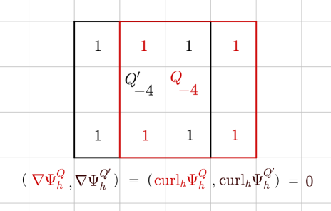
Figure 11: ${\color[rgb]{1,0,0}\mathrm{curl}_{h}\hskip 1.42262pt\mathbf{\Psi}_{h}^{Q}}$ for red square $\color[rgb]{1,0,0}Q$, $\mathrm{curl}_{h}\hskip 1.42262pt\mathbf{\Psi}_{h}^{Q^{\prime}}$ for black square $Q^{\prime}$ : They do not meet.

As a result, when we implement the finite element method to solve (28) with the basis $\mathcal{B}$ for $V_{h}$, the inner products $(\nabla\mathbf{\Psi}_{h}^{Q},\nabla\mathbf{\Psi}_{h}^{Q^{\prime}})$ vanish except at most 13 $Q^{\prime}$ for a fixed interior square $Q\in\mathcal{T}_{h}$, as in Figure 12. Thus the sparsity of the system of linear equations is not as large as expected from the support of $\mathbf{\Psi}_{h}^{Q}$.

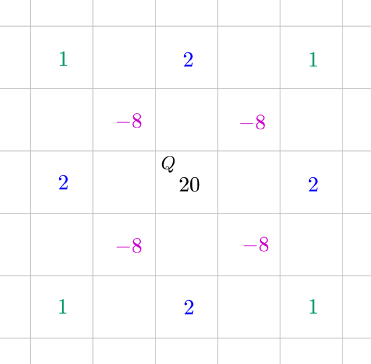
Figure 12: 13 nonzero ($\nabla\mathbf{\Psi}_{h}^{Q},\nabla\mathbf{\Psi}_{h}^{Q^{\prime}})$ for fixed $Q$

Furthermore, by Lemma 4.1, the system of linear equations to solve (28) with the basis $\mathcal{B}$ for $V_{h}$ can be split into two smaller ones with the following $\mathcal{B}_{R},\mathcal{B}_{K}$ for red and black squares, respectively,

$$\begin{array}[]{ccc}\vspace{2mm}\mathcal{B}_{R}&=&\{\mathbf{\Psi}_{h}^{Q}\ :\ Q\mbox{ is an interior red square in }\mathcal{T}_{h}\},\\ \mathcal{B}_{K}&=&\{\mathbf{\Psi}_{h}^{Q}\ :\ Q\mbox{ is an interior black square in }\mathcal{T}_{h}\}.\end{array}$$ (30)

$P_{1}$-nonconforming finite elements extend to a general polygonal domain on triangulations into squares and triangles [1]. Based on the proposed method, we can develop a method to solve velocity first for Stokes problems on those mixed meshes.

4.2 Explicit method for pressure recovery

We will find the discrete pressure $p_{h}\in\mathcal{P}^{\prime}_{0,h}(\Omega)$ in (26) by an explicit method using the a priori obtained discrete velocity $\mathbf{u}_{h}\in V_{h}$ in (26) through the elliptic problem (28).

Let’s consider the problem (P): Find $a_{h}\in\mathcal{P}^{\prime}_{0,h}(\Omega)$ such that

$$(a_{h},\mathrm{div}_{h}\hskip 1.42262pt\mathbf{v}_{h})=(\nabla\mathbf{u}_{h},\nabla\mathbf{v}_{h})-(\mathbf{f},\mathbf{v}_{h}),\quad\forall\mathbf{v}_{h}\in[{\mathcal{NC}}^{h}_{0}(\Omega)]^{2}.$$

By Lemma 3.3, $p_{h}\in\mathcal{P}^{\prime}_{0,h}(\Omega)$ in (26) is the unique solution of the problem (P).

Define two checkerboard functions $\chi_{R},\chi_{K}\in\mathcal{P}_{0,h}(\Omega)$ by

$$\chi_{R}({Q})=\left\{\begin{array}[]{cl}1,&\mbox{ if }Q\mbox{ is a red square,}\\ 0,&\mbox{ if }Q\mbox{ is a black square,}\end{array}\right.\quad\chi_{K}({Q})=\left\{\begin{array}[]{cl}0,&\mbox{ if }Q\mbox{ is a red square,}\\ 1,&\mbox{ if }Q\mbox{ is a black square.}\end{array}\right.$$

We have, for all $\mathbf{v}_{h}\in[{\mathcal{NC}}^{h}_{0}(\Omega)]^{2}$,

$$(\chi_{R},\mathrm{div}_{h}\hskip 1.42262pt\mathbf{v}_{h})=(\chi_{K},\mathrm{div}_{h}\hskip 1.42262pt\mathbf{v}_{h})=(\chi_{R},\chi_{K})=0.$$ (31)

Let’s fix a red square $Q_{R}$, a black one $Q_{K}$ and define $\hat{p_{h}}\in\mathcal{P}_{0,h}(\Omega)$ by

$$\hat{p_{h}}=p_{h}-C_{R}\chi_{R}-C_{k}\chi_{K},$$

for two constants $C_{R}=p_{h}({Q_{R}}),C_{K}=p_{h}({Q_{K}})$. Then, by (31), $\hat{p_{h}}\in\mathcal{P}_{0,h}(\Omega)$ satisfies

$$\begin{array}[]{c}\vspace{2mm}(\hat{p_{h}},\mathrm{div}_{h}\hskip 1.42262pt\mathbf{v}_{h})=(\nabla\mathbf{u}_{h},\nabla\mathbf{v}_{h})-(\mathbf{f},\mathbf{v}_{h}),\quad\forall\mathbf{v}_{h}\in[{\mathcal{NC}}^{h}_{0}(\Omega)]^{2},\\ \hat{p_{h}}({Q_{R}})=\hat{p_{h}}({Q_{K}})=0.\end{array}$$ (32)

We will find $\hat{p_{h}}$ satisfying (32) by an explicit method. If other red square $Q_{R}^{\prime}$ meets with $Q_{R}$ at an interior vertex, there is a function $\mathbf{v}_{h}\in[{\mathcal{NC}}^{h}_{0}(\Omega)]^{2}$ as in (22) such that

$$\mathrm{div}_{h}\hskip 1.42262pt\mathbf{v}_{h}({Q_{R}^{\prime}})=1,\quad\mathrm{div}_{h}\hskip 1.42262pt\mathbf{v}_{h}({Q_{R}})=-1,\quad\mathrm{div}_{h}\hskip 1.42262pt\mathbf{v}_{h}(Q)=0\mbox{ for all other }Q\in\mathcal{T}_{h}.$$ (33)

Then, from (32) and (33), $\hat{p_{h}}$ at $Q_{R}^{\prime}$ is determined by

$$\int_{Q_{R}^{\prime}}\hat{p_{h}}\ d\sigma=\int_{Q_{R}}\hat{p_{h}}\ d\sigma+(\nabla\mathbf{u}_{h},\nabla\mathbf{v}_{h})-(\mathbf{f},\mathbf{v}_{h}).$$

In this manner, we can find $\hat{p_{h}}$ at all red squares by an explicit telescoping methods using such simple $\mathrm{div}_{h}\hskip 1.42262pt\mathbf{v}_{h}$ as in (33), since all red ones are connected through interior vertices as in the proof of Theorem 3.4. Applying the same telescoping methods for the black squares, we get a piecewise constant function $\hat{p_{h}}\in\mathcal{P}_{0,h}(\Omega)$ satisfying (32).

Then, we can obtain the unique solution $p_{h}\in\mathcal{P}^{\prime}_{0,h}(\Omega)$ of the problem (P) so that

$$p_{h}=\hat{p_{h}}-D_{R}\chi_{R}-D_{K}\chi_{K},$$

where $D_{R}$ and $D_{K}$ are constants such that

$$D_{R}=\frac{(\hat{p_{h}},\chi_{R})}{(\chi_{R},\chi_{R})},\quad D_{K}=\frac{(\hat{p_{h}},\chi_{K})}{(\chi_{K},\chi_{K})}.$$

5 Numerical results

We chose the velocity $\mathbf{u}$ and pressure $p$ on $\Omega=[0,1]^{2}$ for numerical tests, as

$$\mathbf{u}=(\phi_{y},-\phi_{x}),\quad p=\sin(4\pi x)e^{\pi y},$$

where $\phi$ is the stream function such that

$$\phi(x,y)=\sin(2\pi x)\sin(3\pi y)(x^{3}-x)(y^{2}-y).$$

The discrete velocity $\mathbf{u}_{h}$ is the sum of two solutions of the problems (29) in $V_{h}$ with two separable bases $\mathcal{B}_{R}$ and $\mathcal{B}_{K}$ in (30) for red and black squares, respectively.

The cardinalities of $\mathcal{B}_{R}$ and $\mathcal{B}_{K}$ are same and much smaller than the dimension of the entire space $[{\mathcal{NC}}^{h}_{0}(\Omega)]^{2}\times\mathcal{P}^{\prime}_{0,h}(\Omega)$ as in Table 1. Each system of linear equations with $\mathcal{B}_{R}$ and $\mathcal{B}_{K}$ was solved by a direct method based on the Cholesky decomposition.

The condition numbers of the elliptic problem (29) in $\|\cdot\|_{\infty}$ norm increase with the order of $O(h^{-4})$ listed in Table 2 as well as those of the saddle point problem (26). The structures of non-zero entries in the concerning matrices are depicted in Figure 13 over $16\times 16$ mesh with the lexicographical basis numbering.

After solving $\mathbf{u}_{h}$, we obtained the discrete pressure $p_{h}$ by the explicit method suggested in subsection 4.2. The numerical results in Table 3 show the optimal order of error decay expected in (27).

mesh	$\dim(\mbox{Span }\mathcal{B}_{R})=\dim(\mbox{Span }\mathcal{B}_{K})$	$\dim\big{(}[{\mathcal{NC}}^{h}_{0}(\Omega)]^{2}\times\mathcal{P}^{\prime}_{0,h}(\Omega)\big{)}$
8 x 8	18	160
16 x 16	98	704
32 x 32	450	2,944
64 x 64	1,922	12,032
128 x 128	7,938	48,640
256 x 256	32,258	195,584
512 x 512	130,050	784,384
1024 x 1024	522,242	3,141,632

Table 1: Dimensions of $\mbox{Span }\mathcal{B}_{R},\mbox{Span }\mathcal{B}_{K}$ and $[{\mathcal{NC}}^{h}_{0}(\Omega)]^{2}\times\mathcal{P}^{\prime}_{0,h}(\Omega)$

mesh	elliptic problem (29)		saddle point problem (26)
	with $\mbox{Span }\mathcal{B}_{R}$		with $[{\mathcal{NC}}^{h}_{0}(\Omega)]^{2}\times\mathcal{P}^{\prime}_{0,h}(\Omega)$
	condition number	order	condition number	order
8 x 8	8.3345E+1		1.4573E+5
16 x 16	1.3284E+3	15.93	2.3375E+6	16.03
32 x 32	2.1235E+4	15.98	3.7251E+7	15.93
64 x 64	3.3968E+5	15.99	5.9424E+8	15.95
128 x 128	5.4346E+6	15.99	9.4913E+9	15.97

Table 2: condition numbers in $\|\cdot\|_{\infty}$ norm

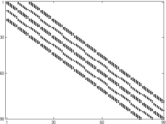
(a) Elliptic problem whose rank is $98$

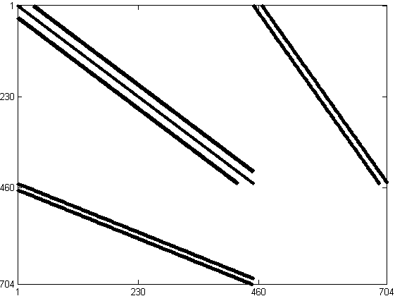
(b) Saddle point problem whose rank is $704$

Figure 13: Structures of non-zero entries in the concerning matrices over $16\times 16$ mesh

mesh	$\|\mathbf{u}-\mathbf{u}_{h}\|_{0}$		$|\mathbf{u}-\mathbf{u}_{h}|_{1,h}$		$\|p-p_{h}\|_{0}$
	value	order	value	order	value	order
8 x 8	5.6091E-2		2.1164E+0		2.9913E+0
16 x 16	1.3451E-2	2.0601	1.0774E+0	0.9740	1.5145E+0	0.9819
32 x 32	3.3342E-3	2.0123	5.4115E-1	0.9935	7.6081E-1	0.9933
64 x 64	8.3187E-4	2.0029	2.7088E-1	0.9984	3.8088E-1	0.9982
128 x 128	2.0786E-4	2.0007	1.3548E-1	0.9996	1.9050E-1	0.9995
256 x 256	5.1959E-5	2.0002	6.7743E-2	0.9999	9.5257E-2	0.9999
512 x 512	1.2990E-5	2.0000	3.3872E-2	1.0000	4.7630E-2	1.0000
1024 x 1024	3.2497E-6	1.9990	1.6936E-2	1.0000	2.3815E-2	1.0000

Table 3: Error table for the divergence-free method