Curves of equiharmonic solutions, and problems at resonance

Abstract

We consider the semilinear Dirichlet problem

$$\Delta u+kg(u)=\mu_{1}\varphi_{1}+\cdots+\mu_{n}\varphi_{n}+e(x)\;\;\mbox{for $x\in\Omega$},\;\;u=0\;\;\mbox{on $\partial\Omega$},$$

where $\varphi_{k}$ is the $k$-th eigenfunction of the Laplacian on $\Omega$ and $e(x)\perp\varphi_{k}$, $k=1,\ldots,n$. Write the solution in the form $u(x)=\Sigma_{i=1}^{n}\xi_{i}\varphi_{i}+U(x)$, with $U\perp\varphi_{k}$, $k=1,\ldots,n$. Starting with $k=0$, when the problem is linear, we continue the solution in $k$ by keeping $\xi=(\xi_{1},\ldots,\xi_{n})$ fixed, but allowing for $\mu=(\mu_{1},\ldots,\mu_{n})$ to vary. Studying the map $\xi\rightarrow\mu$ provides us with the existence and multiplicity results for the above problem. We apply our results to problems at resonance, at both the principal and higher eigenvalues. Our approach is suitable for numerical calculations, which we implement, illustrating our results.

Key words: Curves of equiharmonic solutions, problems at resonance.

AMS subject classification: 35J60.

1 Introduction

We study existence and multiplicity of solutions for a semilinear problem

(1.1) $$\Delta u+kg(u)=f(x)\;\;\mbox{for $x\in\Omega$}\,,$$

$$u=0\;\;\mbox{on $\partial\Omega$}$$

on a smooth bounded domain $\Omega\subset R^{m}$. Here the functions $f(x)\in L^{2}(\Omega)$ and $g(u)\in C^{1}(R)$ are given, $k$ is a parameter. We approach this problem by continuation in $k$. When $k=0$ the problem is linear. It has a unique solution, as can be seen by using Fourier series of the form $u(x)=\Sigma_{j=1}^{\infty}u_{j}\varphi_{j}$, where $\varphi_{j}$ is the $j$-th eigenfunction of the Dirichlet Laplacian on $\Omega$, with $\int_{\Omega}\varphi_{j}^{2}\,dx=1$, and $\lambda_{j}$ is the corresponding eigenvalue. We now continue the solution in $k$, looking for a solution pair $(k,u)$, or $u=u(x,k)$. At a generic point $(k,u)$ the implicit function theorem applies, allowing the continuation in $k$. These are the regular points, where the corresponding linearized problem has only the trivial solution. So until a singular point is encountered, we have a solution curve $u=u(x,k)$. At a singular point practically anything imaginable might happen. At some singular points the M.G. Crandall and P.H. Rabinowitz bifurcation theorem [5] applies, giving us a curve of solutions through a singular point. But even in this favorable situation there is a possibility that solution curve will “turn back” in $k$.

In [10] we have presented a way to continue solutions forward in $k$, which can take us through any singular point. We describe it next. If a solution $u(x)$ is given by its Fourier series $u(x)=\Sigma_{j=1}^{\infty}\xi_{j}\varphi_{j}$, we call $U_{n}=(\xi_{1},\xi_{2},\ldots,\xi_{n})$ the $n$-signature of solution, or just signature for short. We also represent $f(x)$ by its Fourier series, and rewrite the problem (1.1) as

(1.2) $$\Delta u+kg(u)=\mu^{0}_{1}\varphi_{1}+\cdots+\mu^{0}_{n}\varphi_{n}+e(x)\;\;\mbox{for $x\in\Omega$},$$

$$u=0\;\;\mbox{on $\partial\Omega$}$$

with $\mu^{0}_{j}=\int_{\Omega}f\varphi_{j}\,dx$, and $e(x)$ is the projection of $f(x)$ onto the orthogonal complement to $\varphi_{1},\ldots,\varphi_{n}$. Let us now constrain ourselves to hold the signature $U_{n}$ fixed (when continuing in $k$), and in return allow for $\mu_{1},\ldots,\mu_{n}$ to vary. I.e., we are looking for $(u,\mu_{1},\ldots,\mu_{n})$ as a function of $k$, with $U_{n}$ fixed, solving

(1.3) $$\;\;\;\;\;\;\Delta u+kg(u)=\mu_{1}\varphi_{1}+\cdots+\mu_{n}\varphi_{n}+e(x)\;\;\mbox{for $x\in\Omega$},\;\;u=0\;\;\mbox{on $\partial\Omega$}\,,$$

$$\int_{\Omega}u\varphi_{i}\,dx=\xi_{i},\;\;i=1,\dots,n\,.$$

It turned out that we can continue forward in $k$ this way, so long as

(1.4) $$k\max_{u\in R}g^{\prime}(u)<\lambda_{n+1}\,.$$

In the present paper we present a much simplified proof of this result, and generalize it for the case of $(i,n)$ signatures (defined below). Then, we present two new applications.

So suppose the condition (1.4) holds, and we wish to solve the problem (1.2) at some $k=k_{0}$. We travel in $k$, from $k=0$ to $k=k_{0}$, on a curve of fixed signature $U_{n}=(\xi_{1},\xi_{2},\ldots,\xi_{n})$, obtaining a solution $(u,\mu_{1},\ldots,\mu_{n})$ of (1.3). The right hand side of (1.3) has the first $n$ harmonics different (in general) from the ones we want in (1.2). We now vary $U_{n}$. The question is: can we choose $U_{n}$ to obtain the desired $\mu_{1}=\mu^{0}_{1},\ldots,\mu_{n}=\mu^{0}_{n}$, and if so, in how many ways? This corresponds to the existence and multiplicity questions for the original problem (1.1). In [10] we obtained this way a unified approach to the well known results of E.M. Landesman and A.C. Lazer [12], A. Ambrosetti and G. Prodi [2], M. S. Berger and E. Podolak [4], H. Amann and P. Hess [1] and D.G. de Figueiredo and W.-M. Ni [7]. We also provided some new results on “jumping nonlinearities”, and on symmetry breaking.

Our main new application in the present paper is to unbounded perturbations at resonance, which we describe next. For the problem

$$\Delta u+\lambda_{1}u+g(u)=e(x)\;\;\mbox{on $\Omega$},\;\;u=0\;\;\mbox{on $\partial\Omega$}\,,$$

with a bounded $g(u)$, satisfying $ug(u)\geq 0$ for all $u\in R$, and $e(x)\in L^{\infty}(\Omega)$ satisfying $\int_{\Omega}e(x)\varphi_{1}(x)\,dx=0$, D.G. de Figueiredo and W.-M. Ni [7] have proved the existence of solutions. R. Iannacci, M.N. Nkashama and J.R. Ward [8] generalized this result to unbounded $g(u)$ satisfying $g^{\prime}(u)\leq\gamma<\lambda_{2}-\lambda_{1}$ (they can also treat the case $\gamma=\lambda_{2}-\lambda_{1}$ under an additional condition). We consider a more general problem

$$\Delta u+\lambda_{1}u+g(u)=\mu_{1}\varphi_{1}+e(x)\;\;\mbox{on $\Omega$},\;\;u=0\;\;\mbox{on $\partial\Omega$}\,,$$

with $g(u)$ and $e(x)$ satisfying the same conditions. Writing $u=\xi_{1}\varphi_{1}+U$, we show that there exists a continuous curve of solutions $(u,\mu_{1})(\xi_{1})$, and all solutions lie on this curve. Moreover $\mu_{1}(\xi_{1})>0$ ($<0$) for $\xi_{1}>0$ ($<0$) and large. By continuity, $\mu_{1}(\xi^{0}_{1})=0$ at some $\xi^{0}_{1}$. We see that the existence result of R. Iannacci et al [8] corresponds to just one point on this solution curve.

Our second application is to resonance at higher eigenvalues, where we operate with multiple harmonics. We obtain an extension of D.G. de Figueiredo and W.-M. Ni’s [7] result to any simple $\lambda_{k}$.

Our approach in the present paper is well suited for numerical computations. We describe the implementation of the numerical computations, and use them to give numerical examples for our results.

2 Preliminary results

Recall that on a smooth bounded domain $\Omega\subset R^{m}$ the eigenvalue problem

$$\Delta u+\lambda u=0\;\;\mbox{on $\Omega$},\;\;u=0\;\;\mbox{on $\partial\Omega$}$$

has an infinite sequence of eigenvalues $0<\lambda_{1}<\lambda_{2}\leq\lambda_{3}\leq\ldots\rightarrow\infty$, where we repeat each eigenvalue according to its multiplicity, and the corresponding eigenfunctions we denote $\varphi_{k}$. These eigenfunctions $\varphi_{k}$ form an orthogonal basis of $L^{2}(\Omega)$, i.e., any $f(x)\in L^{2}(\Omega)$ can be written as $f(x)=\Sigma_{k=1}^{\infty}a_{k}\varphi_{k}$, with the series convergent in $L^{2}(\Omega)$, see e.g., L. Evans [6]. We normalize $||\varphi_{k}||_{L^{2}(\Omega)}=1$, for all $k$.

Lemma 2.1

Assume that $u(x)\in L^{2}(\Omega)$, and $u(x)=\Sigma_{k=n+1}^{\infty}\xi_{k}\varphi_{k}$. Then

$$\int_{\Omega}|\nabla u|^{2}\,dx\geq\lambda_{n+1}\int_{\Omega}u^{2}\,dx.$$

Proof:    Since $u(x)$ is orthogonal to $\varphi_{1},\,\ldots,\varphi_{n}$, the proof follows by the variational characterization of $\lambda_{n+1}$. $\diamondsuit$

In the following linear problem the function $a(x)$ is given, while $\mu_{1},\ldots,\mu_{n}$, and $w(x)$ are unknown.

Lemma 2.2

Consider the problem

(2.1) $$\Delta w+a(x)w=\mu_{1}\varphi_{1}+\cdots+\mu_{n}\varphi_{n},\;\;\,\mbox{for $x\in\Omega$},$$

$$w=0\;\;\mbox{on $\partial\Omega$},$$

$$\int_{\Omega}w\varphi_{1}\,dx=\ldots=\int_{\Omega}w\varphi_{n}\,dx=0.$$

Assume that

(2.2) $$a(x)<\lambda_{n+1},\,\;\;\mbox{for all $x\in\Omega$}.$$

Then the only solution of (2.1) is $\mu_{1}=\ldots=\mu_{n}=0$, and $w(x)\equiv 0$.

Proof:    Multiply the equation in (2.1) by $w(x)$, a solution of the problem (2.1), and integrate. Using Lemma 2.1 and the assumption (2.2), we have

$$\lambda_{n+1}\int_{\Omega}w^{2}\,dx\leq\int_{\Omega}|\nabla w|^{2}\,dx=\int_{\Omega}a(x)w^{2}\,dx<\lambda_{n+1}\int_{\Omega}w^{2}\,dx.$$

It follows that $w(x)\equiv 0$, and then

$$0=\mu_{1}\varphi_{1}+\cdots+\mu_{n}\varphi_{n}\;\;\mbox{for $x\in\Omega$},$$

which implies that $\mu_{1}=\ldots=\mu_{n}=0$. $\diamondsuit$

Corollary 1

If one considers the problem (2.1) with $\mu_{1}=\ldots=\mu_{n}=0$, then $w(x)\equiv 0$ is the only solution of that problem.

Corollary 2

With $f(x)\in L^{2}(\Omega)$, consider the problem

$$\Delta w+a(x)w=f(x)\;\;\;\;\mbox{for $x\in\Omega$}\,,$$

$$w=0\;\;\;\;\mbox{on $\partial\Omega$},$$

$$\int_{\Omega}w\varphi_{1}\,dx=\ldots=\int_{\Omega}w\varphi_{n}\,dx=0.$$

Then there is a constant $c$, so that the following a priori estimate holds

$$||w||_{H^{2}(\Omega)}\leq c||f||_{L^{2}(\Omega)}\,.$$

Proof:    An elliptic estimate gives

$$||w||_{H^{2}(\Omega)}\leq c\left(||w||_{L^{2}(\Omega)}+||f||_{L^{2}(\Omega)}\right)\,.$$

Since the corresponding homogeneous problem has only the trivial solution, the extra term on the right is removed in a standard way. $\diamondsuit$

We shall also need a variation of the above lemma.

Lemma 2.3

Consider the problem ($2\leq i<n$)

(2.3) $$\Delta w+a(x)w=\mu_{i}\varphi_{i}+\mu_{i+1}\varphi_{i+1}+\cdots+\mu_{n}\varphi_{n}\;\;\mbox{for $x\in\Omega$},$$

$$w=0\;\;\mbox{on $\partial\Omega$},$$

$$\int_{\Omega}w\varphi_{i}\,dx=\int_{\Omega}w\varphi_{i+1}\,dx=\ldots=\int_{\Omega}w\varphi_{n}\,dx=0.$$

Assume that

(2.4) $$\lambda_{i-1}<a(x)<\lambda_{n+1},\,\;\;\mbox{for all $x\in\Omega$}\,.$$

Then the only solution of (2.3) is $\mu_{i}=\ldots=\mu_{n}=0$, and $w(x)\equiv 0$.

Proof:    Since the harmonics from $i$-th to $n$-th are missing in the solution, we may represent $\displaystyle w=w_{1}+w_{2}$, with $\displaystyle w_{1}\in Span\{\varphi_{1},\ldots,\varphi_{i-1}\}$, and $\displaystyle w_{2}\in Span\{\varphi_{n+1},\varphi_{n+2},\ldots\}$. Multiply the equation (2.3) by $w_{1}$, and integrate

$$-\int_{\Omega}|\nabla w_{1}|^{2}\,dx+\int_{\Omega}a(x)w_{1}^{2}\,dx+\int_{\Omega}a(x)w_{1}w_{2}\,dx=0\,.$$

Similarly

$$-\int_{\Omega}|\nabla w_{2}|^{2}\,dx+\int_{\Omega}a(x)w_{2}^{2}\,dx+\int_{\Omega}a(x)w_{1}w_{2}\,dx=0\,.$$

Subtracting

(2.5) $$\int_{\Omega}|\nabla w_{2}|^{2}\,dx-\int_{\Omega}|\nabla w_{1}|^{2}\,dx=\int_{\Omega}a(x)w_{2}^{2}\,dx-\int_{\Omega}a(x)w_{1}^{2}\,dx\,.$$

By the variational characterization of eigenvalues, the quantity on the left in (2.5) is greater or equal to

$$\lambda_{n+1}\int_{\Omega}w_{2}^{2}\,dx-\lambda_{i-1}\int_{\Omega}w_{1}^{2}\,dx\,,$$

while the one of the on the right is strictly less than the above number, by our condition (2.4). We have a contradiction, unless $w_{1}=w_{2}\equiv 0$. Then $\mu_{i}=\ldots=\mu_{n}=0$. $\diamondsuit$

Corollary 3

If one considers the problem (2.3) with $\mu_{i}=\ldots=\mu_{n}=0$, then $w(x)\equiv 0$ is the only solution of that problem. Consequently, for the problem

$$\Delta w+a(x)w=f(x)\;\;\;\;\mbox{for $x\in\Omega$}\,,$$

$$w=0\;\;\;\;\mbox{on $\partial\Omega$},$$

$$\int_{\Omega}w\varphi_{i}\,dx=\ldots=\int_{\Omega}w\varphi_{n}\,dx=0.$$

there is a constant $c$, so that the following a priori estimate holds

$$||w||_{H^{2}(\Omega)}\leq c||f||_{L^{2}(\Omega)}\,.$$

3 Continuation of solutions

Any $f(x)\in L^{2}(\Omega)$ can be decomposed as $f(x)=\mu_{1}\varphi_{1}+\ldots+\mu_{n}\varphi_{n}+e(x)$, with $e(x)=\Sigma_{j=n+1}^{\infty}e_{j}\varphi_{j}$ orthogonal to $\varphi_{1},\ldots,\varphi_{n}$. We consider a boundary value problem

(3.1) $$\Delta u+kg(u)=\mu_{1}\varphi_{1}+\ldots+\mu_{n}\varphi_{n}+e(x)\;\;\mbox{for $x\in\Omega$},$$

$$u=0\;\;\mbox{on $\partial\Omega$}.$$

Here $k\geq 0$ is a constant, and $g(u)\in C^{1}(R)$ is assumed to satisfy

(3.2) $$g(u)=\gamma u+b(u)\,,$$

with a real constant $\gamma$, and $b(u)$ bounded for all $u\in R$, and also

(3.3) $$g^{\prime}(u)=\gamma+b^{\prime}(u)\leq M,\;\;\;\;\mbox{for all $u\in R\,,$ }$$

where $M>0$ a constant.

If $u(x)\in H^{2}(\Omega)\cap H^{1}_{0}(\Omega)$ is a solution of (3.1), we decompose it as

(3.4) $$u(x)=\Sigma_{i=1}^{n}\xi_{i}\varphi_{i}+U(x),$$

where $U(x)$ is orthogonal to $\varphi_{1},\ldots,\varphi_{n}$ in $L^{2}(\Omega)$.

For the problem (3.1) we pose an inverse problem: keeping $e(x)$ fixed, find $\mu=\left(\mu_{1},\ldots,\mu_{n}\right)$ so that the problem (3.1) has a solution of any prescribed $n$-signature $\xi=\left(\xi_{1},\ldots,\xi_{n}\right)$.

Theorem 3.1

For the problem (3.1) assume that the conditions (3.2), (3.3) hold, and

$$kM<\lambda_{n+1}\,.$$

Then given any $\xi=\left(\xi_{1},\ldots,\xi_{n}\right)$, one can find a unique $\mu=\left(\mu_{1},\ldots,\mu_{n}\right)$ for which the problem (3.1) has a solution $u(x)\in H^{2}(\Omega)\cap H^{1}_{0}(\Omega)$ of $n$-signature $\xi$. This solution is unique. Moreover, we have a continuous curve of solutions $(u(k),\mu(k))$, such that $u(k)$ has a fixed $n$-signature $\xi$, for all $0\leq k\leq 1$.

Proof:    Let $e(x)=\Sigma_{j=n+1}^{\infty}e_{j}\varphi_{j}$. When $k=0$, the unique solution of (3.1) of signature $\xi$ is $u(x)=\Sigma_{j=1}^{n}\xi_{j}\varphi_{j}-\Sigma_{j=n+1}^{\infty}\frac{e_{j}}{\lambda_{j}}\varphi_{j}$, corresponding to $\mu_{j}=-\lambda_{j}\xi_{j}$, $j=1,\ldots,n$. We shall use the implicit function theorem to continue this solution in $k$. With $u(x)=\Sigma_{i=1}^{n}\xi_{i}\varphi_{i}+U(x)$, we multiply the equation (3.1) by $\varphi_{i}$, and integrate

(3.5) $$\mu_{i}=-\lambda_{i}\xi_{i}+k\int_{\Omega}g\left(\Sigma_{i=1}^{n}\xi_{i}\varphi_{i}+U\right)\varphi_{i}\,dx,\;\;i=1,\ldots,n\,.$$

Using these expressions in (3.1), we have

(3.6) $$\;\;\;\;\;\;\Delta U+kg\left(\sum_{i=1}^{n}\xi_{i}\varphi_{i}+U\right)-k\Sigma_{i=1}^{n}\int_{\Omega}g\left(\sum_{i=1}^{n}\xi_{i}\varphi_{i}+U\right)\varphi_{i}\,dx\varphi_{i}=e(x),$$

$$U=0\;\;\mbox{on $\partial\Omega$}\,.$$

The equations (3.5) and (3.6) constitute the classical Lyapunov-Schmidt decomposition of our problem (3.1). Define $H^{2}_{{\bf 0}}$ to be the subspace of $H^{2}(\Omega)\cap H^{1}_{0}(\Omega)$, consisting of functions with zero $n$-signature:

$$H^{2}_{{\bf 0}}=\left\{u\in H^{2}(\Omega)\cap H^{1}_{0}(\Omega)\;|\;\int_{\Omega}u\varphi_{i}\,dx=0,\;i=1,\ldots,n\right\}.$$

We recast the problem (3.6) in the operator form as

$$F(U,k)=e(x),$$

where $F(U,k):H^{2}_{{\bf 0}}\times R\rightarrow L^{2}(\Omega)$ is given by the left hand side of (3.6). Compute the Frechet derivative

$$F_{U}(U,k)w=\Delta w+kg^{\prime}\left(\Sigma_{i=1}^{n}\xi_{i}\varphi_{i}+U\right)w-\mu^{*}_{1}\varphi_{1}-\ldots-\mu^{*}_{n}\varphi_{n}\,,$$

where $\mu^{*}_{i}=k\int_{\Omega}g^{\prime}\left(\Sigma_{i=1}^{n}\xi_{i}\varphi_{i}+U\right)w\varphi_{i}\,dx$. By Lemma 2.2 the map $F_{U}(U,k)$ is injective. Since this map is Fredholm of index zero, it is also surjective. The implicit function theorem applies, giving us locally a curve of solutions $U=U(k)$. Then we compute $\mu=\mu(k)$ from (3.5).

To show that this curve can be continued for all $k$, we only need to show that this curve $(u(k),\mu(k))$ cannot go to infinity at some $k$, i.e., we need an a priori estimate. Since the $n$-signature of the solution is fixed, we only need to estimate $U$. We claim that there is a constant $c>0$, so that

(3.7) $$||U||_{H^{2}(\Omega)}\leq c\,.$$

We rewrite the equation in (3.6) as

$$\Delta U+k\gamma U=-kb\left(\sum_{i=1}^{n}\xi_{i}\varphi_{i}+U\right)+k\Sigma_{i=1}^{n}\int_{\Omega}b\left(\sum_{i=1}^{n}\xi_{i}\varphi_{i}+U\right)\varphi_{i}\,dx\varphi_{i}+e(x)\,.$$

By the Corollary 2 to Lemma 2.2, the estimate (3.7) follows, since $b(u)$ is bounded.

Finally, if the problem (3.1) had a different solution $(\bar{u}(k),\bar{\mu}(k))$ with the same signature $\xi$, we would continue it back in $k$, obtaining at $k=0$ a different solution of the linear problem of signature $\xi$ (since solution curves do not intersect by the implicit function theorem), which is impossible. $\diamondsuit$

The Theorem 3.1 implies that the value of $\xi=(\xi_{1},\ldots,\xi_{n})$ uniquely identifies the solution pair $(\mu,u(x))$, where $\mu=(\mu_{1},\ldots,\mu_{n})$. Hence, the solution set of (3.1) can be faithfully described by the map: $\xi\in R^{n}\rightarrow\mu\in R^{n}$, which we call the solution manifold. In case $n=1$, we have the solution curve $\mu=\mu(\xi)$, which faithfully depicts the solution set. We show next that the solution manifold is connected.

Theorem 3.2

In the conditions of Theorem 3.1, the solution $(u,\mu_{1},\dots,\mu_{n})$ of (3.1) is a continuous function of $\xi=(\xi_{1},\dots,\xi_{n})$. Moreover, we can continue solutions of any signature $\bar{\xi}$ to solution of arbitrary signature $\hat{\xi}$ by following any continuous curve in $R^{n}$ joining $\bar{\xi}$ and $\hat{\xi}$.

Proof:    We use the implicit function theorem to show that any solution of (3.1) can be continued in $\xi$. The proof is essentially the same as for continuation in $k$ above. After performing the same Lyapunov-Schmidt decomposition, we recast the problem (3.6) in the operator form

$$F(U,\xi)=e(x)\,,$$

where $F\,:\,H^{2}_{{\bf 0}}\times R^{n}\rightarrow L^{2}$ is defined by the left hand side of (3.6). The Frechet derivative $F_{U}(U,\xi)w$ is the same as before, and by the implicit function theorem we have locally $U=U(\xi)$. Then we compute $\mu=\mu(\xi)$ from (3.5). We use the same a priori bound (3.7) to continue the curve for all $\xi\in R^{n}$. (The bound (3.7) is uniform in $\xi$.) $\diamondsuit$

Given a Fourier series $u(x)=\Sigma_{j=1}^{\infty}\xi_{j}\varphi_{j}$, we call the vector $(\xi_{i},\ldots,\xi_{n})$ to be the $(i,n)$-signature of $u(x)$. Using Lemma 2.3 instead of Lemma 2.2, we have the following variation of the above result.

Theorem 3.3

For the problem (3.1) assume that the conditions (3.2), (3.3) hold, and

$$\lambda_{i-1}<k\gamma+kg^{\prime}(u)<\lambda_{n+1},\,\;\;\mbox{for all $u\in R$}\,.$$

Then given any $\xi=\left(\xi_{i},\ldots,\xi_{n}\right)$, one can find a unique $\mu=\left(\mu_{i},\ldots,\mu_{n}\right)$ for which the problem

(3.8) $$\Delta u+kg(u)=\mu_{i}\varphi_{i}+\cdots+\mu_{n}\varphi_{n}+e(x),\,\;\;\mbox{for $x\in\Omega$},$$

$$u=0\;\;\mbox{on $\partial\Omega$}$$

has a solution $u(x)\in H^{2}(\Omega)\cap H^{1}_{0}(\Omega)$ of the $(i,n)$-signature $\xi$. This solution is unique. Moreover, we have a continuous curve of solutions $(u(k),\mu(k))$, such that $u(k)$ has a fixed $(i,n)$-signature $\xi$, for all $0\leq k\leq 1$. In addition, we can continue solutions of any $(i,n)$-signature $\bar{\xi}$ to solution of arbitrary $(i,n)$-signature $\hat{\xi}$ by following any continuous curve in $R^{n-i+1}$ joining $\bar{\xi}$ and $\hat{\xi}$.

4 Unbounded perturbations at resonance

We use an idea from [8] to get the following a priori estimate.

Lemma 4.1

Let $u(x)$ be a solution of the problem

(4.1) $$\Delta u+\lambda_{1}u+a(x)u=\mu_{1}\varphi_{1}+e(x)\;\;\mbox{on $\Omega$},\;\;u=0\;\;\mbox{on $\partial\Omega$},$$

with $e(x)\in\varphi_{1}^{\perp}$, and $a(x)\in C(\Omega)$. Assume there is a constant $\gamma$, so that

$$0\leq a(x)\leq\gamma<\lambda_{2}-\lambda_{1},\;\;\;\;\mbox{for all $x\in\Omega$}\,.$$

Write the solution of (4.1) in the form $u(x)=\xi_{1}\varphi_{1}+U$, with $U\in\varphi_{1}^{\perp}$, and assume that

(4.2) $$\xi_{1}\mu_{1}\leq 0\,.$$

Then there exists a constant $c_{0}$, so that

(4.3) $$\int_{\Omega}|\nabla U|^{2}\,dx\leq c_{0}\,,\;\;\;\;\mbox{uniformly in $\xi_{1}$ satisfying (\ref{22a})}\,.$$

Proof:    We have

(4.4) $$\;\;\;\;\Delta U+\lambda_{1}U+a(x)\left(\xi_{1}\varphi_{1}+U\right)=\mu_{1}\varphi_{1}+e(x)\;\;\mbox{on $\Omega$},\;\;U=0\;\;\mbox{on $\partial\Omega$}\,.$$

Multiply this by $\xi_{1}\varphi_{1}-U$, and integrate

$$\int_{\Omega}\left(|\nabla U|^{2}-\lambda_{1}U^{2}\right)\,dx+\int_{\Omega}a(x)\left(\xi_{1}^{2}\varphi_{1}^{2}-U^{2}\right)\,dx-\xi_{1}\mu_{1}=-\int_{\Omega}eU\,dx\,.$$

Dropping two non-negative terms on the left, we have

$$\left(\lambda_{2}-\lambda_{1}-\gamma\right)\int_{\Omega}U^{2}\,dx\leq\int_{\Omega}\left(|\nabla U|^{2}-\lambda_{1}U^{2}\right)\,dx-\int_{\Omega}a(x)U^{2}\,dx\leq-\int_{\Omega}eU\,dx\,.$$

From this we get an estimate on $\int_{\Omega}U^{2}\,dx$, and then on $\int_{\Omega}|\nabla U|^{2}\,dx$. $\diamondsuit$

Corollary 4

If, in addition, $\mu_{1}=0$ and $e(x)\equiv 0$, then $U\equiv 0$.

We now consider the problem

(4.5) $$\Delta u+\lambda_{1}u+g(u)=\mu_{1}\varphi_{1}+e(x)\;\;\mbox{on $\Omega$},\;\;u=0\;\;\mbox{on $\partial\Omega$}\,,$$

with $e(x)\in\varphi_{1}^{\perp}$. We wish to find a solution pair $(u,\mu_{1})$. We have the following extension of the result of R. Iannacci et al [8].

Theorem 4.1

Assume that $g(u)\in C^{1}(R)$ satisfies

(4.6) $$ug(u)>0\;\;\;\;\mbox{for all $u\in R$}\,,$$

(4.7) $$g^{\prime}(u)\leq\gamma<\lambda_{2}-\lambda_{1}\;\;\;\;\mbox{for all $u\in R$}\,.$$

Then there is a continuous curve of solutions of (4.5): $(u(\xi_{1}),\mu_{1}(\xi_{1}))$, $u\in H^{2}(\Omega)\cap H^{1}_{0}(\Omega)$, with $-\infty<\xi_{1}<\infty$, and $\int_{\Omega}u(\xi_{1})\varphi_{1}\,dx=\xi_{1}$. This curve exhausts the solution set of (4.5). The continuous function $\mu_{1}(\xi_{1})$ is positive for $\xi_{1}>0$ and large, and $\mu_{1}(\xi_{1})<0$ for $\xi_{1}<0$ and $|\xi_{1}|$ large. In particular, $\mu_{1}(\xi^{0}_{1})=0$ at some $\xi^{0}_{1}$, i.e., we have a solution of

$$\Delta u+\lambda_{1}u+g(u)=e(x)\;\;\mbox{on $\Omega$},\;\;u=0\;\;\mbox{on $\partial\Omega$}\,.$$

Proof:    By the Theorem 3.1 there exists a curve of solutions of (4.5) $(u(\xi_{1}),\mu_{1}(\xi_{1}))$, which exhausts the solution set of (4.5). The condition (4.6) implies that $g(0)=0$, and then integrating (4.7), we conclude that

(4.8) $$0\leq\frac{g(u)}{u}\leq\gamma<\lambda_{2}-\lambda_{1},\;\;\;\;\mbox{for all $u\in R$}\,.$$

Writing $u(x)=\xi_{1}\varphi_{1}+U$, with $U\in\varphi_{1}^{\perp}$, we see that $U$ satisfies

$$\Delta U+\lambda_{1}U+g(\xi_{1}\varphi_{1}+U)=\mu_{1}\varphi_{1}+e(x)\;\;\mbox{on $\Omega$},\;\;U=0\;\;\mbox{on $\partial\Omega$}\,.$$

We rewrite this equation in the form (4.1), by letting $a(x)=\frac{g(\xi_{1}\varphi_{1}+U)}{\xi_{1}\varphi_{1}+U}$. By (4.8), the Lemma 4.1 applies, giving us the estimate (4.3).

We claim next that $|\mu_{1}(\xi_{1})|$ is bounded uniformly in $\xi_{1}$, provided that $\xi_{1}\mu_{1}\leq 0$. Indeed, let us assume first that $\xi_{1}\geq 0$ and $\mu_{1}\leq 0$. Then

$$\mu_{1}=\int_{\Omega}g(u)\varphi_{1}\,dx=\int_{\Omega}\frac{g(u)}{u}\xi_{1}\varphi_{1}^{2}\,dx+\int_{\Omega}\frac{g(u)}{u}U\varphi_{1}\,dx\geq\int_{\Omega}\frac{g(u)}{u}U\varphi_{1}\,dx\,,$$

$$|\mu_{1}|=-\mu_{1}\leq-\int_{\Omega}\frac{g(u)}{u}U\varphi_{1}\,dx\leq\gamma\int_{\Omega}|U\varphi_{1}|\,dx\leq c_{1}\,,$$

for some $c_{1}>0$, in view of (4.8) and the estimate (4.3). The case when $\xi_{1}\leq 0$ and $\mu_{1}\geq 0$ is similar.

We now rewrite (4.5) in the form

(4.9) $$\Delta u+a(x)u=f(x)\;\;\mbox{on $\Omega$},\;\;u=0\;\;\mbox{on $\partial\Omega$}\,$$

with $a(x)=\lambda_{1}+\frac{g(u)}{u}$, and $f(x)=\mu_{1}\varphi_{1}+e(x)$. By above, we have a uniform in $\xi_{1}$ bound on $||f||_{L^{2}(\Omega)}$, and by the Corollary 4 we have uniqueness for (4.9). It follows that

$$||u||_{H^{2}(\Omega)}\leq c||f||_{L^{2}(\Omega)}\leq c_{2}\,,$$

for some $c_{2}>0$.

Assume, contrary to what we wish to prove, that there is a sequence $\{\xi_{1}^{n}\}\rightarrow\infty$, such that $\mu_{1}(\xi_{1}^{n})\leq 0$. We have

$$u=\xi^{n}_{1}\varphi_{1}+U\,,$$

with both $u$ and $U$ bounded in $L^{2}(\Omega)$, uniformly in $\xi_{1}^{n}$, which results in a contradiction for $n$ large. We prove similarly that $\mu_{1}(\xi_{1})<0$ for $\xi_{1}<0$ and $|\xi_{1}|$ large. $\diamondsuit$

Example We have solved numerically the problem

$$u^{\prime\prime}+u+0.2\,\frac{u^{3}}{u^{2}+3u+3}+\sin\frac{1}{2}u=\mu\sin x+5\left(x-\pi/2\right),\;\;0<x<\pi,$$

$$u(0)=u(\pi)=0\,.$$

The Theorem 4.1 applies. Write the solution as $u(x)=\xi\sin x+U(x)$, with $\int_{0}^{\pi}U(x)\sin x\,dx=0$. Then the solution curve $\mu=\mu(\xi)$ is given in Figure $1$. The picture suggests that the problem has at least one solution for all $\mu$.

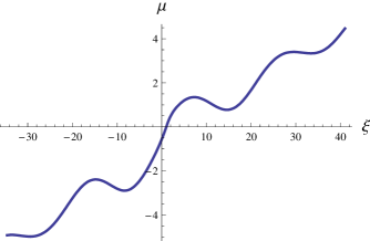
Figure 1: An example for the Theorem 4.1

We have the following extension of the results of D.G. de Figueiredo and W.-M. Ni [7] and R. Iannacci et al [8], which does not require that $\mu=0$.

Theorem 4.2

In addition to the conditions of the Theorem 4.1, assume that for some constants $c_{0}>0$ and $p>\frac{3}{2}$

(4.10) $$ug(u)>c_{0}|u|^{p},\;\;\mbox{for all $u>0$ ($u<0$)}\,.$$

Then for the problem (4.5) we have $\lim_{\xi_{1}\rightarrow\infty}\mu(\xi_{1})=\infty$ ($\,\lim_{\xi_{1}\rightarrow-\infty}\mu(\xi_{1})=-\infty$).

Proof:    Assume that (4.10) holds for $u>0$. By the Theorem 4.1, $\mu(\xi_{1})>0$ for $\xi_{1}$ large. Assume, on the contrary, that $\mu(\xi_{1})$ is bounded along some sequence of $\xi_{1}$’s, which tends to $\infty$. Writing $u=\xi_{1}\varphi_{1}+U$, we conclude from the line following (4.4) that

(4.11) $$\int_{\Omega}U^{2}\,dx\leq c_{1}\xi_{1}+c_{2},\;\;\mbox{for some constants $c_{1}>0$ and $c_{2}>0$}\,.$$

We have

$$\mu_{1}=\int_{\Omega}g(\xi_{1}\varphi_{1}+U)\varphi_{1}\,dx=\int_{\Omega}\left(g(\xi_{1}\varphi_{1}+U)-g(\xi_{1}\varphi_{1})\right)\varphi_{1}\,dx+\int_{\Omega}g(\xi_{1}\varphi_{1})\varphi_{1}\,dx\,.$$

Using the mean value theorem, the estimate (4.11), and the condition (4.10), we estimate

$$\mu_{1}>c_{3}{\xi_{1}}^{p-1}-c_{4}{\xi_{1}}^{1/2}-c_{5}\,,$$

with some positive constants $c_{3}$, $c_{4}$ and $c_{5}$. It follows that $\mu(\xi_{1})$ gets large along our sequence, a contradiction. $\diamondsuit$

Bounded perturbations at resonance are much easier to handle. For example, we have the following result.

Theorem 4.3

Assume that $g(u)\in C^{1}(R)$ is a bounded function, which satisfies the condition (4.6), and in addition,

$$\lim_{u\rightarrow\pm\infty}g(u)=0\,.$$

There is a continuous curve of solutions of (4.5): $(u(\xi_{1}),\mu_{1}(\xi_{1}))$, $u\in H^{2}(\Omega)\cap H^{1}_{0}(\Omega)$, with $-\infty<\xi_{1}<\infty$, and $\int_{\Omega}u(\xi_{1})\varphi_{1}\,dx=\xi_{1}$. This curve exhausts the solution set of (4.5). Moreover, there are constants $\mu_{-}<0<\mu_{+}$ so that the problem (4.5) has at least two solutions for $\mu\in(\mu_{-},\mu_{+})\setminus 0$, it has at least one solution for $\mu=\mu_{-}$, $\mu=0$ and $\mu=\mu_{+}$, and no solutions for $\mu$ lying outside of $(\mu_{-},\mu_{+})$.

Proof:    Follow the proof of the Theorem 4.1. Since $g(u)$ is bounded, we have a uniform in $\xi_{1}$ bound on $||U||_{C^{1}}$, see [7]. Since $\mu_{1}=\int_{\Omega}g(\xi_{1}\varphi_{1}+U)\varphi_{1}\,dx$, we conclude that for $\xi_{1}$ positive (negative) and large, $\mu_{1}$ is positive (negative) and it tends to zero as $\xi_{1}\rightarrow\infty$ ($\xi_{1}\rightarrow-\infty$). $\diamondsuit$

Example We have solved numerically the problem

$$u^{\prime\prime}+u+\frac{u}{2u^{2}+u+1}=\mu\sin x+\sin 2x,\;\;0<x<\pi,\;\;u(0)=u(\pi)=0\,.$$

The Theorem 4.3 applies. Write the solution as $u(x)=\xi\sin x+U(x)$, with $\int_{0}^{\pi}U(x)\sin x\,dx=0$. Then the solution curve $\mu=\mu(\xi)$ is given in Figure $2$. The picture shows that, say, for $\mu=-0.4$, the problem has exactly two solutions, while for $\mu=1$ there are no solutions.

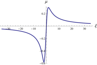
Figure 2: An example for the Theorem 4.3

We also have a result of Landesman-Lazer type, which also provides some additional information on the solution curve.

Theorem 4.4

Assume that the function $g(u)\in C^{1}(R)$ is bounded, it satisfies (4.7), and in addition, $g(u)$ has finite limits at $\pm\infty$, and

$$g(-\infty)<g(u)<g(\infty),\,\;\;\mbox{for all $u\in R$}\,.$$

Then there is a continuous curve of solutions of (4.5): $(u(\xi_{1}),\mu_{1}(\xi_{1}))$, $u\in H^{2}(\Omega)\cap H^{1}_{0}(\Omega)$, with $-\infty<\xi_{1}<\infty$, and $\int_{\Omega}u(\xi_{1})\varphi_{1}\,dx=\xi_{1}$. This curve exhausts the solution set of (4.5), and $\lim_{\xi_{1}\rightarrow\pm\infty}\mu_{1}(\xi_{1})=g(\pm\infty)\int_{\Omega}\varphi_{1}\,dx$. I.e., the problem (4.5) has a solution if and only if

$$g(-\infty)\int_{\Omega}\varphi_{1}\,dx<\mu<g(\infty)\int_{\Omega}\varphi_{1}\,dx\,.$$

Proof:    Follow the proof of the Theorem 4.1. Since $g(u)$ is bounded, we have a uniform bound on $U$, when we do the continuation in $\xi_{1}$. Hence $\mu_{1}\rightarrow g(\pm\infty)\int_{\Omega}\varphi_{1}\,dx$, as $\xi_{1}\rightarrow\pm\infty$, and by continuity of $\mu_{1}(\xi_{1})$, the problem (4.5) is solvable for all $\mu_{1}$’s lying between these limits. $\diamondsuit$

Example We have solved numerically the problem

$$u^{\prime\prime}+u+\frac{u}{\sqrt{u^{2}+1}}=\mu\sin x+5\sin 2x-\sin 10x,\;\;0<x<\pi,\;\;u(0)=u(\pi)=0\,.$$

The Theorem 4.4 applies. Write the solution as $u(x)=\xi\sin x+U(x)$, with $\int_{0}^{\pi}U(x)\sin x\,dx=0$. Then the solution curve $\mu=\mu(\xi)$ is given in Figure $3$. It confirms that $\lim_{\xi_{1}\rightarrow\pm\infty}\mu_{1}(\xi_{1})=\pm\frac{4}{\pi}$ ($\frac{4}{\pi}=\int_{0}^{\pi}\frac{2}{\pi}\,\sin x\,dx$).

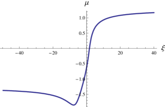
Figure 3: An example for the Theorem 4.4

One can append the following uniqueness condition (4.12) to all of the above results. For example, we have the following result.

Theorem 4.5

Assume that the conditions of the Theorem 4.1 hold, and in addition

(4.12) $$g^{\prime}(u)>0,\,\;\;\mbox{for all $u\in R$}\,.$$

Then

(4.13) $$\mu_{1}^{\prime}(\xi_{1})>0,\;\;\mbox{ for all $\xi_{1}\in R$}\,.$$

Proof:    Clearly, $\mu^{\prime}_{1}(\xi_{1})>0$ at least for some values of $\xi_{1}$. If (4.13) is not true, then $\mu^{\prime}_{1}(\xi^{0}_{1})=0$ at some $\xi^{0}_{1}$. Differentiate the equation (4.5) in $\xi_{1}$, set $\xi_{1}=\xi^{0}_{1}$, and denote $w=u_{\xi_{1}}|_{\xi_{1}=\xi^{0}_{1}}$, obtaining

$$\Delta w+\left(\lambda_{1}+g^{\prime}(u)\right)w=0\;\;\mbox{for $x\in\Omega$},$$

$$w=0\;\;\mbox{on $\partial\Omega$}.$$

Clearly, $w$ is not zero, since it has a non-zero projection on $\varphi_{1}$ ($U_{\xi_{1}}\in\varphi_{1}^{\perp}$). On the other hand, $w\equiv 0$, since by the assumption (4.7) we have $\lambda_{1}<\lambda_{1}+g^{\prime}(u)<\lambda_{2}$. $\diamondsuit$

Corollary 5

In addition to the conditions of this theorem, assume that the condition (4.10) holds, for all $u\in R$. Then for any $f(x)\in L^{2}(\Omega)$, the problem

$$\Delta u+\lambda_{1}u+g(u)=f(x)\,,\;\;\mbox{for $x\in\Omega$},\;\;u=0\;\;\mbox{on $\partial\Omega$}$$

has a unique solution $u(x)\in H^{2}(\Omega)\cap H^{1}_{0}(\Omega)$.

5 Resonance at higher eigenvalues

We consider the problem

(5.1) $$\Delta u+\lambda_{k}u+g(u)=f(x)\;\;\mbox{on $\Omega$},\;\;u=0\;\;\mbox{on $\partial\Omega$}\,,$$

where $\lambda_{k}$ is assumed to be a simple eigenvalue of $-\Delta$. We have the following extension of the result of D.G. de Figueiredo and W.-M. Ni [7] to the case of resonance at a non-principal eigenvalue.

Theorem 5.1

Assume that $g(u)\in C^{1}(R)$ is bounded, it satisfies (4.6), and

(5.2) $$g^{\prime}(u)\leq c_{0},\;\;\mbox{for all $u\in R$, and some $c_{0}>0$}\,,$$

(5.3) $$\liminf_{u\rightarrow\infty}g(u)>0,\;\;\limsup_{u\rightarrow-\infty}g(u)<0\,.$$

Assume that $f(x)\in L^{2}(\Omega)$ satisfies

(5.4) $$\int_{\Omega}f(x)\varphi_{k}(x)\,dx=0\,.$$

Then the problem (5.1) has a solution $u(x)\in H^{2}(\Omega)\cap H^{1}_{0}(\Omega)$.

Proof:    By (5.2) we may assume that $\lambda_{k}+g^{\prime}(u)\leq\lambda_{n+1}$ for some $n>k$. Expand $f(x)=\mu_{1}^{0}\varphi_{1}+\mu_{2}^{0}\varphi_{2}+\cdots+\mu_{n}^{0}\varphi_{n}+e(x)$, with $e(x)\in Span\{\varphi_{1},\ldots,\varphi_{n}\}^{\perp}$, and $u(x)=\xi_{1}\varphi_{1}+\xi_{2}\varphi_{2}+\cdots+\xi_{n}\varphi_{n}+U(x)$, with $U(x)\in Span\{\varphi_{1},\ldots,\varphi_{n}\}^{\perp}$. By (5.4), $\mu^{0}_{k}=0$. By the Theorem 3.1 for any $\xi=\left(\xi_{1},\ldots,\xi_{n}\right)$, one can find a unique $\mu=\left(\mu_{1},\ldots,\mu_{n}\right)$ for which the problem (3.1) has a solution of $n$-signature $\xi$, and we need to find a $\xi^{0}=\left(\xi^{0}_{1},\ldots,\xi^{0}_{n}\right)$, for which $\mu(\xi^{0})=\left(\mu^{0}_{1},\ldots,\mu^{0}_{k-1},0,\mu^{0}_{k+1},\ldots,\mu^{0}_{n}\right)$.

Multiplying the equation (5.1) by $\varphi_{i}$, and integrating we get

$$(\lambda_{k}-\lambda_{i})\xi_{i}+\int_{\Omega}g\left(\sum_{i=1}^{n}\xi_{i}\varphi_{i}+U\right)\varphi_{i}\,dx=\mu^{0}_{i},\;\;i=1,\ldots,k-1,k+1,\ldots n$$

$$\int_{\Omega}g\left(\sum_{i=1}^{n}\xi_{i}\varphi_{i}+U\right)\varphi_{k}\,dx=0\,.$$

We need to solve this system of equations for $\left(\xi_{1},\ldots,\xi_{n}\right)$. For that we set up a map $T:\left(\eta_{1},\ldots,\eta_{n}\right)\rightarrow\left(\xi_{1},\ldots,\xi_{n}\right)$, by calculating $\xi_{i}$ from

$$(\lambda_{k}-\lambda_{i})\xi_{i}=\mu^{0}_{i}-\int_{\Omega}g\left(\sum_{i=1}^{n}\eta_{i}\varphi_{i}+U\right)\varphi_{i}\,dx,\;\;i=1,\ldots,k-1,k+1,\ldots n$$

followed by

$$\xi_{k}=\eta_{k}-\int_{\Omega}g\left(\xi_{1}\varphi_{1}+\cdots+\xi_{k-1}\varphi_{k-1}+\eta_{k}\varphi_{k}+\xi_{k+1}\varphi_{k+1}+\cdots+\xi_{n}\varphi_{n}+U\right)\varphi_{k}\,dx\,.$$

Fixed points of this map provide solutions to our system of equations. By the Theorem 3.2, the map $T$ is continuous. Since $g(u)$ is bounded, $\left(\xi_{1},\ldots,\xi_{k-1},\xi_{k+1},\ldots,\xi_{n}\right)$ belongs to a bounded set. By (4.6) and (5.3), $\xi_{k}<\eta_{k}$ for $\eta_{k}>0$ and large, while $\xi_{k}>\eta_{k}$ for $\eta_{k}<0$ and $|\eta_{k}|$ large. Hence, the map $T$ maps a sufficiently large ball around the origin in $R^{n}$ into itself, and Brouwer’s fixed point theorem applies, giving us a fixed point of $T$. $\diamondsuit$

6 Numerical computation of solutions

We describe numerical computation of solutions for the problem

(6.1) $$u^{\prime\prime}+u+g(u)=\mu\sin x+e(x),\;\;0<x<\pi,\;\;u(0)=u(\pi)=0\,,$$

whose linear part is at resonance. We assume that $\int_{0}^{\pi}e(x)\sin x\,dx=0$. Writing $u(x)=\xi\sin x+U(x)$, with $\int_{0}^{\pi}U(x)\sin x\,dx=0$, we shall compute the solution curve of (6.1): $(u(\xi),\mu(\xi))$. (I.e., we write $\xi$, $\mu$ instead of $\xi_{1}$, $\mu_{1}$.) We shall use Newton’s method to perform continuation in $\xi$.

Our first task is to implement the “linear solver”, i.e., the numerical solution of the following problem: given any $\xi\in R$, and any functions $a(x)$ and $f(x)$, find $u(x)$ and $\mu$ solving

(6.2) $$u^{\prime\prime}+a(x)u=\mu\sin x+f(x),\;\;0<x<\pi\,,$$

$$u(0)=u(\pi)=0\,,$$

$$\int_{0}^{\pi}u(x)\sin x\,dx=\xi\,.$$

The general solution of the equation (6.2) is of course

$$u(x)=Y(x)+c_{1}u_{1}(x)+c_{2}u_{2}(x)\,,$$

where $Y(x)$ is any particular solution, and $u_{1}$,$u_{2}$ are two solutions of the corresponding homogeneous equation

(6.3) $$u^{\prime\prime}+a(x)u=0,\;\;0<x<\pi\,.$$

We shall use $Y=\mu Y_{1}+Y_{2}$, where $Y_{1}$ solves

$$u^{\prime\prime}+a(x)u=\sin x,\;\;u(0)=0,\;\;u^{\prime}(0)=1\,,$$

and $Y_{2}$ solves

$$u^{\prime\prime}+a(x)u=f(x),\;\;u(0)=0,\;\;u^{\prime}(0)=1\,.$$

Let $u_{1}(x)$ be the solution of (6.3) with $u(0)=0$, $u^{\prime}(0)=1$, and let $u_{2}(x)$ be any solution of (6.3) with $u_{2}(0)\neq 0$. The condition $u(0)=0$ implies that $c_{2}=0$, i.e., there is no need to compute $u_{2}(x)$, and we have

(6.4) $$u(x)=\mu Y_{1}(x)+Y_{2}(x)+c_{1}u_{1}(x)\,.$$

We used the NDSolve command in Mathematica to calculate $u_{1}$, $Y_{1}$ and $Y_{2}$. Mathematica not only solves differential equations numerically, but it returns the solution as an interpolated function of $x$, practically indistinguishable from an explicitly defined function.The condition $u(\pi)=0$ and the last line in (6.2) imply that

$$\mu Y_{1}(\pi)+c_{1}u_{1}(\pi)=-Y_{2}(\pi)\,,$$

$$\mu\int_{0}^{\pi}Y_{1}(x)\sin x\,dx+c_{1}\int_{0}^{\pi}u_{1}(x)\sin x\,dx=\xi-\int_{0}^{\pi}Y_{2}(x)\sin x\,dx\,,$$

Solving this system for $\mu$ and $c_{1}$, and using them in (6.4), we obtain the solution of (6.2).

Turning to the problem (6.1), we begin with an initial $\xi_{0}$, and using a step size $\Delta\xi$, on a mesh $\xi_{i}=\xi_{0}+i\Delta\xi$, $i=1,2,\ldots,nsteps$, we compute the solution of (6.1), satisfying $\int_{0}^{\pi}u(x)\sin x\,dx=\xi_{i}$, by using Newton’s method. Namely, assuming that the iterate $u_{n}(x)$ is already computed, we linearize the equation (6.1) at it, i.e., we solve the problem (6.2) with $a(x)=1+g^{\prime}(u_{n}(x))$, $f(x)=-g(u_{n}(x))+g^{\prime}(u_{n}(x))u_{n}(x)+e(x)$, and $\xi=\xi_{i}$. After several iterations, we compute $(u(\xi_{i}),\mu(\xi_{i}))$. We found that two iterations of Newton’s method, coupled with $\Delta\xi$ not too large (e.g., $\Delta\xi=0.5$), were sufficient for accurate computation of the solution curves. To start Newton’s iterations, we used $u(x)$ computed at the preceding step, i.e., $u(\xi_{i-1})$.

We have verified our numerical results by an independent calculation. Once a solution of (6.1) was computed at some $\xi_{i}$, we took its initial data $u(0)=0$ and $u^{\prime}(0)$, and computed numerically the solution of the equation in (6.1) with this initial data, let us call it $v(x)$ (using the NDSolve command). We always had $v(\pi)=0$ and $\int_{0}^{\pi}v(x)\sin x\,dx=\xi_{i}$.

References

[1]
H. Amann and P. Hess, A multiplicity result for a class of elliptic boundary value problems, Proc. Roy. Soc. Edinburgh Sect. A84, no. 1-2, 145-151 (1979).
[2]
A. Ambrosetti and G. Prodi, On the inversion of some differentiable mappings with singularities between Banach spaces, Ann. Mat. Pura Appl.93 (4), 231-246 (1972).
[3]
A. Ambrosetti and G. Prodi, A Primer of Nonlinear Analysis. Cambridge Studies in Advanced Mathematics, 34. Cambridge University Press, Cambridge, (1993).
[4]
M. S. Berger and E. Podolak, On the solutions of a nonlinear Dirichlet problem, Indiana Univ. Math. J.24, 837-846 (1974/75).
(1993).
[5]
M.G. Crandall and P.H. Rabinowitz, Bifurcation, perturbation of simple
eigenvalues and linearized stability, Arch. Rational Mech. Anal.52, 161-180 (1973).
[6]
L. Evans, Partial Differential Equations. Graduate Studies in Mathematics, 19. American Mathematical Society, Providence, RI, 1998.
[7]
D.G. de Figueiredo and W.-M. Ni, Perturbations of second order linear elliptic problems by nonlinearities without Landesman-Lazer condition, Nonlinear Anal.3 no. 5, 629-634 (1979).
[8]
R. Iannacci, M.N. Nkashama and J.R. Ward, Jr, Nonlinear second order elliptic partial differential equations at resonance, Trans. Amer. Math. Soc.311, no. 2, 711-726 (1989).
[9]
P. Korman,
A global solution curve for a class of periodic problems, including the pendulum equation,
Z. Angew. Math. Phys. (ZAMP) 58 no. 5, 749-766 (2007).
[10]
P. Korman, Curves of equiharmonic solutions, and ranges of nonlinear equations, Adv. Differential Equations14, no. 9-10, 963-984 (2009).
[11]
P. Korman, Global solution curves for boundary value problems, with linear part at resonance, Nonlinear Anal.71, no. 7-8, 2456-2467 (2009).
[12]
E.M. Landesman and A.C. Lazer, Nonlinear perturbations of linear elliptic
boundary value problems at resonance, J. Math. Mech.19, 609-623 (1970).
[13]
A.C. Lazer and P. J. McKenna, On the number of solutions of a nonlinear Dirichlet problem, J. Math. Anal. Appl.84, no. 1, 282-294 (1981).
[14]
L. Nirenberg, Topics in Nonlinear Functional Analysis, Courant Institute Lecture Notes, Amer. Math. Soc. (1974).