Longitudinal and transverse structure functions
in high Reynolds-number magneto-hydrodynamic turbulence

Abstract

We investigate the scaling behavior of longitudinal and transverse structure functions in homogeneous and isotropic magneto-hydrodynamic (MHD) turbulence by means of an exact hierarchy of structure function equations as well as by direct numerical simulations of two- and three-dimensional MHD turbulence. In particular, rescaling relations between longitudinal and transverse structure functions are derived and utilized in order to compare different scaling behavior in the inertial range. It is found that there are no substantial differences between longitudinal and transverse structure functions in MHD turbulence. This finding stands in contrast to the case of hydrodynamic turbulence which shows persistent differences even at high Reynolds numbers. We propose a physical picture that is based on an effective reduction of pressure contributions due to local regions of same magnitude and alignment of velocity and magnetic field fluctuations. Finally, our findings underline the importance of the pressure term for the actually observed scaling differences in hydrodynamic turbulence.

high Reynolds-number turbulence, magneto-hydrodynamics, structure functions, direct numerical simulations

1 Introduction

The question whether longitudinal and transverse structure functions posses different scaling behavior in highly turbulent flows is still an open and unsolved problem. Symmetry considerations [1] of the underlying Navier-Stokes equation suggest no difference in scaling behavior. However, experimental data [2, 3, 4] and high resolution numerical simulations [5, 6, 7, 8, 9] show a consistent difference between longitudinal and transverse structure functions. So far it is absolutely not clear what the cause of this observation is and possible explanations include a remaining small-scale anisotropy of the flow [10, 11] or a finite Reynolds number effect [12]. Thus a natural question and approach is to ask whether these differences between longitudinal and transverse structure functions exist or vanish in other turbulent systems in order to better understand and identify a possible cause. For instance, it was shown in the context of two-dimensional electron magneto-hydrodynamics [13] that the differences between longitudinal and transverse structure functions in the direct cascade range decreased with increasing Reynolds number.

In this paper we investigate the behavior of longitudinal and transverse structure functions in the context of magneto-hydrodynamic (MHD) turbulence. The motivation for looking at MHD turbulence arose from the known fact that current and vortex sheets play a key role for the understanding of intermittency in this particular flow. Since sheets represent quite anisotropic structures compared to vortex filaments as their hydrodynamic counterparts, the hope was to attribute the different scaling of longitudinal and transverse structure functions to the nature of the dissipative structures. It turned out that this statement is correct but in a way that was not anticipated and which is counterintuitive at first glance. The result of this paper is that there is no substantial difference longitudinal and transverse structure functions in the inertial range of high Reynolds number MHD flows. Moreover, this observation can be attributed to regions of preferential alignment of the magnetic and the velocity field which result in an effective depletion of pressure contributions. In reverse, these results also open up the way for a better understanding of the problem in hydrodynamic turbulence. The outline of the paper is as follows: First-of-all, we derive a hierarchy of structure function relations from the basic MHD equations, a rather technical part in section 2 which will be accompanied by A to G. These relations are then used in section 3, in order to derive rescaling relations between transverse and longitudinal structure functions along the lines of Grauer, Homann and Pinton [9]. The scaling behavior of longitudinal and transverse structure functions in direct numerical simulations of MHD turbulence will then be investigated with the help of these rescaling relations in section 4. The paper concludes with a simple examination of local regions of same magnitude and alignment of velocity and magnetic field contributions and their depleting effect on the total pressure.

2 Hierarchy of structure functions in MHD turbulence

The aim of this section is to establish relations between longitudinal and transverse structure functions in MHD turbulence similar to the ones that have been derived by Hill [12], Hill and Boratav [14] and Yakhot [15] for the case of hydrodynamic turbulence. To this end, we make use of the calculus of isotropic tensors in MHD turbulence introduced by Chandrasekhar [16]. We thus consider the MHD equations in the following form

$$\frac{\partial}{\partial t}u_{i}+u_{n}\frac{\partial}{\partial x_{n}}u_{i}-h_{n}\frac{\partial}{\partial x_{n}}h_{i} =-\frac{1}{\rho}\frac{\partial}{\partial x_{i}}\left(p+\frac{1}{2}\rho|{\bf h}|^{2}\right)+\nu\nabla^{2}_{\bf x}u_{i},$$ (1)

$$\frac{\partial}{\partial t}h_{i}+u_{n}\frac{\partial}{\partial x_{n}}h_{i}-h_{n}\frac{\partial}{\partial x_{n}}u_{i} =\lambda\nabla^{2}_{\bf x}h_{i},$$ (2)

where summation over equal indices is implied. Here, $p({\bf x},t)$ denotes the hydrodynamic pressure, $\rho$ the density, $\nu$ the kinematic viscosity and $\lambda$ the magnetic diffusivity of the fluid. In the following, the density of the fluid is set to one. Furthermore, it should be noted that in this convenient form of the MHD equations, the magnetic field ${\bf h}({\bf x},t)$ has the dimensions of a velocity [16]. From these equations (1-2), Chandrasekhar derived the MHD analogon of the Friedmann-Keller correlation function hierarchy [17] of hydrodynamic turbulence and made use of the calculus of isotropic tensors [18, 19] in order to derive, among other things, the corresponding von Kármán-Howarth equation of MHD turbulence.

In our approach, which is more concerned with the local isotropy of MHD turbulence, we introduce the velocity and magnetic field increments ${v}_{i}({\bf x},{\bf x}^{\prime},t)={u}_{i}({\bf x},t)-{u}_{i}({\bf x}^{\prime},t)=u_{i}-u_{i}^{\prime}$ and ${b}_{i}({\bf x},{\bf x}^{\prime},t)={h}_{i}({\bf x},t)-{h}_{i}({\bf x}^{\prime},t)=h_{i}-h_{i}^{\prime}$. The evolution equations for these increments can be derived in following a procedure devised by Hill [12] (see A for further details) and take the form

$$\qquad\frac{\partial}{\partial t}v_{i}+v_{n}\frac{\partial}{\partial r_{n}}v_{i}+U_{n}\frac{\partial}{\partial X_{n}}v_{i}-b_{n}\frac{\partial}{\partial r_{n}}b_{i}-H_{n}\frac{\partial}{\partial X_{n}}b_{i} = -P_{i}+\nu(\nabla_{\bf x}^{2}+\nabla_{{\bf x}^{\prime}}^{2})v_{i},$$ (3)

$$\qquad\frac{\partial}{\partial t}b_{i}+v_{n}\frac{\partial}{\partial r_{n}}b_{i}+U_{n}\frac{\partial}{\partial X_{n}}b_{i}-b_{n}\frac{\partial}{\partial r_{n}}v_{i}-H_{n}\frac{\partial}{\partial X_{n}}v_{i} = \lambda(\nabla_{\bf x}^{2}+\nabla_{{\bf x}^{\prime}}^{2})b_{i},$$ (4)

where we have introduced the mean fields ${U}_{i}=\frac{{u}_{i}+{u}_{i}^{\prime}}{2}$, ${H}_{i}=\frac{{h}_{i}+{h}_{i}^{\prime}}{2}$, and where we have switched to relative and center coordinates ${\bf r}={\bf x}-{\bf x}^{\prime}$ and ${\bf X}=\frac{{\bf x}+{\bf x}^{\prime}}{2}$. Furthermore, the total pressure gradient increment has been introduced according to

$$P_{i}=\frac{\partial}{\partial X_{i}}\left[p-p^{\prime}+\frac{1}{2}(|{\bf h}|^{2}-|{\bf h}^{\prime}|^{2})\right].$$ (5)

Eqs. (3) and (4) are the point of departure for the derivation of the structure function hierarchy, the main objective in this section. The usual procedure consists in multiplying Eqs. (3) and (4) by certain increment components and subsequently taking the ensemble average in order to make use of the assumption of homogeneity and isotropy.

Before we address this issue, however, we want to address certain implications of the additional magnetic field on the structure function procedure along the lines of Hill [12]. First-of-all, it is important to take notice of the influence of the mean magnetic field ${\bf H}$ in the increment evolution equations (3) and (4): In contrast to the mean velocity field ${\bf U}$, which can be removed in a system comoving with the mean velocity, the mean magnetic field will be present in all moment equations derived from the increment equations. The influence of these terms can only be removed by certain combinations of the moments in addition to the assumption of homogeneity. Furthermore, as far as the tensorial character of the moments derived from Eqs. (3) and (4) is concerned, we have to deal with certain statistical quantities that are not invariant under the full rotation group [18, 19]. This difference arises due to ${\bf h}$ being an axial vector which is unchanged under a reflexion, contrary to the true polar vector ${\bf u}$ which changes signs. Therefore, tensorial quantities that involve an odd number of magnetic field components exhibit a lack of mirror symmetry and are thus skew tensors. By contrast, an even number of magnetic field components leads to the usual tensorial forms encountered in hydrodynamic turbulence (see B for further discussion). Concerning the defining scalars of these tensors, an important restriction emerges from the incompressibility condition of the velocity and the magnetic field, i.e., $\frac{\partial}{\partial x_{i}}u_{i}({\bf x},t)=0$ and $\frac{\partial}{\partial x_{i}}h_{i}({\bf x},t)=0$. The incompressibility conditions give rise to a first relation between the transverse $S_{\,t\,t}^{{\bf v}{\bf v}}(r,t)$ and longitudinal $S_{r\,r}^{{\bf v}{\bf v}}(r,t)$ velocity (magnetic) field structure function of second order, namely

$$\qquad S_{\,t\,t}^{{\bf v}{\bf v}}(r,t)=\frac{1}{2r}\frac{\partial}{\partial r}\left(r^{2}S_{r\,r}^{{\bf v}{\bf v}}(r,t)\right)\qquad\textrm{and}\qquad S_{\,t\,t}^{{\bf b}{\bf b}}(r,t)=\frac{1}{2r}\frac{\partial}{\partial r}\left(r^{2}S_{r\,r}^{{\bf b}{\bf b}}(r,t)\right).$$ (6)

These relations are the well-known von Kármán-Howarth relations and are a direct consequence of the incompressibility, homogeneity and isotropy of the MHD flow discussed in B.1. The existence of such direct relations between higher-order longitudinal and transverse structure functions, however, is far less obvious. Therefore, we have to rely on structure function relations that are directly derived from the evolution equations of the increments, i.e., Eqs. (3) and (4).

A first evolution equation for the symmetric tensor of second order $\langle v_{i}v_{j}+b_{i}b_{j}\rangle$ is derived in E according to

$$\frac{\partial}{\partial t}\langle v_{i}v_{j}+b_{i}b_{j}\rangle+\frac{\partial}{\partial r_{n}}\langle v_{n}(v_{i}v_{j}+b_{i}b_{j})\rangle-\frac{\partial}{\partial r_{n}}\langle b_{n}(v_{i}b_{j}+v_{j}b_{i})\rangle$$ (7)

$$+\frac{\partial}{\partial X_{n}}\langle U_{n}(v_{i}v_{j}+b_{i}b_{j})\rangle-\frac{\partial}{\partial X_{n}}\langle H_{n}(v_{i}b_{j}+v_{j}b_{i})\rangle+\langle v_{i}P_{j}+v_{j}P_{i}\rangle$$

$$= 2\nu\left(\nabla^{2}_{\bf r}+\frac{1}{4}\nabla^{2}_{\bf X}\right)\langle v_{i}v_{j}\rangle-2\langle\epsilon_{i\,j}^{{\bf u}{\bf u}}\rangle+2\lambda\left(\nabla^{2}_{\bf r}+\frac{1}{4}\nabla^{2}_{\bf X}\right)\langle b_{i}b_{j}\rangle-2\langle\epsilon_{i\,j}^{{\bf h}{\bf h}}\rangle.$$

Here, we have introduced the tensors of the local energy dissipation rates

$$\epsilon_{i\,j}^{{\bf u}{\bf u}} = \nu\sum_{n}\left[\left(\frac{\partial u_{i}}{\partial x_{n}}\right)\left(\frac{\partial u_{j}}{\partial x_{n}}\right)+\left(\frac{\partial u_{i}^{\prime}}{\partial x_{n}^{\prime}}\right)\left(\frac{\partial u_{j}^{\prime}}{\partial x_{n}^{\prime}}\right)\right],$$ (8)

$$\epsilon_{i\,j}^{{\bf h}{\bf h}} = \lambda\sum_{n}\left[\left(\frac{\partial h_{i}}{\partial x_{n}}\right)\left(\frac{\partial h_{j}}{\partial x_{n}}\right)+\left(\frac{\partial h_{i}^{\prime}}{\partial x_{n}^{\prime}}\right)\left(\frac{\partial h_{j}^{\prime}}{\partial x_{n}^{\prime}}\right)\right].$$ (9)

Eq. (7) is the first equation in a chain of transport equations and couples to tensors of third order via the nonlinear terms. A further simplification of Eq. (7) arises from the assumption of homogeneity which enables us to neglect terms that involve a center derivative acting on the ensemble average, i.e., $\frac{\partial}{\partial X_{n}}\langle...\rangle=0$. At this stage of the hierarchy, pressure contributions also vanish on the basis of homogeneity [20].

The averaged equation of energy balance in MHD turbulence can be obtained from Eq. (7) in summing over equal $i=j$, which is performed in E. The latter equation can be used to derive the MHD analagon of Kolmogorov’s 4/5-law of hydrodynamic turbulence. In addition to the longitudinal velocity structure function of third order, the 4/5-law in MHD turbulence involves the mixed correlation function $C^{{\bf h}{\bf h}{\bf u}}_{i\,j\,,n}({\bf r},t)=\langle h_{i}h_{j}u_{n}^{\prime}\rangle$ that is symmetric in $i,j$ and the antisymmetric correlation function

$$C^{{\bf u}{\bf h}{\bf h}}_{\,i;j,n}({\bf r},t)=\langle(h_{j}u_{i}-u_{j}h_{i})h_{n}^{\prime}\rangle=C^{{\bf u}{\bf h}{\bf h}}_{\,r;t\,t}(r,t)\left(\frac{r_{j}}{r}\delta_{in}-\frac{r_{i}}{r}\delta_{jn}\right).$$ (10)

In the following, tensorial forms of the antisymmetric type (10) will be indicated by a semicolon between the antisymmetric indices. The notation of the correlation functions follows a similar approach than the notation used by Chandrasekhar in his seminal discussion of correlation functions in MHD turbulence [16]. Antisymmetric tensors such as (10) will be encountered throughout the entire structure function hierarchy in MHD turbulence and lead to modified scaling relations in comparison to the ordinary symmetric tensors encountered in hydrodynamics. This can be seen from the 4/5-law in MHD turbulence (see E.1) in the inertial range

$$S^{{\bf v}{\bf v}{\bf v}}_{r\,r\,r}\left(r\right)-12C^{{\bf h}{\bf h}{\bf u}}_{t\,\,t\,\,r}\left(r\right)-\frac{24}{r^{4}}\int_{0}^{r}\textrm{d}r^{\prime}~{}r^{\prime 3}C^{{\bf u}{\bf h}{\bf h}}_{\,r;t\,t}(r^{\prime})=-\frac{4}{5}\langle\varepsilon^{{\bf u}{\bf u}}+\varepsilon^{{\bf h}{\bf h}}\rangle r.$$ (11)

The corresponding averaged local energy dissipation rates $\langle\varepsilon^{{\bf u}{\bf u}}\rangle$ and $\langle\varepsilon^{{\bf h}{\bf h}}\rangle$ can be recovered from Eqs. (8,9), as it is further discussed in E. In the absence of the antisymmetric tensor, for instance in the case of a vanishing electromotive force in Eq. (10), we recover the relation established by Politano and Pouquet [21].

The next order equation relates structure functions of third and fourth order. It is also the first order which provides a relation between the longitudinal and transverse structure functions based on the MHD equations. By contrast, the von Kármán-Howarth relations (6) are a pure statement of the corresponding incompressibility conditions. Furthermore, in the next order of the hierarchy we have to deal for the first time with statistical quantities that contain the pressure gradient increment $P_{i}$. The evolution equation for the symmetric tensor of third order is derived in F and reads

$$\frac{\partial}{\partial t}\big{\langle}v_{i}v_{j}v_{k}+v_{i}b_{j}b_{k}+b_{i}v_{j}b_{k}+b_{i}b_{j}v_{k}\big{\rangle}+\frac{\partial}{\partial r_{n}}\big{\langle}v_{i}v_{j}v_{k}v_{n}-b_{i}b_{j}b_{k}b_{n}\big{\rangle}$$ (12)

$$+\frac{\partial}{\partial r_{n}}\langle v_{n}(v_{i}b_{j}b_{k}+b_{i}v_{j}b_{k}+b_{i}b_{j}v_{k})\rangle-\frac{\partial}{\partial r_{n}}\langle b_{n}(v_{i}v_{j}b_{k}+b_{i}v_{j}v_{k}+v_{i}b_{j}v_{k})\rangle$$

$$= -\left\langle(v_{i}v_{j}+b_{i}b_{j})P_{k}+(v_{i}v_{k}+b_{i}b_{k})P_{j}+(v_{j}v_{k}+b_{j}b_{k})P_{i}\right\rangle,$$

where dissipative terms have been neglected in the inertial range [14]. Obviously, this can only be a crude approximation since these terms contain the joint statistics of the the velocity (magnetic) field increment and the local energy dissipation rates (8,9), which are known to contribute even in the vicinity of $\nu,\lambda\rightarrow 0$. Nonetheless, for now we proceed in introducing the notations

$$S_{i\,j\,k\,n}^{{\bf v}{\bf v}{\bf v}{\bf v}}({\bf r},t) = \langle v_{i}v_{j}v_{k}v_{n}\rangle,$$ (13)

$$S_{i\,j\,k\,n}^{{\bf b}{\bf b}{\bf b}{\bf b}}({\bf r},t) = \langle b_{i}b_{j}b_{k}b_{n}\rangle,$$ (14)

$$S_{i\,j;k\,n}^{{\bf v}{\bf v}{\bf b}{\bf b}}({\bf r},t) = \langle v_{i}v_{j}b_{k}b_{n}-b_{i}b_{j}v_{k}v_{n}\rangle,$$ (15)

$$T_{ijk}({\bf r},t) = \left\langle(v_{i}v_{j}+b_{i}b_{j})P_{k}+(v_{i}v_{k}+b_{i}b_{k})P_{j}+(v_{j}v_{k}+b_{j}b_{k})P_{i}\right\rangle,$$ (16)

which enable us to rewrite Eq. (12) in shorter form as

$$\quad\frac{\partial}{\partial r_{n}}\left(S_{i\,j\,k\,n}^{{\bf v}{\bf v}{\bf v}{\bf v}}({\bf r},t)-S_{i\,j\,k\,n}^{{\bf b}{\bf b}{\bf b}{\bf b}}({\bf r},t)\right)$$ (17)

$$-\frac{\partial}{\partial r_{n}}\left(S_{i\,j;k\,n}^{{\bf v}{\bf v}{\bf b}{\bf b}}({\bf r},t)+S_{j\,k;i\,n}^{{\bf v}{\bf v}{\bf b}{\bf b}}({\bf r},t)+S_{i\,k;j\,n}^{{\bf v}{\bf v}{\bf b}{\bf b}}({\bf r},t)\right)=T_{ijk}({\bf r},t).$$

Here, the tensors in the first line are ordinary symmetric tensors of fourth order, described in D, whereas the mixed tensor possesses another tensorial form

$$S_{i\,j;k\,n}^{{\bf v}{\bf v}{\bf b}{\bf b}}({\bf r},t)=S_{r\,r;t\,t}^{{\bf v}{\bf v}{\bf b}{\bf b}}({r},t)\left(\frac{r_{i}r_{j}}{r^{2}}\delta_{kn}-\frac{r_{k}r_{n}}{r^{2}}\delta_{ij}\right),$$ (18)

since it is antisymmetric in exchanging $ij$ against $kn$. It can therefore be considered as the next-order equivalent tensor of Eq. (10). Inserting the corresponding tensors (D) yields

$$\frac{1}{r^{2}}\frac{\partial}{\partial r}\left[r^{2}\left(S_{r\,r\,r\,r}^{{\bf v}{\bf v}{\bf v}{\bf v}}({r})-S_{r\,r\,r\,r}^{{\bf b}{\bf b}{\bf b}{\bf b}}({r})\right)\right]-\frac{6}{r}\left(S_{r\,r\,t\,t}^{{\bf v}{\bf v}{\bf v}{\bf v}}({r})-S_{r\,r\,t\,t}^{{\bf b}{\bf b}{\bf b}{\bf b}}({r})-S_{r\,r;t\,t}^{{\bf v}{\bf v}{\bf b}{\bf b}}({r})\right)$$ (19)

$$=-T_{rrr}(r),$$

for the longitudinal structure functions and

$$\frac{1}{r^{4}}\frac{\partial}{\partial r}\left[r^{4}\left(S_{r\,r\,t\,t}^{{\bf v}{\bf v}{\bf v}{\bf v}}({r})-S_{r\,r\,t\,t}^{{\bf b}{\bf b}{\bf b}{\bf b}}({r})\right)\right]-\frac{4}{3r}\left(S_{t\,\,t\,\,t\,\,t}^{{\bf v}{\bf v}{\bf v}{\bf v}}({r})-S_{t\,\,t\,\,t\,\,t}^{{\bf b}{\bf b}{\bf b}{\bf b}}({r})\right)+\frac{\partial}{\partial r}S_{r\,r;t\,t}^{{\bf v}{\bf v}{\bf b}{\bf b}}({r})$$ (20)

$$=-T_{rtt}(r),$$

for the mixed structure functions.
These equations represent the generalization of the next-order structure function relations in hydrodynamic turbulence derived in [14] and [15] in the presence of a magnetic field. As in the hydrodynamic case the longitudinal and transverse structure functions of fourth order are coupled via the mixed terms $S_{r\,r\,t\,t}(r)$ in Eq. (19) and (20). Furthermore, the presence of the pressure contributions $T_{rrr}(r)$ and $T_{rtt}(r)$ in the inertial range are considered to be responsible for the persistent different scaling behavior between the longitudinal and transverse structure functions in hydrodynamic turbulence [9, 14, 22]. Nevertheless, Eq. (19) and (20) distinguish themselves from their hydrodynamic counterparts in several points: First-of-all, the presence of the antisymmetric tensor $S_{i\,j;k\,n}^{{\bf v}{\bf v}{\bf b}{\bf b}}({\bf r})(r)$ leads to novel terms, especially in the mixed velocity-magnetic structure function equation (20) that involves $S_{r\,r;t\,t}^{{\bf v}{\bf v}{\bf b}{\bf b}}({r})$ in a new differential relation compared to the other mixed structure functions. Furthermore, only differences between pure velocity and magnetic structure functions enter the relation, which can lead to cancellation effects, e.g., in the case of alignment solutions. In addition, the pressure contributions on the right-hand side of (19) and (20) include contributions from the magnetic pressure next to the hydrodynamic pressure which opens up the way to discuss the role of pressure in MHD turbulence via a local Bernoulli law along the lines of Gotoh and Nakano [22] for the case of hydrodynamic turbulence.

3 Rescaling relations between longitudinal and transverse structure functions

In this section, we briefly want to review rescaling relations between longitudinal and transverse structure functions of all orders that were derived recently [9]. We shall then proceed to motivate such rescaling relations for MHD turbulence, namely by means of Eqs. (19) and (20). The point of departure for hydrodynamic turbulence is the observation by Siefert and Peinke [23] that $S^{{\bf v}{\bf v}}_{r\,r}(r)$ is a smooth function of $r$ for which we can interpret the right-hand side of the von Kármán-Howarth relation (6) as the first two terms of a Taylor expansion around $r$

$$S^{{\bf v}{\bf v}}_{r\,r}\left(r+\frac{r}{2}\right)\approx S^{{\bf v}{\bf v}}_{r\,r}(r)+\frac{r}{2}\frac{\partial}{\partial r}S^{{\bf v}{\bf v}}_{r\,r}(r).$$ (21)

Here, we neglect terms of higher order under the assumption that $r/2$ is much smaller than the integral length scale $L$. In this approximation, the transverse structure function is simply the longitudinal structure function rescaled by the factor $3/2$ according to

$$S^{{\bf v}{\bf v}}_{t\,t}(r)\approx S^{{\bf v}{\bf v}}_{r\,r}\left(\frac{3}{2}r\right).$$ (22)

This procedure can be generalized for structure functions of the order $n$ in hydrodynamic turbulence [9], which is discussed at the example of the fourth order equations (19) and (20) in the hydrodynamic limit

$$\frac{1}{r^{2}}\frac{\partial}{\partial r}\left[r^{2}S_{r\,r\,r\,r}^{{\bf v}{\bf v}{\bf v}{\bf v}}({r})\right]-\frac{6}{r}S_{r\,r\,t\,t}^{{\bf v}{\bf v}{\bf v}{\bf v}}({r}) = -T_{rrr}(r),$$ (23)

$$\frac{1}{r^{4}}\frac{\partial}{\partial r}\left[r^{4}S_{r\,r\,t\,t}^{{\bf v}{\bf v}{\bf v}{\bf v}}({r})\right]-\frac{4}{3r}S_{t\,\,t\,\,t\,\,t}^{{\bf v}{\bf v}{\bf v}{\bf v}}({r}) = -T_{rtt}(r).$$ (24)

These two equations are solely related by the mixed term $S_{r\,r\,t\,t}^{{\bf v}{\bf v}{\bf v}{\bf v}}({r})$, in contrast to the MHD equations, where the antisymmetric mixed terms $S_{r\,r;t\,t}^{{\bf v}{\bf v}{\bf b}{\bf b}}({r})$ appear. The rescaling properties can be repeated under the neglect of the pressure terms, so that we obtain

$$3S_{r\,r\,t\,t}^{{\bf v}{\bf v}{\bf v}{\bf v}}({r}) \approx S_{r\,r\,r\,r}^{{\bf v}{\bf v}{\bf v}{\bf v}}({r})+\frac{r}{2}\frac{\partial}{\partial r}S_{r\,r\,r\,r}^{{\bf v}{\bf v}{\bf v}{\bf v}}({r})\approx S_{r\,r\,r\,r}^{{\bf v}{\bf v}{\bf v}{\bf v}}\left(\frac{3}{2}r\right),$$ (25)

$$\frac{1}{3}S_{t\,\,t\,\,t\,\,t}^{{\bf v}{\bf v}{\bf v}{\bf v}}({r}) \approx S_{r\,r\,t\,t}^{{\bf v}{\bf v}{\bf v}{\bf v}}({r})+\frac{r}{4}\frac{\partial}{\partial r}S_{r\,r\,t\,t}^{{\bf v}{\bf v}{\bf v}{\bf v}}({r})\approx S_{r\,r\,t\,t}^{{\bf v}{\bf v}{\bf v}{\bf v}}\left(\frac{5}{4}r\right),$$ (26)

which yields the transverse structure function of fourth order in terms of the rescaled longitudinal structure function of fourth order according to

$$S_{t\,\,t\,\,t\,\,t}^{{\bf v}{\bf v}{\bf v}{\bf v}}({r})\approx S_{r\,r\,r\,r}^{{\bf v}{\bf v}{\bf v}{\bf v}}\left({\frac{3}{2}\frac{5}{4}r}\right).$$ (27)

It is clear that neglecting the pressure terms in Eqs. (23) and (24) in combination with the corresponding Taylor expansions has to be treated with caution. Nevertheless, it has been shown [9] that the rescaling relations are an accurate method to map scales without altering the corresponding scaling behavior. It is therefore an essential tool for the investigation of possible different intermittency behavior of the longitudinal and transverse structure functions. In considering higher order structure function equations [12], a general relation between even order transverse structure function of order $n$ can be derived according to

$$S_{nt}^{n{\bf v}}({r})\approx S_{nr}^{n{\bf v}}\left(\frac{3}{2}\frac{5}{4}...\frac{n+1}{n}r\right)=S_{nr}^{n{\bf v}}\left(\frac{(n+1)!!}{n!!}r\right).$$ (28)

Turning to the case of MHD turbulence, the von Kármán-Howarth relation (6) suggests that Eq. (21) is also valid for the magnetic field structure functions of second order. The next order equations (19) and (20), however, are more complicated due to the additional appearance of the anti-symmetric tensor $S_{r\,r;t\,t}^{{\bf v}{\bf v}{\bf b}{\bf b}}({r})$. Nevertheless, assuming that the contribution of the latter are rather small, we can - in a first approximation - establish the same relation (27) between $S_{t\,\,t\,\,t\,\,t}^{{\bf v}{\bf v}{\bf v}{\bf v}}({r})-S_{t\,\,t\,\,t\,\,t}^{{\bf b}{\bf b}{\bf b}{\bf b}}({r})$ and $S_{r\,r\,r\,r}^{{\bf v}{\bf v}{\bf v}{\bf v}}({r})-S_{r\,r\,r\,r}^{{\bf b}{\bf b}{\bf b}{\bf b}}({r})$. Moreover, if velocity and magnetic structure functions possess a unique power law in the inertial range, it is appropriate to assume that the general rescaling relation (28) holds independently for velocity and magnetic structure functions of all orders, given that higher order relations similar to Eqs. (19) and (20) exist.

4 Direct Numerical Simulations of 3D MHD turbulence and comparison of longitudinal and transverse structure functions

In the previous section, we argued that rescaling relations of the form (28) apply for all even order velocity and magnetic structure functions. We have examined these relations in direct numerical simulations of 3D MHD turbulence. Tab. 1 summarizes the corresponding characteristic parameters of the simulations.

run	Reλ	$u_{rms}$	$h_{rms}$	$\langle\varepsilon^{{\bf u}{\bf u}}\rangle$	$\nu=\lambda$	$\eta$	$\tau_{\eta}$	$L$	$T_{L}$	$N^{3}$
3D NS	460	0.19	0	$3.6\cdot 10^{-3}$	$2.5\cdot 10^{-5}$	$1.45\cdot 10^{-3}$	0.083	1.85	9.9	$2048^{3}$
3D MHD	430	0.23	0.36	$1.2\cdot 10^{-2}$	$7\cdot 10^{-3}$	$2.3\cdot 10^{-3}$	0.078	2.75	6.5	$2048^{3}$

Table 1: Characteristic parameters of the direct numerical simulations of 3D MHD and hydrodynamic turbulence: Taylor-Reynolds number $\textrm{Re}_{\lambda}=\sqrt{\frac{15u_{rms}L}{\nu}}$, root mean square velocity $u_{rms}=\sqrt{\langle{\bf u}^{2}\rangle}$, root mean square magnetic field $h_{rms}=\sqrt{\langle{\bf h}^{2}\rangle}$, averaged kinetic energy dissipation rate $\langle\varepsilon^{{\bf u}{\bf u}}\rangle$, kinematic viscosity $\nu$ and magnetic diffusivity $\lambda$, dissipation length $\eta=\left(\frac{\nu^{3}}{\langle\varepsilon^{{\bf u}{\bf u}}\rangle}\right)^{1/4}$, dissipation time $\tau_{\eta}=\left(\frac{\nu}{\eta}\right)^{1/2}$, integral length scale $L=\frac{\left(\frac{1}{2}(u_{rms}^{2}+h_{rms}^{2})\right)^{\frac{3}{2}}}{\langle\varepsilon^{{\bf u}{\bf u}}\rangle+\langle\varepsilon^{{\bf h}{\bf h}}\rangle}$, large-eddy turn-over time $T_{L}=\frac{L}{u_{rms}}$ and resolution $N$. For the sake of completeness, the averaged magnetic energy dissipation rate $\langle\varepsilon^{{\bf h}{\bf h}}\rangle$ in the MHD simulations is $1.6\cdot 10^{-2}$.

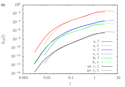
Figure 1: (a) Rescaled longitudinal and transverse structure functions in 3D MHD (green: magnetic field, blue: velocity field, Elsässer field ${\bf z}^{+}$: red) and hydrodynamic turbulence (black). The scales are mapped accurately via the rescaling relation (28). The hydrodynamic transverse structure function (dashed black line) possesses a slightly more intermittent character than the longitudinal structure function (straight black line) whereas the rescaled MHD structure functions do not show considerable differences.
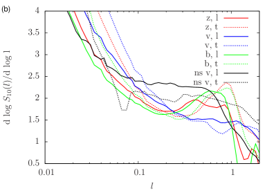
(b) Logarithmic derivatives of the structure functions from (a). Power law scaling should manifest itself as a flat curve.

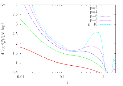
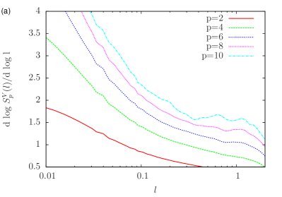
Figure 2: (a) Logarithmic derivative of the longitudinal velocity field structure functions of order $2-10$.
(b) Logarithmic derivative of the longitudinal magnetic field structure functions of order $2-10$.

As an example, Fig. 1 (a) shows the rescaling between longitudinal and transverse structure functions of order 10. The scales of the velocity field structure functions (blue) and the magnetic field structure functions (green) are mapped accurately onto each other. This is also true for the structure functions of the Elsässer field ${\bf z}^{+}({\bf x},t)={\bf u}({\bf x},t)+{\bf h}({\bf x},t)$. Furthermore, Fig. 1 shows no substantial difference between rescaled structure functions of order 10 in MHD turbulence. In opposition to the finding from hydrodynamic turbulence (see the black line in Fig. 1) which suggests that the rescaled transverse structure function possesses a slightly more intermittent character than the longitudinal one, we thus arrive at a somewhat contradictory conclusion: Although that structure functions in MHD turbulence are known to show a pronounced intermittency in comparison to their hydrodynamic counterparts [24], the differences in scaling behavior between longitudinal and transverse structure functions in MHD turbulence are less pronounced than in hydrodynamic turbulence. This becomes even more apparent from the logarithmic derivative plot of the longitudinal and transverse structure functions in Fig. 1 (b) which shows that the scaling exponents of the structure functions of order 10 in hydrodynamic turbulence lie above the ones in MHD turbulence. The latter fact is commonly attributed to the dissipative structures in MHD turbulence that consist mainly of vortex and current sheets and are believed to possess a more singular character than the vortex tubes in hydrodynamic turbulence [24]. Nevertheless, Fig. 1 shows that these geometric considerations are not an adequate explanation for the differences of scaling behavior between longitudinal and transverse structure functions in general.
The negative finding from MHD turbulence thus suggests that a more subtle mechanism is at the heart of the problem of the longitudinal and transverse structure function differences. Before we discuss such a mechanism on the basis of the pressure contributions that enter in Eqs. (19) and (20), it is in order to briefly discuss the notion of scaling in MHD turbulence in general. The logarithmic derivative plot in Fig. 1 (b) shows that a clear power law scaling of the structure functions is somehow hard to anticipate. In opposition, the structure functions from hydrodynamic turbulence (black) manifest themselves by rather flat curves (power law behavior) in the logarithmic derivative plot. Especially the magnetic longitudinal structure functions show a pronounced bump on larger scales $r$ and are thus missing a clear power law behavior as it can be seen from Fig. 2 (b). Moreover, the bump is increasing with increasing order of the structure function and seems to hint at the existence of two different power law behaviors in the inertial range. Since at this point, we are only interested in relative differences between longitudinal and transverse structure functions, we only take note of this problem of power laws in MHD turbulence and leave its evaluation to further work.

5 Alignment of dissipative structures and depletion of pressure

Apparently, the identical scaling behavior of the longitudinal and transverse structure functions in MHD turbulence discussed in the previous section is not directly related to the singular structures of the MHD flow. Therefore, we want to address a different mechanism that considers the influence of the pressure gradient on the longitudinal and transverse structure functions. In hydrodynamic turbulence, the relations (23) and (24) suggest that the scaling behavior of the longitudinal and transverse structure functions is altered solely by pressure contributions represented by $T_{rrr}(r)$ and $T_{rtt}(r)$.

run	Reλ	$u_{rms}$	$h_{rms}$	$\nu^{(2)}=\lambda^{(2)}$	dx	$\eta$	$\tau_{\eta}$	$L$	$T_{L}$	$N^{2}$
2D MHD	110-170	0.831	0.759	$2\cdot 10^{-10}$	$2,05\cdot 10^{-3}$	$1,64\cdot 10^{-3}$	0.037	4.741	5.705	$(3072)^{2}$

Table 2: Characteristic parameters of the numerical simulations: Taylor-Reynolds number $\textrm{Re}_{\lambda}=u_{rms}\left(\frac{L^{2}}{\nu^{(2)}(\langle\varepsilon^{{\bf u}{\bf u}}\rangle+\langle\varepsilon^{{\bf h}{\bf h}}\rangle)}\right)^{1/4}$, root mean square velocity $u_{rms}=\sqrt{\langle{\bf u}^{2}\rangle}$, root mean square magnetic field $h_{rms}=\sqrt{\langle{\bf h}^{2}\rangle}$, dissipation length $\eta=\left(\frac{(\nu^{(2)})^{3}}{\langle\varepsilon^{{\bf u}{\bf u}}\rangle}\right)^{\frac{1}{10}}$, dissipation time $\tau_{\eta}=\left(\frac{\nu^{(2)}}{\langle\varepsilon^{{\bf u}{\bf u}}\rangle^{2}}\right)^{\frac{1}{5}}$, integral length scale $L=\frac{\left(\frac{1}{2}(u_{rms}^{2}+h_{rms}^{2})\right)^{\frac{3}{2}}}{\langle\varepsilon^{{\bf u}{\bf u}}\rangle+\langle\varepsilon^{{\bf h}{\bf h}}\rangle}$ and large-eddy turn-over time $T_{L}=\frac{L}{u_{rms}}$.

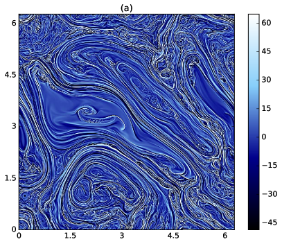
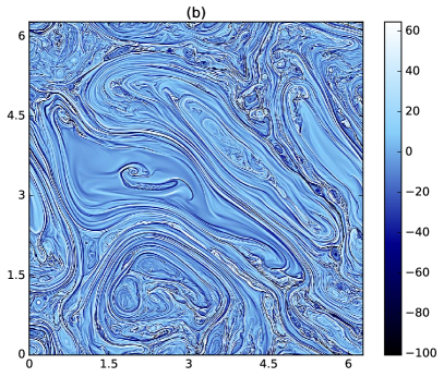
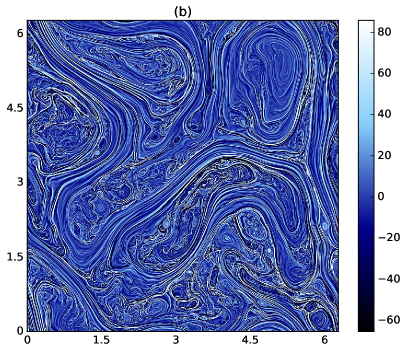
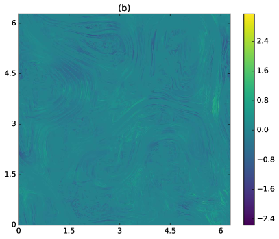
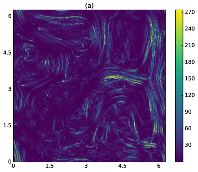
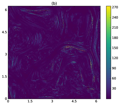
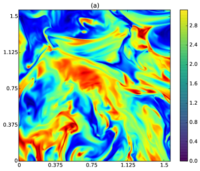
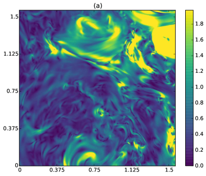
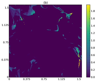
Figure 3: (a) Snapshot no. 1 of the vorticity field $\omega({\bf x},t)$ from direct numerical simulations of 2D MHD turbulence. (b) Same snapshot no. 1 of the current density $j({\bf x},t)$.

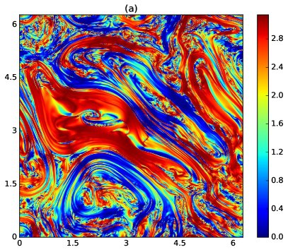
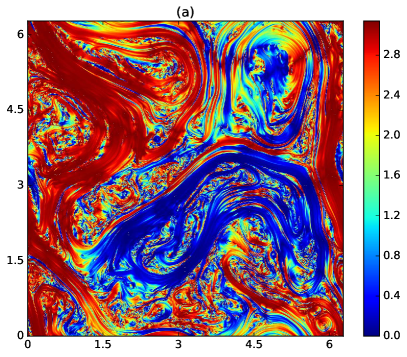
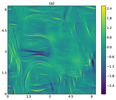
Figure 4: (a) Snapshot no. 1 of the alignment angle $\varphi({\bf x},t)$ between velocity field and magnetic field.
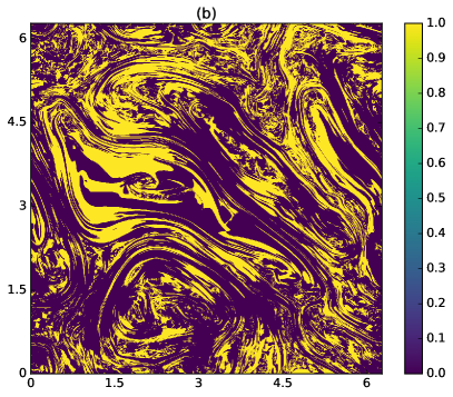
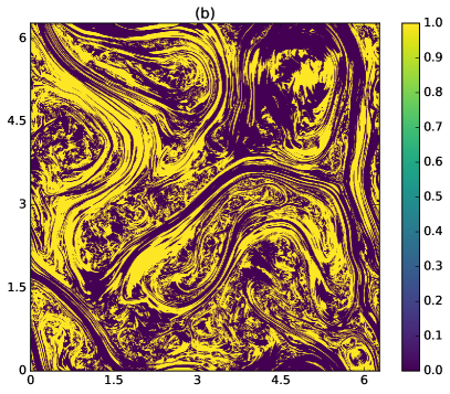
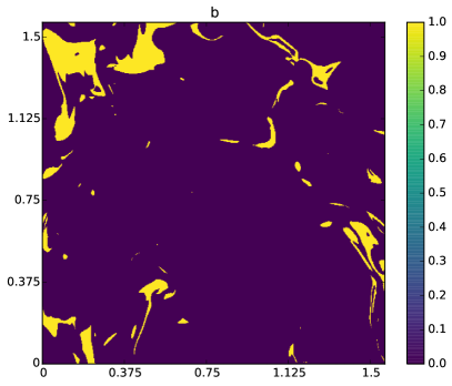
(b) Snapshot no. 1 of the filter function $\chi({\bf x},t)$ introduced in Eq. (31). The covered area is 35.33 per cent of the total area.

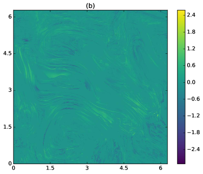
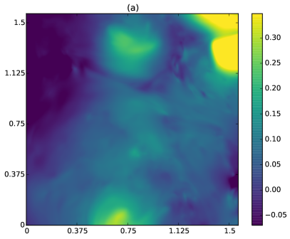
Figure 5: (a) Snapshot no. 1 of the total pressure field $p_{tot}({\bf x},t)$.
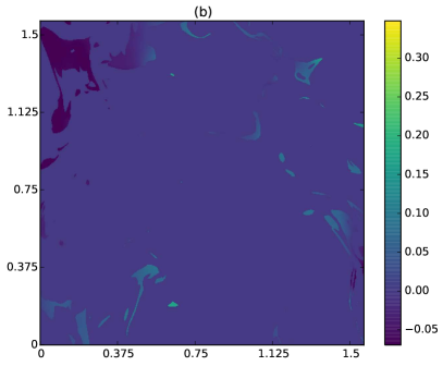
(b) Snapshot no. 1 of the filtered pressure field via the filter function $\chi({\bf x},t)$ from Eq. (31). The pressure field is effectively reduced.

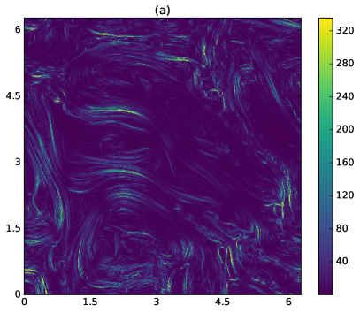
Figure 6: (a) Snapshot no. 1 of the norm of the total pressure gradient field $|\nabla p_{tot}({\bf x},t)|$.
(b) Snapshot no. 1 of the filtered norm of the pressure gradient field.

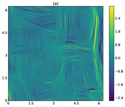
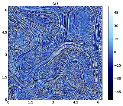
Figure 7: (a) Snapshot no. 2 of the vorticity field $\omega({\bf x},t)$ from direct numerical simulations of 2D MHD turbulence.
(b) Same snapshot no. 2 of the current density $j({\bf x},t)$.

Figure 8: (a) Snapshot no. 2 of the alignment angle $\varphi({\bf x},t)$ between velocity field and magnetic field. (b) Snapshot no. 2 of filter function $\chi({\bf x},t)$ in Eq. (31). The covered area is 44.57 per cent of the total area.

Figure 9: (a) Snapshot no. 2 of the total pressure field $p_{tot}({\bf x},t)$.
(b) Snapshot no. 2 of the filtered pressure field via the filter function $\chi({\bf x},t)$ from Eq. (31.) Again, the pressure field is effectively reduced.

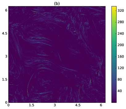
Figure 10: (a) Snapshot no. 2 of the norm of the total pressure gradient field $|\nabla p_{tot}({\bf x},t)|$.
(b) Snapshot no. 2 of the filtered norm of the pressure gradient field.

Consequently, the pressure contributions in MHD turbulence that enter on the r.h.s of Eqs. (19) and (20) have to be slightly milder than the ones in hydrodynamic turbulence. In order to quantitatively discuss this behavior it is convenient to consider the total pressure $p_{tot}({\bf x},t)=p({\bf x},t)+\frac{1}{2}|{\bf h}({\bf x},t)|^{2}$. Taking the divergence of Eq. (1) results in a Poisson equation for $p_{tot}({\bf x},t)$ that can be solved with the usual method of Green’s functions according to

$$p_{tot}({\bf x},t)=\frac{1}{4\pi}\int\frac{\textrm{d}{\bf x}^{\prime}}{|{\bf x}-{\bf x}^{\prime}|}\frac{\partial^{2}(u_{i}({\bf x}^{\prime},t)u_{j}({\bf x}^{\prime},t)-h_{i}({\bf x}^{\prime},t)h_{j}({\bf x}^{\prime},t))}{\partial x_{i}^{\prime}\partial x_{j}^{\prime}}.$$ (29)

As in hydrodynamic turbulence, the total pressure is thus determined nonlocally from the nonlinear terms in Eq. (1). Therefore, if the MHD flow possesses local regions of alignment and equal magnitude, i.e.,

$${\bf u}({\bf x},t)=\pm{\bf h}({\bf x},t),$$ (30)

this results in an effective depletion of pressure contributions that are mainly located in these regions due to the $1/|{\bf x}-{\bf x}^{\prime}|$ dependence in Eq. (29) (we refer the reader to the monograph [25] for a further discussion of these so-called equipartition solutions in MHD turbulence). As a consequence, the pressure gradient increment (5) that enters in the pressure contributions of Eqs. (19) and (20) is also reduced.

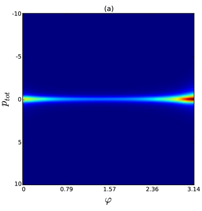
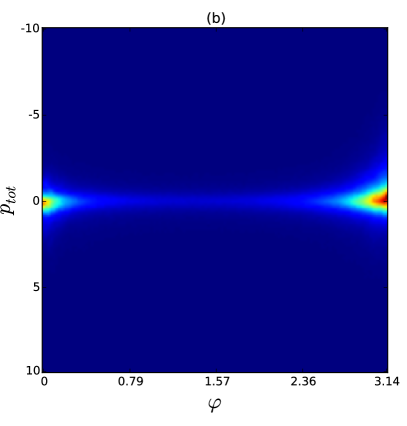
Figure 11: (a) Joint probability density function $PDF(p_{tot},\varphi)$ of pressure and alignment angle. Averages are performed over 700 snapshots. Vanishing pressure is found with high probability if the velocity and the magnetic field are aligned (anti-aligned). Note that in this particular time span of the simulations, anti-alignment occurs with a higher probability than alignment.
(b) Joint probability density function $PDF(p_{tot},\varphi)$ of pressure and alignment angle conditioned on the current density (20% of the maximum).

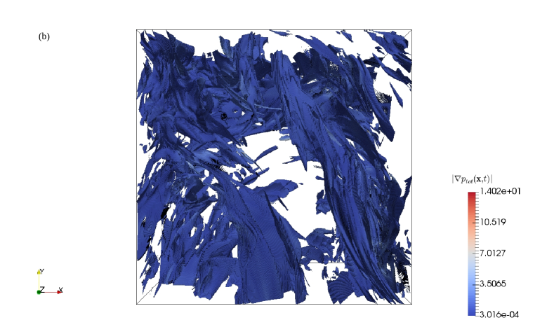
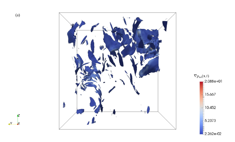
Figure 12: (a) Isosurface plot of the vorticity field $|\bm{\omega}({\bf x},t)|$ of a $512^{3}$-segment from direct numerical simulations of 3D MHD turbulence ($2048^{3}$). The isosurface lies at $0.35\,\omega_{max}$. The volumes are color coded with the magnitude of the total pressure gradient $|\nabla p_{tot}({\bf x},t)|$. (b) Isosurface plot of the filter function $\chi({\bf x},t)$ (31) of a $512^{3}$-segment from direct numerical simulations of 3D MHD turbulence ($2048^{3}$). The surface lies at 1 and is color coded with the magnitude of the total pressure gradient $|\nabla p_{tot}({\bf x},t)|$. The total pressure gradient vanishes in regions of alignment and same magnitude of velocity and magnetic field.

Figure 13: (a) Slice of the the alignment angle $\varphi({\bf x},t)$ between velocity field and magnetic field at constant $z=\pi/4$ for 3D MHD turbulence. (b) Slice of filter function $\chi({\bf x},t)$ in Eq. (31). The covered volume of the $512^{3}$-segment is 9.14 per cent.

Figure 14: (a) Slice of the pressure field at constant $z=\pi/4$ from Fig. 12 (b).
(b) Slice of the filtered pressure field via the filter function $\chi({\bf x},t)$ from Eq. (31).

Figure 15: (a) Slice of the norm of the pressure gradient field $|\nabla p_{tot}({\bf x},t)|$ at constant $z=\pi/4$ from Fig. 12 (b).
(b) Slice of the filtered norm of the pressure gradient field via the filter function $\chi({\bf x},t)$ from Eq. (31).

The described mechanism can thus be considered as a first explanation of the observations made in section 4. We emphasize that our alignment mechanism bears similarities with the phenomenological theory of scale-dependent alignment proposed by Boldyrev [26, 27] which is in accordance with experimentally obtained energy spectra of MHD turbulence. Boldyrev argued that small-scale turbulent eddies spontaneously develop alignment of magnetic and velocity field polarizations with respect to a large-scale magnetic field. The latter does not necessarily have to be an external magnetic field, but can also be apprehended as an effective magnetic field formed by the large scale vortical motions. Similar to the case of decaying MHD turbulence which ultimately reaches the equilibrium state in Eq. (30), the alignment causes a depletion of the nonlinearities in the MHD equations. In externally forced MHD turbulence, however, the tendency for dynamic alignment is reduced due to the energy flux across scales that preserves the nonlinear interactions. Therefore, at each scale $r$ of the energy cascade the alignment should reach a maximum that is consistent with the constant energy flux through this scale. In imposing the latter condition, Boldyrev derived the field-perpendicular energy spectrum according to $E(k_{\perp})\sim k_{\perp}^{-3/2}$.

In order to get a first idea and for reasons of graphical representation, we examine the impact of local regions of alignment on the pressure field by direct numerical simulations of forced 2D MHD turbulence. The characteristic parameters can be found in Table 2. Here, we made use of the concept of hyperviscosity by replacing $\nabla_{{\bf x}}^{2}\rightarrow(\nabla_{{\bf x}}^{2})^{2}$ in Eqs. (1) and (2) in order to attain higher Reynolds numbers and to extend the inertial range. As a first impression, we have depicted a snapshot of the vorticity $\omega({\bf x},t)=[\nabla\times{\bf u}({\bf x},t)]_{z}$ and the current density $j({\bf x},t)=[\nabla\times{\bf h}({\bf x},t)]_{z}$ in Fig. 3. The singular structures in the direct cascading range mainly consist of current and vortex sheets. The alignment angle $\varphi({\bf x},t)$ between ${\bf u}({\bf x},t)$ and ${\bf h}({\bf x},t)$ is depicted in Fig. 4 (a). It can already be seen that regions of preferential alignment and anti-alignment do in fact exist. In this particular snapshot no. 1 they occur in a nearly dipolar manner, for instance in the dipole on the left bottom. The clustering of like-signed alignment angles seems therefore to be in agreement with the arguments established by Boldyrev [26, 27]. The total pressure $p_{tot}({\bf x},t)$ of snapshot no. 1 is depicted in Fig. 5. and is mainly concentrated in dipolar boundary regions of the alignment angle, where flips out of the alignment (30) occur. This seems to support our hypothesis that pressure contributions are depleted in regions of alignment and comparable magnitude of the velocity and magnetic field. In order to further underline our hypothesis, we introduce a filter function

$$\chi({\bf x},t)=\left\{\begin{array}[]{ll}1&\textrm{where}~{}~{}|\cos(\varphi({\bf x},t))|>0.88~{}~{}\textrm{and}\\ &|u({\bf x},t)^{2}-h({\bf x},t)^{2}|<0.1\times\textrm{max}|u({\bf x},t)^{2}-h({\bf x},t)^{2}|,\\ 0&\textrm{ else}.\end{array}\right.$$ (31)

The filter function can roughly be interpreted as a measure of a deviation of ten per cent of the alignment relation (30). Applying this simple filter function to the total pressure in Fig. (5) shows that it is indeed depleted in regions of approximate alignment and equal magnitude. Since regions of maximal pressure contributions in Fig. 5 (b) are filtered, they can be assigned to regions where Eq. (30) is not fulfilled, i.e., ${\bf u}$ and ${\bf h}$ are not aligned. A second snapshot no. 2 is presented in Figs. 7-10. The snapshot no. 2 reveals an increased preference of aligned regions in comparison to snapshot no. 1. The area covered by the filter function is 44.57 per cent (snapshot no. 2) in comparison to 35.33 (snapshot no. 1). The alignment angle of snapshot no. 2 in Fig. 8 shows a pronounced dipole structure of alignment (anti-alignment). Pressure contributions in Fig. 9 -10 are also filtered to a great extend. In order to quantify and support our statement that the alignment of velocity and magnetic field is the cause for the absence of differences of longitudinal and transverse structure function scaling we constructed a two-dimensional histogram, where the joint probability density function of pressure and alignment angle is shown. Fig. 11 (a) demonstrates that with high probability the pressure is nearly zero if the alignment angle is either $0$ or $\pi$. Moreover, Fig. 11 (b) shows the same histogram but now conditioned on the current density above a threshold (20% of the maximum). Here, the vanishing of the pressure at angles $0$ and $\pi$ is even more pronounced and supports the above statement statement even stronger.

In the final part of this section, we extend our investigations to 3D MHD turbulence which was the basis of our findings in section 4. To this end, we have depicted an isosurface plot of the vorticity in Fig. 12 (a). The singular structures can be perceived as vortex sheets, in contrast to the hydrodynamic case that is dominated by tube-like vortical structures. Here, the plot consists of a $512^{3}$-segment of the full $2048^{3}$-box from a snapshot of the simulation in Tab. 1. Moreover, the volumes have been colored with the magnitude of the total pressure gradient. The total pressure gradient is seen to be small on strong vortex sheets. Fig. 12 (b) shows an isosurface plot of the filter function from Eq. (31). The isosurface has additionally been colored with the magnitude of the total pressure gradient. Again, the regions of preferential alignment and same magnitude of velocity and magnetic field directly correspond to regions of depleted total pressure gradient. A slice of the filter function at constant $z=\pi/4$ is depicted in Fig. 13 (b). The covered volume of the filter function is 9.14 per cent of the entire $512^{3}$-box, which is far less than in the 2D case. Fig. 14 (a) shows a slice for constant $z=\pi/4$ of the total pressure field from Fig. 12 (b). The filtered total pressure in Fig. 14 (b) and the filtered total pressure gradient Fig. 15 (b) supports our hypothesis that alignment regions effectively reduce pressure contributions.

6 Conclusion and Outlook

We derived a hierarchy of structure functions from the basic MHD equations. The deployed procedure yielded exact equations between longitudinal and transverse structure functions similar to the next order equations by Hill and Boratav [14] for the purely hydrodynamic limit case. Furthermore, neglecting the pressure contributions in these equations allowed us to establish rescaling relations between longitudinal and transverse structure functions in MHD turbulence. The latter were used to directly compare the scaling behavior of the longitudinal and transverse structure functions in the inertial range of direct numerical simulations of 3D MHD turbulence. In contrast to hydrodynamic turbulence, no clear scaling differences could be observed. This rather unexpected finding was explained by an effective reduction of the total pressure gradient due to regions of preferential alignment and same magnitude of velocity field and magnetic field fluctuations. In a first attempt, this potential mechanism was tested with the help of direct numerical simulations of 2D and 3D MHD turbulence. It could be shown that pressure contributions are indeed depleted in such regions of preferential equipartition. Further work will be dedicated to the identification of a similar mechanism in hydrodynamic turbulence.

Appendix A Derivation of the evolution equations for velocity and magnetic increments

The derivation of the evolution equations for velocity and magnetic field increments from the MHD equations (1) and (2) follows Hill’s procedure [12] for the case of hydrodynamic turbulence. We introduce the velocity and magnetic field increments

$${v}_{i}({\bf x},{\bf x}^{\prime},t) = {u}_{i}({\bf x},t)-{u}_{i}({\bf x}^{\prime},t),$$ (32)

$${b}_{i}({\bf x},{\bf x}^{\prime},t) = {h}_{i}({\bf x},t)-{h}_{i}({\bf x}^{\prime},t).$$ (33)

For brevity, let us denote $u_{i}({\bf x}^{\prime},t)=u_{i}^{\prime}$ and $h_{i}({\bf x}^{\prime},t)=h_{i}^{\prime}$. Furthermore, it is required that ${\bf x}$ and ${\bf x}^{\prime}$ have no relative motion so that terms like $\frac{\partial}{\partial x_{n}}u_{i}^{\prime}$ and $\frac{\partial}{\partial x_{n}^{\prime}}u_{i}$ vanish.
Subtracting the evolution equation of the velocity field (1) at point ${\bf x}^{\prime}$ from the same equation at point ${\bf x}$ and performing the same procedure for the induction equation (2) yields

$$\qquad\frac{\partial}{\partial t}v_{i}+u_{n}\frac{\partial}{\partial x_{n}}v_{i}+u_{n}^{\prime}\frac{\partial}{\partial x_{n}^{\prime}}v_{i}-h_{n}\frac{\partial}{\partial x_{n}}b_{i}-h_{n}^{\prime}\frac{\partial}{\partial x_{n}^{\prime}}b_{i}=-P_{i}+\nu(\nabla^{2}_{\bf x}+\nabla^{2}_{{\bf x}^{\prime}})v_{i},$$ (34)

$$\qquad\frac{\partial}{\partial t}b_{i}+u_{n}\frac{\partial}{\partial x_{n}}b_{i}+u_{n}^{\prime}\frac{\partial}{\partial x_{n}^{\prime}}b_{i}-h_{n}\frac{\partial}{\partial x_{n}}v_{i}-h_{n}^{\prime}\frac{\partial}{\partial x_{n}^{\prime}}v_{i}=\lambda(\nabla^{2}_{\bf x}+\nabla^{2}_{{\bf x}^{\prime}})b_{i},$$ (35)

where

$$P_{i}({\bf x},{\bf x}^{\prime},t)=\left(\frac{\partial}{\partial x_{i}}+\frac{\partial}{\partial x_{i}^{\prime}}\right)\left[p({\bf x},t)-p({\bf x}^{\prime},t)+\frac{1}{2}(|{\bf h}({\bf x},t)|^{2}-|{\bf h}({\bf x}^{\prime},t)|^{2})\right],$$ (36)

is the total pressure increment.
In the following, we introduce the mean velocity and magnetic fields

$$\qquad U_{i}({\bf x},{\bf x}^{\prime},t)=\frac{u_{i}({\bf x},t)+u_{i}({\bf x}^{\prime},t)}{2},$$ (37)

$$\qquad H_{i}({\bf x},{\bf x}^{\prime},t)=\frac{h_{i}({\bf x},t)+h_{i}({\bf x}^{\prime},t)}{2},$$ (38)

and perform a coordinate transform to relative and center coordinates according to

$$\qquad\quad~{}~{}{\bf r}={\bf x}-{\bf x}^{\prime}\qquad\textrm{and}\qquad{\bf X}=\frac{{\bf x}+{\bf x}^{\prime}}{2}.$$ (39)

The coordinate transform to relative and center coordinate implies the following relations for the derivatives

$$\frac{\partial}{\partial x_{i}}=\frac{1}{2}\frac{\partial}{\partial X_{i}}-\frac{\partial}{\partial r_{i}}\qquad\textrm{and}\qquad\frac{\partial}{\partial x_{i}^{\prime}}=\frac{1}{2}\frac{\partial}{\partial X_{i}}+\frac{\partial}{\partial r_{i}}.$$ (40)

In making use of these relations, we obtain the equations of motion for the velocity and the magnetic field increment

$$\frac{\partial}{\partial t}v_{i}+v_{n}\frac{\partial}{\partial r_{n}}v_{i}+U_{n}\frac{\partial}{\partial X_{n}}v_{i}-b_{n}\frac{\partial}{\partial r_{n}}b_{i}-H_{n}\frac{\partial}{\partial X_{n}}b_{i}=-\frac{\partial}{\partial X_{i}}P+\nu(\nabla_{\bf x}^{2}+\nabla_{{\bf x}^{\prime}}^{2})v_{i},$$

$$\frac{\partial}{\partial t}b_{i}+v_{n}\frac{\partial}{\partial r_{n}}b_{i}+U_{n}\frac{\partial}{\partial X_{n}}b_{i}-b_{n}\frac{\partial}{\partial r_{n}}v_{i}-H_{n}\frac{\partial}{\partial X_{n}}v_{i}=\lambda(\nabla_{\bf x}^{2}+\nabla_{{\bf x}^{\prime}}^{2})b_{i}.$$ (41)

By means of these conversions, the implication of homogeneity for the statistical interpretation of the increment equations (A) and (41) can be seen directly: If $\frac{\partial}{\partial X_{n}}$ acts on a statistical quantity, then $\frac{\partial}{\partial X_{n}}\langle...\rangle=0$, since this quantity should be independent of the rate of change with respect to the place where the measurement is performed [12].

Appendix B Structure functions of second order

As it has been pointed out by Chandrasekhar [16], the MHD equations provide the evolution equations for three different correlation functions of second order, namely $\langle u_{i}({\bf x},t)u_{j}({\bf x}^{\prime},t)\rangle$, $\langle h_{i}({\bf x},t)h_{j}({\bf x}^{\prime},t)\rangle$ and the cross helicity correlation function $\langle u_{i}({\bf x},t)h_{j}({\bf x}^{\prime},t)\rangle$. Under the assumption of homogeneity, the first two correlation functions possess the ordinary form of a tensor of order two, i.e., the tensorial form that is going to be introduced in Eq. (50). The third tensor, however, is a quantity that is not invariant under the full rotation group. This difference arises due to ${\bf h}$ being an axial vector which is unchanged under a reflexion whereas the true polar vector ${\bf u}$ changes signs. Due to this lack of mirror symmetry, the cross helicity correlation function possesses the following tensorial form

$$C_{i\,j}^{{\bf u}{\bf h}}({\bf r},t)=\langle u_{i}({\bf x},t)h_{j}({\bf x}^{\prime},t)\rangle=C^{{\bf u}{\bf h}}(r,t)\epsilon_{ijn}\frac{r_{n}}{r}.$$ (42)

In the following, our aim is to discuss a similar treatment for the structure functions of second order in MHD turbulence. To this end, let us consider the magnetic structure function of order two (the same treatment applies to the velocity structure function of order two):

$$S_{i\,j}^{{\bf b}{\bf b}}({\bf x},{\bf x}^{\prime},t)=\langle(h_{i}({\bf x},t)-h_{i}({\bf x}^{\prime},t))(h_{j}({\bf x},t)-h_{j}({\bf x}^{\prime},t))\rangle$$ (43)

$$=\langle h_{i}({\bf x},t)h_{j}({\bf x},t)\rangle+\langle h_{i}({\bf x}^{\prime},t)h_{j}({\bf x}^{\prime},t)\rangle-\langle h_{i}({\bf x},t)h_{j}({\bf x}^{\prime},t)\rangle-\langle h_{i}({\bf x}^{\prime},t)h_{j}({\bf x},t)\rangle$$

$$=2\langle h_{i}({\bf x},t)h_{j}({\bf x},t)\rangle-2\langle h_{i}({\bf x},t)h_{j}({\bf x}^{\prime},t)\rangle,$$

where homogeneity and isotropy were used in the last step, so that

$$\langle h_{i}({\bf x}^{\prime},t)h_{j}({\bf x}^{\prime},t)\rangle = \langle h_{i}({\bf x},t)h_{j}({\bf x},t)\rangle=C_{i\,j}^{{\bf h}{\bf h}}(0,t)$$

$$\langle h_{i}({\bf x},t)h_{j}({\bf x}^{\prime},t)\rangle = \langle h_{i}({\bf x}^{\prime},t)h_{j}({\bf x},t)\rangle=C_{i\,j}^{{\bf h}{\bf h}}({\bf r},t).$$ (44)

Therefore, the structure function $S_{i\,j}^{{\bf b}{\bf b}}({\bf r},t)$ can be written in terms of the correlation function $C_{i\,j}^{{\bf h}{\bf h}}({\bf r},t)$ according to

$$S_{i\,j}^{{\bf b}{\bf b}}({\bf r},t)=2(C_{i\,j}^{{\bf h}{\bf h}}(0,t)-C_{i\,j}^{{\bf h}{\bf h}}({\bf r},t)),$$ (45)

whereas the cross helicity structure function behaves in another way due to the lack of mirror symmetry

$$S_{i\,j}^{{\bf v}{\bf b}}({\bf x},{\bf x}^{\prime},t)=\langle(u_{i}({\bf x},t)-u_{i}({\bf x}^{\prime},t))(h_{j}({\bf x},t)-h_{j}({\bf x}^{\prime},t))\rangle$$ (46)

$$=\langle u_{i}({\bf x},t)h_{j}({\bf x},t)\rangle+\langle u_{i}({\bf x}^{\prime},t)h_{j}({\bf x}^{\prime},t)\rangle-\langle u_{i}({\bf x},t)h_{j}({\bf x}^{\prime},t)\rangle-\langle u_{i}({\bf x}^{\prime},t)h_{j}({\bf x},t)\rangle$$

$$=2\langle u_{i}({\bf x},t)h_{j}({\bf x},t)\rangle.$$

In the last step we made use of the assumption of homogeneity

$$\langle u_{i}({\bf x},t)h_{j}({\bf x},t)\rangle=\langle u_{i}({\bf x}^{\prime},t)h_{j}({\bf x}^{\prime},t)\rangle=C_{i\,j}^{{\bf u}{\bf h}}(0,t),$$ (47)

and

$$\langle u_{i}({\bf x},t)h_{j}({\bf x}^{\prime},t)\rangle=-\langle u_{i}({\bf x}^{\prime},t)h_{j}({\bf x},t)\rangle=C_{i\,j}^{{\bf u}{\bf h}}({\bf r},t).$$ (48)

This last relation is responsible for the different decomposition behavior of the second order tensor of the cross helicity structure function, which can be expressed in terms of the cross helicity correlation function according to

$$S_{i\,j}^{{\bf v}{\bf b}}({\bf r},t)=2C_{i\,j}^{{\bf u}{\bf h}}(0,t).$$ (49)

The cross helicity structure function thus becomes a purely local quantity.

B.1 The von Kármán-Howarth relation

In general we are interested in relations between longitudinal and transverse structure functions. Under the assumption of isotropy and homogeneity, the tensorial form of the second order magnetic structure function reads

$$S_{i\,j}^{{\bf b}{\bf b}}({\bf r},t)=(S_{r\,r}^{{\bf b}{\bf b}}(r,t)-S_{t\,\,t}^{{\bf b}{\bf b}}(r,t))\frac{r_{i}r_{j}}{r^{2}}+S_{t\,\,t}^{{\bf b}{\bf b}}(r,t)\delta_{ij},$$ (50)

where the subscript $rr$ denotes the longitudinal and $tt$ the transverse structure function. Eq. (45) implies that

$$\frac{\partial}{\partial r_{i}}S_{i\,j}^{{\bf b}{\bf b}}({\bf r},t)=0,$$ (51)

due to the incompressibility condition for the magnetic field. Inserting the tensorial form (50) yields

$$\frac{\partial}{\partial r_{i}}S_{i\,j}^{{\bf b}{\bf b}}({\bf r},t)$$

$$= \frac{\partial}{\partial r}(S_{r\,r}^{{\bf b}{\bf b}}(r,t)-S_{t\,\,t}^{{\bf b}{\bf b}}(r,t))\frac{r_{j}}{r}+\frac{2}{r}(S_{r\,r}^{{\bf b}{\bf b}}(r,t)-S_{t\,\,t}^{{\bf b}{\bf b}}(r,t))\frac{r_{j}}{r}+\frac{\partial}{\partial r}S_{t\,\,t}^{{\bf b}{\bf b}}(r,t)\frac{r_{j}}{r}=0,$$

where we made use of $\frac{\partial}{\partial r_{i}}=\frac{r_{i}}{r}\frac{\partial}{\partial r}$. We finally obtain a first relation between the longitudinal and the transverse structure function of second order

$$S_{t\,\,t}^{{\bf b}{\bf b}}(r,t)=\frac{1}{2r}\frac{\partial}{\partial r}\left(r^{2}S_{r\,r}^{{\bf b}{\bf b}}(r,t)\right),$$ (53)

which is known as the von Kármán-Howarth relation. The same relation holds also for the velocity structure function of second order whereas the cross helicity structure function bears no such relation.
Summing over equal $i$ and $j$ in (50) and making use of relation (53) yields

$$\langle v^{2}({r},t)\rangle=S_{r\,r}^{{\bf v}{\bf v}}(r,t)+2S_{t\,\,t}^{{\bf v}{\bf v}}(r,t)=\frac{1}{r^{2}}\frac{\partial}{\partial r}\left(r^{3}S_{r\,r}^{{\bf v}{\bf v}}(r,t)\right),$$ (54)

and similarly

$$\langle b^{2}({r},t)\rangle=S_{r\,r}^{{\bf b}{\bf b}}(r,t)+2S_{t\,\,t}^{{\bf b}{\bf b}}(r,t)=\frac{1}{r^{2}}\frac{\partial}{\partial r}\left(r^{3}S_{r\,r}^{{\bf b}{\bf b}}(r,t)\right),$$ (55)

which is needed for the averaged equation of energy balance in MHD turbulence (103).

Appendix C Structure functions of third order

The velocity structure function of third order reads

$$\quad S_{i\,j\,n}^{{\bf v}{\bf v}{\bf v}}({\bf x},{\bf x}^{\prime},t)=\langle(u_{i}({\bf x},t)-u_{i}({\bf x}^{\prime},t))(u_{j}({\bf x},t)-u_{j}({\bf x}^{\prime},t))(u_{n}({\bf x},t)-u_{n}({\bf x}^{\prime},t))\rangle.$$ (56)

Since $\langle u_{i}({\bf x},t)u_{j}({\bf x},t)u_{n}({\bf x},t)\rangle=0$, the structure function decomposes under the assumption of homogeneity and isotropy according to

$$S_{i\,j\,n}^{{\bf v}{\bf v}{\bf v}}({\bf r},t)=-2(C_{\,i\,j,n}^{{\bf u}{\bf u}{\bf u}}({\bf r},t)+C_{\,j\,n,i}^{{\bf u}{\bf u}{\bf u}}({\bf r},t)+2C_{\,n\,i,j}^{{\bf u}{\bf u}{\bf u}}({\bf r},t)),$$ (57)

where $C_{\,i\,j,n}^{{\bf u}{\bf u}{\bf u}}({\bf r},t)$ is a third order tensor that is symmetric in $ij$ and solenoidal in $n$, as it is described in [19]. It can thus solely be expressed by its longitudinal part

$$C_{\,i\,j,n}^{{\bf u}{\bf u}{\bf u}}({\bf r},t)= - \frac{r^{2}}{2}\frac{\partial}{\partial r}\left(\frac{C_{r\,r\,r}^{{\bf u}{\bf u}{\bf u}}(r,t)}{r}\right)\frac{r_{i}r_{j}r_{n}}{r^{3}}$$

$$+ \frac{1}{4r}\frac{\partial}{\partial r}\left(r^{2}C_{r\,r\,r}^{{\bf u}{\bf u}{\bf u}}(r,t)\right)\left(\frac{r_{i}}{r}\delta_{jn}+\frac{r_{j}}{r}\delta_{in}\right)-\frac{C_{r\,r\,r}^{{\bf u}{\bf u}{\bf u}}(r,t)}{2}\frac{r_{n}}{r}\delta_{ij}.$$

Inserting this tensorial form in Eq. (57) yields

$$\quad S_{i\,j\,n}^{{\bf v}{\bf v}{\bf v}}({\bf r},t)=3r^{2}\frac{\partial}{\partial r}\left(\frac{C_{r\,r\,r}^{{\bf u}{\bf u}{\bf u}}(r,t)}{r}\right)\frac{r_{i}r_{j}r_{n}}{r^{3}}-\frac{\partial}{\partial r}(rC_{r\,r\,r}^{{\bf u}{\bf u}{\bf u}}(r,t))\left(\frac{r_{n}}{r}\delta_{ij}+\frac{r_{i}}{r}\delta_{jn}+\frac{r_{j}}{r}\delta_{in}\right).$$

Now, we contract this tensor to a tensor of second order and obtain

$$\quad S_{r\,j\,n}^{{\bf v}{\bf v}{\bf v}}({\bf r},t) = \frac{r_{i}}{r}S_{i\,j\,n}^{{\bf v}{\bf v}{\bf v}}({\bf r},t)$$ (59)

$$= \left(r\frac{\partial}{\partial r}C_{r\,r\,r}^{{\bf u}{\bf u}{\bf u}}(r,t)-5C_{r\,r\,r}^{{\bf u}{\bf u}{\bf u}}(r,t)\right)\frac{r_{j}r_{n}}{r^{2}}-\frac{\partial}{\partial r}(rC_{r\,r\,r}^{{\bf u}{\bf u}{\bf u}}(r,t))\delta_{jn}.$$

Comparing this relation to the general form of a tensor of second order, for instance (50) gives

$$\quad S_{r\,t\,t}^{{\bf v}{\bf v}{\bf v}}({r},t) = -\frac{\partial}{\partial r}(rC_{r\,r\,r}^{{\bf u}{\bf u}{\bf u}}(r,t)),$$ (60)

$$\quad S_{r\,r\,r}^{{\bf v}{\bf v}{\bf v}}({r},t) = \left(r\frac{\partial}{\partial r}C_{r\,r\,r}^{{\bf u}{\bf u}{\bf u}}(r,t)-5C_{r\,r\,r}^{{\bf u}{\bf u}{\bf u}}(r,t)\right)+S_{r\,t\,t}^{{\bf v}{\bf v}{\bf v}}({r},t)=-6C_{r\,r\,r}^{{\bf u}{\bf u}{\bf u}}(r,t).$$ (61)

From these equations, a relation between the mixed and the longitudinal velocity structure function of third order can be derived as

$$S_{r\,t\,t}^{{\bf v}{\bf v}{\bf v}}({r},t)=\frac{1}{6}\frac{\partial}{\partial r}(rS_{r\,r\,r}^{{\bf v}{\bf v}{\bf v}}({r},t)).$$ (62)

Summing (59) over equal indices $j=n$ gives

$$S^{{\bf v}{\bf v}{\bf v}}({r},t)=\langle v_{r}(r,t){\bf v}(r,t)^{2}\rangle=S_{r\,r\,r}^{{\bf v}{\bf v}{\bf v}}({r},t)+2S_{r\,t\,t}^{{\bf v}{\bf v}{\bf v}}({r},t),$$ (63)

which can be rewritten with the relation (62) as

$$S^{{\bf v}{\bf v}{\bf v}}({r},t)=\frac{1}{3r^{3}}\frac{\partial}{\partial r}\left(r^{4}S^{{\bf v}{\bf v}{\bf b}}_{r\,r\,r\,}(r,t)\right).$$ (64)

This is the average which is needed for the averaged equation of energy balance in MHD turbulence (103).
The other average stems from the mixed third order tensor

$$S^{{\bf b}{\bf b}{\bf v}}_{i\,j\,n}\left({\bf r},t\right)-S^{{\bf v}{\bf b}{\bf b}}_{i\,j\,n}\left({\bf r},t\right)=U_{ijn}({\bf r},t)+H_{ijn}({\bf r},t),$$ (65)

from equation (100) and can be divided into

$$\qquad U_{ijn}({\bf r},t)=-2(-\langle h_{j}h_{n}u_{i}^{\prime}\rangle-\langle h_{i}h_{n}u_{j}^{\prime}\rangle+\langle h_{i}h_{j}u_{n}^{\prime}\rangle),$$ (66)

and

$$\qquad H_{ijn}({\bf r},t)=-2(\langle(u_{n}h_{j}-u_{j}h_{n})h_{i}^{\prime}\rangle+\langle(u_{n}h_{i}-u_{i}h_{n})h_{j}^{\prime}\rangle-\langle(u_{j}h_{i}+u_{i}h_{j})h_{n}^{\prime}\rangle).$$ (67)

Turning first to $U_{ijn}({\bf r},t)$, we have to evaluate correlation functions like $C^{{\bf h}{\bf h}{\bf u}}_{\,i\,j,n}({\bf r},t)=\langle h_{i}h_{j}u_{n}^{\prime}\rangle$. Since this tensor is again symmetric in $ij$ and solenoidal in $n$, it has the same tensorial form as $C^{{\bf u}{\bf u}{\bf u}}_{\,i\,j,n}({\bf r},t)=\langle u_{i}u_{j}u_{n}^{\prime}\rangle$ in Eq. (C) and can solely be expressed in terms of $C_{r\,r\,r}^{{\bf h}{\bf h}{\bf u}}(r,t)$

$$\qquad U_{ijn}({\bf r},t) = \left(C_{r\,r\,r}^{{\bf h}{\bf h}{\bf u}}(r,t)-r\frac{\partial}{\partial r}C_{r\,r\,r}^{{\bf h}{\bf h}{\bf u}}(r,t)\right)\frac{r_{i}r_{j}r_{n}}{r^{3}}$$

$$-C_{r\,r\,r}^{{\bf h}{\bf h}{\bf u}}(r,t)\left(\frac{r_{i}}{r}\delta_{jn}+\frac{r_{j}}{r}\delta_{in}\right)+\left(3C_{r\,r\,r}^{{\bf h}{\bf h}{\bf u}}(r,t)+r\frac{\partial}{\partial r}C_{r\,r\,r}^{{\bf h}{\bf h}{\bf u}}(r,t)\right)\frac{r_{n}}{r}\delta_{ij}.$$

This yields the following relations between the structure function $U_{ijn}(r,t)$ and the correlation function $C_{r\,r\,r}^{{\bf h}{\bf h}{\bf u}}(r,t)$

$$U_{rrr}(r,t) = 2C_{r\,r\,r}^{{\bf h}{\bf h}{\bf u}}(r,t),$$ (69)

$$U_{rtt}(r,t) = -C_{r\,r\,r}^{{\bf h}{\bf h}{\bf u}}(r,t),$$ (70)

$$U_{ttr}(r,t) = 3C_{r\,r\,r}^{{\bf h}{\bf h}{\bf u}}(r,t)+r\frac{\partial}{\partial r}C_{r\,r\,r}^{{\bf h}{\bf h}{\bf u}}(r,t).$$ (71)

For $H_{ijn}(r,t)$ we need the antisymmetric tensor

$$C^{{\bf u}{\bf h}{\bf h}}_{\,i;j,n}({\bf r},t)=\langle(h_{j}u_{i}-u_{j}h_{i})h_{n}^{\prime}\rangle=C^{{\bf u}{\bf h}{\bf h}}_{\,r;t\,t}(r,t)\left(\frac{r_{j}}{r}\delta_{in}-\frac{r_{i}}{r}\delta_{jn}\right).$$ (72)

and its symmetric counterpart

$$C^{{\bf u}{\bf h}{\bf h}}_{\,jn,i}({\bf r},t)=\langle(h_{j}u_{n}+u_{j}h_{n})h_{i}^{\prime}\rangle,$$ (73)

which again fulfills the same equation as $C_{\,i\,j,n}^{{\bf u}{\bf u}{\bf u}}({\bf r},t)$, namely (C).
We obtain

$$\qquad\qquad H_{ijn}({\bf r},t)= \left(C_{r\,r\,r}^{{\bf u}{\bf h}{\bf h}}(r,t)-r\frac{\partial}{\partial r}C_{r\,r\,r}^{{\bf u}{\bf h}{\bf h}}(r,t)\right)\frac{r_{i}r_{j}r_{n}}{r^{3}}$$ (74)

$$+ \left(\frac{1}{2r}\frac{\partial}{\partial r}(r^{2}C_{r\,r\,r}^{{\bf u}{\bf h}{\bf h}}(r,t))+2C^{{\bf u}{\bf h}{\bf h}}_{\,r;t\,t}(r,t)\right)\left(\frac{r_{i}}{r}\delta_{jn}+\frac{r_{j}}{r}\delta_{in}\right)$$

$$+ (-C_{r\,r\,r}^{{\bf u}{\bf h}{\bf h}}(r,t)-4C^{{\bf u}{\bf h}{\bf h}}_{\,r;t\,t}(r,t))\frac{r_{n}}{r}\delta_{ij}.$$

This yields the following relations

$$H_{rrr}(r,t) = 2C_{r\,r\,r}^{{\bf u}{\bf h}{\bf h}}(r,t),$$ (75)

$$H_{rtt}(r,t) = \frac{1}{2r}\frac{\partial}{\partial r}(r^{2}C_{r\,r\,r}^{{\bf u}{\bf h}{\bf h}}(r,t))+2C^{{\bf u}{\bf h}{\bf h}}_{\,r;t\,t}(r,t),$$ (76)

$$H_{ttr}(r,t) = -C_{r\,r\,r}^{{\bf u}{\bf h}{\bf h}}-4C^{{\bf u}{\bf h}{\bf h}}_{\,r;t\,t}(r,t).$$ (77)

We need the function $S^{{\bf b}{\bf b}{\bf v}}\left(r,t\right)-S^{{\bf v}{\bf b}{\bf b}}\left(r,t\right)$ for the averaged equation of energy balance in spherical coordinates.
By making use of

$$C_{r\,r\,r}^{{\bf h}{\bf h}{\bf u}}(r,t)=-2C_{t\,t\,r}^{{\bf h}{\bf h}{\bf u}}(r,t),$$ (78)

we get

$$S^{{\bf b}{\bf b}{\bf v}}\left(r,t\right)-S^{{\bf v}{\bf b}{\bf b}}\left(r,t\right) = \langle v_{r}(r,t)b^{2}(r,t)\rangle-2\langle b_{r}(r,t){\bf v}(r,t)\cdot{\bf b}(r,t)\rangle$$ (79)

$$= U_{rrr}(r,t)+2U_{ttr}(r,t)+H_{rrr}(r,t)+2H_{ttr}(r,t)$$

$$= -\frac{4}{r^{3}}\frac{\partial}{\partial r}(r^{4}C_{t\,\,t\,\,r}^{{\bf h}{\bf h}{\bf u}}(r,t))-8C^{{\bf u}{\bf h}{\bf h}}_{\,r;t\,t}(r,t).$$

Interestingly, the contributions from the symmetric correlation tensor $\langle(u_{j}h_{i}+u_{i}h_{j})h_{n}^{\prime}\rangle)$ vanish from this expression.

Appendix D Structure functions of fourth order

The tensor of fourth order, symmetric in all four indices is given by Monin and Yaglom [28] in Vol. II by formula (13.82). It has the form

$$S_{ijkn}({\bf r},t)=(S_{rrrr}(r,t)-6S_{rrtt}(r,t)+S_{tttt}(r,t))\frac{r_{i}r_{j}r_{k}r_{n}}{r^{4}}$$ (80)

$$+ (S_{rrtt}(r,t)-\frac{1}{3}S_{tttt}(r,t))\left[\frac{r_{i}r_{j}}{r^{2}}\delta_{kn}+\frac{r_{i}r_{k}}{r^{2}}\delta_{jn}+\frac{r_{i}r_{n}}{r^{2}}\delta_{jk}+\frac{r_{j}r_{k}}{r^{2}}\delta_{in}+\frac{r_{j}r_{n}}{r^{2}}\delta_{ik}+\frac{r_{k}r_{n}}{r^{2}}\delta_{ij}\right]$$

$$+ \frac{1}{3}S_{rrtt}(r,t)[\delta_{ij}\delta_{kn}+\delta_{ik}\delta_{jn}+\delta_{in}\delta_{jk}].$$

If we calculate its divergence we get a tensor of third order, whose tensorial form is given by Monin and Yaglom [28] in Vol. II by formula (13.80), therefore we obtain

$$\frac{\partial}{\partial r_{n}}S_{ijkn}({\bf r},t) = \left(\frac{\partial}{\partial r_{n}}S_{rrrn}({\bf r},t)-3\frac{\partial}{\partial r_{n}}S_{rttn}({\bf r},t)\right)\frac{r_{i}r_{j}r_{n}}{r^{3}}$$ (81)

$$+ \frac{\partial}{\partial r_{n}}S_{rttn}({\bf r},t)\left[\frac{r_{i}}{r}\delta_{jk}+\frac{r_{j}}{r}\delta_{ik}+\frac{r_{k}}{r}\delta_{ij}\right].$$

This tensorial form can be compared with the original calculations. We get

$$\frac{\partial}{\partial r_{n}}S_{rrrn}({\bf r},t)-3\frac{\partial}{\partial r_{n}}S_{rttn}({\bf r},t) = \left(\frac{\partial}{\partial r}+\frac{2}{r}\right)(S_{rrrr}(r,t)-6S_{rrtt}(r,t)+S_{tttt}(r,t))$$ (82)

$$+ \left(3\frac{\partial}{\partial r}-\frac{6}{r}\right)\left(S_{rrtt}(r,t)-\frac{1}{3}S_{tttt}(r,t)\right),$$

and

$$\frac{\partial}{\partial r_{n}}S_{rttn}({\bf r},t)=\left(\frac{\partial}{\partial r}+\frac{4}{r}\right)S_{rrtt}(r,t)-\frac{4}{3r}S_{tttt}(r,t).$$ (83)

The last equation has to be inserted into (82) in order to get the equation for the longitudinal structure function $\frac{\partial}{\partial r_{n}}S_{rrrn}({\bf r},t)$.
For the antisymmetric tensor

$$S_{i\,j;k\,n}^{{\bf v}{\bf v}{\bf b}{\bf b}}({\bf r},t)=\langle v_{i}v_{j}b_{k}b_{n}-b_{i}b_{j}v_{k}v_{n}\rangle=S_{r\,r;t\,t}^{{\bf v}{\bf v}{\bf b}{\bf b}}({r},t)\left(\frac{r_{i}r_{j}}{r^{2}}\delta_{kn}-\frac{r_{k}r_{n}}{r^{2}}\delta_{ij}\right).$$ (84)

we calculate the divergence as

$$\frac{\partial}{\partial r_{n}}S_{i\,j;k\,n}^{{\bf v}{\bf v}{\bf b}{\bf b}}({\bf r},t) = \frac{\partial}{\partial r}S_{r\,r;t\,t}^{{\bf v}{\bf v}{\bf b}{\bf b}}({r},t)\left[\frac{r_{i}r_{j}r_{k}}{r^{3}}-\frac{r_{k}}{r}\delta_{ij}\right]$$ (85)

$$+ \frac{S_{r\,r;t\,t}^{{\bf v}{\bf v}{\bf b}{\bf b}}({r},t)}{r}\left[\frac{r_{i}}{r}\delta_{jk}+\frac{r_{j}}{r}\delta_{ik}-2\frac{r_{i}r_{j}r_{k}}{r^{3}}-2\frac{r_{k}}{r}\delta_{ij}\right].$$

Let us define $A_{ijk,n}({\bf r},t)$ as

$$A_{ijk,n}({\bf r},t)=S_{i\,j;k\,n}^{{\bf v}{\bf v}{\bf b}{\bf b}}({\bf r},t)+S_{j\,k;i\,n}^{{\bf v}{\bf v}{\bf b}{\bf b}}({\bf r},t)+S_{i\,k;j\,n}^{{\bf v}{\bf v}{\bf b}{\bf b}}({\bf r},t).$$ (86)

We obtain

$$\frac{\partial}{\partial r_{n}}A_{ijk,n}({\bf r},t) = \left(3\frac{\partial}{\partial r}S_{r\,r;t\,t}^{{\bf v}{\bf v}{\bf b}{\bf b}}({r},t)-\frac{6}{r}S_{r\,r;t\,t}^{{\bf v}{\bf v}{\bf b}{\bf b}}({r},t)\right)\frac{r_{i}r_{j}r_{k}}{r^{3}}$$ (87)

$$- \frac{\partial}{\partial r}S_{r\,r;t\,t}^{{\bf v}{\bf v}{\bf b}{\bf b}}({r},t)\left[\frac{r_{i}}{r}\delta_{jk}+\frac{r_{j}}{r}\delta_{ik}+\frac{r_{k}}{r}\delta_{ij}\right],$$

Therefore, the coefficients can be read of analogous to (82) and (83) as

$$\frac{\partial}{\partial r_{n}}A_{rrrn}({\bf r},t)-3\frac{\partial}{\partial r_{n}}A_{rttn}({\bf r},t)=\left(3\frac{\partial}{\partial r}-\frac{6}{r}\right)S_{r\,r;t\,t}^{{\bf v}{\bf v}{\bf b}{\bf b}}({r},t),$$ (88)

and

$$\frac{\partial}{\partial r_{n}}A_{rttn}({\bf r},t)=-\frac{\partial}{\partial r}S_{r\,r;t\,t}^{{\bf v}{\bf v}{\bf b}{\bf b}}({r},t).$$ (89)

Appendix E The averaged equation of energy balance for velocity and magnetic field increments in MHD turbulence

In this section, we derive an evolution equation for the symmetric tensor of second order $\langle v_{i}v_{j}+b_{i}b_{j}\rangle$. To this end, let us multiply (A) by $v_{j}$ and then do the same procedure for interchanged indices. Adding the corresponding equations together yields

$$\frac{\partial}{\partial t}v_{i}v_{j}+\frac{\partial}{\partial r_{n}}v_{n}v_{i}v_{j}+\frac{\partial}{\partial X_{n}}U_{n}v_{i}v_{j}-b_{n}v_{j}\frac{\partial}{\partial r_{n}}b_{i}-b_{n}v_{i}\frac{\partial}{\partial r_{n}}b_{j}-H_{n}v_{j}\frac{\partial}{\partial X_{n}}b_{i}-H_{n}v_{i}\frac{\partial}{\partial X_{n}}b_{j}$$ (90)

$$=-v_{i}P_{j}-v_{j}P_{i}+\nu v_{j}(\nabla^{2}_{\bf x}+\nabla^{2}_{{\bf x}^{\prime}})v_{i}+\nu v_{i}(\nabla^{2}_{\bf x}+\nabla^{2}_{{\bf x}^{\prime}})v_{j},$$

where we made use of the incompressibility condition for $v_{n}$ and $U_{n}$ in order to pull the divergences in front of the expressions. This is especially suitable for the direct use of homogeneity after the averaging of Eq. (90), since terms like $\frac{\partial}{\partial X_{n}}\langle...\rangle=0$. Unfortunately, this treatment can not be applied for terms in Eq. (90) that involve advection by either ${\bf b}$ or ${\bf H}$. However, we are able to derive the complementary terms from the evolution equation of the magnetic increment (41). To this end, we multiply Eq. (41) by $b_{j}$ and again interchange the indices, which leads to

$$\frac{\partial}{\partial t}b_{i}b_{j}+\frac{\partial}{\partial r_{n}}v_{n}b_{i}b_{j}+\frac{\partial}{\partial X_{n}}U_{n}b_{i}b_{j}-b_{n}b_{i}\frac{\partial}{\partial r_{n}}v_{j}-b_{n}b_{j}\frac{\partial}{\partial r_{n}}v_{i}-H_{n}b_{i}\frac{\partial}{\partial X_{n}}v_{j}-H_{n}b_{j}\frac{\partial}{\partial X_{n}}v_{i}$$ (91)

$$=\lambda b_{j}(\nabla^{2}_{\bf x}+\nabla^{2}_{{\bf x}^{\prime}})b_{i}+\lambda b_{i}(\nabla^{2}_{\bf x}+\nabla^{2}_{{\bf x}^{\prime}})b_{j}.$$

It can readily be seen that equation (90) and (91) are linked together by terms in (A) and (41) that are advected by either ${\bf b}$ or ${\bf H}$, since we are not able to write the balance equation for the kinetic and magnetic increments in a closed form separately. This can be seen as a significant feature of locally isotropic MHD turbulence.
Adding equation (90) to (91) and taking the averages, gives an evolution equation for the symmetric tensor $\langle v_{i}v_{j}+b_{i}b_{j}\rangle$ in MHD turbulence

$$\frac{\partial}{\partial t}\langle v_{i}v_{j}+b_{i}b_{j}\rangle+\frac{\partial}{\partial r_{n}}\langle v_{n}(v_{i}v_{j}+b_{i}b_{j})\rangle-\frac{\partial}{\partial r_{n}}\langle b_{n}(v_{i}b_{j}+v_{j}b_{i})\rangle$$ (92)

$$+\frac{\partial}{\partial X_{n}}\langle U_{n}(v_{i}v_{j}+b_{i}b_{j})\rangle-\frac{\partial}{\partial X_{n}}\langle H_{n}(v_{i}b_{j}+v_{j}b_{i})\rangle+\langle v_{i}P_{j}+v_{j}P_{i}\rangle$$

$$= 2\nu\left(\nabla^{2}_{\bf r}+\frac{1}{4}\nabla^{2}_{\bf X}\right)\langle v_{i}v_{j}\rangle-2\langle\epsilon_{i\,j}^{{\bf u}{\bf u}}\rangle+2\lambda\left(\nabla^{2}_{\bf r}+\frac{1}{4}\nabla^{2}_{\bf X}\right)\langle b_{i}b_{j}\rangle-2\langle\epsilon_{i\,j}^{{\bf h}{\bf h}}\rangle,$$

where we have introduced the tensors of the local energy dissipation rate (8,9). The treatment of the viscous terms is described in G. Under the assumption of homogeneity, terms that stand behind the center derivative $\frac{\partial}{\partial X_{n}}$ can be neglected. Furthermore, the pressure term vanishes on the basis of homogeneity, which has been discussed by Hill [20].
Summing over equal indices $i=j$ in equation (92) leads to the averaged equation of energy balance of MHD turbulence in a briefer form

$$\frac{\partial}{\partial t}\left\langle\frac{{v}^{2}\left({\bf r},t\right)+{b}^{2}\left({\bf r},t\right)}{2}\right\rangle$$ (93)

$$+\nabla_{{\bf r}}\cdot\left\langle{\bf v}\left({\bf r},t\right)\frac{v^{2}\left({\bf r},t\right)+b^{2}\left({\bf r},t\right)}{2}\right\rangle-\nabla_{{\bf r}}\cdot\left\langle{\bf b}\left({\bf r},t\right){\bf v}\left({\bf r},t\right)\cdot{\bf b}\left({\bf r},t\right)\right\rangle$$

$$= \nu\nabla_{{\bf r}}^{2}\left\langle v^{2}\left({\bf r},t\right)\right\rangle+\lambda\nabla_{{\bf r}}^{2}\left\langle b^{2}\left({\bf r},t\right)\right\rangle-2\langle\varepsilon^{{\bf u}{\bf u}}\left({\bf x},t\right)+\varepsilon^{{\bf h}{\bf h}}\left({\bf x},t\right)\rangle+Q({\bf r},t),$$

where

$$\varepsilon^{{\bf u}{\bf u}}({\bf x},t)=\sum_{i=j}\epsilon_{i\,j}^{{\bf u}{\bf u}}=\frac{\nu}{2}\sum_{i,j}\left(\frac{\partial u_{i}}{\partial x_{j}}+\frac{\partial u_{j}}{\partial x_{i}}\right)^{2},$$ (94)

$$\varepsilon^{{\bf h}{\bf h}}({\bf x},t)=\sum_{i=j}\epsilon_{i\,j}^{{\bf h}{\bf h}}=\frac{\lambda}{2}\sum_{i,j}\left(\frac{\partial h_{i}}{\partial x_{j}}+\frac{\partial h_{j}}{\partial x_{i}}\right)^{2},$$ (95)

denote the corresponding local energy dissipation rates and $Q({\bf r},t)=\langle{\bf v}({\bf r},t)\cdot{\bf F}({\bf r},t)\rangle+\langle{\bf b}({\bf r},t)\cdot{\bf G}({\bf r},t)\rangle$ takes into account a suitable forcing procedure.

E.1 The 4/5 law in MHD turbulence

In the following we introduce the tensors

$$S^{{\bf v}{\bf v}}_{i\,j}\left({\bf r},t\right) = \langle v_{i}v_{j}\rangle$$ (96)

$$S^{{\bf b}{\bf b}}_{i\,j}\left({\bf r},t\right) = \langle b_{i}b_{j}\rangle$$ (97)

$$S^{{\bf v}{\bf v}{\bf v}}_{i\,j\,n}\left({\bf r},t\right) = \langle v_{i}v_{j}v_{n}\rangle$$ (98)

$$S^{{\bf b}{\bf b}{\bf v}}_{i\,j\,n}\left({\bf r},t\right)-S^{{\bf v}{\bf b}{\bf b}}_{i\,j\,n}\left({\bf r},t\right) = \langle b_{i}b_{j}v_{n}\rangle-\langle(v_{i}b_{j}+v_{j}b_{i})b_{n}\rangle$$ (99)

where the subscripts denote the corresponding increments.
The last tensor (99) decomposes in terms of the corresponding correlation functions according to

$$S^{{\bf b}{\bf b}{\bf v}}_{i\,j\,n}\left({\bf r},t\right)-S^{{\bf v}{\bf b}{\bf b}}_{i\,j\,n}\left({\bf r},t\right)= + 2(\langle h_{j}h_{n}u_{i}^{\prime}\rangle+\langle h_{i}h_{n}u_{j}^{\prime}\rangle-\langle h_{i}h_{j}u_{n}^{\prime}\rangle)$$ (100)

$$- 2(\langle(u_{n}h_{j}-u_{j}h_{n})h_{i}^{\prime}\rangle+\langle(u_{n}h_{i}-u_{i}h_{n})h_{j}^{\prime}\rangle)$$

$$+ 2\langle(u_{j}h_{i}+u_{i}h_{j})h_{n}^{\prime}\rangle$$

where terms like $\langle u_{i}h_{j}h_{n}\rangle-\langle u_{i}^{\prime}h_{j}^{\prime}h_{n}^{\prime}\rangle$ vanish under the assumption of homogeneity. It can readily be seen, that the structure function does not decompose into the corresponding correlation functions like the structure function in the hydrodynamic case (98) that we considered in the appendix C. This is crucial for the appearance of the antisymmetric tensor

$$C^{{\bf u}{\bf h}{\bf h}}_{\,j;n,i}(r,t)=\langle(h_{j}u_{n}-u_{j}h_{n})h_{i}^{\prime}\rangle=C^{{\bf u}{\bf h}{\bf h}}_{\,r;t\,t}(r,t)\left(\frac{r_{j}}{r}\delta_{in}-\frac{r_{n}}{r}\delta_{ij}\right).$$ (101)

whose defining scalar $C^{{\bf u}{\bf h}{\bf h}}_{\,r;t\,t}(r,t)$ is not touched by the incompressibility condition. The second correlation function that enters in Eq. (100) follows the usual tensorial form (C) and reads

$$C^{{\bf h}{\bf h}{\bf u}}_{i\,j\,,n}(r,t)=\langle h_{i}h_{j}u_{n}^{\prime}\rangle.$$ (102)

The averaged equation of energy balance in spherical coordinates can now be written in the form

$$\frac{1}{2}\frac{\partial}{\partial t}\left(S^{{\bf v}{\bf v}}\left({\bf r},t\right)+S^{{\bf b}{\bf b}}\left({\bf r},t\right)\right)+\frac{1}{2r^{2}}\frac{\partial}{\partial r}\left(r^{2}S^{{\bf v}{\bf v}{\bf v}}\left(r,t\right)+r^{2}(S^{{\bf b}{\bf b}{\bf v}}\left(r,t\right)-S^{{\bf v}{\bf b}{\bf b}}\left(r,t\right))\right)$$

$$=\nu\frac{1}{r^{2}}\frac{\partial}{\partial r}\left(r^{2}\frac{\partial}{\partial r}S^{{\bf v}{\bf v}}\left(r,t)\right)\right)+\lambda\frac{1}{r^{2}}\frac{\partial}{\partial r}\left(r^{2}\frac{\partial}{\partial r}S^{{\bf b}{\bf b}}\left(r,t)\right)\right)-2\langle\varepsilon^{{\bf u}{\bf u}}+\varepsilon^{{\bf h}{\bf h}}\rangle+Q(r,t),$$ (103)

where we have inserted the following functions, which can be expressed in terms of longitudinal structure functions and correlation functions as derived in the appendix B.1 and C.

$$S^{{\bf v}{\bf v}}\left(r,t\right) = \ \langle v^{2}({r},t)\rangle=\frac{1}{r^{2}}\frac{\partial}{\partial r}\left(r^{3}S_{r\,r}^{{\bf v}{\bf v}}(r,t)\right),$$ (104)

$$\frac{\partial}{\partial r}S^{{\bf v}{\bf v}}\left(r,t\right) = \frac{1}{r^{3}}\frac{\partial}{\partial r}\left(r^{4}\frac{\partial}{\partial r}S^{{\bf v}{\bf v}}_{r\,r}(r,t)\right),$$ (105)

$$S^{{\bf b}{\bf b}}\left(r,t\right) = \ \langle b^{2}({r},t)\rangle=\frac{1}{r^{2}}\frac{\partial}{\partial r}\left(r^{3}S_{r\,r}^{{\bf b}{\bf b}}(r,t)\right),$$

$$\frac{\partial}{\partial r}S^{{\bf b}{\bf b}}\left(r,t\right) = \frac{1}{r^{3}}\frac{\partial}{\partial r}\left(r^{4}\frac{\partial}{\partial r}S^{{\bf b}{\bf}}_{r\,r}(r,t)\right),$$ (106)

$$S^{{\bf v}{\bf v}{\bf v}}\left(r,t\right) = \langle v_{r}(r,t){\bf v}(r,t)^{2}\rangle=\frac{1}{3r^{3}}\frac{\partial}{\partial r}\left(r^{4}S^{{\bf v}{\bf v}{\bf b}}_{r\,r\,r\,}(r,t)\right),$$

$$S^{{\bf b}{\bf b}{\bf v}}\left(r,t\right)-S^{{\bf v}{\bf b}{\bf b}}\left(r,t\right) = \langle v_{r}(r,t){\bf b}(r,t)^{2}\rangle-2\langle b_{r}(r,t){\bf v}(r,t)\cdot{\bf b}(r,t)\rangle$$ (107)

$$= -\frac{4}{r^{3}}\frac{\partial}{\partial r}\left(r^{4}C^{{\bf h}{\bf h}{\bf u}}_{t\,\,t\,\,r}(r,t)\right)-8C^{{\bf u}{\bf h}{\bf h}}_{\,r;t\,t}(r,t).$$

For stationary turbulence the fields are driven by a time independent source term $Q(r,t)=Q(r)$, and we obtain

$$\frac{1}{r^{2}}\frac{\partial}{\partial r}\left(\frac{1}{r}\frac{\partial}{\partial r}\left(r^{4}\left\{\frac{1}{6}S^{{\bf v}{\bf v}{\bf v}}_{r\,r\,r}\left(r\right)-2C^{{\bf h}{\bf h}{\bf u}}_{t\,\,t\,\,r}\left(r\right)-\nu\frac{\partial}{\partial r}S^{{\bf v}{\bf v}}_{r\,r}(r)-\lambda\frac{\partial}{\partial r}S^{{\bf b}{\bf b}}_{r\,r}(r)\right\}\right)\right)$$ (108)

$$-\frac{4}{r^{2}}\left(\frac{\partial}{\partial r}r^{2}C^{{\bf u}{\bf h}{\bf h}}_{\,r;t\,t}(r)\right)=-2\langle\varepsilon^{{\bf u}{\bf u}}+\varepsilon^{{\bf h}{\bf h}}\rangle+Q(r).$$

Two integrations with respect to $r$ yield

$$S^{{\bf v}{\bf v}{\bf v}}_{r\,r\,r}\left(r\right)-12C^{{\bf h}{\bf h}{\bf u}}_{t\,\,t\,\,r}\left(r\right)-\frac{24}{r^{4}}\int_{0}^{r}\textrm{d}r^{\prime}~{}r^{\prime 3}C^{{\bf u}{\bf h}{\bf h}}_{\,r;t\,t}(r^{\prime})= - \frac{4}{5}\langle\varepsilon^{{\bf u}{\bf u}}+\varepsilon^{{\bf h}{\bf h}}\rangle r$$

$$+ 6\nu\frac{\partial}{\partial r}S^{{\bf v}{\bf v}}_{r\,r}\left(r\right)+6\lambda\frac{\partial}{\partial r}S^{{\bf b}{\bf b}}_{r\,r}\left(r\right)+q(r)$$

where the source $q(r)$ is given by

$$q(r)=\frac{6}{r^{4}}\int_{0}^{r}\textrm{d}r^{\prime}r^{\prime}\int_{0}^{r^{\prime}}\textrm{d}r{{}^{\prime\prime}}r{{}^{\prime\prime}}^{2}Q(r^{\prime\prime}).$$ (110)

Eq. (E.1) is the generalization of the 4/5-law from hydrodynamic turbulence in the presence of a magnetic field. The 4/5-law in hydrodynamic turbulence is an exact relation between the second and third order longitudinal velocity structure function and the energy dissipation rate $\langle\varepsilon^{{\bf u}{\bf u}}\rangle$. However, in the case of MHD turbulence this relation is not closed, since the source term from $C^{{\bf u}{\bf h}{\bf h}}_{\,r;t\,t}(r)$ does not vanish in the inertial range. In the following, we want to discuss the implications of Eq. (E.1).

E.1.1 Dissipation range

The third order longitudinal velocity structure function $S^{{\bf v}{\bf v}{\bf v}}_{r\,r\,r}\left(r\right)$ scales as $\sim r^{3}$ for small $r$, whereas the mixed correlation functions only scale as $r$, which first has been established by Chandrasekhar [16]. Furthermore, he was able to show that the mixed correlation functions for small $r$ are related by

$$C^{{\bf h}{\bf h}{\bf u}}_{t\,\,t\,\,r}\left(r\right) = -2C_{0}r,$$ (111)

$$C^{{\bf u}{\bf h}{\bf h}}_{\,r;t\,t}(r) = 5C_{0}r,$$ (112)

where $C_{0}$ can be seen as the contribution to the magnetic energy from the stretching of the lines of force by the velocity field. The source term can thus be expressed in terms of the defining scalar $C^{{\bf h}{\bf h}{\bf u}}_{t\,\,t\,\,r}\left(r\right)$, namely $C^{{\bf u}{\bf h}{\bf h}}_{\,r;t\,t}(r)=-\frac{5}{2}C^{{\bf h}{\bf h}{\bf u}}_{t\,\,t\,\,r}(r)$.
In the dissipation range ($r\ll\textrm{min}(\eta^{{\bf u}{\bf u}},\eta^{{\bf h}{\bf h}})$) the velocity structure function of third order $S^{{\bf v}{\bf v}{\bf v}}_{r\,r\,r}\left(r\right)$ can thus be neglected. Furthermore, by inserting (112) into (E.1), one can readily see that the two mixed correlation terms exactly cancel each other, which implies that energy is only lost due to dissipative effects. In the dissipation range Eq. (E.1) thus reads

$$6\nu\frac{\partial}{\partial r}S^{{\bf v}{\bf v}}_{r\,r}\left(r\right)+6\lambda\frac{\partial}{\partial r}S^{{\bf b}{\bf b}}_{r\,r}\left(r\right)=\frac{4}{5}\left\langle\varepsilon^{{\bf u}{\bf u}}+\varepsilon^{{\bf h}{\bf h}}\right\rangle r,$$ (113)

where the forcing is assumed to take place on larger scales, which implies $q(r)=0$. An integration with respect to $r$ yields

$$S^{{\bf v}{\bf v}}_{r\,r}\left(r\right)+\frac{1}{\textrm{Pm}}S^{{\bf b}{\bf b}}_{r\,r}\left(r\right)=\frac{\left\langle\varepsilon^{{\bf u}{\bf u}}+\varepsilon^{{\bf h}{\bf h}}\right\rangle}{15}r^{2},$$ (114)

where $\textrm{Pm}=\frac{\nu}{\lambda}$ is the magnetic Prandtl number.

E.1.2 Inertial range

In the inertial range the viscous and forcing terms can be neglected and the 4/5-law (E.1) reads

$$S^{{\bf v}{\bf v}{\bf v}}_{r\,r\,r}\left(r\right)-12C^{{\bf h}{\bf h}{\bf u}}_{t\,\,t\,\,r}\left(r\right)-\frac{24}{r^{4}}\int_{0}^{r}\textrm{d}r^{\prime}~{}r^{\prime 3}C^{{\bf u}{\bf h}{\bf h}}_{\,r;t\,t}(r^{\prime})=-\frac{4}{5}\langle\varepsilon^{{\bf u}{\bf u}}+\varepsilon^{{\bf h}{\bf h}}\rangle r$$ (115)

In contrast to the dissipation range, there exists no general relation between $C^{{\bf h}{\bf h}{\bf u}}_{t\,\,t\,\,r}\left(r\right)$ and $C^{{\bf u}{\bf h}{\bf h}}_{\,r;t\,t}(r^{\prime})$ in the inertial range. The implications for the scaling of each of the correlations on the r.h.s of (115) are therefore far from obvious.

Appendix F Next-order structure function equation in MHD turbulence

In this appendix we derive an evolution equation that contains the fourth-order structure functions in MHD turbulence in analogy to the next-order equations given by Hill and Boratav [14]. In multiplying (3) and (4) by the corresponding increments we obtain a first evolution equation for the triple velocity structure function $\langle v_{i}v_{j}v_{k}\rangle$, which also involves the dynamics of three terms similar to $\langle v_{i}b_{j}b_{k}\rangle$ (indices interchanged). These three terms have to be added in order to arrive at closed expressions in much the same way as it has been done for the symmetric tensor of second order $\langle v_{i}v_{j}+b_{i}b_{k}\rangle$ in E. The tensor $\big{\langle}v_{i}v_{j}v_{k}+v_{i}b_{j}b_{k}+b_{i}v_{j}b_{k}+b_{i}b_{j}v_{k}\big{\rangle}$ can therefore be considered as the symmetric tensor of third order in MHD turbulence. We obtain

$$\frac{\partial}{\partial t}\big{\langle}v_{i}v_{j}v_{k}+v_{i}b_{j}b_{k}+b_{i}v_{j}b_{k}+b_{i}b_{j}v_{k}\big{\rangle}$$

$$+\frac{\partial}{\partial r_{n}}\langle v_{n}(v_{i}v_{j}v_{k}+v_{i}b_{j}b_{k}+b_{i}v_{j}b_{k}+b_{i}b_{j}v_{k})\rangle-\frac{\partial}{\partial r_{n}}\langle b_{n}(b_{i}b_{j}b_{k}+v_{i}v_{j}b_{k}+b_{i}v_{j}v_{k}+v_{i}b_{j}v_{k})\rangle$$

$$+\frac{\partial}{\partial X_{n}}\Big{[}\langle U_{n}(v_{i}v_{j}v_{k}+v_{i}b_{j}b_{k}+b_{i}v_{j}b_{k}+b_{i}b_{j}v_{k})\rangle-\langle H_{n}(b_{i}b_{j}b_{k}+v_{i}v_{j}b_{k}+b_{i}v_{j}v_{k}+v_{i}b_{j}v_{k})\rangle\Big{]}$$

$$=-\left\langle(v_{i}v_{j}+b_{i}b_{j})P_{k}+(v_{i}v_{k}+b_{i}b_{k})P_{j}+(v_{j}v_{k}+b_{j}b_{k})P_{i}\right\rangle$$

$$+\nu\left\langle v_{i}v_{j}(\nabla_{x}^{2}+\nabla_{x^{\prime}}^{2})v_{k}+v_{j}v_{k}(\nabla_{x}^{2}+\nabla_{x^{\prime}}^{2})v_{i}+v_{i}v_{k}(\nabla_{x}^{2}+\nabla_{x^{\prime}}^{2})v_{j}\right\rangle$$

$$+\nu\left\langle b_{i}b_{j}(\nabla_{x}^{2}+\nabla_{x^{\prime}}^{2})v_{k}+b_{j}b_{k}(\nabla_{x}^{2}+\nabla_{x^{\prime}}^{2})v_{i}+b_{i}b_{k}(\nabla_{x}^{2}+\nabla_{x^{\prime}}^{2})v_{j}\right\rangle$$

$$+\lambda\left\langle v_{i}b_{j}(\nabla_{x}^{2}+\nabla_{x^{\prime}}^{2})b_{k}+v_{k}b_{j}(\nabla_{x}^{2}+\nabla_{x^{\prime}}^{2})b_{i}+v_{k}b_{i}(\nabla_{x}^{2}+\nabla_{x^{\prime}}^{2})b_{j}\right\rangle$$

$$+\lambda\left\langle v_{j}b_{i}(\nabla_{x}^{2}+\nabla_{x^{\prime}}^{2})b_{k}+v_{j}b_{k}(\nabla_{x}^{2}+\nabla_{x^{\prime}}^{2})b_{i}+v_{i}b_{k}(\nabla_{x}^{2}+\nabla_{x^{\prime}}^{2})b_{j}\right\rangle$$ (116)

We introduce the following tensors

$$S_{i\,j\,k}^{{\bf v}{\bf v}{\bf v}}({\bf r},t) = \langle v_{i}v_{j}v_{k}\rangle$$ (117)

$$S_{i\,j\,k}^{{\bf v}{\bf b}{\bf b}}({\bf r},t) = \langle v_{i}b_{j}b_{k}+b_{i}v_{j}b_{k}+b_{i}b_{j}v_{k}\rangle$$ (118)

$$S_{i\,j\,k\,n}^{{\bf v}{\bf v}{\bf v}{\bf v}}({\bf r},t) = \langle v_{i}v_{j}v_{k}v_{n}\rangle$$ (119)

$$S_{i\,j\,k\,n}^{{\bf b}{\bf b}{\bf b}{\bf b}}({\bf r},t) = \langle b_{i}b_{j}b_{k}b_{n}\rangle$$ (120)

$$S_{i\,j;k\,n}^{{\bf v}{\bf v}{\bf b}{\bf b}}({\bf r},t) = \langle v_{i}v_{j}b_{k}b_{n}-b_{i}b_{j}v_{k}v_{n}\rangle$$ (121)

$$T_{ijk}({\bf r},t) = \left\langle(v_{i}v_{j}+b_{i}b_{j})P_{k}+(v_{i}v_{k}+b_{i}b_{k})P_{j}+(v_{j}v_{k}+b_{j}b_{k})P_{i}\right\rangle$$ (122)

For the viscous terms, we restrict ourselves to the case where the magnetic Prandtl number Pm$=\frac{\nu}{\lambda}$ is unity, which simplifies the treatment. This restriction seems somehow arbitrary, but for later times we are only interested in the inertial range behavior of the fourth order structure functions, where it was shown for the hydrodynamic case [14] that the viscous terms should have no contribution. We require homogeneity in order to neglect terms in (F), where $\frac{\partial}{\partial X_{n}}$ acts on an ensemble average and arrive at the following equation

$$\frac{\partial}{\partial t}\left(S_{i\,j\,k}^{{\bf v}{\bf v}{\bf v}}({\bf r},t)+S_{i\,j\,k}^{{\bf v}{\bf b}{\bf b}}({\bf r},t)\right)+\frac{\partial}{\partial r_{n}}\left(S_{i\,j\,k\,n}^{{\bf v}{\bf v}{\bf v}{\bf v}}({\bf r},t)-S_{i\,j\,k\,n}^{{\bf b}{\bf b}{\bf b}{\bf b}}({\bf r},t)\right)$$

$$-\frac{\partial}{\partial r_{n}}\left(S_{i\,j;k\,n}^{{\bf v}{\bf v}{\bf b}{\bf b}}({\bf r},t)+S_{j\,k;i\,n}^{{\bf v}{\bf v}{\bf b}{\bf b}}({\bf r},t)+S_{i\,k;j\,n}^{{\bf v}{\bf v}{\bf b}{\bf b}}({\bf r},t)\right)$$

$$= -T_{ijk}({\bf r},t)+2\nu\left[\nabla_{\bf r}^{2}\left(S_{i\,j\,k}^{{\bf v}{\bf v}{\bf v}}({\bf r},t)+S_{i\,j\,k}^{{\bf v}{\bf b}{\bf b}}({\bf r},t)\right)-Z_{i\,j\,k}^{{\bf v}{\bf v}{\bf v}}({\bf r},t)-Z_{i\,j\,k}^{{\bf v}{\bf b}{\bf b}}({\bf r},t)\right]$$

where we have introduced

$$\qquad Z_{i\,j\,k}^{{\bf v}{\bf v}{\bf v}}({\bf r},t) = \langle v_{i}\varepsilon_{j\,k}^{{\bf u}{\bf u}}+v_{j}\varepsilon_{k\,i}^{{\bf u}{\bf u}}+v_{k}\varepsilon_{i\,j}^{{\bf u}{\bf u}}\rangle$$

$$\qquad Z_{i\,j\,k}^{{\bf v}{\bf b}{\bf b}}({\bf r},t) = \langle v_{i}\varepsilon_{j\,k}^{{\bf h}{\bf h}}+v_{j}\varepsilon_{k\,i}^{{\bf u}{\bf u}}+v_{k}\varepsilon_{i\,j}^{{\bf u}{\bf u}}+b_{i}(\varepsilon_{j\,k}^{{\bf u}{\bf h}}+\varepsilon_{k\,j}^{{\bf u}{\bf h}})+b_{j}(\varepsilon_{k\,i}^{{\bf u}{\bf h}}+\varepsilon_{i\,k}^{{\bf u}{\bf h}})+b_{k}(\varepsilon_{i\,j}^{{\bf u}{\bf h}}+\varepsilon_{j\,i}^{{\bf u}{\bf h}})\rangle$$

and

$$\varepsilon_{i\,j}^{{\bf u}{\bf u}} = \left(\frac{\partial u_{i}}{\partial x_{l}}\right)\left(\frac{\partial u_{j}}{\partial x_{l}}\right)+\left(\frac{\partial u_{i}^{\prime}}{\partial x_{l}^{\prime}}\right)\left(\frac{\partial u_{j}^{\prime}}{\partial x_{l}^{\prime}}\right)$$ (124)

$$\varepsilon_{i\,j}^{{\bf u}{\bf h}} = \left(\frac{\partial u_{i}}{\partial x_{l}}\right)\left(\frac{\partial h_{j}}{\partial x_{l}}\right)+\left(\frac{\partial u_{i}^{\prime}}{\partial x_{l}^{\prime}}\right)\left(\frac{\partial h_{j}^{\prime}}{\partial x_{l}^{\prime}}\right)$$ (125)

The treatment of the viscous terms follows the same procedure as described in G.
In the inertial range (F) the viscous terms can be neglected and we require statistical stationarity, which yields

$$\quad\frac{\partial}{\partial r_{n}}\left(S_{i\,j\,k\,n}^{{\bf v}{\bf v}{\bf v}{\bf v}}({\bf r},t)-S_{i\,j\,k\,n}^{{\bf b}{\bf b}{\bf b}{\bf b}}({\bf r},t)\right)$$ (126)

$$-\frac{\partial}{\partial r_{n}}\left(S_{i\,j;k\,n}^{{\bf v}{\bf v}{\bf b}{\bf b}}({\bf r},t)+S_{j\,k;i\,n}^{{\bf v}{\bf v}{\bf b}{\bf b}}({\bf r},t)+S_{i\,k;j\,n}^{{\bf v}{\bf v}{\bf b}{\bf b}}({\bf r},t)\right)=T_{ijk}({\bf r},t)$$

Appendix G The viscous term

As an example of the treatment of the viscous terms in (92) we focus on the viscous velocity contributions. The calculation is the same for the diffusive magnetic field contributions. The viscous terms in (92) read

$$v_{j}(\nabla^{2}_{\bf x}+\nabla^{2}_{{\bf x}^{\prime}})v_{i}+v_{i}(\nabla^{2}_{\bf x}+\nabla^{2}_{{\bf x}^{\prime}})v_{j}.$$ (127)

We rewrite the Laplacian in ${\bf x}$- and ${\bf x^{\prime}}$-space according to

$$\nabla^{2}_{\bf x}=\frac{\partial}{\partial x_{n}}\frac{\partial}{\partial x_{n}}\qquad\textrm{and}\qquad\nabla^{2}_{{\bf x}^{\prime}}=\frac{\partial}{\partial x_{n}^{\prime}}\frac{\partial}{\partial x_{n}^{\prime}},$$ (128)

and make use of the identity

$$\frac{\partial}{\partial x_{n}}\frac{\partial}{\partial x_{n}}(fg)=f\frac{\partial}{\partial x_{n}}\frac{\partial}{\partial x_{n}}g+2\left(\frac{\partial f}{\partial x_{n}}\right)\left(\frac{\partial g}{\partial x_{n}}\right)+g\frac{\partial}{\partial x_{n}}\frac{\partial}{\partial x_{n}}f.$$ (129)

Therefore, we can rewrite (127) as

$$v_{j}\left(\frac{\partial}{\partial x_{n}}\frac{\partial}{\partial x_{n}}+\frac{\partial}{\partial x_{n}^{\prime}}\frac{\partial}{\partial x_{n}^{\prime}}\right)v_{i}+v_{i}\left(\frac{\partial}{\partial x_{n}}\frac{\partial}{\partial x_{n}}+\frac{\partial}{\partial x_{n}^{\prime}}\frac{\partial}{\partial x_{n}^{\prime}}\right)v_{j}$$

$$= \left(\frac{\partial}{\partial x_{n}}\frac{\partial}{\partial x_{n}}+\frac{\partial}{\partial x_{n}^{\prime}}\frac{\partial}{\partial x_{n}^{\prime}}\right)v_{i}v_{j}-2\left[\left(\frac{\partial v_{i}}{\partial x_{n}}\right)\left(\frac{\partial v_{j}}{\partial x_{n}}\right)+\left(\frac{\partial v_{i}}{\partial x_{n}^{\prime}}\right)\left(\frac{\partial v_{j}}{\partial x_{n}^{\prime}}\right)\right].$$

Note that $\left(\frac{\partial v_{i}}{\partial x_{n}}\right)\left(\frac{\partial v_{j}}{\partial x_{n}}\right)=\left(\frac{\partial u_{i}}{\partial x_{n}}\right)\left(\frac{\partial u_{j}}{\partial x_{n}}\right)$ and $\left(\frac{\partial v_{i}}{\partial x_{n}^{\prime}}\right)\left(\frac{\partial v_{j}}{\partial x_{n}^{\prime}}\right)=\left(\frac{\partial u_{i}^{\prime}}{\partial x_{n}^{\prime}}\right)\left(\frac{\partial u_{j}^{\prime}}{\partial x_{n}^{\prime}}\right)$ and that

$$\left(\frac{\partial}{\partial x_{n}}\frac{\partial}{\partial x_{n}}+\frac{\partial}{\partial x_{n}^{\prime}}\frac{\partial}{\partial x_{n}^{\prime}}\right)=2\left(\frac{\partial}{\partial r_{n}}\frac{\partial}{\partial r_{n}}+\frac{1}{4}\frac{\partial}{\partial X_{n}}\frac{\partial}{\partial X_{n}}\right),$$ (131)

where we made use of (40). If we rewrite the equations again with the Laplacian in ${\bf r}$- and ${\bf X}$-space, we get

$$v_{j}(\nabla^{2}_{\bf x}+\nabla^{2}_{{\bf x}^{\prime}})v_{i}+v_{i}(\nabla^{2}_{\bf x}+\nabla^{2}_{{\bf x}^{\prime}})v_{j}=2\left[\left(\nabla^{2}_{\bf r}+\frac{1}{4}\nabla^{2}_{\bf X}\right)v_{i}v_{j}-\epsilon_{i\,j}^{{\bf u}{\bf u}}\right],$$ (132)

with

$$\epsilon_{i\,j}^{{\bf u}{\bf u}}=\left(\frac{\partial u_{i}}{\partial x_{n}}\right)\left(\frac{\partial u_{j}}{\partial x_{n}}\right)+\left(\frac{\partial u_{i}^{\prime}}{\partial x_{n}^{\prime}}\right)\left(\frac{\partial u_{j}^{\prime}}{\partial x_{n}^{\prime}}\right).$$ (133)

References

• [1] L. Biferale and I. Procaccia. Anisotropy in turbulent flows and in turbulent transport. Phys. Rep., 414:43, 2005.
• [2] W. van de Water and J. A. Herweijer. High-order structure functions of turbulence. J. Fluid Mech., 387:3, 1999.
• [3] T. Zhou and R. A. Antonia. Reynolds number dependence of the small-scale structure of grid turbulence. J. Fluid Mech., 406:81, 2000.
• [4] X. Shen and Z. Warhaft. Longitudinal and transverse structure functions in sheared and unsheared wind-tunnel turbulence. Phys. Fluids, 14:370, 2002.
• [5] O. N. Boratav and R. B. Pelz. Coupling between anomalous velocity and passive scalar increments in turbulence. Phys. Fluids, 10(9):2122, 1998.
• [6] T. Gotoh, D. Fukayama, and T. Nakano. Velocity field statistics in homogeneous steady turbulence obtained using a high-resolution direct numerical simulation. Phys. Fluids, 14:1065, 2002.
• [7] T. Ishihara, T. Gotoh, and Y. Kaneda. Study of high-Reynolds Number isotropic turbulence by direct numerical simulation. Annu. Rev. Fluid Mech., 2009.
• [8] R. Benzi, L. Biferale, R. Fischer, D. Q. Lamb, and F. Toschi. Inertial range Eulerian and Lagrangian statistics from numerical simulations of isotropic turbulence. J. Fluid Mech., 653:221–244, 2010.
• [9] R. Grauer, H. Homann, and J.-F. Pinton. Longitudinal and transverse structure functions in high-Reynolds-number turbulence. New J. Phys., 14:63016, 2012.
• [10] L. Biferale, A. Lanotte, and F. Toschi. Statistical behaviour of isotropic and anisotropic fluctuations in homogeneous turbulence. Phys. D, 237:1969–1975, 2008.
• [11] G. P. Romano and R. A. Antonia. Longitudinal and transverse structure functions in a turbulent round jet: effect of initial conditions and Reynolds number. J. Fluid Mech., 436:231–248, 2001.
• [12] R. J. Hill. Equations relating structure functions of all orders. J. Fluid Mech., 434:379, 2001.
• [13] K. Germaschewski and R. Grauer. Longitudinal and transversal structure functions in two-dimensional electron magnetohydrodynamic flows. Phys. Plasmas, 6:3788, 1999.
• [14] R. J. Hill and O. N. Boratav. Next-order structure-function equations. Phys. Fluids, 13:276, 2001.
• [15] V. Yakhot. Mean-field approximation and a small parameter in turbulence theory. Phys. Rev. E, 63:26307, 2001.
• [16] S. Chandrasekhar. The Invariant Theory of Isotropic Turbulence in Magneto-Hydrodynamics. Proc. R. Soc. Lond. A, 204:435–449, 1951.
• [17] L. V. Keller and A. A. Friedman. Differentialgleichung für die turbulent Bewegung einer kompressiblen Flüssigkeit. In Proc. 1st Intern. Congr. Appl. Delft, pages 395–405, 1924.
• [18] H. P. Robertson. The invariant theory of isotropic turbulence. In Math. Proc. Cambridge Philos. Soc., volume 36, pages 209–223. Cambridge Univ Press, 1940.
• [19] S. Chandrasekhar. The Theory of Axisymmetric Turbulence. Philos. Trans. R. Soc. London A Math. Phys. Eng. Sci., 242(855):557–577, sep 1950.
• [20] R. J. Hill. Applicability of Kolmogorov’s and Monin’s equations of turbulence. J. Fluid Mech., 353:67–81, 1997.
• [21] H. Politano and A. Pouquet. von Karman-Howarth equation for magnetohydrodynamics and its consequences on third-order longitudinal structure and correlation functions. Phys. Rev. E, 57(1):R21–R24, 1998.
• [22] T. Gotoh and T. Nakano. Role of Pressure in Turbulence. J. Stat. Phys., 113:855, 2003.
• [23] M. Siefert and J. Peinke. Different cascade speeds for longitudinal and transverse velocity increments of small-scale turbulence. Phys. Rev. E, 70:15302, 2004.
• [24] D. Biskamp. Magnetohydrodynamic turbulence. Cambridge University Press, 2003.
• [25] S. Chandrasekhar. Hydrodynamic and hydromagnetic stability. Courier Corporation, 2013.
• [26] S. Boldyrev. On the Spectrum of Magnetohydrodynamic Turbulence. Astrophys. J. Lett., 626(1):L37, 2005.
• [27] S. Boldyrev. Spectrum of Magnetohydrodynamic Turbulence. Phys. Rev. Lett., 96(11):115002, 2006.
• [28] A. S. Monin and A. M. Yaglom. Statistical Fluid Mechanics: Mechanics of Turbulence. Courier Dover Publications, 2007.