Infinite Server Queueing Networks with Deadline Based Routing

Abstract

Motivated by timeouts in Internet services, we consider networks of infinite server queues in which routing decisions are based on deadlines. Specifically, at each node in the network, the total service time equals the minimum of several independent service times (e.g. the minimum of the amount of time required to complete a transaction and a deadline). Furthermore, routing decisions depend on which of the independent service times achieves the minimum (e.g. exceeding a deadline will require the customer to be routed so they can re-attempt the transaction). Because current routing decisions are dependent on past service times, much of the existing theory on product-form queueing networks does not apply. In spite of this, we are able to show that such networks have product-form equilibrium distributions. We verify our analytic characterization with a simulation of a simple network. We also discuss extensions of this work to more general settings.

I Introduction

Infinite server queues are an important stochastic modeling tool for a diverse array of disciplines: they are used to study Internet services [1], fragmentation in dynamic storage allocation [2], software reliability [3], and call centers [4]. Although having an infinite number of servers is typically only an approximation of reality, such approximations are often very useful. In the case of Internet services, these approximations are also becoming increasingly reasonable. Cloud based web hosting from companies like Amazon, Google, and Microsoft allows businesses to dynamically provision their web services so they can accommodate almost arbitrarily large customer demand [5]. Because customer demand is (almost) always met immediately, infinite server queues offer both natural and tractable stochastic models.

While infinite server queues are useful by themselves, they become even more powerful when used in conjunction with queueing network theory. In particular, for many types of queueing networks it is easy to compute product-form stationary distributions for the number customers at each node in the network. The term product-form refers to the fact that the joint distribution is merely a product of the marginals and this drastically simplifies the analysis of seemingly intractable systems. The first major theoretical result on product-form distributions for queueing networks was presented by Jackson [6]. This seminal work was later extended by Baskett, Chandy, Muntz, and Palacios in the study of what are now called BCMP networks [7]. Subsequently, Kelly used the idea of quasi-reversibility to study Jackson and BCMP networks in the more general framework of Kelly networks [8]. Kelly networks have been used and built upon in several ways; see [9, Chapter 4] and the references therein for more details.

A particularly interesting development is the notion of insensitivity to the service time distributions (see [10, Chapter 3] and the references therein). Insensitivity refers to the fact that many product-form distributions depend on the service time distributions only through their means and hence, general service times can easily be incorporated into queueing network models. For instance, even if the service times are not exponential, applying Jackson’s Theorem [6] as if they were exponential will often yield the correct product-form distribution. Insensitivity results still typically require Poisson arrivals, but allowing for general service time distributions offers considerable modeling flexibility.

Although the product-form results mentioned above are very general and powerful, they typically require Markovian routing. Formally, this means that when a customer completes service at a particular node and is routed elsewhere, the routing decision must be independent of the past evolution of the network. In particular, requiring Markovian routing precludes routing that is dependent on previous service times. This is limiting because we are interested in a model in which routing decision are based on service times through service time constraints, e.g. deadlines.

In particular, we are motivated by Internet services with timeouts [11]. For example, consider a customer who uses an online financial service with multi-factor authentication for logging in. There is a deadline for the verification process – if the customer takes too long then the verification process will fail and the customer will need to try again. In this scenario, we can model the log-in step as an infinite server queue because (assuming a cloud hosting service is used) an arbitrary number of customers can sign-in without waiting. The total service time is given by the minimum of two independent service times – the amount of time required to sign-in and a deadline. Moreover, the routing decision depends on which service time achieves this minimum. Indeed, if the timeout occurs and the service time is the deadline, then the customer will be re-routed back to the sign-in page. If the timeout does not occur then the customer will successfully enter the system. Even in this very simple scenario, we see that timeouts and deadlines can drive routing decisions. As a result, the routing is generally not Markovian and we are unable to apply the typical queueing theory to find the equilibrium distribution of the system.

Although computing the equilibrium distribution of a queueing system with non-Markovian routing is not necessarily straightforward, knowing the equilibrium distribution can be quite useful. In the case of Internet services, the equilibrium distribution can be used for marketing. For instance, the average number of customers on a page and the average amount of time they spend on that same page are useful for pricing display advertisements [12]. While this information can be collected empirically, getting the full distribution can be time consuming if the services times are heavy-tailed, as is often the case [13]. Consequently, there is substantial value in having an analytic model that can be used to understand and design web services without running full experiments.

Given this motivation and background, the remainder of the paper is organized as follows. In Section II, we present our model and position it relative to the existing theory. Since our model cannot be immediately solved by applying existing results, in Section III we show that our model does in fact have a product-form equilibrium distribution. In Section IV, we verify this analytic result with a simulation. We conclude in Section V.

II Model Formulation and
Limitations of Existing Network Theory

In this section, we formally outline the stochastic model of interest. We then discuss the applicability of the theory of Jackson and Kelly networks. In particular, we show that if all service times are exponentially distributed then we can apply Jackson’s Theorem [6] to find the product-form distribution. However, if the service times are general, then we cannot apply insensitivity and quasi-reversibility results (e.g. [10, Chapter 3]) to find a product form equilibrium distribution. This demonstrates the nuances of our model.

II-A Model Formulation and Motivation

We want to model infinite capacity service systems in which customers’ service times and routing probabilities are impacted by deadlines. For example, consider a system in which customers experience a natural service time but are ejected if their service time exceeds a fixed deadline. In this case, the total service time is the minimum of the natural service time and the deadline. Moreover, the customer will be routed differently based on whether or not he experienced the deadline or the natural service time. More generally, we consider systems in which customers experience a service time that is the minimum of several independent service times. Customers are routed stochastically but the routing matrix will change based on which of the competing service times achieved the minimum.

Formally, we consider a queueing network with $N$ nodes. Each node has an infinite number of servers. At node $n$, customers experience $K$ independent competing service times

$$\left\{S_{n,1},\ldots,S_{n,K}\right\}$$

with a total service time of

$$S_{n}=\min\left\{S_{n,1},\ldots,S_{n,K}\right\}.$$

We assume that the probability that more than one of the service times achieves the minimum is zero. We allow for some of these competing service times to be infinite. Let $S_{n,k}^{(i)}$ denote the $k^{th}$ service time for customer $i$ at node $n$ and

$$S_{n}^{(i)}=\min\left\{S_{n,1}^{(i)},\ldots,S_{n,K}^{(i)}\right\}.$$

We assume that each customer’s service times are independent of all other customers’ service times. Furthermore, if a customer is served by the same node multiple times, then these service times are also independent. If

$$S_{n,k}^{(i)}=\min\left\{S_{n,1}^{(i)},\ldots,S_{n,K}^{(i)}\right\}=S_{n}^{(i)}$$

then customer $i$ is routed from node $n$ to node $m$ with probability $P^{k}_{n,m}$ and the customer exits the network with probability $1-\sum_{m=1}^{N}P^{k}_{n,m}$. Customers arrive to node $n$ according to a Poisson process with rate $\lambda_{n}$. We assume that every customer spends only a finite amount of time in the network (i.e. the network is open).

We note that because we are interested in infinite server nodes, we can focus on a single class of customers without any loss of generality. This is because the jobs do not interact in a queueing buffer. Indeed, if we had multiple classes, we could consider a “copy” of the network for each class. As long as customers do not change classes, these copies will not interact just as the different customer classes do not interact. The arrival rates would differ for each class but the model would not fundamentally change.

II-B Limitations of Jackson and Kelly Network Theory

Jackson’s Theorem [6] is a celebrated result for attaining product-form equilibrium distributions of queueing networks. Although Jackson’s Theorem applies only to queueing networks with exponential service times, the results can often be extended to the case of general service times (e.g. Kelly networks [8]) with insensitivity arguments, e.g. [10, Chapter 3]. We first show how Jackson’s Theorem can be applied to our model in the case that the service times are exponential. We then show that unlike many other models, the equilibrium distribution depends on the service time distributions in their entirety, not merely through their means and hence, insensitivity arguments do not apply to our model.

Theorem 1 is the version of Jackson’s Theorem presented in [9, Chapter 2]. Jackson’s Theorem was originally presented in [6].

Theorem 1 (Jackson’s Theorem)

Suppose we have an $N$ node queueing network in which jobs arrive at rate $\lambda$. Arriving jobs are independently routed to node $j$ with probability $p_{0j}$ where $\sum_{j=1}^{N}p_{0j}=1$. Upon service completion at node $i$, a job is routed to node $j$ with probability $P_{ij}$ and leaves the network with probability $p_{i0}=1-\sum_{j=1}^{N}P_{ij}$. We assume that $P$ is substochastic (i.e. at least one of the row sums is strictly less than one so the network is open).

When there are $x_{i}$ jobs at node $i$, the exponential service time has rate $\mu_{i}(x_{i})$ where $\mu_{i}:\mathbb{Z}_{+}\rightarrow\mathbb{R}_{+}$ with $\mu_{i}(0)=0$ and $\mu_{i}(x)>0$ for all $x>0$.

Let $p_{0}\in\mathbb{R}^{N}$ where the $i^{th}$ entry is $p_{0i}$ and define $\alpha$ as the solution to the following equation:

$$\alpha=\lambda p_{0}+P^{T}\alpha$$

Let $M_{i}(n)$ be defined as

$$M_{i}(n)=\prod_{j=1}^{n}\mu_{i}(j)$$

and assume the following:

$$\sum_{n=1}^{\infty}\frac{\alpha_{i}^{n}}{M_{i}(n)}<\infty$$

Let $X_{i}$ be the number of jobs at node $i$ in equilibrium. Then

$$\mathbb{P}(X_{1}=x_{1},\ldots,X_{N}=x_{N})=\prod_{i=1}^{N}\mathbb{P}(X_{i}=x_{i})$$

where

$$\mathbb{P}(X_{i}=x)=\mathbb{P}(X_{i}=0)\alpha_{i}^{n}/M_{i}(n)$$

and

$$\mathbb{P}(X_{i}=0)=\left(1+\sum_{n=1}^{\infty}\frac{\alpha_{i}^{n}}{M_{i}(n)}\right)^{-1}.$$

To apply Theorem 1, we need to focus on the case when $S_{n,k}$ is exponentially distributed with rate $\mu_{n,k}$. Now we will need to make use of the following elementary result:

Lemma 1 ([10, Fact 2.3.1])

Let $\left\{\sigma_{k},\,1\leq k\leq K\right\}$ be independent exponential random variables with respective rates $\lambda_{k}$. Then for all $t\geq 0$ and $1\leq i\leq K$,

$$\mathbb{P}(\sigma_{i}=\min\left\{\sigma_{k},\,1\leq k\leq K\right\}>t)=\frac{\lambda_{i}}{\lambda}e^{-\lambda t}$$

with $\lambda=\lambda_{1}+\cdots+\lambda_{K}$.

To quote [10], this lemma “states that the index of the smallest of $K$ independent exponential random variables is independent of the value of that minimum which is also exponentially distributed.” This tells us that a customer at node $n$ experiences an exponential service time with rate $\mu_{n}=\sum_{k=1}^{K}\mu_{n,k}$ and that after service is complete the customer is routed to station $m$ with probability

$$Q_{n,m}=\sum_{k=1}^{K}\frac{\mu_{n,k}}{\mu_{n}}P^{k}_{n,m}$$

independently of the service time. In addition, we know that the service rate function at node $n$ is $x\mapsto\mu_{n}x$. If $X_{n}$ is the number of customers at node $n$ in equilibrium, then applying Theorem 1 gives us that

$$X_{n}\sim\mathrm{Poisson}(\rho_{n})$$

where $\rho_{n}=\alpha_{n}/\mu_{n}$ and $\alpha$ solves

$$\alpha=\lambda+Q^{T}\alpha.$$

Furthermore, Theorem 1 tells us that

$$\mathbb{P}(X_{1}=x_{1},\ldots,X_{N}=x_{N})=\prod_{n=1}^{N}\mathbb{P}(X_{n}=x_{n}),$$

i.e. we have a product-form distribution.

This seems to be a very powerful result. Not only do we have a product-form distribution, the distribution depends on the service times only through their first moments. It is tempting to assume an insensitivity result such as [10, Theorem 3.3.2]:

Theorem 2

Suppose the $N$ nodes in Theorem 1 are infinite server queues with general and independent service times. Assume $\mu_{i}^{-1}$ is the mean service time at node $i$. We continue to assume that the arrivals to the network are Poisson and that the routing decisions are stochastic and independent of the past evolution of the network. Then

$$\mathbb{P}(X_{1}=x_{1},\ldots,X_{N}=x_{N})=\prod_{i=1}^{N}\mathbb{P}(X_{i}=x_{i})$$

where

$$X_{i}\sim\mathrm{Poisson}(\alpha_{i}/\mu_{i})$$

and $\alpha$ solves the same linear flow equations from Theorem 1.

Informally, this means that we can apply Theorem 1 even when the service times are non-exponential. This kind of result applies for queues besides the infinite server queue; the key requirement is that the queue be quasi-reversible (see [10, Chapter 3] and the references therein for a discussion of quasi-reversible queues and insensitivity results).

For our model, when considering exponential services times, the probability that a customer at node $n$ will go to node $m$ after service is $Q_{n,m}$. However, for general service times the probability is

$$\tilde{Q}_{n,m}=\sum_{k=1}^{K}\mathbb{P}(S_{n,k}=\min\left\{S_{n,1},\ldots,S_{n,K}\right\})P^{k}_{n,m}$$

and in general $\tilde{Q}_{n,m}\neq Q_{n,m}$. Consequently, assuming full insensitivity does not seem correct. Another approach would be to use $\tilde{Q}$ instead of $Q$ but continue to use $\mu_{n}$ as the service rate at node $n$. Indeed, the term “insensitivity” typically refers to insensitivity of the service time distributions so it makes sense that the routing matrix should change. Although less naïve than assuming full insensitivity, we will see that this approach is also incorrect.

Both naïve insensitivity approaches are incorrect for two reasons. First note that if the service distributions change, then $\mu_{n}^{-1}$ will generally not be the mean service time at node $n$. However, even if the mean service times were preserved, applying Theorem 2 would still be incorrect because the routing is not Markovian. As mentioned earlier, Markovian routing is a form of probabilistic routing for which the routing decisions do not depend on the past evolution of the network. Markovian routing is required for both Theorem 1 and Theorem 2. In our model, the routing decisions are based on the service time that achieves the minimum and consequently the routing decisions are not independent of the past evolution of the network.

We see that Lemma 1 and Theorem 1 provide us with a product-form result when the service times are exponential, but these same arguments do not extend to the case of non-exponential service times. We will demonstrate by simulation in Section IV that not only are the two naïve approaches (assuming full insensitivity and assuming insensitivity of the service times) not mathematically justified, they also give incorrect forms for the equilibrium distribution.

III A Product-Form Equilibrium Distribution

The discussion in Section II-B explains why typical mathematical arguments cannot be applied to find a product-form distribution for the queueing model described in Section II-A. However, in this section we are able to explicitly characterize the stationary distribution as a product-form. The key insight is to construct a queueing network for which the routing is Markovian and also has a stochastically equivalent equilibrium distribution. We are able to do this because infinite server queueing nodes can be represented as several infinite server queueing nodes acting in parallel. Although it may seem that adding more nodes adds more servers, because we are dealing with infinite server queues to begin with, the total number of servers is actually preserved.

Theorem 3

Consider the queueing model from Section II-A and let $X_{n}$ be the number of customers at node $n$ in equilibrium. For $n\in\left\{1,\ldots,N\right\}$ and $k\in\left\{1,\ldots,K\right\}$, define

$$\mu_{n,k}=\left(\mathbb{E}[S_{n,k}|S_{n,k}=S_{n}]\right)^{-1}$$

and let $\alpha\in\mathbb{R}^{N\times K}$ be defined by the following equations:

$$\alpha_{n,k}=\mathbb{P}(S_{n,k}=S_{n})\lambda_{n}+\sum_{m,\ell}\mathbb{P}(S_{n,k}=S_{n})P^{\ell}_{m,n}\alpha_{m,\ell}$$ (1)

Then

$$X_{n}\sim\mathrm{Poisson}(\rho_{n})$$

where $\rho_{n}=\sum_{k=1}^{K}\alpha_{n,k}/\mu_{n,k}$. Furthermore,

$$\mathbb{P}(X_{1}=x_{1},\ldots,X_{N}=x_{N})=\prod_{n=1}^{N}\mathbb{P}(X_{n}=x_{n}),$$

i.e. we have a product-form distribution.

Proof:

Consider the following $N\times K$ node network of infinite server queues. At node $(n,k)$, the service time is distributed as

$$S_{n,k}|(S_{n,k}=S_{n})$$

so the service rate at node $(n,k)$ is $\mu_{n,k}$. Upon completing service at node $(n,k)$ a customer is routed in a Markovian fashion to node $(m,\ell)$ with probability

$$P^{k}_{n,m}\mathbb{P}(S_{m,\ell}=S_{m}).$$

With probability

$$1-\sum_{m,\ell}P^{k}_{n,m}\mathbb{P}(S_{m,\ell}=S_{m})$$

a customer leaves the network after service at node $(n,k)$. Customers arrive externally to node $(n,k)$ according to a Poisson process with rate $\mathbb{P}(S_{n,k}=S_{n})\lambda_{n}$.

Because the arrivals are Poisson and Poisson-Arrivals-See-Time-Averages (PASTA [14]), we can show that the equilibrium distribution of this network is stochastically equivalent to the equilibrium distribution of the network in Section II-A by considering the perspective of customers who arrive to various nodes. We will refer to nodes $(n,1),\ldots,(n,K)$ as supernode $n$ and we will show that in equilibrium supernode $n$ is stochastically equivalent to node $n$ in the original network. Furthermore, we will show that customers are routed between supernodes in a manner that is stochastically equivalent to the manner in which customers are routed between nodes in the original network.

1. Service Times: Among all (internal and external) arrivals to supernode $n$, the service time distribution is

   $$\sum_{k=1}^{K}\mathbb{P}(S_{n,k}=S_{n})\times S_{n,k}|(S_{n,k}=S_{n})=S_{n}.$$

   In addition, in the original network a customer will experience service time $S_{n,k}|(S_{n,k}=S_{n})$ with probability $\mathbb{P}(S_{n,k}=S_{n})$. Therefore, we have that the service times in supernode $n$ are stochastically equivalent to the services times at node $n$ in the original network.

2. External Arrivals: The total external arrival rate to supernode $n$ is

   $$\sum_{k=1}^{K}\mathbb{P}(S_{n,k}=S_{n})\lambda_{n}=\lambda_{n}\sum_{k=1}^{K}\mathbb{P}(S_{n,k}=S_{n})=\lambda_{n}$$

   which is the external arrival rate to node $n$ in the original network.

3. Routing: Now consider how customers are routed from supernode $n$ to supernode $m$. First note that since a customer at node $(n,k)$ is routed to node $(m,\ell)$ with probability $P^{k}_{n,m}\mathbb{P}(S_{m,\ell}=S_{m})$, the probability of being routed from supernode $n$ to supernode $m$ is

   $$\sum_{k}\sum_{\ell}P^{k}_{n,m}\mathbb{P}(S_{m,\ell}=S_{m})$$

   $$=\sum_{k}P^{k}_{n,m}\sum_{\ell}\mathbb{P}(S_{m,\ell}=S_{m})=\sum_{k}P^{k}_{n,m}$$

   which is the same probability of being routed from node $n$ to node $m$ in the original network. This is true for all $n$ and $m$ this also implies that the probability of exiting the system after service at supernode $n$ is the same as the probability of exiting the system after leaving node $n$ in the original network.

   Now consider the relationship between service times and routing decisions. If a customer at supernode $n$ experiences a service time that is distributed according to $S_{n,k}|(S_{n,k}=S_{n})$, that customer is then routed to node $(m,\ell)$ with probability $P^{k}_{n,m}\mathbb{P}(S_{m,\ell}=S_{m})$. Since

   $$\sum_{\ell}P^{k}_{n,m}\mathbb{P}(S_{m,\ell}=S_{m}) =P^{k}_{n,m}\sum_{\ell}\mathbb{P}(S_{m,\ell}=S_{m})$$

   $$=P^{k}_{n,m}$$

   this shows that relationship between service times and routing decision is maintained.

Because the external arrivals and the routing decisions are equivalent, the customer flows between supernodes are equivalent to the corresponding customer flows between nodes in the original network. We can conclude that the supernodes in the $N\times K$ node network are equivalent to the nodes in the $N$ node network.

Because we have shown equivalence of the networks, we can find the stationary distribution of the original network by finding the stationary distribution of the new network. Each node in the new network is a $M/G/\infty$ queue and the routing between nodes is Markovian. As a result, we can apply Theorem 2. Let $X_{n,k}$ be the number of customers at node $(n,k)$ in equilibrium. Equation 1 defines the flows in the network: $\alpha_{n,k}$ is the total arrival rate to node $(n,k)$. Indeed, $\mathbb{P}(S_{n,k}=S_{n})\lambda_{n}$ is the external arrival rate to node $(n,k)$. In addition, customers are routed from node $(m,\ell)$ to node $(n,k)$ with probability $\mathbb{P}(S_{n,k}=S_{n})P^{\ell}_{m,n}$ so the second term in Equation 1 is the internal arrival rate. We are assuming that the network is open so we know that Equation 1 has a unique solution that is non-negative . Since $\mu_{n,k}$ is the service rate at node $(n,k)$ and node $(n,k)$ is an infinite server queue, we have that

$$X_{n,k}\sim\mathrm{Poisson}(\rho_{n,k})$$

where $\rho_{n,k}=\alpha_{n,k}/\mu_{n,k}$. Since

$$X_{n}\overset{D}{=}X_{n,1}+\cdots+X_{n,K}$$

we have that $X_{n}\sim\mathrm{Poisson}(\rho_{n})$. The stochastic equivalence of the equilibrium distribution of the entire network allows us to conclude that the desired product-form distribution holds. ∎

IV Simulation Verification

In this section we focus on a simple example. We illustrate the proof of Theorem 3 by explicitly showing how the constructed network corresponds to the original network. We then simulated the original network to demonstrate that the product-form in Theorem 3 is correct. We also compare these simulations results with the two naïve approaches from Section II-B (assuming full insensitivity and assuming insensitivity of the service times) to show that the naïve approaches yield incorrect answers.

(a) Original Network

(b) Equivalent Network

Figure 1: The network and the equivalent network discussed in Section IV. The supernodes in the equivalent network are boxed with dashed lines.

We consider a the two node network in Figure 1(a). This network is simple model of customers arriving to an online web service to complete two tasks in sequence (e.g. a log-in process followed by a credit card transaction). If customers do not complete either task within a fixed deadline, then the customer is must start again at the beginning. Specifically, the network can be described as follows:

• New customers arrive at node 1 according to a Poisson process of rate $\lambda$.

• At node 1, customers have a service time $S_{1,1}$ that is exponentially distributed with rate $\mu_{1}$. There is also a deterministic deadline of $S_{1,2}$.

• If $S_{1,1}<S_{1,2}$, then service is completed and the customer is routed with probability 1 to node 2. If $S_{1,1}>S_{1,2}$ then the service time exceeded the deadline and the customer is routed back to node 1.

• At node 2, customers have a service time $S_{2,1}$ that is exponentially distributed with rate $\mu_{2}$ and a deterministic deadline of $S_{2,2}$.

• If $S_{2,1}<S_{2,2}$ then the customer exits the system and if $S_{2,1}>S_{2,2}$ then the service time was exceed and the customer is routed back to node 1.

The equivalent network is shown in Figure 1(b). This network can be described as follows:

• New customer arrivals are routed to node $(1,1)$ with probability $1-\exp(-\mu_{1}S_{1,2})$ and to node $(1,2)$ with probability $\exp(-\mu_{1}S_{1,2})$.

• At node $(1,1)$ the service time is $S_{1,1}|(S_{1,1}<S_{1,2})$. Since this is a truncated exponential, the service rate at $(1,1)$ is

  $$\mu_{1,1}=\left(\frac{1-(\mu_{1}S_{1,2}+1)\exp(-\mu_{1}S_{1,2})}{\mu_{1}(1-\exp(-\mu_{1}S_{1,2}))}\right)^{-1}.$$

• After service at node $(1,1)$, customers are routed to node $(2,1)$ with probability $1-\exp(-\mu_{2}S_{2,2})$ and to node $(2,2)$ with probability $\exp(-\mu_{2}S_{2,2})$.

• The service rate at node $(1,2)$ is $S_{1,2}$.

• After service at node $(1,2)$, customers are routed to node $(1,1)$ with probability $1-\exp(-\mu_{1}S_{1,2})$ and to node $(1,2)$ with probability $\exp(-\mu_{1}S_{1,2})$.

• At node $(2,1)$ the service time is $S_{2,1}|(S_{2,1}<S_{2,2})$. Since this is a truncated exponential, the service rate at $(2,1)$ is

  $$\mu_{2,1}=\left(\frac{1-(\mu_{2}S_{2,2}+1)\exp(-\mu_{2}S_{2,2})}{\mu_{2}(1-\exp(-\mu_{2}S_{2,2}))}\right)^{-1}.$$

• After service at node $(2,1)$, customers exit the system.

• At node $(2,2)$ the service time is $S_{2,2}$.

• After service at node $(2,2)$, customers are routed to node $(1,1)$ with probability $1-\exp(-\mu_{1}S_{1,2})$ and to node $(1,2)$ with probability $\exp(-\mu_{1}S_{1,2})$.

Given this information, we can simulate the original network and compare the empirical distribution to the distribution from Theorem 3. In addition, we can compare the distribution attained by assuming full insensitivity and the distribution attained by assuming insensitivity of the service times. For simplicity, we focus on the case of $\lambda=S_{1,2}=S_{2,1}=\mu_{1}=\mu_{2}=1$. We simulate for $T=10^{4}$ time units with a time discretization of $dt=10^{-3}$. We take a single run of the simulation and take time-averages to estimate the true distributions. We note that by relying on a single simulation run, we are using the fact that the system is ergodic.

	Node 1	Node 2
Simulated	1.591	1.003
Exact	1.582	1.000
Assuming Full Insensitivity	2.000	1.000
Assuming Insensitivity of the Service Times	1.251	0.791

TABLE I: A comparison of the average number of customers at each node estimated via simulation and computed three different ways. The exact method refers to the result from Theorem 3 while the other two methods are naïve solution attempts discussed in Section II-B.

First we compare the average number of customers in each node. Table I shows the results. We see that although assuming full insensitivity gives an accurate numerical result for node 2, the naïve methods are both wildly incorrect for node 1. In contrast, the exact result that is computed using Theorem 3 agrees with the simulation.

Now that the naïve methods are seen to be inadequate, we can now verify that the exact distribution agrees with the simulated distribution. First we consider the marginal distributions of customers at node 1 and at node 2. The results are shown in Figure 2. As expected, the exact result agrees with the simulation.

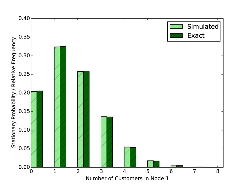
(a) Marginal Distribution of Node 1

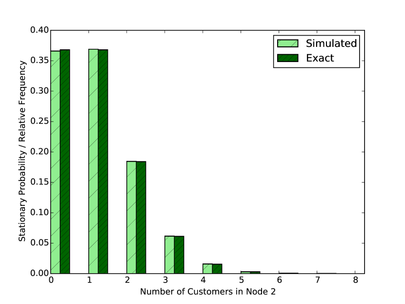
(b) Marginal Distribution of Node 2

Figure 2: A comparison of the simulated marginal distributions and the exact marginals at each node. We see that the exact result from Theorem 3 agrees with the simulation.

Theorem 3 also says that the distribution is the product of the marginals. Let $\hat{\pi}(x_{1},x_{2})$ be the empirical probability of having $x_{1}$ customers at node 1 and $x_{2}$ customers at node 2. Let $\hat{\pi}_{1}(x_{1})$ be the empirical probability of having $x_{1}$ customers at node 1. Let $\hat{\pi}_{2}(x_{2})$ be the empirical probability of having $x_{2}$ customers at node 1. Note that $\hat{\pi}_{1}(\cdot)$ and $\hat{\pi}_{2}(\cdot)$ are shown in Figure 2 and they agree with the result from Theorem 3. In our simulation

$$\sup_{(x_{1},x_{2})\in\mathbb{Z}_{+}^{2}}\left|\hat{\pi}(x_{1},x_{2})-\hat{\pi}_{1}(x_{1})\hat{\pi}_{2}(x_{2})\right|=0.00219$$

when rounded to three significant figures. This shows that the empirical equilibrium distribution of the network is (approximately) a product form distribution. This agrees with the product-form result from Theorem 3.

V Conclusions and Future Work

Motivated by timeouts in Internet services, we have formulated a model for infinite server queueing networks in which routing decisions are based on service time deadlines. In spite of the fact that the usual theory does not apply, we have shown that the model does indeed have a product-form stationary distribution. In addition to providing an analytic proof, we have also provided a simulation which verifies the results.

We have already noted that our proof is heavily dependent on the fact that each node in the network has an infinite number of servers. As a result, our analysis will not immediately transfer to more general networks in which the nodes have finitely many servers. However, our analysis does extend to the case in which only a portion of the overall network has infinite server queues with deadline based routing. We may also be able to extend our analysis to the case of closed networks of infinite server queues.

A less straightforward and more mathematically demanding extension of these results would be to the case of more general arrival processes. Nonstationary Poisson arrivals to infinite server queueing networks were considered in [15] with the main result being that product-form results still hold but are time-varying. Given these previous results, this seems like a fruitful direction for future work.

Finally, we note that deadlines are essential to many applications besides Internet services such as wireless communication [16, 17], patient scheduling [18], low latency computing [19, 20], and utility computing [21, 22, 23]. Consequently, we feel that we may be able to apply similar modeling ideas to other application domains.

References

- [1] B. Urgaonkar, G. Pacifici, P. Shenoy, M. Spreitzer, and A. Tantawi, “An analytical model for multi-tier internet services and its applications,” in ACM SIGMETRICS Performance Evaluation Review, vol. 33, pp. 291–302, ACM, 2005.
- [2] E. G. Coffman, Jr, T. Kadota, and L. A. Shepp, “A stochastic model of fragmentation in dynamic storage allocation,” SIAM Journal on Computing, vol. 14, no. 2, pp. 416–425, 1985.
- [3] T. Dohi, T. Matsuoka, and S. Osaki, “An infinite server queuing model for assessment of the software reliability,” Electronics and Communications in Japan (Part III: Fundamental Electronic Science), vol. 85, no. 3, pp. 43–51, 2002.
- [4] W. Whitt, “Dynamic staffing in a telephone call center aiming to immediately answer all calls,” Operations Research Letters, vol. 24, no. 5, pp. 205–212, 1999.
- [5] Q. Zhang, L. Cheng, and R. Boutaba, “Cloud computing: state-of-the-art and research challenges,” Journal of internet services and applications, vol. 1, no. 1, pp. 7–18, 2010.
- [6] J. R. Jackson, “Jobshop-like queueing systems,” Management science, vol. 10, no. 1, pp. 131–142, 1963.
- [7] F. Baskett, K. M. Chandy, R. R. Muntz, and F. G. Palacios, “Open, closed, and mixed networks of queues with different classes of customers,” Journal of the ACM (JACM), vol. 22, no. 2, pp. 248–260, 1975.
- [8] F. P. Kelly, Reversibility and stochastic networks. Cambridge University Press, 1979.
- [9] H. Chen and D. D. Yao, Fundamentals of queueing networks: Performance, asymptotics, and optimization, vol. 46. Springer Science & Business Media, 2013.
- [10] J. Walrand, An introduction to queueing networks. Prentice Hall, 1988.
- [11] A. Russo and A. Sabelfeld, “Securing timeout instructions in web applications,” in Computer Security Foundations Symposium, 2009. CSF’09. 22nd IEEE, pp. 92–106, IEEE, 2009.
- [12] A. Goldfarb and C. Tucker, “Online display advertising: Targeting and obtrusiveness,” Marketing Science, vol. 30, no. 3, pp. 389–404, 2011.
- [13] A. B. Downey, “Evidence for long-tailed distributions in the internet,” in Proceedings of the 1st ACM SIGCOMM Workshop on Internet Measurement, pp. 229–241, ACM, 2001.
- [14] R. W. Wolff, “Poisson arrivals see time averages,” Operations Research, vol. 30, no. 2, pp. 223–231, 1982.
- [15] W. A. Massey and W. Whitt, “Networks of infinite-server queues with nonstationary poisson input,” Queueing Systems, vol. 13, no. 1-3, pp. 183–250, 1993.
- [16] N. Master and N. Bambos, “Power control for wireless streaming with HOL packet deadlines,” in 2014 IEEE International Conference on Communications (ICC), pp. 2263–2269, IEEE, 2014.
- [17] N. Master and N. Bambos, “Service rate control for jobs with decaying value,” in 2015 American Control Conference (ACC), pp. 3255–3260, IEEE, 2015.
- [18] N. Master, C. W. Chan, and N. Bambos, “Myopic policies for non-preemptive scheduling of jobs with decaying value,” arXiv preprint arXiv:1606.04136, 2016.
- [19] N. Master and N. Bambos, “Low latency policy iteration via parallel processing and randomization,” in 2015 54th IEEE Conference on Decision and Control (CDC), pp. 1084–1091, IEEE, 2015.
- [20] N. Master and N. Bambos, “Randomized iterations for low latency fixed point computation,” in 53rd IEEE Conference on Decision and Control, pp. 5208–5215, IEEE, 2014.
- [21] Z. Zhou and N. Bambos, “A general model for resource allocation in utility computing,” in 2015 American Control Conference (ACC), pp. 1746–1751, IEEE, 2015.
- [22] Z. Zhou, B. Yolken, R. A. Miura-Ko, and N. Bambos, “A game-theoretical formulation of influence networks,” in 2016 American Control Conference (ACC), pp. 3802–3807, IEEE, 2016.
- [23] Z. Zhou and N. Bambos, “Target-rate driven resource sharing in queueing systems,” in 2015 54th IEEE Conference on Decision and Control (CDC), pp. 4940–4945, IEEE, 2015.