Additional energy-information relations in thermodynamics of small systems

Abstract

The Clausius inequality (CI) form of the second law of thermodynamics relates information changes (entropy) to changes in the first moment of the energy (heat and indirectly also work). Are there similar relations between other moments of the energy distribution, and other information measures, or is the Clausius inequality a one of a kind instance of the energy-information paradigm? If there are additional relations, can they be used to make predictions on measurable quantities? Changes in the energy distribution beyond the first moment (average heat or work) are especially important in small systems which are often very far from thermal equilibrium. The generalized Clausius inequalities (GCI’s), here derived, provide positive answers to the two questions above and add another layer to the fundamental connection between energy and information. To illustrate the utility of the new GCI’s, we find scenarios where the GCI’s yield tighter constraints on performance (e.g. in thermal machines) compared to the second law. To obtain the GCI’s we use the Bregman divergence - a mathematical tool found to be highly suitable for energy-information studies. The quantum version of the GCI’s provides a thermodynamic meaning to various quantum coherence measures. It is intriguing to fully map the regime of validity of the GCI’s and extend the present results to more general scenarios including continuous systems and particles exchange with the baths.

I Introduction

Thermodynamics is a remarkable theory. It was originally conceived to describe practical limitations of steam engines, and now it is one of the pillars of theoretical physics with applications in countless systems and scenarios. As Einstein said “It is the only physical theory of universal content, which I am convinced, that within the framework of applicability of its basic concepts will never be overthrown”. It is now established that basic thermodynamic laws such as the Clausius inequality (second law) hold even when the system is composed of a single particle with only few energy levels and the evolution is non classical Alicki (1979); Sagawa (2012); Peres (2006); Esposito and Van den Broeck (2011). Consequently, the Carnot efficiency limit holds for arbitrary small and/or quantum heat machines. Nevertheless, this does not exclude the appearance of quantum effects in microscopic heat machines Uzdin et al. (2015); Gelbwaser-Klimovsky and Kurizki (2014); Mitchison et al. (2015). Even without quantum interference or entanglement the thermodynamics of small systems is fascinating. Small systems like biological machines typically operate far from equilibrium and may be subjected to strong thermal fluctuations. For example, thermodynamics has been applied to the study of biological replication of DNA Andrieux and Gaspard (2008); Jarzynski (2008). More generally, non-equilibrium statistical mechanics, and stochastic thermodynamics have been the subject of intensively study in recent years (see Seifert (2012); Harris and Schütz (2007); Jarzynski (2011) and references therein). A single ion heat engine Roßnagel et al. (2016) and a multiple ion refrigerator Maslennikov et al. (2017) have recently been experimentally demonstrated, and there are various suggestions for heat machine realization in superconducting circuits Niskanen et al. (2007); Campisi et al. (2015), optomechanics Gelbwaser-Klimovsky and Kurizki (2015); Zhang et al. (2014) and cavity QED Mitchison et al. (2016).

Thermodynamics has been traditionally applied to macroscopic objects where deviations from averaged quantities (even outside equilibrium) are too small to be measured or to be of any practical interest. With the growing experimental capabilities in the microscopic realm, there is a growing motivation to consider fluctuations from a thermodynamic point of view and go beyond the first moment of the energy distribution. Are there second laws for other quantities? If there are such laws, we ask if they can be expressed in energy-information form and maintain the structure of the standard second law.

The relation between energy and information has led to a deep understanding of the foundations of thermodynamics. Just to mention a few examples: Maxwell demon, Szilard engine and Landauer erasure principle. The Clausius inequality (CI) presents the energy information relationship in a clear and concise way

$$\Delta S-\int\delta Q/T(t)\geq 0,$$ (1)

$Q$ is the heat exchanged with a bath at temperature $T(t)$, and $S$ is the entropy of the system. The heat and entropy relation is used daily in the study of thermal interactions. For example, in a first order phase transition the latent heat is associated with the disorder difference of the two phases. The Clausius inequality (1) is one of the most versatile forms of the second law. It applies to non-periodic processes, to multiple heat baths (as needed for heat machines), and also for states that are initially and/or finally far from thermal equilibrium Jarzynski (1999). Moreover, as mentioned above, the CI holds even in the quantum microscopic realm.

In contrast to a macroscopic fluid at equilibrium, at the microscopic scale the system typically does not have a classical equation of state with just a few thermodynamic variables. The entropy that appears in the CI in such a case is the von Neumann entropy Peres (2006) of the system, and it is defined regardless of equilibrium or an equation of state. Up to Sec. IV, we deal only with statistical mixtures of energy eigenstates, so the von Neumann entropy reduces to the Shannon entropy in the energy basis of the system $S=\sum_{j}-p_{j}\ln p_{j}$, as in the framework of stochastic thermodynamics Seifert (2012).

In recent years, the second law has been explored and extended in two very different frameworks. The first is stochastic thermodynamics (and non-equilibrium statistical mechanics). The Jarzynski fluctuation relations for work Quan and Dong (2008); Jarzynski (2011), can be viewed as a generalization of the second law (in certain scenarios) which is applicable to higher energy moments. This approach has been successfully applied to heat machines as well Campisi (2014); Campisi et al. (2015). The results in Campisi (2014); Campisi et al. (2015) are important and interesting, but they do not relate changes in information to changes in energy. The other framework that can be viewed as an extension of the second law is thermodynamic resource theory Goold et al. (2016); Horodecki and Oppenheim (2013); Gour et al. (2015); Lostaglio et al. (2015a). In this framework properties of completely positive maps are used to construct monotones that must decrease under thermal interactions with a single bath. Despite the appealing elegance of this framework it has a major drawback: these monotones are so far not related to observable quantities. Nonetheless, there are interesting insights arising from this framework (e.g. Lostaglio et al. (2015b)). More important for the present work is the fact that resource theory is not formulated in terms of information and energy. A more extensive discussion on resource theory appears in Appendix IV.

In this paper we present a third way of extending the second law. Our approach is based on the energy-information paradigm and has the same logic and underlying structure as the standard second law. Our results clearly show that such additional energy-information relations exist. The results presented here should be further extended and explored. Yet, we emphasize that even this first study provides new predictions and significantly extends our understanding of the interplay between energy, information, and the mathematical framework that connects them. A summary of the three approaches for extending the second law is given in Table 1.

Table 1: Comparison between different frameworks that predict constraints on thermodynamic processes. The standard second law is not just a mathematical constraint, it has an energy-entropy structure. Among the known extensions of the second law only the generalized Clausius inequalities here derived provides new energy-information relations. Other features are compared in the text.

Finally, we wish to give one more motivating arguments for the study of additional second laws. Consider the following scenario: a system with a time-independent Hamiltonian $H$ is connected to a thermal bath and reaches a thermal state with an average energy $\left\langle H\right\rangle_{f}$. The heat in this case is determined by the change in the average energy with respect to the initial state $Q=\left\langle H\right\rangle_{f}-\left\langle H\right\rangle_{0}$. When the initial state is not thermal but satisfies $\left\langle H\right\rangle_{0}=\left\langle H\right\rangle_{f}$ something puzzling takes place from the thermodynamic point of view. It is clear that the bath has changed the energy probability distribution of the system (despite the fact that the average has not changed). We ask: 1) Since the system has changed, the bath must have changed as well, is it possible to thermodynamically quantify the change in the bath when $Q=0$? 2) A change in the energy probability distribution of the system, implies that some of the energy moments have changed as well. Is it possible to formulate a thermodynamic framework for the change in energy moments other than the first? Even though there seems to be no immediate reason to assume there are thermodynamic answers to these questions, this paper provides a possible answer by formulating generalized Clausius inequalities for higher order energy moments.

Changes in the higher moments of the energy are not only important for understanding the system dynamics far from equilibrium. They are also important for understanding the back action on heat reservoirs with finite heat capacity. By studying the changes in higher moments of the bath, it is possible to quantify to what extent the bath has deviated from equilibrium by interacting with the system (when the heat capacity of the bath is not infinite as in the ideal case). For example, for a thermal state in the bath, we expect a certain relation between the first and second moment of the energy. This relation still holds if the bath is heated to a different thermal state. However, if energy entered the bath, but the bath does not relax to equilibrium (e.g. because it is too small), then the thermal relation between the moments will no longer hold. We return to this point later on when discussing the impact on the bath.

The term ’generalized Clausius inequality’ has already appeared in Deffner and Lutz (2010). There, the CI is written using the relative entropy, and a divergence inequality is used to obtain an ’improved CI’. The zero in one of the sides of the CI is replaced by some positive number related to the Bures length. However, the physical quantities and the information measures are still the same as in the standard inequality. In contrast, in this study we generalized the energy-information measures to other quantities.

II Main findings

In this section we present the generalized CI’s in their simplest form and not in their more general form derived in Appendix I. In the main text we deal with cases where only one bath is connected to the system at a given time. However several baths can be connected sequentially in time so that the temperature of the bath is time dependent. That is instead of the notation $\sum\beta_{k}Q_{k}$ in the CI we shall use the notation $\intop\frac{\delta Q}{T(t)}$ for sequential connection to multiple baths at different temperatures. The generalization to simultaneous connection to several baths is discussed in Appendix I.

Let the system be composed of a finite set of states $j=1,..,N$ whose energies are $\{E_{j}\}_{j=1}^{N}$. The probability to be in a state ’$j$’ is $p_{j}$ (to separate the stochastic part of the paper from the quantum part, we use quantum notations only in Sec. IV). The energy probability distribution of a thermal state with inverse temperature $\beta=1/T$ is $p_{\beta,j}=e^{-\beta(E_{j}-F)}$, $F=-\frac{1}{\beta}\ln\sum_{j}e^{-\beta E_{j}}=-\frac{1}{\beta}\ln Z$ is the standard free energy, and $Z$ is the partition function. As in the stochastic thermodynamics framework Seifert (2012) the energy levels can be varied in time, and the system (or parts of it) can interact with thermal baths at different temperatures.

Until Sec. III, our main object of interest is the $F$-shifted $\alpha$ energy moment

$$\mathcal{H}_{\alpha} =\left\langle[H(t)-F(t)]^{\alpha}\right\rangle=\sum_{j}p_{j}[E_{j}(t)-F(t)]^{\alpha},$$ (2)

$$F(t) =T(t)\ln\sum_{j}\exp[-E_{j}(t)/T(t)]$$ (3)

where $\alpha$ is a real and positive number ($\alpha$ is not necessarily an integer). This quantity is an observable that can be evaluated from energy measurements. It contains information on higher moments of the energy distribution. The appearance of the instantaneous free energy $F(t)$ is interesting. First, it makes $H-F$ a positive operator so any $\alpha\geq 0$ power of $H-F$ is well defined. Second, it makes $(H-F)^{\alpha}$ invariant to uniform shifts of all the levels by a constant (in contrast to a regular moment $\left\langle H^{\alpha}\right\rangle$). The variance, for example, is also shift-invariant but the subtraction of the average makes the variance a nonlinear function of $p_{j}$ which significantly complicates the analysis. Nonetheless, in a certain class of cases $\mathcal{H}_{2}$ will be equal to to the energy variance. The appearance of $F(t)$ in (2) follows from the derivation of the GCI as explained below.

Now that we have an energy related quantity, it is possible define its flows in the same way it is done for the average energy (e.g. Anders and Giovannetti (2013))

$$\mathcal{W}_{\alpha} \triangleq \int_{t_{i}}^{t_{f}}dt\sum_{j}p_{j}\frac{d}{dt}[(E_{j}-F)^{\alpha}],$$ (4)

$$\mathcal{Q}_{\alpha} \triangleq \int_{t_{i}}^{t_{f}}dt\sum_{j}\frac{dp_{j}}{dt}(E_{j}-F)^{\alpha}.$$ (5)

In the present paper subscript ${}^{\prime}f^{\prime}$ stands for ’final’ and ${}^{\prime}i^{\prime}$ stands for ’initial’ (to prevent confusion ’$i$’ will not be used as a summation index). Just like in the $\alpha=1$ case, the logic behind these definitions is that if the levels are fixed in time, the changes in energy must be due to heat exchange with the environment. If the populations are fixed the change in energy must be work related. From (4) and (5) we get

$$\Delta\mathcal{H}_{\alpha}=\mathcal{Q}_{\alpha}+\mathcal{W}_{\alpha}.$$ (6)

We first consider two elementary thermodynamic primitives: 1) Isochores: the system is coupled to a bath and the energy levels $E_{j}$ do not change in time. 2) Adiabats: the system is not connected to a bath, and the energy levels change in time (energy populations are fixed in time). Note that adiabats need not be slow. The use of this term refers to an ’adiabatic’ process in macroscopic classical thermodynamics, where the system is isolated from the environment, and consequently the entropy of the system does not change in time. Isochores involve only heat, while adiabats involve only work. Other processes such as isotherms can be constructed by concatenating these two primitives Anders and Giovannetti (2013). We now proceed to the derivation of an important family of the GCI the $\alpha$CI.

Let us first consider a basic isochore thermalization process: the system is connected to a single bath with inverse temperature $\beta$ and the levels of the system do not change in time. In Appendix I we show that for isochores

$$\Delta\mathcal{S}_{\alpha}-\frac{\mathcal{Q}_{\alpha}}{T^{\alpha}}=D_{\alpha}^{B}(\vec{p}_{i},\vec{p}_{\beta})-D_{\alpha}^{B}(\vec{p}_{f},\vec{p}_{\beta}).$$ (7)

On the left hand side (LHS) we introduce the $\alpha$ information function $\mathcal{S}_{\alpha}$ which is defined as

$$\mathcal{S}_{\alpha} = \sum_{j}\intop_{c_{0}}^{p_{j}}(-\ln x)^{\alpha}dx=[\sum_{j}\Gamma(\alpha+1,-\ln p_{j})]$$

$$-\Gamma(\alpha+1,0)$$ (8)

Where $\Gamma$ is the indefinite Gamma function. The lower limit of the integral adds a constant term to $\mathcal{S}_{\alpha}$. For convenience, $c_{0}$ was chosen so that $\mathcal{S}_{\alpha}=0$ for deterministic states (one probability is equal to one and the rest are equal to zero). $\mathcal{S}_{1}$ is the standard Shannon entropy $S=-\sum p_{j}\ln p_{j}$. In Appendix V we comment on the physicality of $\mathcal{S}_{\alpha}$ compared to the standard Shannon entropy. In short, we argue that at least in our context $\mathcal{S}_{\alpha}$ and $S$ have the same functionality: both are used to put restrictions on energy changes created by a thermal bath. The relation of $\mathcal{S}_{\alpha}$ to information is discussed after stating the GCI.

On the right hand side (RHS) of (7) we have the Bregman divergence of the initial state of the system $\vec{p}_{i}$ and the final state of the system $\vec{p}_{f}$ with respect to the thermal state $\vec{p}_{\beta}$. The definition of the Bregman divergence $D_{\alpha}^{B}(\vec{p}_{2},\vec{p}_{1})$ is Bregman (1967)

$$D_{\alpha}^{B}(\vec{p}_{2},\vec{p}_{1})\doteq\mathcal{S}_{\alpha}(\vec{p}_{1})-\mathcal{S}_{\alpha}(\vec{p}_{2})+(\vec{p}_{2}-\vec{p}_{1})\cdot\nabla\mathcal{S}_{\alpha}(p_{1})$$ (9)

This divergence and its appealing geometric interpretation are described in Appendix I. For now, it suffices to know only several of its key features. First, mathematically, it is a divergence so it satisfies $D_{\alpha}^{B}(\vec{p}_{2},\vec{p}_{1})\geq 0$ and $D_{\alpha}^{B}(\vec{p}_{2},\vec{p}_{1})=0\>\Leftrightarrow\vec{p}_{2}=\vec{p}_{1}$. Second, $D_{\alpha}^{B}(\vec{p}_{2},\vec{p}_{1})$ is convex in the first argument $\vec{p}_{2}$ (see Appendix I). Third, for $\alpha=1$, $D_{1}^{B}$ is the Kullback-Leibler Divergence (relative entropy) $D_{KL}(\vec{p}_{2},\vec{p}_{1})=\sum_{j}p_{2,j}\ln(p_{2,j}/p_{1,j})$.

Equation (7) is an identity valid for isochore. To make use of it we need to make some physical statements on one of the sides of side of the identity. A thermal interaction is a map $\mathcal{M}_{\beta}(\vec{p}_{i})=\vec{p}_{f}$ with the thermal state as a fixed point $\mathcal{M}_{\beta}(\vec{p}_{\beta})=\vec{p}_{\beta}$. The RHS of (7) is a measure of contractiveness of the map. $D_{\alpha}^{B}(\vec{p},\vec{p}_{\beta})$ can be regarded as a proximity measure (a divergence, not necessarily a distance) between the state $\vec{p}$ and $\vec{p}_{\beta}$. Thus, a positive value in the RHS of (7) implies $\mathcal{M}_{\beta}$ is contractive with respect to $\vec{p}$ (under the $D_{\alpha}^{B}$ measure), i.e. $\vec{p}_{f}$ is closer than $\vec{p}_{i}$ to the fixed point $\vec{p}_{\beta}$ (in terms of $D_{\alpha}^{B}$).

While the LHS is the content of the physical law, the RHS sets its regime of validity. Consider the case of full thermalization where $\vec{p}_{f}=\vec{p}_{\beta}$. Since $D_{\alpha}^{B}(\vec{p}_{f}=\vec{p}_{\beta},\vec{p}_{\beta})=0$ it follows from (7) that $\Delta\mathcal{S}_{\alpha}-\frac{\mathcal{Q}_{\alpha}}{T^{\alpha}}\geq 0$. In Sec. II.5 we show that in addition to the contractiveness interpretation of the RHS, it also has an appealing thermodynamic interpretation related to reversible processes and maximal work extraction.

In Sec. II.3 we discuss cases where the RHS of (7) is guaranteed to be positive, but for now let us assume it is positive for isochores and see how various thermodynamic results emerge. Consider a thermodynamic protocol composed of an infinitesimal concatenation of isochores and adiabats. It is assumed that the isochores are short enough so that the temperature of the bath in each isochore is fixed. Hence, isochore ${}^{\prime}l^{\prime}$ satisfies $\delta\mathcal{S}_{\alpha}^{(l)}-\frac{1}{T_{(l)}{}^{\alpha}}\mathcal{\delta Q}_{\alpha}^{(l)}\geq 0$. The adiabats that connect the isochores carry zero $\alpha$ heat $\delta\mathcal{Q}_{\alpha}=0$ and they do not change the entropy $\delta\mathcal{S}_{\alpha}=0$. Summing the infinitesimal contributions of both isochores and adiabats we get our first main finding: the $\alpha$CI family of the GCI’s

$$\Delta\mathcal{S}_{\alpha}-\int\frac{\frac{d}{dt}\mathcal{Q}_{\alpha}}{T(t)^{\alpha}}dt\geq 0$$ (10)

See (53) for a more general form with simultaneous connection to multiple baths. In the study of heat machines the periodic form of the second law $-\oint\frac{\mathcal{\delta Q}(t)}{T(t)}\geq 0$ is highly useful. For a periodic protocol, as in heat engines and refrigerators, the system reaches a cyclic operation $\vec{p}(t+\tau_{cyc})=\vec{p}(t)$ where $\tau_{cyc}$ is the cycle time. Since in this case $\Delta\mathcal{S}_{\alpha}=\mathcal{S}_{\alpha}[\vec{p}(t+\tau_{cyc})]-\mathcal{S}_{\alpha}[\vec{p}(t)]=0$ we get the analogue of the periodic CI

$$-\oint\frac{\mathcal{\delta Q}_{\alpha}(t)}{T^{\alpha}(t)}\geq 0$$ (11)

where $\delta\mathcal{Q}_{\alpha}$ is the $\alpha$ heat transferred during a short time $dt$. The advantage of this form is that it is completely free of $\mathcal{S}_{\alpha}$.

In isotherms (IST), the system is always in the Gibbs state $p_{\beta}=p_{\beta(t)}[H(t)]=e^{-\beta(t)[H(t)-F(t)]}$ even though $\beta$ and/or the energy levels can vary in time). As shown in the end of Appendix I, by considering an infinitesimal concatenation of isochores and adiabats one can show that

$$\Delta\mathcal{S}_{\alpha}^{IST}-\int\delta\mathcal{Q}_{\alpha}^{IST}/T(t)^{\alpha}=0$$ (12)

There is an alternative and simple way to obtain relation (12) for isotherms. Consider a protocol where the system Hamiltonian is changed in time $H=H(t)$, but the system is always in thermal equilibrium $p_{\beta(t)}(H(t))=e^{-\beta(t)[H(t)-F(t)]}$ (for this the change in H(t) should be much slower than the thermalization time). Using (5) and (8) for isotherms $p=p_{\beta}(t)$ we find

$$\intop\frac{\delta\mathcal{Q}_{\alpha}^{IST}}{T(t)^{\alpha}} =\sum_{j}\intop_{p_{i}}^{p_{fin}}\frac{(H-F)_{j}^{\alpha}}{T(t)^{\alpha}}dp_{,j}$$

$$=\sum_{j}\intop_{p_{i}}^{p_{fin}}(-\ln p_{\beta,j})^{\alpha}dp_{\beta,j}$$

$$\equiv S_{\alpha}(\vec{p}_{\beta,fin})-S_{\alpha}(\vec{p}_{\beta,i})$$ (13)

Therefore we obtain the equality of the GCI $\Delta\mathcal{S}_{\alpha}^{IST}=\intop\beta(t)^{\alpha}\delta\mathcal{Q}_{\alpha}^{IST}$.

Reversible processes consist of (non-infinitesimal) sequences of isotherms and adiabats (for adiabats $\Delta\mathcal{S}_{\alpha}=\mathcal{Q}_{\alpha}=0$) so we can write

$$\Delta\mathcal{S}_{\alpha}-\int\frac{\delta\mathcal{Q}_{\alpha}^{R}}{T(t)^{\alpha}}=0.$$ (14)

where $\mathcal{Q}_{\alpha}^{R}$ is the heat absorbed in a reversible process. We now wish to clarify the difference between (12) and (14). Any isotherm must start and end in thermal equilibrium. Thus, the endpoints of adiabats between isotherms are fully determined. However, an adiabat at the end of the protocol need not end at a thermal state. Consequently, a reversible process may involve a final state that is very different from a thermal state (a similar argument can be applied for the initial state). Nonetheless, (14) states that the equality in the GCI is valid also for reversible processes that start or end out of equilibrium.

Finally, we conclude that the GCI’s are not just inequalities; they are inequalities that are saturated for reversible processes. In perfect analogy to the standard second law, if a reversible process is given the CI implies that all possible irreversible process with the same endpoint, will be less optimal (e.g. produce less work and consume more heat). This is discussed in detail in Sec. II.2.

II.1 Information in the GCI and extensivity

By virtue of the GCI $\mathcal{S}_{\alpha}$ is the information conjugated to $\mathcal{Q}{}_{\alpha}$ heat. The reasons for associating $\mathcal{S}_{\alpha}$ with information are the following: 1) $\mathcal{S}_{\alpha}$ of a pure (deterministic) state is zero. 2) $\mathcal{S}_{\alpha}$ is symmetric. It is invariant to rearrangement (permutation) of the probabilities. 3) It increases under doubly stochastic transformations, and it obtains a maximal value for the uniform distribution. The third property follows from the fact that $\mathcal{S}_{\alpha}$ is Schur concave. The Schur concavity is a built-in feature of the Bregman formalism described in Appendix I. The reason for expecting this property is that doubly stochastic transformations are mixtures of permutations, and they smear out the probability distribution and make it more random.

Note that we have not imposed further requirements on the information measure such as extensivity. $\mathcal{Q}{}_{\alpha}$ is in general not an extensive quantity so the information conjugated to it need not be extensive as well.

II.2 Single bath forms and reversible state preparation

In this section we study the case where a single bath with a fixed temperature $T$ is available to interact with the system (in contrast to the more general $T(t)$ used until now). From (10) and (14) we conclude that in the validity regime of the CI, any process that includes adiabats, isotherms, and isochores satisfies

$$\mathcal{Q}_{\alpha} \leq \mathcal{Q}_{\alpha}^{R},$$ (15)

$$\mathcal{W}_{\alpha} \geq \mathcal{W}_{\alpha}^{R},$$ (16)

where $\mathcal{Q}_{\alpha}^{R},\mathcal{W}_{\alpha}^{R}$ are the $\alpha$ reversible heat, and $\alpha$ reversible work gained by going from $\{\vec{p}_{i},H_{i}\}$ to $\{\vec{p}_{f},H_{f}\}$ in a reversible protocol. $\mathcal{Q}_{\alpha},\mathcal{W}_{\alpha}$ are the heat and work gained in an irreversible process between the same $\{\vec{p},H\}$ endpoints. Equation (16) is obtained from (15) and (6).

In analogy to standard thermodynamics, the reversible $\alpha$ work that can be extracted by going from $\{\vec{p}_{i},H_{i}\}$ to $\{\vec{p}_{f},H_{f}\}$, takes the form

$$\mathcal{W}^{R} = \Delta\mathcal{F}_{\alpha}-T^{\alpha}D_{\alpha}^{B}(\vec{p}_{i},\vec{p}_{\beta,i})+T^{\alpha}D_{\alpha}^{B}(\vec{p}_{f},\vec{p}_{\beta,f}),$$

$$\vec{p}_{\beta,i(f)} = exp[-\beta(H_{i(f)}-F_{i(f)})],$$ (18)

where $\mathcal{F}_{\alpha}=\mathcal{H}_{\alpha}(\vec{p}_{\beta})-T^{\alpha}\mathcal{S}_{\alpha}(\vec{p}_{\beta})$ is the $\alpha$ order (equilibrium) free energy. Equation (LABEL:eq:_WR_berg) is proven in Appendix II. Note that one can also define a quantity $\tilde{\mathcal{F}}_{\alpha}(\vec{p})=\mathcal{H_{\alpha}}(\vec{p})-T^{\alpha}\mathcal{S}_{\alpha}(\vec{p})$ that is the $\alpha$CI analogue of the non-equilibrium free energy Still et al. (2012); Esposito and Van den Broeck (2011) (for equilibrium states $\tilde{\mathcal{F}}_{\alpha}(\vec{p}_{\beta})=\mathcal{F}_{\alpha}$). With this definition the $\mathcal{W}_{\alpha}^{R}$ is given by $\mathcal{W}_{\alpha}^{R}=\Delta\tilde{\mathcal{F}}_{\alpha}$.

We point out that Landauer erasure Reeb and Wolf (2014) is a special case of thermal state preparation. Thus, the reversible limit (15)-(LABEL:eq:_WR_berg) bounds the changes in $\alpha$ moments in erasure scenarios as well.

From (15) and (16), we deduct the single bath cyclic formulation of the second law $\oint d\mathcal{W}_{\alpha}\geq 0$ : it is impossible to extract $\alpha$ work in a periodic process with a single bath. Similarly, $\oint d\mathcal{Q}_{\alpha}\leq 0$ implies that an $\alpha$ heat cannot be extracted from a single bath in a periodic process (the changes in the bath are studied in Appendix III).

II.3 Regime of validity

From (7) the $\alpha$CI’s (10) validity condition for a single bath isochore is

$$D_{\alpha}^{B}(\vec{p}_{i},\vec{p}_{\beta})-D_{\alpha}^{B}(\vec{p}_{f},\vec{p}_{\beta})\geq 0.$$ (19)

Next, it is shown that this validity condition is guaranteed to hold in the following cases:

• Strong thermalization: $\vec{p}_{f}$ is equal or sufficiently close to $\vec{p}_{\beta}$.

• Uniform thermalization map $\vec{p}_{f}=(1-y)\vec{p}_{i}+y\vec{p}_{\beta}$ where $0\leq y\leq 1$.

• Two-level system

• Isotherms

• Adiabats

The first regime follows from the fact that $D_{\alpha}^{B}(\vec{p}_{f}\to\vec{p}_{\beta},\vec{p}_{\beta})\to 0$ so that the RHS of (7) is positive. This is a very important regime as it can take place in different thermalization mechanisms and also in the presence of initial correlation with the bath. Usually for the $\alpha=1$ CI it is assumed that the system and bath Sagawa (2012); Peres (2006) are initially uncorrelated. However, this is not a necessary condition when the final state is thermal or very close to it. Thus, the first validity regime is indifferent to initial system-bath correlations for any $\alpha>0$.

The second regime follows from the fact that the Bregman divergence (9) is convex in its first argument . The third regime holds since the thermalization of a two-level system is always uniform so the two-level case is always contained in the second regime. For isotherms each of the divergence terms in (19) is zero so the $\alpha$CI holds as an equality. For adiabats $\vec{p}_{f}=\vec{p}_{i}$, and once again we get zeros in (19).

Potentially, the regime of validity is much larger than outlined above. Numerical studies showed that significant deviations from the uniform thermalization map still satisfy (19). This is a subject for further research. Nevertheless, the examples given later demonstrate that the above regimes are already sufficient for showing that the various $\alpha$CI bring new insights to thermodynamic scenarios of microscopic systems.

For $\alpha=1$, the $\alpha$CI reduce to the CI and the $D^{B}$ in the validity condition in (19) reduces to the relative entropy. When the thermalization can be described by a completely positive trace preserving map (CPTP) with a Gibbs state as a fixed point, the relative entropy of a state with respect to a fixed point of the map is always decreasing (including quantum dynamics). This means that condition (19) for $\alpha=1$ is satisfied for such thermalization maps. CPTP maps arise naturally when an initially uncorrelated system and a bath interact via a unitary operation. The thermal operations in thermodynamic resource theory are an example of such operations. From this we conclude that for $\alpha=1$ our derivation has the same validity regime as that obtained from other derivations based on CPTP maps Peres (2006); Sagawa (2012); Esposito and Van den Broeck (2011); Spohn (1978); H.-P. Breuer and F. Petruccione (2002); Alicki (1979).

For $\alpha\neq 1$ condition (19) may not be satisfied for CPTP. For example, consider a three-level system where all levels are initially populated. If only levels two and three are coupled to a bath then in general (19) may not hold for $\alpha\neq 1$ (even though the ratio of $p_{3}/p_{2}$ gets closer to the Gibbs factor $exp[-\beta(E_{3}-E_{2})]$).

A smaller regime of validity is not always a disadvantage. The invalidity of one of the $\alpha$CI can give us information on the thermalization process under progress. For example, if in a periodic system (11) is not satisfied we can rule out any of the thermalization scenarios described in the bullets above. Moreover, a regime of invalidity might be useful for some purposes since it is less constrained. Applying such ideas for $\alpha\neq 1$ in heat machines is outside the scope of this paper.

II.4 Allowed operations

Analogously to thermodynamic resource theory Goold et al. (2016); Horodecki and Oppenheim (2013); Gour et al. (2015), the regime of validity can be formulated in terms of allowed operations. Instead of giving a validity condition it is possible to restrict the set of allowed physical processes. Assuming that the system starts in valid initial condition, any allowed operation will keep the system in the validity regime. For example, in a restricted set of operations that includes only full thermalization, uniform thermalization, and adiabats, the generalized Clausius inequalities hold.

II.5 Functional definition of a bath and reversible work availability

Equation (7) is the quintessence of the second law (CI more accurately): both the standard CI and the generalizations that are considered here. Thermodynamics describes interactions with baths. What is a bath, then? There are two main answers and both are useful. One approach describes the bath and its physical properties such as temperature, correlation function, heat capacity etc. As a second approach we suggest the functional definition of a bath. The ideal operation of a bath would be to take any initial state of a system and change some of its properties (e.g. energy moments, or other observables) into predefined values that are independent of the initial state. For example, a thermal bath takes any initial state to a Gibbs state $\vec{p}_{\beta}$ with temperature $1/\beta$. The Gibbs state is the fixed point of the map the bath induces on the system.

In practice the bath is not connected to the system for an infinite amount of time so the process may not be completed. Moreover, if the bath is small compared to the system, it may not have enough energy to complete the thermalization of the system (even though the Gibbs state is a fixed point of this interaction). Nonetheless, it is expected that the final state in these scenarios will be “closer” to the thermal state compared to the initial state. What is the measure of proximity we should use in order to make sure we have valid thermodynamic laws e.g. (10)? This is exactly the Bregman divergence difference (19).

Equation (7) tells us that if the RHS is negative it simply indicates that the device we used for a bath has failed to operate as a bath since it did not decrease the proximity measure of interest.

A “good bath” is one that satisfies (19) for any $\vec{p}_{i}$, however for specific applications such as heat machines it may be sufficient that this condition holds only for the $\vec{p}_{i}$ and $\vec{p}_{f}$ of interest (e.g. those that appear in cyclic operation).

Condition (19) has a very appealing thermodynamic interpretation. From (16) and (LABEL:eq:_WR_berg) we see that $T^{\alpha}D_{\alpha}^{B}(\vec{p}_{i},\vec{p}_{\beta})$ expresses the maximal $\alpha$ work that can be extracted by going from $\vec{p}_{i}$ to $\vec{p}_{\beta}$ when the initial Hamiltonian and final Hamiltonian are equal (but may be changed in the middle) so that $\Delta\mathcal{F}_{\alpha}=0$. Let us use the term “available $\alpha$ work” $\mathcal{A}_{\alpha}(\vec{p}_{i})\triangleq T^{\alpha}D_{\alpha}^{B}(\vec{p}_{i},\vec{p}_{\beta})$. The quantity $\mathcal{A}_{\alpha}$ is analogous to the ergotropy A. E. Allahverdyan, R. Balian, and Th. M. Nieuwenhuizen (2004) in closed quantum systems. The only difference is that ergotropy quantifies the work that can be extracted using only unitaries, while here a bath can be connected as well.

In general, when thermalizing we expect that $\mathcal{A}_{\alpha}$ will decrease. This means that the thermal bath makes the system less “thermally active”. In full thermalization the state becomes $\vec{p}_{\beta}$ which is “thermally passive” ($\mathcal{A}_{\alpha}=0$).

II.6 Intermediate summary

The underlying principles of the thermodynamic generalized Clausius inequalities as studied so far in this paper can be summarized as follows:

• Changes in $\alpha$ order energy moments are associated with changes in a corresponding information measure $\mathcal{S}_{\alpha}$. The two are related by $\alpha$ order Clausius inequality (10) and (53). The GCI’s establish new energy-information relations.

• The generalized Clausius inequalities saturate and become equalities in reversible thermodynamic processes.

• Different energy moments are associated with different divergences that constitute a validity criterion for the functionality of the bath. When the bath brings the system closer to the thermal state according to the $\alpha$ divergence measure, the generalized $\alpha$ order Clausius inequality holds.

• Several important $\alpha$CI validity regimes have been identified but it is important to explore and find additional regimes.

III Additional second laws based on Rényi entropy and $\alpha$ impurity

In the $\alpha$CI we started with some energy moments of interest (2) and found the corresponding information measure that is related to it via the $\alpha$CI. In this section we go in the other direction: we pick information quantities of interest and find the moments that are related to them via the GCI.

As shown in Appendix I, $\partial_{p}\mathcal{S}(p)$ can be any monotonically decreasing function in $p\in[0,1]$, and lead to a generalized Clausius inequality. Alternatively, $\mathcal{S}$ can be any concave and differentiable function in the regime $p\in[0,1]$. Let us first choose $\mathcal{S}$ to be the $\tilde{\alpha}$ impurity Havrda and Charvát (1967); Vajda (1968); Daróczy (1970); Tsallis (1988); Abe and Okamoto (2001) $\mathcal{S}_{\tilde{\alpha}}(\vec{p})=\frac{1}{\tilde{\alpha}-1}(1-\sum p_{j}^{\tilde{\alpha}})$ ($\tilde{\alpha}\geq 0$ can be a fraction). This quantity is often called “Tsallis entropy” Tsallis (1988); Abe and Okamoto (2001), but to prevent unnecessary technical confusions we use here the term “$\tilde{\alpha}$ impurity”. . For $\tilde{\alpha}\geq 0$, $\partial_{p}\mathcal{S}_{\tilde{\alpha}}$ is a decreasing function and we can use our GCI formalism and get the analogue of (7) for the $\alpha$ impurity

$$\Delta\mathcal{S}_{\tilde{\alpha}}^{B}+\frac{\tilde{\alpha}}{\tilde{\alpha}-1}\Delta\left\langle e^{-(\tilde{\alpha}-1)\beta(H-F)}\right\rangle =D_{\tilde{\alpha}}^{B}(\vec{p}_{i},\vec{p}_{\beta})$$

$$-D_{\tilde{\alpha}}^{B}(\vec{p}_{f},\vec{p}_{\beta})$$ (20)

The GCI (20) is written here for simplicity just for isochores. From the time derivative of the observable $+\frac{\tilde{\alpha}}{\tilde{\alpha}-1}\left\langle e^{-(\tilde{\alpha}-1)\beta(H-F)}\right\rangle$ one can define $\tilde{\alpha}$ heat and $\tilde{\alpha}$ work and get an $\tilde{\alpha}$CI valid for isochores, isotherms adiabats, and their combination (as done in Sec. 2)

$$\Delta\mathcal{S}_{\tilde{\alpha}}^{B}-\intop\delta Q_{\tilde{\alpha}} \geq 0,$$ (21)

$$\delta Q_{\tilde{\alpha}} =\frac{\tilde{\alpha}}{\tilde{\alpha}-1}\sum_{j}\delta p_{j}e^{-(\tilde{\alpha}-1)\beta(E_{j}-F)}.$$ (22)

As in the previous generalized CI, when setting $\tilde{\alpha}=1$ in (20) it reduces to the standard Clausius inequality. Another important case is $\tilde{\alpha}=2$ where $\mathcal{S}_{\tilde{\alpha}}^{B}$ is equal to minus the purity of the state (plus a constant), and the Bregman divergence is the standard Euclidean distance squared $D_{\tilde{\alpha}}^{B}(\vec{p}_{i},\vec{p}_{\beta})=\left\|\vec{p}_{i}-\vec{p}_{\beta}\right\|_{2}^{2}$. While in general the Bregman divergence is not a distance, for $\tilde{\alpha}=2$ it is. The regime of validity is given by the positivity of the RHS of (20). The regime of guaranteed validity is at least as large as that given in Sec. II.3. This time the information we obtain is on $\left\langle e^{-(\tilde{\alpha}-1)\beta(H-F)}\right\rangle=\sum p_{j}e^{-(\tilde{\alpha}-1)\beta(E_{j}-F)}$. The information on higher order moments of the distribution is wrapped in an exponential form. In fact, this exponential form is the moment generating function of the distribution. Using the Markov inequality it is possible to learn about the tail of the distribution $P(e^{-(\tilde{\alpha}-1)\beta(E_{j}-F)}\geq\xi)\geq\frac{\left\langle e^{-(\tilde{\alpha}-1)\beta(H-F)}\right\rangle}{\xi}$. Another advantage of this form is that the free energy can easily be pulled out and be replaced by a different constant $E_{ref}$ :

$$\left\langle e^{-(\tilde{\alpha}-1)\beta(H-F)}\right\rangle =$$

$$e^{-(\tilde{\alpha}-1)\beta(E_{ref}-F)}\left\langle e^{-(\tilde{\alpha}-1)\beta(H-E_{ref})}\right\rangle.$$ (23)

For example, $E_{ref}$ can be the ground state energy or the average energy. For $E_{ref}=0$ (23) shows that $F$ is a factor that can be pulled out from the expectation value (in contrast to $\mathcal{H}_{\alpha}$). This is useful when considering the interaction with the bath (see Appendix III).

Here as well, there is a periodic form of the $\tilde{\alpha}$ second law

$$\frac{1}{\tilde{\alpha}-1}\oint_{k}\sum_{j}dp_{j}e^{-(\tilde{\alpha}-1)\beta_{k}(t)[E_{k,j}(t)-F_{k}(t)]}\geq 0$$ (24)

The $\oint_{k}$ symbol stands for summation over connection to different baths $\beta_{k}$ during a cycle.

The GCI can be applied to the Rényi entropy $R_{\bar{\alpha}}(\vec{p})=\frac{1}{1-\bar{\alpha}}\ln\sum p_{j}^{\bar{\alpha}}$ as well. This time $\bar{\alpha}$ is limited to $0\leq\bar{\alpha}\leq 1$ where the Rényi entropy is concave. For $\bar{\alpha}=1$ the Rényi entropy reduces to the Shannon entropy. The $\bar{\alpha}$CI is given by (20) with $\mathcal{S}_{\tilde{\alpha}}^{B}\to R_{\bar{\alpha}}$ and $\delta\mathcal{Q}_{\tilde{\alpha}}\to\delta\mathcal{Q}_{\bar{\alpha}}$

$$\delta Q_{\bar{\alpha}}=\frac{\bar{\alpha}}{1-\bar{\alpha}}\frac{\sum_{j}\delta p_{j}e^{-\beta(\bar{\alpha}-1)(E_{j}-F)}}{\sum_{j}(p_{\beta,j})^{\bar{\alpha}}}.$$ (25)

The validity regime is at least as large as described in Sec. II.3. In the $\bar{\alpha}$CI analogue of (7) the divergence is given by the Bregman divergence with $R_{\bar{\alpha}}$ instead of $\mathcal{S}_{\alpha}$. This divergence is not the Rényi divergence that is used in thermodynamic resource theory Goold et al. (2016); Horodecki and Oppenheim (2013); Gour et al. (2015).

III.1 High temperature limit

In this section we study the high temperature limit of the $\tilde{\alpha}$ impurity GCI ($\tilde{\alpha}$CI). First we consider periodic operation (24) where $\mathcal{S}$ does not appear. For any $\beta$ that is small enough, the Taylor expansion of the exponent in (24) leads to the standard periodic form of the second law $-\oint\frac{dQ}{T}\geq 0$. This is interesting until now we to obtain the CI from a GCI we took the limit $\alpha\to 1,\tilde{\alpha}\to 1,$ etc. However here we see that the periodic form emerges for high temperatures even when $\tilde{\alpha}\neq 1$. To be more precise the condition for being hot enough emerges from the expression.

$$\left\langle e^{-\beta(\tilde{\alpha}-1)(H-F)}\right\rangle =e^{-\beta(\tilde{\alpha}-1)(\frac{E_{max}+E_{min}}{2}-F)}$$

$$\left\langle e^{-\beta(\tilde{\alpha}-1)(H-\frac{E_{max}+E_{min}}{2})}\right\rangle$$ (26)

In order to approximate the exponent in the triangular brackets with a linear term in $H$ the temperature must satisfy the condition

$$T\gg\left|\tilde{\alpha}-1\right|(E_{max}-E_{min})/2.$$ (27)

When this condition holds (24) reduces to the periodic CI $-\oint\frac{\mathcal{\delta Q}(t)}{T(t)}\geq 0$. A more interesting result appears in the non-periodic form of the $\tilde{\alpha}$CI. Using (27) in (21) we get

$$\Delta\mathcal{S}_{\tilde{\alpha}}-\tilde{\alpha}e^{+\beta(\tilde{\alpha}-1)(\frac{E_{max}+E_{min}}{2}-F)}Q/T\geq 0.$$ (28)

Equation (28) implies that on top of the Shannon entropy there are different information measures that put additional constraints on the standard heat exchange with the bath. While (28) offers no advantage for reversible processes, for irreversible processes it can provide a tighter bound on the heat. An example for the superiority of (28) over (1) is given in Sec. V.

This finding paves the way for studying information measures that provide tighter bounds (compared to the second law) on the heat in irreversible processes in various limits (e.g. in cold temperatures). Although we have focused on the $\tilde{\alpha}$ impurity GCI, the high temperature limit can be studied for the Rényi entropy as well.

IV Quantum generalized CI and thermodynamic coherence measures

Let $g(x)$ be an analytic and concave function of $x$. We denote its integral by $G(x)=\intop_{x_{0}}^{x}g(x^{\prime})dx^{\prime}$ where $x_{0}$ will be chosen later. The Bregman matrix divergence Nock et al. (2013); Molnár et al. (2016) is

$$D_{g}^{B}(\rho_{2},\rho_{1}) =\mathcal{S}_{g}(\rho_{1})-\mathcal{S}_{g}(\rho_{2})+tr[(\rho_{2}-\rho_{1})g(\rho_{1})]$$ (29)

$$\mathcal{S}_{g}(\rho_{1}) =tr[G(\rho)]$$ (30)

Repeating the stochastic derivation carried out in Sec. II and in Appendix I, we obtain the quantum generalized CI (QGCI):

$$\Delta\mathcal{S}_{g}-\intop\frac{\delta\mathcal{Q}_{\alpha}}{T^{\alpha}} \geq 0,$$ (31)

$$\delta\mathcal{Q}_{\alpha} =tr[\delta\rho(H-F)^{\alpha}].$$ (32)

We wrote down the quantum form of the stochastic $\alpha$CI (10), but it is equally possible to write the quantum analogue of the other forms (e.g. the Rényi form (25)). To obtain the $\alpha$ form we have set $g(x)=(-\ln x)^{\alpha}$. This time, $\mathcal{S}_{g}$ (30) is defined for density matrices with coherence. $\mathcal{S}_{g}$ has several properties we expect from information measures: 1) it is unitarily invariant (extension of the symmetry property in the stochastic case) 2) it increases under doubly stochastic maps 3) $min(\mathcal{S}_{g})=0$ is obtained for pure states $\left|\psi\right\rangle\left\langle\psi\right|$ ($x_{0}$ can always be chosen so that the minimum of $\mathcal{S}_{g}$ is equal to zero) 4) $\mathcal{S}_{g}$ is maximal for a fully mixed state. 5) $\mathcal{S}_{g}$ increases under any dephasing operation.

The validity regime for the stochastic laws described in Sec. II.3, holds also for the QGCI. Unlike the GCI studied earlier, the adiabats (pure work stage) in the QGCI can include any unitary and not only ones in which the energy levels are modified and the probabilities remain the same. Another important difference with respect to the stochastic GCI arises from the following property of the Bregman matrix divergence. Let $\Lambda$ be a diagonal matrix, and $\rho_{\Lambda}$ be the diagonal part of density matrix $\rho$. The Bregman matrix divergence satisfies

$$D_{g}^{B}(\rho,\Lambda) =D_{g}^{B}(\rho_{\Lambda},\Lambda)+C_{g}(\rho),$$ (33)

where $D_{f}^{B}(\rho_{\Lambda},\Lambda)$ is the vector Bregman divergence (9) of the populations in the $\Lambda$ basis, and the Bregman coherence measure is

$$C_{g}(\rho)=\mathcal{S}_{g}(\rho_{\Lambda})-\mathcal{S}_{g}(\rho)\equiv D_{g}^{B}(\rho,\rho_{\Lambda}).$$ (34)

This coherence measure has the expected basic properties of a coherence measure: 1) It is zero for diagonal states 2) It is maximal for the maximal coherence state $\frac{1}{\sqrt{N}}\sum_{l=1}^{N}\left|l\right\rangle$. 3) It decreases under any dephasing operation. These features follow from the Schur concavity of $\mathcal{S}_{g}(\rho)$.

Before discussing a certain thermodynamic meaning of $C_{g}$ we point out that the contractivity condition for isochores now reads

$$D_{g}^{B}(\rho_{i},\rho_{0})-D_{g}^{B}(\rho_{f},\rho_{0}) =D_{g}^{B}(\vec{p}_{i},\vec{p}_{0})-D_{g}^{B}(\vec{p}_{f},\vec{p}_{0})$$

$$+C_{g}(\rho_{i})-C_{g}(\rho_{f}).$$ (35)

The implication is that even in cases where the stochastic law may not hold (i.e. the first two terms in (35) amount to a negative number), a significant enough coherence erasure $C_{g}(\rho_{i})-C_{g}(\rho_{f})\geq 0$ can be sufficient for making (35) positive. Thus the quantum GCI’s can be valid where the stochastic GCI’s are not.

IV.1 The thermodynamic operational meaning of various coherence measures

In the seminal work Baumgratz et al. (2014) coherence measures were studied from a theoretical point of view without a direct operational meaning. One of these measures is the quantum relative entropy $D(\rho,\rho_{\Lambda})$ (obtained from (29) by choosing $g=-\ln(x)$). In Kammerlander and Anders (2016) it was shown that $D(\rho,\rho_{\Lambda})$ has a clear quantum thermodynamic meaning: $TD(\rho,\rho_{\Lambda})$ is the maximal amount of work that can be extracted from a bath at temperature $T$ using coherence in the energy basis. $\rho$ is the initial state of system, and $\rho_{\Lambda}$ is the final state of the system. In addition, the initial and final Hamiltonian are the same. Since the energy of the system does not change from end to end, the work transferred to the work repository comes from the bath $-W_{max}=Q_{max}=TD(\rho,\rho_{\Lambda})$. Yet, to accommodate the second law, this heat-to-work conversion must come from erasing the coherence. The amount of coherence to be erased is given by the coherence measure $D(\rho,\rho_{\Lambda})$.

In Kammerlander and Anders (2016) an explicit reversible protocol was described to achieve this maximal work extraction limit. The protocol in Kammerlander and Anders (2016) is identical to that described in appendix II with an additional step where transient pulse (work stroke, a unitary) is applied to bring $\rho$ to a diagonal form in the energy basis. Since the only system-bath interaction in the protocol is an isotherm the result $Q_{max}=TD(\rho,\rho_{\Lambda})$ follows directly form the reversible limit of the second law. Repeating the same protocol but with the $\alpha$CI we get:

$$\mathcal{Q}_{\alpha}^{max}=T^{\alpha}D_{\alpha}^{B}(\rho,\rho_{\Lambda}).$$ (36)

Any irreversible protocol that generates $\rho\to\rho_{\Lambda}$ will involve less $\mathcal{Q}_{\alpha}$ flow to the system. A concrete irreversible protocol is given in appendix VI.

In cases where $\mathcal{Q}_{\alpha}$ can be related to the standard heat $\mathcal{Q}_{1}$ (e.g. in two-level systems or when condition (27) holds) the Bregman coherence measure $D_{\alpha}^{B}(\rho,\rho_{\Lambda})$ can produce tighter bounds on the extractable heat and work. For a two-level system and the irreversible protocol described in Appendix VI we have numerically verified that a tighter bound on heat extraction using coherence is obtained compared to the standard second law Kammerlander and Anders (2016).

In Appendix VI, we give an example where coherences are used to extract $Q_{2}$ heat from a thermal bath while exchanging zero standard ($\alpha=1$) heat. This example illustrates the following point. In reversible protocols for any $\alpha$, the $Q_{\alpha}$ are completely determined by the initial state and the temperatures of the bath. In irreversible protocols it is possible to extract different portions of the maximal $Q_{\alpha}$ determined by the GCI. Thus irreversible protocols offer more flexibility in manipulating energy distribution via thermal interaction.

In future studies it is interesting to look for additional quantum features associate with higher moments of the energy.

V Examples and implications

Next, we wish to demonstrate by explicit examples that the GCI’s provide useful information and additional constraints on top of that provided by the standard CI. Finding the highest impact examples is a matter of long term research. Instead, our goal is to show that even in simple scenarios the GCI’s provide important new input.

V.1 High temperature limit

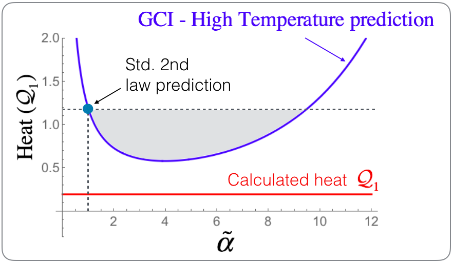
Figure 1: High temperature limit of the $\tilde{\alpha}$ impurity-based GCI, applied to a three-level thermalization process (isochore). For values of $\tilde{\alpha}$ that correspond to the shaded area, the GCI (28) imposes a tighter constraint on the standard $\mathcal{Q}_{1}$ heat compared to the standard second law $\tilde{\alpha}=1$ (dashed-horizontal line).

To illustrate the advantage of (28) over the standard CI we consider an isochore that eventually fully thermalizes the system. The chosen energy levels are $E=\{-\frac{1}{2},0,\frac{1}{2}\}$, the initial state is $p_{0}=\{\frac{1}{2},\frac{1}{2},0\}$, and the temperature is $T=3$. Figure 1 shows that there is a regime of $\tilde{\alpha}$ where the $\tilde{\alpha}$CI provide a tighter bound on the heat. Of course, (28) can be used only when condition (27) holds. As discussed in Sec. III.1 this example motivates the study of new information measures for bounding the heat transfer in irreversible processes. It also illustrates the point that even though the GCI’s typically provide predictions on new quantities such as $\mathcal{Q}_{\alpha}$, in some scenarios we can use the GCI’s to learn on standard quantities such as the standard heat. The GCI’s predictions on the heat can be better than the prediction of the standard CI.

V.2 Zero standard heat thermodynamics

V.2.1 Irreversible case

Let us recall the zero heat scenario described in the introduction, and see what insights the $\alpha$CI can provide. We consider the irreversible case of a simple isochore. Our system has three or more non-degenerate levels. When connected for a long time to a bath with inverse temperature $\beta$ (isochore) the final energy of the system is $\left\langle H\right\rangle_{\beta}=\sum_{j}p_{\beta,j}E_{j}$ regardless of the initial condition ($\vec{p}_{\beta}$ is the thermal Gibbs state). Now we choose an initial condition $\vec{p}_{i}\neq\vec{p}_{\beta}$ that satisfies $\left\langle H\right\rangle_{i}=\sum_{j}p_{i,j}E_{j}=\left\langle H\right\rangle_{\beta}$, and we let the system reach $\vec{p}_{\beta}$ (or close enough to it for all practical purposes). As a result $\left\langle H\right\rangle_{i}=\left\langle H\right\rangle_{f}=\left\langle H\right\rangle_{\beta}$. Since it is an isochore, there is no work in this scenario, and therefore $Q=\Delta\left\langle H\right\rangle-W=\Delta\left\langle H\right\rangle=0$. In this case the standard second law (CI) yields

$$\Delta S\geq 0.$$ (37)

This, however, is a trivial and mathematical statement that can be obtained even without the CI. The thermal state has the maximal amount of entropy for a fixed average energy. Since the input and output state have the same energy, and the output state is thermal, it follows that the entropy of the input state must be lower, and we get $\Delta S\geq 0$. Moreover, one of the key ideas in thermodynamics is the connection between entropy (information) and energy, and the second law provides no such connection in this case.

Now, let us apply the $\alpha$CI. The second order heat is in general non-zero. Even if it is zero in some specific case, there is a higher order heat that is different from zero. For $Q=0$ isochores

$$\mathcal{Q}_{2}=\Delta\left\langle(H-F)^{2}\right\rangle=\Delta\left\langle(H-\left\langle H\right\rangle)^{2}\right\rangle.$$ (38)

Thus, in $Q=0$ isochores, $\mathcal{Q}_{2}$ is the change in the variance of the energy distribution. In contrast to the $\Delta S\geq 0$ for $\alpha=1$ (CI), the $\alpha=2$ GCI, gives us information on the energy variance change

$$\Delta\left\langle(H-\left\langle H\right\rangle)^{2}\right\rangle\leq T^{2}\Delta\mathcal{S}_{2}.$$ (39)

Full thermalization was used for clarity. Equation (39) is equally valid in cases where the initial state undergoes partial thermalization that satisfies $Q=0$. From this example we see that the standard thermodynamic quantities such as the entropy and the average energy are not sufficient for the thermodynamic description of zero heat processes, and other quantities such as $\mathcal{H}_{\alpha}$ and $\mathcal{S}_{\alpha}$ are needed.

It is interesting if in second order phase transitions where the latent heat is zero, there is a non zero $\alpha$ latent heat which is related to changes in $\mathcal{S}_{\alpha}$.

V.2.2 Reversible case

Consider the thermodynamic state preparation scenario where the goal is to transform a state $p_{i}$ to some other state $p_{f}$ (see Sec. II.2 and Appendix II). If the protocol is reversible then according to the standard second law the heat cost is $Q=\mathcal{Q}_{1}=T[S(\vec{p}_{f})-S(\vec{p}_{i})]$ where $S=\mathcal{S}_{1}$ is the Shannon entropy.

In systems with three levels or more, there are different distributions that have the same entropy. In particular, it is possible to have $S(\vec{p}_{f})=S(\vec{p}_{i})$ where $\vec{p}_{f}\neq\vec{p}_{i}$ and $\vec{p}_{f}$ is not a permutation of the initial $\vec{p}_{i}$. Figure 2 shows the $S$ and $\mathcal{S}_{2}$ curves of the state $p=(1-x/2-x/4,x/2,x/4)$ as a function of the parameter $x$. The lower horizontal line connects two states that have the same $S$, even though they are not related by permutation (physically, permutation is an adiabat).

As an example, we look at reversible state preparation $\vec{p}_{i}\to\vec{p}_{f}$ where $\vec{p}_{i}$ and $\vec{p}_{f}$ are taken from Fig. 2 and they satisfy $\mathcal{S}_{1}(\vec{p}_{f})=\mathcal{S}_{1}(\vec{p}_{i})$. Since it is not a simple permutation, then a bath must be involved in order to change the values of the probabilities. The upper curve clearly shows that $\mathcal{S}_{2}(\vec{p}_{f})\neq\mathcal{S}_{2}(\vec{p}_{i})$. Although in the interaction with bath $\mathcal{Q}_{1}=0$, the second order heat is non zero $\mathcal{Q}_{2}=T^{2}[\mathcal{S}_{2}(\vec{p}_{B})-\mathcal{S}_{2}(\vec{p}_{A})]\neq 0$. From this example, it is now clear that the bath pays an energetic price in order to modify the population distribution. That alone is not a surprising statement, but the $\alpha$CI’s quantify this energetic price and relate it to information measures in the spirit of the standard second law.

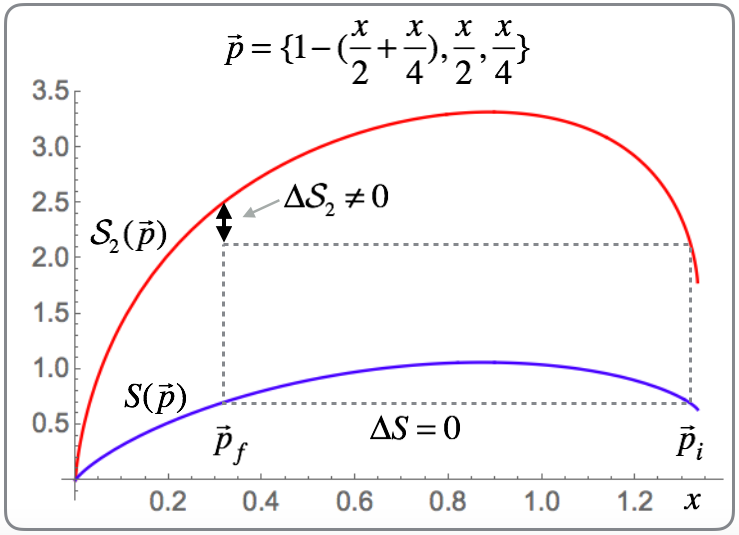
Figure 2: In systems with three or more levels it is possible to have very different distributions with the same Shannon entropy $S$. Thus, it is possible to have transformations for which the Shannon entropy does not change $S(\vec{p}_{f})-S(\vec{p}_{i})=0$, while other information measures such as $\mathcal{S}_{2}$ shown in the figure, do change $\mathcal{S}_{2}(\vec{p}_{f})-\mathcal{S}_{2}(\vec{p}_{i})\neq 0$.

V.3 Otto engine example: tighter than the second law

The last two examples have explicitly used the energy-information form the GCI. Next, we want to show that the GCI can also lead to strong results when using the periodic information-free form of the GCI (11).

It is not always sensible to compare the predictions of CI’s with different $\alpha$ since generally they contain information on different observables of the system. However, there are some interesting exceptions. One is the high temperature limit studied in Sec. III.1. Another exception occurs in two-level systems where all orders of heat are related to each other. Hence, any $\alpha$CI can be used to make a prediction on the standard $\mathcal{Q}_{1}$ heat.

From the $\alpha$ order heat definition (5) it follows that for isochore in a two-level system with energies $\{E_{1},E_{2}\}$:

$$\mathcal{Q}_{1}=\mathcal{Q}_{\alpha}\frac{E_{2}-E_{1}}{(E_{2}-F)^{\alpha}-(E_{1}-F)^{\alpha}}.$$ (40)

Using it the $\alpha$CI we get that

$$\mathcal{Q}_{1}\leq T^{\alpha}\Delta\mathcal{S}_{\alpha}\frac{E_{2}-E_{1}}{(E_{2}-F)^{\alpha}-(E_{1}-F)^{\alpha}}.$$ (41)

Now that for two-level system the GCI’s give predictions on the standard heat just like the regular second law we can compare them and see which one is tighter. As an example we consider the elementary heat machine shown in Fig. 3a. It is a four-stroke Otto machine with two levels as a working fluid. In the first stroke the system is cooled in an isochoric process (levels are fixed in time). In the second stroke work is invested. The third stroke is a hot isochore and the fourth is a work extraction stroke.

The efficiency of this machine is not difficult to calculate. However, our goal in this example is not to provide simpler methods for evaluating the efficiency, but to show to what extent thermodynamics puts a restriction on the efficiency of such an elementary device. The simplicity of the device shows that the impact of the GCI is not limited to complicated setups. Moreover in the low temperatures limit $T_{c}\ll E_{c,3}-E_{c,2},T_{h}\ll E_{h,3}-E_{h,2}$ any multi-level Otto machine (without level crossing in the adiabats) can be accurately modeled as a two-level Otto engine since the third level population is negligible.

Using (11) and (40) we get the efficiency bound

$$\eta\leq\eta_{\alpha CI}=1-\frac{T_{c}^{\alpha}}{T_{h}^{\alpha}}\frac{\frac{E_{c,2}-E_{c,1}}{(E_{c,2}-F_{c})^{\alpha}-(E_{c,1}-F_{c})^{\alpha}}}{\frac{E_{h,2}-E_{h,1}}{(E_{h,2}-F_{h})^{\alpha}-(E_{h,1}-F_{h})^{\alpha}}}$$ (42)

The parameters are $E_{c,2}-E_{c,1}=1$, $E_{h,2}-E_{h,1}=2$, $T_{c}=0.03$, $T_{h}=0.12$ and $F_{c(h)}=-T_{c(h)}\ln\sum\exp(-\beta_{c(h)}E_{j}^{c(h)})$ are the standard free energies. In Fig. 3b we see the actual efficiency (green line) of the engine, the Carnot bound $1-T_{c}/T_{h}$ from the standard second law (red line), and the GCI prediction for various $\alpha$ (blue curve). For $\alpha<1$ the $\alpha$CI prediction is significantly tighter compared to the standard Carnot bound. Since this machine is irreversible it is consistent to have a bound that is tighter than the Carnot efficiency.

When operating the same machine with colder temperatures $\{T_{c}^{\prime},T_{h}^{\prime}\}=\{T_{c},T_{h}\}/3$ the actual efficiency remains as it was before with $T_{c}$ and $T_{h}$ (Otto engine with uniform compression Uzdin and Kosloff (2014)). The Carnot bound $\eta_{Carnot}=1-T_{c}^{\prime}/T_{h}^{\prime}=1-T_{c}/T_{h}$ also remains the same. Yet, as shown by the dashed-magenta line in Fig. 3b, the $\alpha$CI efficiency bound converges to the actual efficiency for $\alpha\to 0$. It is both surprising and impressive that thermodynamic laws can predict the exact efficiency of an irreversible device. In appendix VII we show analytically that the $\alpha$CI (10) becomes tight in low temperatures

$$T_{c}^{\prime}\ll E_{c,2}-E_{c,1},T_{h}^{\prime}\ll E_{h,2}-E_{h,1}$$

and $\alpha\ll 1$ for Otto engines. This result is quite remarkable: we get a thermodynamic equality even though the machine is not in the reversible regime (where the crossover to the refrigerator takes place $T_{c}^{\prime}/T_{h}^{\prime}=\Delta E_{c}/\Delta E_{h}$ Uzdin and Kosloff (2014)) or in the linear response regime $T_{h}^{\prime}-T_{c}^{\prime}\ll T_{c}^{\prime}$.

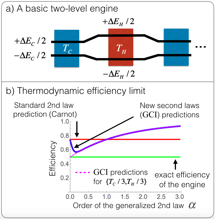
Figure 3: For a two-level four-stroke irreversible engine (a), the $\alpha<1$ order Clausius inequalities provides a tighter bound on the efficiency (blue curve in (b)), compared to the $\alpha=1$ standard Carnot efficiency bound (red line). The green line shows the exact efficiency of this engine. Remarkably, when both temperatures are decreased by the same factor (three in this example), the new $\alpha$CI bound (magenta) converges to the exact efficiency even though the machine is irreversible.

Next we wish to show how the $\alpha$CI can be used to study a new type of heat machine in which the standard second law does not provide any useful information.

V.4 Zero heat and half-zero heat machines

The flow of higher order heat in heat machines is a fascinating subject that goes beyond the scope of the present paper. However, to motivate this research direction, we describe a basic Otto “refrigerator” that reduces the energy variance of the cold bath without exchanging any (averaged) energy with it, i.e. $\mathcal{Q}_{1,c}=0$. We find that the performance of such machines is not limited by the standard $\alpha=1$ second law. In contrast, the $\alpha=2$ $\alpha$CI does put a concrete bound on the performance.

The machine we use is a four-stroke Otto machine (see Fig. 4a) that interacts with a cold bath in stroke I, and with a hot bath in stroke III. Some external work is applied to generate the adiabats in Stroke II and IV. The temperatures and the choice of energy levels needed to achieve $\mathcal{Q}_{1,c}=0$ are given in Appendix VIII.

The variance reduction in the cold bath is based on the fact that during the cold stroke $\mathcal{Q}_{2,c}>0$. Under the conditions in Appendix III, this implies that the bath experiences an energy variance reduction of $-\mathcal{Q}_{2,c}$. As pointed out earlier, in isochores with $\mathcal{Q}_{1}=0$, $\mathcal{Q}_{2}$ is equal to the change in energy variance.

While the energy flow (first order heat) to the cold bath is zero, the flow to the hot bath is not zero. From the standard $\alpha=1$ CI for periodic operation we get

$$-Q_{h}/T_{h}\geq 0,$$ (43)

which means that heat enters the hot bath as expected. Since the heat is zero for only one of the two baths, we call this device a “half-zero heat machine”. The energy that flows to the hot bath comes only from the work. This $\alpha=1$ result is plausible, but it provides no information on the changes in the cold bath, which concerns the main functionality of the device. On the other hand, the $\alpha=2$ CI (or other $\alpha$CI) for periodic operation yields

$$-\frac{\mathcal{Q}_{2,c}}{\mathcal{Q}_{2,h}}\leq\left(\frac{T_{c}}{T_{h}}\right)^{2},$$ (44)

in cases where $\mathcal{Q}_{2,h}\leq 0$. If $\mathcal{Q}_{2,h}$$>0$, the inequality sign has to be reversed. For the numerical values described in Appendix VIII, we get $-\mathcal{Q}_{2,c}/\mathcal{Q}_{2,h}\cong 0.234$, while the $\alpha=2$ CI sets a bound of $\left(\frac{T_{c}}{T_{h}}\right)^{2}=0.25$. By taking lower temperatures it is easy to approach the equality in (44), but then $\mathcal{Q}_{2,c}$ becomes very small. We conclude that the $\alpha=2$ GCI puts a realistic restriction on the performance of this machine. It determines what is the minimal amount of $\mathcal{Q}_{2}$ the hot bath must gain to remove $Q_{2,c}$ from the cold bath. This examples shows that there are cases where the GCI’s can provide information which is more important than that of the standard second law.

By using reversible state preparation protocol (LABEL:eq:_WR_berg), it is possible to construct a “full-zero heat machines” where both $\mathcal{Q}_{1,c}$ and $\mathcal{Q}_{1,h}$ are equal to zero (see Appendix VIII). In such machines (44) becomes an equality.

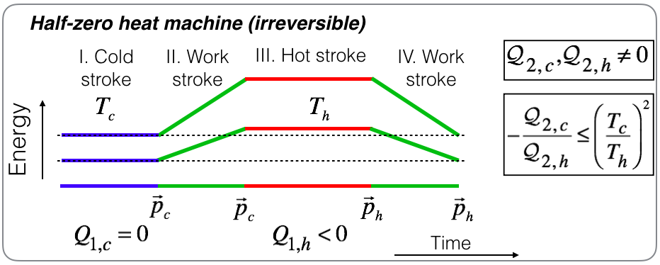
Figure 4: This “half zero” heat machine reduces the energy variance of the cold bath ($-\mathcal{Q}_{2,c}\leq 0$) without changing the average energy of the bath $\mathcal{Q}_{1,c}=0$. The standard Clausius inequality ($\alpha=1$) only predicts that the energy goes into the hot bath $\mathcal{Q}_{1,h}\leq 0$ but gives no information on the changes in the cold bath (which concerns the main functionality of the device). In contrast, the $\alpha=2$ GCI (10) predicts $-\mathcal{Q}_{2,c}/\mathcal{Q}_{2,h}\leq\left(T_{c}/T_{h}\right)^{2}$. In this example $-\mathcal{Q}_{2,c}/\mathcal{Q}_{2,h}\simeq 0.234$ while the GCI prediction is $\left(T_{c}/T_{h}\right)^{2}=0.25$.

The utility and practical value of such machines are outside the scope of the present paper. Here, the goal is only to show that with the $\alpha$CI, thermodynamics still imposes limitations on performance in such scenarios.

VI Concluding remarks

This paper presents generalized Clausius inequalities that establish new connections between information measures, energy moments, and the temperatures of the baths. As demonstrated, these laws lead to concrete new predictions in various physical setups. The energy-information structure of the GCI’s separates it from other extensions of the second law. In particular the GCI’s become equalities in reversible processes.

Since the GCI’s deal with non-extensive variables (higher moments of the energy) the information measures associated with these observables are not extensive as well. The scaling of the GCI with the system size in different setups is a fascinating topic that warrants further study. There are two possibilities: 1) All the GCI become trivial (predict $0\geq 0$) in the macroscopic limit. This would imply that the GCI’s are unique to the microscopic domain. 2) In the second scenario the GCI would provide information on tiny changes in macroscopic systems. Both alternatives will extend our understanding of thermodynamics and its scope.

The GCI’s have revealed some unexpected features both in hot temperatures, and in cold temperatures. The hot limit provided better information measures for estimation of standard heat. In cold temperatures we have seen that the GCI’s can predict the exact efficiency of an engine even though the engine is irreversible. These interesting GCI’s features should be further explored.

The regime of validity of the new laws can be smaller than that of the regular second law (which also has a regime of validity e.g. lack of initial system-bath correlation). It is a reasonable trade-off: the validity regime is potentially smaller but more information and more thermodynamic restrictions are available. In this work only part of the GCI validity regime has been mapped. The validity regime can be formulated in terms of “allowed operations”. We believe it is highly important to understand and map the full regime of validity. Based on numerical checks we conjecture that the regime of validity is significantly larger than the one we were able to deduce analytically at this point. Moreover, it is possible that some adaptations and refinements of the framework presented here will lead to a larger regime of validity.

Within this known regime of validity we provided explicit examples where the generalized Clausius inequality gives tighter and more useful constraints on the dynamics compared to the standard second law. A quantum extension was presented and used for providing a thermodynamic interpretation to various coherence measures. All the above-mentioned findings justify further work on this topic. The main goals are: 1) Finding additional predictions 2) Explore various limits (large $\alpha$, macroscopic limit, cold temperatures, etc.) 3) Extending the mapped regime of validity.

Moreover, it is interesting to extend the GCI formalism to other physical scenarios. For example, include chemical potentials in the GCI, and apply it to thermoelectric devices and molecular machines Kay and Leigh (2015). Another interesting option is to extend our findings to continuous distributions, and study dynamics of classical particles in a box (gas) from the point of view of the GCI’s. It is also interesting to study latent $\alpha$ heat in various phase transitions.

Appendix I - From Bregman divergences to generalized Clausius equalities

The Bregman divergence for a single-variable concave and differentiable function $\mathcal{S}(p)$ in the regime $p\in[0,1]$ is given by Bregman (1967)

$$D_{\mathcal{S}}^{B}(p,p_{ref}) =\mathcal{S}(p_{ref})-\mathcal{S}(p)+(p-p_{ref})(\partial_{p}\mathcal{S})|_{p=p_{ref}},$$ (45)

$$D_{\mathcal{S}}^{B}(p,p_{ref}) \geq 0,$$ (46)

where $p_{ref}$ is any point in $[0,1]$. The Bregman divergence, as shown in Fig. 5a, is the difference between a concave function and its linear extrapolation from point $p_{ref}$. Writing (45) again with $p\to p^{\prime}$ and subtracting (45) from it we get

$$\mathcal{S}(p^{\prime})-\mathcal{S}(p)-(p^{\prime}-p)\partial_{p}\mathcal{S}(p_{ref}) =D_{\mathcal{S}}^{B}(p,p_{ref})$$

$$-D_{\mathcal{S}}^{B}(p^{\prime},p_{ref}).$$ (47)

This equation also has a geometrical interpretation as shown in Fig. 5b. In particular, Fig 5b shows that when the final state is closer to the reference state from the same side, then the RHS of (47) is positive. To apply this for a probability distribution $\{p_{j}\}_{j=1}^{N}$ of $N$-level system we define

$$\mathcal{S}(\vec{p})=\sum_{j=1}^{N}\mathcal{S}(p_{j}),$$ (48)

and obtain a vector generalization of (47)

$$\mathcal{S}(\vec{p}\>^{\prime})-\mathcal{S}(\vec{p})-(\vec{p}\>^{\prime}-\vec{p})\cdot\nabla\mathcal{S}(\vec{p}_{ref}) =D_{\mathcal{S}}^{B}(\vec{p},\vec{p}_{ref})$$

$$-D_{\mathcal{S}}^{B}(\vec{p}\>^{\prime},\vec{p}_{ref}).$$ (49)

To apply this to thermodynamics we set $\vec{p}\>^{\prime}$ to be the final state of the system and $\vec{p}$ to be its initial state. The term $(\vec{p}\>^{\prime}-\vec{p})\cdot\nabla\mathcal{S}(\vec{p}_{ref})$ is a difference of two terms of the form $\sum p_{j}(\nabla\mathcal{S}(\vec{p}_{ref}))_{j}\triangleq\left\langle\nabla\mathcal{S}(\vec{p}_{ref})\right\rangle$ so $(\vec{p}\>^{\prime}-\vec{p})\cdot\nabla\mathcal{S}(\vec{p}_{ref})$ describes the change in the expectation value of the operator $\nabla\mathcal{S}(\vec{p}_{ref})$. Note that the operator does not depend on the initial and final distributions but only on the reference distribution $\vec{p}_{ref}$ that we will choose shortly. With this notations

$$\Delta\mathcal{S}-\Delta\left\langle\nabla\mathcal{S}(\vec{p}_{ref})\right\rangle=D_{\mathcal{S}}^{B}(\vec{p},\vec{p}_{ref})-D_{\mathcal{S}}^{B}(\vec{p}\>^{\prime},\vec{p}_{ref}).$$ (50)

This is still an identity that has nothing to do with thermodynamics. To get a Clausius-like inequality we want the RHS of (50) to be positive for thermodynamic process such as isochores, adiabats, and isotherms. As discussed in the main text, isochores can be used as a starting point. If the bath has a single fixed point so that the map it induces on the system $\vec{p}_{f}=M(\vec{p}_{i})$ satisfies $M(\vec{p}_{f.p.})=\vec{p}_{f.p.}$, we choose $\vec{p}_{ref}=\vec{p}_{f.p.}$. Since the goal of the bath is to bring the system closer to the fixed point, it is plausible that the RHS will be positive. However, although the bath may bring the state closer to the fixed point by some divergence measures, such as the relative entropy, it is not guaranteed that it will bring it closer when using the $D_{\mathcal{S}}^{B}$ as a proximity measure. Thus, one has to explore the regime of validity and check whether the given thermalization mechanism is “contractive under $D_{\mathcal{S}}^{B}$” (the RHS of (50) is positive). This is done in Sec. II.3.

For a single bath that is connected to all the levels of the system the fixed point is the thermal state so we set the reference state to be $p_{ref,j}=p_{\beta,j}=e^{-\beta(E_{j}-F)}$. For the choice $\partial_{p_{j}}\mathcal{S}(\vec{p})=(-\ln p_{j})^{\alpha}$ we get (7).

In addition, our formalism is also applicable to cases where different baths are connected to different parts of the system. These “parts”, that we call manifolds Uzdin et al. (2015), can either be in tensor product form when the system is composed of several particles, or in a direct sum form when different levels of the same particle are connected to baths with different temperatures. Such a scenario is common in microscopic heat machines (see Uzdin et al. (2015); Eitan Geva and Ronnie Kosloff (1994); Scovil and Schulz-DuBois (1959)).

The $k$ manifold of the system is associated with the part of the Hamiltonian $H_{k}=\sum_{j\in\{k\}}E_{j}\left|j\right\rangle\left\langle j\right|$ and it interacts with a bath of temperature $\beta_{k}$. The fixed point is $p_{ref,j}=p_{\vec{\beta},j}=e^{-\sum_{k}\beta_{k}(H_{k}-F_{k})}$ where $F_{k}$ are chosen so that each manifold has the correct total probability. If the manifolds share just one state then the fixed point is unique Uzdin et al. (2015). For the $\alpha$CI choice $\partial_{p}\mathcal{S}=(-\ln p)^{\alpha}$ we get

$$\Delta\mathcal{S}_{\alpha}-\sum_{k}\beta_{k}^{\alpha}\mathcal{Q}_{k,\alpha} = D_{\mathcal{S}}^{B}(\vec{p},\vec{p}_{\vec{\beta}})-D_{\mathcal{S}}^{B}(\vec{p}\>^{\prime},\vec{p}_{\vec{\beta}}),$$ (51)

$$\mathcal{Q}_{k,\alpha} = \Delta\left\langle(H-F_{k})^{\alpha}\right\rangle.$$ (52)

Equation (51) refers to isochores. For more general processes that include adiabats, isochores, and isotherms the derivation presented in the main text has to be repeated. In the regime of validity discussed in Sec. II.3, equation (51) yields

$$\Delta\mathcal{S}_{\alpha}-\sum_{k}\beta_{k}^{\alpha}\mathcal{Q}_{k,\alpha}\geq 0.$$ (53)

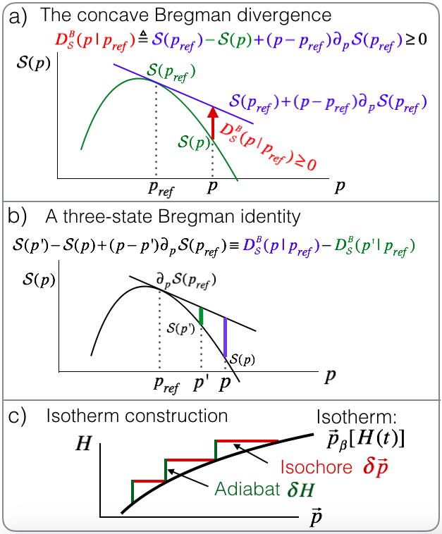
Figure 5: (a) The (concave) Bregman divergence has a simple geometric interpretation. It is the difference between the linear extrapolation of a concave function (blue) and the actual function (green). (b) A the three-state Bregman identity and its geometric interpretation. The right hand side determines the regime of validity of the generalized Clausius inequalities. Geometrically, it is the length of the blue line (initial divergence with respect to the reference) minus the length of the green line (final divergence with respect to the reference). If the final state is closer to the reference state (but does not overshoot to the other side) then the divergence difference is guaranteed to be positive as needed for the generalized Clausius inequalities. (c) By using concatenation of isochores and adiabats it is possible to construct various thermodynamic protocols that involve both heat and work such as isotherms. See text for the analysis.

Finally, we want to show how that the equality in the $\alpha$CI $\Delta\mathcal{S}_{\alpha}=\beta^{\alpha}\mathcal{Q}_{\alpha}$ is obtained for isotherms by using a concatenation of isochores and adiabats. This is an alternative derivation to (13). See Anders and Giovannetti (2013) for a similar analysis. Yet, here we carry out the calculation for the GCI and not only for the standard CI. Figure 5c shows a concatenation that approximates an isotherm $p_{\beta}[H(t)]$ (black curve). In the limit where the step size $\delta\vec{p}$ goes to zero the concatenation converges to the isotherm. We start at equilibrium and then perform a small change in the Hamiltonian $\delta H$ (green line). $\vec{p}$ remained fixed in this process so this is an adiabat (in particular, the entropy has not changed, and not heat was exchanged with the bath). So for the adiabat we get $\delta\mathcal{S}_{\alpha}=0,\delta\mathcal{Q}_{\alpha}=0$. Next we perform an isochore (red line) all the way to the ideal isotherm line. From (7) we get that for full thermalization ($\vec{p}_{f}=\vec{p}_{\beta}$) isochores

$$\delta\mathcal{S}_{\alpha}-\beta^{\alpha}\mathcal{Q}_{,\alpha}=D_{\mathcal{S}}^{B}(\vec{p}_{\beta}-\delta\vec{p},\vec{p}_{\beta})$$ (54)

By definition the term $\mathcal{Q}_{,\alpha}$ is linear in $\delta\vec{p}$. For the RHS we use a general property of the Bregman divergence $D_{\mathcal{S}}^{B}(\vec{p}-\delta\vec{p},\vec{p})=O(\delta\vec{p}^{2})$. This holds since $D_{\mathcal{S}}^{B}(\vec{p},\vec{p})=0$ and $D_{\mathcal{S}}^{B}(\vec{p}-\delta\vec{p},\vec{p})>0$ when $\delta\vec{p}\neq 0$. If there was a linear term, then by taking $\delta\vec{p}\to-\delta\vec{p}$ the divergence would have become negative when $\delta\vec{p}$ is very small. Figure 5a offers another way of understanding this property. The Bregman divergence is obtained from the function $\mathcal{S}$ by subtracting its linear extrapolator, and therefore it no longer has a linear term. Due this property we find that for the first stair in this staircase

$$\delta\mathcal{S}_{\alpha}^{(1)}=\beta^{\alpha}\delta\mathcal{Q}_{,\alpha}^{(1)}+O(\delta\vec{p}^{2}).$$ (55)

Repeating this for the $l$ stair and summing we find

$$\sum_{l}\delta\mathcal{S}_{\alpha}^{(l)}=\beta^{\alpha}\delta\mathcal{Q}_{,\alpha}^{(l)}+\sum_{l}O(\delta\vec{p}^{2}).$$ (56)

Since $\delta\mathcal{Q}_{,\alpha}^{(l)}=O(\delta\vec{p})$ then $\delta\mathcal{S}_{\alpha}^{(l)}$ must also be $O(\delta\vec{p})$ to balance the equation. The term $O(\delta\vec{p}^{2})$ becomes negligible in the limit $\delta\vec{p}\to 0$ and we get $\Delta\mathcal{S}_{\alpha}=\beta^{\alpha}\mathcal{Q}_{\alpha}$.

Appendix II - Reversible state preparation

In this appendix we derive (LABEL:eq:_WR_berg). Since we are interested now in reversible state preparation we can choose any reversible protocol that achieves the transformation $\{\vec{p}_{i},H_{i}\}\to\{\vec{p}_{f},H_{f}\}$.

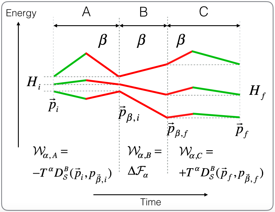
Figure 6: A three-stage reversible state-preparation protocol $\{\vec{p}_{i},H_{i}\}\to\{\vec{p}_{f},H_{f}\}$. Stage A changes the populations but the end point Hamiltonian is the same as the initial Hamiltonian. Stage B is an isotherm in which $H_{i}$ is changed to $H_{f}$. Finally, stage C changes the thermal state to the desired final state. This protocol is identical to state preparation with $\alpha=1$ but we monitor other quantities in the process ($\mathcal{W}_{\alpha}$ and $\mathcal{Q}_{\alpha}$). In this protocol the GCI’s become equalities and they give the exact amount of extracted $\mathcal{W}_{\alpha}$ and $\mathcal{Q}_{\alpha}$.

Figure 6 shows the protocol we chose for the derivation. Stage A implements the transformation $\{\vec{p}_{i},H_{i}\}\to\{\vec{p}_{\beta,i}=e^{-\beta(H_{i}-F_{i})},H_{i}\}$. Stage B is an isotherm $\{\vec{p}_{\beta,i},H_{i}\}\to\{\vec{p}_{\beta,f}=e^{-\beta(H_{f}-F_{f})},H_{f}\}$, and in stage C $\{\vec{p}_{\beta,f},H_{f}\}\to\{\vec{p}_{f},H_{f}\}$ is carried out. Starting with stage A we use (45) and (8) to write

$$T^{\alpha}\Delta\mathcal{S}_{\alpha,A}-\Delta\mathcal{H}_{\alpha,A} = T^{\alpha}D_{\mathcal{S}}^{B}(\vec{p}_{f},p_{\vec{\beta},f}).$$ (57)

Using $\mathcal{Q}_{\alpha,A}^{R}=T^{\alpha}\Delta\mathcal{S}_{\alpha,A}$ and the first law $\mathcal{Q}_{\alpha}^{R}-\Delta\mathcal{H}_{\alpha,A}=-\mathcal{W}_{\alpha,A}$, the reversible work extracted in the transformation $\{\vec{p}_{i},H_{i}\}\to\{\vec{p}_{\beta,i},H_{i}\}$ is

$$\mathcal{W}_{\alpha,A}=-T^{\alpha}D_{\mathcal{S}}^{B}(\vec{p}_{i},p_{\vec{\beta},i}).$$ (58)

Similarly, in stroke C (just the inverse of protocol used in A) the reversible work in $p_{\vec{\beta},f}$ to $\vec{p}_{f}$ is

$$\mathcal{W}_{\alpha,C}=+T^{\alpha}D_{\mathcal{S}}^{B}(\vec{p}_{f},p_{\vec{\beta},f}).$$ (59)

The last bit we need is the work in stage B. This is a pure isotherm so $\mathcal{Q}_{\alpha,B}=T^{\alpha}\Delta\mathcal{S}_{\alpha,B}$ and $\mathcal{W}_{\alpha,B}=[\mathcal{H}_{\alpha}(p_{\vec{\beta},f})-\mathcal{H}_{\alpha}(p_{\vec{\beta},i})]-T^{\alpha}[\mathcal{S}_{\alpha}(p_{\vec{\beta},f})-\mathcal{S}_{\alpha}(p_{\vec{\beta},f})]$. Therefore

$$\mathcal{W}_{\alpha,B} = \mathcal{F}_{\alpha}(\vec{p}_{\beta,f})-\mathcal{F}_{\alpha}(\vec{p}_{\beta,i})=\Delta\mathcal{F}_{\alpha},$$ (60)

$$\mathcal{F}_{\alpha} = \mathcal{H}_{\alpha}(\vec{p}_{\beta})-T^{\alpha}\mathcal{S}_{\alpha}(\vec{p}_{\beta}),$$ (61)

where $\mathcal{F}_{\alpha}$ is the equilibrium $\alpha$ free energy (no relation to the “$\alpha$ free energy” in thermodynamic resource theory). Adding the work contribution from all stages, we obtain that the total reversible work is given by (LABEL:eq:_WR_berg).

Appendix III - $\alpha$ order heat exchange with the bath

Our definition of heat and work can be considered as axioms. We define some observables of the system and put some thermodynamic constraints on how they can change in the spirit of the standard second law. Yet, in $\alpha=1$ thermodynamics the heat absorbed by the system is taken from the bath. To be more accurate, this is not always true since there might be some additional energy (work) needed to couple the system to the bath. In weak coupling this energy can be ignored but also in certain strong coupling cases Uzdin et al. (2016).

Nevertheless, regardless of where the energy goes, energy conservation implies that any energy change in the system is associated with an opposite change in the energy of the surroundings. Unfortunately, there is no general conservation law for $\mbox{$\mathcal{H}$}_{\alpha}$, so what can we learn on the change in the surroundings from the changes of $\mbox{$\mathcal{H}$}_{\alpha}$ in the system? We first focus on heat and in particular on isochores, and later discuss a specific yet important scenario of $\alpha$ work extraction.

VI.1 System-bath $\alpha$ heat flow

In our bath setup the bath consists of particles that can interact with the system and/or with each other (Fig. 7a). The Hamiltonian of the internal degrees of freedom of a particle $k$ in the bath is $H_{b,k}$. We make the following assumption

$$H_{b,k}=H_{s}+\sum_{m}e_{m}\left|m\right\rangle\left\langle m\right|.$$ (62)

That is, the bath particle has the same energy levels of the system plus (or minus) possibly additional levels $\left|m\right\rangle$ (see Fig. 7b). This is a reasonable assumption when the system resonantly interacts with the bath or when the bath particles and the system particle are of the same species. The setup studied here can describe various models. Several examples are shown in Fig. 7a: a collision bath model, a linear chain with nearest neighbor coupling, and all to all coupling geometry. For the interaction of the system with the bath particles, and of the bath particle between themselves, we assume a resonant “flip-flop” interaction term (Fig. 7b)

$$H_{int}=\sum_{j,k,l}c_{jk,l}\sigma_{j,l}^{-}\sigma_{k,l}^{+}+h.c.,$$ (63)

where $\sigma_{k,l}^{+}=\left|i+\omega_{l}\right\rangle\left\langle i\right|$ is the creation operator of energy gap $\omega_{l}$ in particle $k$, and $\sigma_{k,l}^{-}=(\sigma_{k,l}^{+})^{\dagger}$ is the corresponding annihilation operator. For simplicity, it is assumed that the gaps are non-degenerate so specifying $\omega_{l}$ specifies the state $\left|i\right\rangle$ as well. This two-particle interaction conserves the total bare energy $\left\langle H_{tot}\right\rangle=\left\langle H_{s}\right\rangle+\sum_{k}\left\langle H_{b,k}\right\rangle$, and it is very common in ion traps and in superconducting circuits (after making a justified rotating wave approximation). Furthermore, from $[H_{tot},H_{int}]=0$ that leads to energy conservation it also follows that $H_{tot}^{(\alpha)}$ is conserved where

$$\left\langle H_{tot}^{(\alpha)}\right\rangle\doteq\left\langle H_{s}^{\alpha}\right\rangle+\left\langle H_{b}^{(\alpha)}\right\rangle\doteq\left\langle H_{s}^{\alpha}\right\rangle+\sum_{k}\left\langle H_{b,k}^{\alpha}\right\rangle=\text{const}.$$ (64)

Note that $H_{b}^{(\alpha)}$ is equal to $H_{b}^{\alpha}\otimes I\otimes..+I\otimes H_{b}^{\alpha}\otimes..+..$ and not to $(H_{b}\otimes I\otimes..+I\otimes H_{b}\otimes..)^{\alpha}$. Interaction of the form (63) can only redistribute energy (or $\left\langle H^{(\alpha)}\right\rangle$) between system and bath. Hence, no extra work (or $W^{\alpha}$ work) is needed to couple the system and the bath.

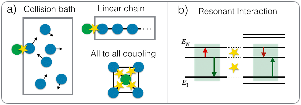
Figure 7: (a) Various system-bath configurations, and the interaction between elements (b). Each energy quanta taken from the bath particles is given to the system and vice versa. This type of interaction enables to easily relate changes in energy moments of the system, to changes in the bath.

When the bath and system particles are of the same species $F_{sys}=F_{bath}$ and it follows from (64) that $\Delta\left\langle\mathcal{H}_{b}^{(\alpha)}\right\rangle=-\Delta\left\langle\mathcal{H}_{sys}^{\alpha}\right\rangle$ or alternatively stated

$$\mathcal{Q}_{\alpha,b}=-\mathcal{Q}_{\alpha,sys}.$$ (65)

What happens $F_{s}\neq F_{bath}$? We go back to the motivation of defining of $\mathcal{H}_{sys}^{\alpha}$ as $(H-F)_{sys}^{\alpha}$. This followed from the Bregman divergence definition and from the fact that the Gibbs state is a fixed point of any thermalization map created by the bath. For the bath, these considerations are irrelevant. We can define $\mathcal{H}_{k}^{(\alpha)}$ of the k particle in the bath with any shift of interest. In particular, we can choose

$$\mathcal{H}_{b,k}^{\alpha}=(H_{b,k}-F_{sys})^{\alpha}.$$ (66)

With this choice we get $\Delta\left\langle\mathcal{H}_{b}^{(\alpha)}\right\rangle=-\Delta\left\langle\mathcal{H}_{sys}^{\alpha}\right\rangle$. For other observables such as $\left\langle e^{-(\tilde{\alpha}-1)\beta(H-F)}\right\rangle$ associated with the $\alpha$ impurity (see Sec. III) the relation is more straightforward. For any choice of $F_{b}$ we can use $\mathcal{Q}_{\tilde{\alpha}}=\left\langle e^{-(\tilde{\alpha}-1)\beta(H-F)}\right\rangle=e^{(\tilde{\alpha}-1)\beta F}\left\langle e^{-(\tilde{\alpha}-1)\beta H}\right\rangle$ and (64) and get

$$\mathcal{Q}_{\tilde{\alpha}}^{bath}=-e^{-(\tilde{\alpha}-1)\beta(F_{sys}-F_{b})}\mathcal{Q}_{\tilde{\alpha}}^{sys}.$$ (67)

The relation (67) holds for isochores. If the levels change in time a time integration over $\delta Q$ with $F_{sys}(t)$ has to be carried out.

In the bath models above the flip-flop interactions lead to multiple conservation laws. Consequently if some energy is exchanged with the bath and it is not in equilibrium anymore. Moreover, due to the conservation laws the bath will not equilibriate on its own once disconnected from the system. This is exactly the reason why it is important to keep track of higher order heat flow. They quantify the degradation of the bath. By assuming the bath is in a thermal state with unknown $\beta$ any knowledge of $\left\langle\mathcal{H}_{b}^{(\alpha)}\right\rangle$ can be used to get the correct $\beta$. However if the distribution is non thermal different $\alpha$ will produce different prediction for $\beta$. The $\beta$ mismatch is an indication for deviation of the bath from a thermal distribution.

VI.2 $\alpha$ Work

We now consider the case of applying a transient unitary on the system by driving it with $H_{s}(t)$. At the end of the pulse the Hamiltonian returns to its original value. In such scenarios the change in energy or in $\mathcal{H_{\alpha}}$ is only due to work ($\mathcal{W}_{\alpha}$). The problem is that in general it is not clear how a change of $\mathcal{W}_{\alpha}$ in the system is related to changes in the work repository. To simplify things we look at systems where specific two levels resonantly interact with a work repository. In the semi-classical limit the work repository is a harmonic oscillator in highly excited coherent state. This scenario is very useful in quantum heat machines Scovil and Schulz-DuBois (1959); Eitan Geva and Ronnie Kosloff (1994); Uzdin et al. (2015). The $\mathcal{W}_{\alpha}$ is

$$\mathcal{W}_{\alpha} =\sum_{j=\{k,l\}}(E_{j}-F)^{\alpha}dp_{j}$$

$$=[(E_{l}-F)^{\alpha}-(E_{k}-F)^{\alpha}]dp_{l}.$$ (68)

Since the regular work is $W=\mathcal{W}_{1}=(E_{l}-E_{k})dp_{l}$ we get a simple relation between work and $\alpha$ order work:

$$W=\frac{(E_{l}-E_{k})}{[(E_{l}-F)^{\alpha}-(E_{k}-F)^{\alpha}]}\mathcal{W}_{\alpha}.$$ (69)

In particular, in high temperature where $\left|F\right|\gg\left|E_{l}\right|,\left|E_{k}\right|$ we get: $W=\frac{(-F)^{1-\alpha}}{\alpha}\mathcal{W}_{\alpha}$. Surely, relation (69) does not provide a sufficient understanding of the operational effect of $\mathcal{W}_{\alpha}$ on the work repository, and further study on this topic is needed. Nevertheless, (69) is already sufficient to relate standard work to higher order heat flows $\mathcal{Q}_{\alpha}$ in certain classes of machines mentioned above.

Finally, we point out that there are thermodynamic scenarios like in absorption refrigerators where energy flows only in the form of heat, and there is no work at all.

Appendix IV - resource theory monotones

Like the generalized CI, thermodynamic resource theory (TRT) Goold et al. (2016); Horodecki and Oppenheim (2013); Brandão et al. (2015); Gour et al. (2015); Vinjanampathy and Anders (2016) also puts further restrictions on the interaction of a system with a thermal bath. Yet, as explained next, the similarities to the present framework seem to end there (note that the $\alpha$ index used in TRT has a completely different meaning). Both frameworks have their merits and deficiencies. In our view, both of them provide different tools for studying thermodynamic transformations at the microscopic scale.

Resource theory is the study of possible transformations from one state to the other, by using “free states” and possibly non-free states that are considered as a resource Goold et al. (2016); Vinjanampathy and Anders (2016); Gour et al. (2015). The free states in TRT are the thermal states. TRT is presently limited to scenarios with a single thermal bath (single temperature). In standard thermodynamics for a single bath, the CI can be replaced by the non-equilibrium free energy inequality

$$\Delta\tilde{F} \leq 0,$$ (70)

$$\tilde{F} = F+TD(p,p_{\beta}).$$ (71)

That is, $\tilde{F}$ is a monotone under certain thermodynamic transformations. Thermodynamic resource theory states that under “Thermal operations” Goold et al. (2016); Vinjanampathy and Anders (2016) the free energy is only one member of a whole monotone family Brandão et al. (2015):

$$\tilde{F}_{\breve{\alpha}} = F+TD_{\breve{\alpha}}(\vec{p},\vec{p}_{\beta}),$$ (72)

$$D_{\breve{\alpha}}(\vec{p},\vec{q}) = \frac{\text{sign}(\breve{\alpha})}{\breve{\alpha}-1}\ln\sum_{i}p_{j}^{\breve{\alpha}}q_{j}^{1-\breve{\alpha}}.$$ (73)

Where $\breve{\alpha}$ is a real number and $D_{\breve{\alpha}}(\vec{p},\vec{q})$ is the Rényi divergence (not to be confused with the Rényi entropy in (25), or with the Bregman divergence $D_{\bar{\alpha}}^{B}$ related to the Rényi entropy). If the initial state has coherences in the energy basis, then there are additional constraints Lostaglio et al. (2015a). What is remarkable about these thermodynamic monotones (72) is that they provide necessary and sufficient conditions for the existence of a thermal operation. That is, if all the monotones decrease in the transformation of two energy diagonal density matrices $\rho\to\sigma$, then a thermal operation that generates the transformation $\rho\to\sigma$ exists.

These thermodynamic monotones are sometimes referred to in the literature as “second laws”. The reasons that support this terminology are: 1) They have to decrease under thermal operation 2) The reduction of (72) to the standard (non-equilibrium) free energy (71) in the limit $\breve{\alpha}\to 1$. However, in our view the second law is more than a thermodynamic monotone. Consider the Clausius equality for isochores (7). The RHS is the monotone part of the equality, and it is positive in the regime of validity described in Sec. II.3. In traditional thermodynamics, it is the LHS that gives thermodynamics its strength. The LHS deals with thermodynamic quantities. In particular it has an energy-information structure.

In contrast, in TRT $\tilde{F}_{\breve{\alpha}}$ generally involves non-integer power of probabilities, and therefore cannot be directly related to observables. Presently, to the best of our knowledge, an operational thermodynamic meaning to $F_{\breve{\alpha}}$ for $\breve{\alpha}\neq 1$ (with the exclusion of $\tilde{F}_{\infty}$ and $\tilde{F}_{0}$ ) is still lacking (there is an informational state discrimination interpretation). In Funo and Ueda (2015) the $F_{\breve{\alpha}}$ are used to obtain an interesting $\breve{\alpha}$ independent result on the work fluctuation-dissipation trade-off with a single bath (“information engine” scenario - not a multiple bath heat engine scenario). See also Wilming and Gallego (2017); Woods et al. (2015) for different interesting directions of applying TRT.

More importantly, the TRT constraints (71) do not have an energy-information structure. The Rényi divergence $D_{\breve{\alpha}}(\vec{p},\vec{p}_{\beta})$ is a measure of distinguishability of a state $\vec{p}$ from the thermal state $\vec{p}_{\beta}$. However it is not a measure of the information content in the distribution $\vec{p}$. For example it is not even invariant to permutations in $\vec{p}$.

In summary, it seems that there is very little similarity between the GCI and TRT. Despite the differences, we hope that the TRT framework and the generalized CI framework can benefit from each other on the road to a deeper understanding of thermodynamics of small systems. As an example for exchange of ideas between the two formalisms, it is interesting to investigate the following question: we are given the transformation $\vec{p}\to\vec{q}$ and we find that $D_{\alpha}^{B}(\vec{p},\vec{p}_{\beta})\geq D_{\alpha}^{B}(\vec{q},\vec{p}_{\beta})$ for any $\alpha$, i.e. all the $\alpha$CI are satisfied. In analogy to thermal operation in TRT, does it imply that $\vec{p}\to\vec{q}$ can always be implemented with the allowed set of operations? The same question can be posed for other families of GCI’s such as the ones studied in Sec. III.

Appendix V - On the physicality of $\mathcal{S}_{\alpha}$

The goal of this section is not to enter the somewhat philosophical discussion on the physicality of information. It is clear that the Shannon entropy is a useful tool in stochastic thermodynamics, and in thermodynamics of small systems Seifert (2012). However, the Shannon entropy (or the von Neumann entropy) is not directly measurable. There is no Hermitian operator that corresponds to the entropy. In fact, the entropy is not even linear in the probabilities. This implies that in order to measure it, the probability distribution has to be measured via tomography.

Fortunately, in thermodynamics the standard CI provides a priceless connection between heat and entropy. For reversible, single-bath processes, the change in the entropy is given by $\Delta S_{sys}=Q/T$. Moreover, for irreversible isochores in the weak system bath coupling it holds that $\Delta S_{bath}=-Q/T_{bath}$ even when $\Delta S_{sys}\gg Q/T_{bath}$. In the $\alpha$CI the exact same thing holds. We can learn about the changes in $\Delta\mathcal{S}_{\alpha}$ from $\mathcal{Q}_{\alpha}/T^{\alpha}$. The reason why entropy is important is primarily because it can be related to heat, and secondly because we have some intuitive understanding of what are high and low entropy states. This however is true for any $\alpha$, not just $\alpha=1$. We conclude that in the context of the present paper $\mathcal{S}_{\alpha}$ is just as useful (or “physical”) as the regular Shannon entropy used in thermodynamics of small systems.

Appendix VI - An example of using coherence to extract higher order heat from a bath

We start this Appendix with a description of an irreversible protocol for extracting heat from a single bath using coherence erasure (the protocol in Kammerlander and Anders (2016) is reversible).

In step A of the protocol a pulse (unitary operation) is applied to bring the system into a passive state (no coherence and no population inversion in the energy basis). The new probabilities in the energy basis are $p_{i}^{\prime}$. In step B we change the energy level $E_{i}$ without interacting with the bath to $E_{i}=-T\log p_{i}$. In step C a full isochoric thermalization take place so the density matrix is equal to $\rho_{\Lambda}$ . Finally, in step D the bath is disconnected and the levels are adiabatically restored to their original value $E_{i}$.

In this protocol $\mathcal{Q}_{\alpha}<T^{\alpha}D_{\alpha}^{B}(\rho,\rho_{\Lambda})$. Since the thermal interaction in this protocol protocol is an isochore, it is easy to relate it to changes in the bath moments (see Appendix III). As a concrete example we consider a qutrit system that is initially in a state

$$\rho_{s,0}=\left(\begin{array}[]{ccc}\nicefrac{{1}}{{6}}&\nicefrac{{1}}{{400}}&0\\ \nicefrac{{1}}{{400}}&\nicefrac{{1}}{{3}}&\nicefrac{{1}}{{20}}\\ 0&\nicefrac{{1}}{{20}}&\nicefrac{{1}}{{2}}\end{array}\right).$$

The reason for choosing small coherence values is that we want start close to thermal equilibrium in order to show that the higher order bound (36) can produce a reasonably tight bound. The diagonals correspond to thermal distribution with temperature of 1 and a Hamiltonian $H=diagonal[\{\ln 3,\ln\tfrac{3}{2},0\}]$. Since the populations are already in thermal form (Gibbs state) the irreversible protocol described above, has only two stages: a unitary rotation pulse (stage A), and an isochore (stage C).

For stage A we apply an interaction Hamiltonian (in the interaction picture)

$$H_{int}=\left(\begin{array}[]{ccc}0&+i&0\\ -i&0&-i\\ 0&+i&0\end{array}\right),$$

and find that at some point in time ($t_{f}\simeq 0.204$), $\left\langle H\right\rangle_{t_{f}}=\left\langle H\right\rangle_{t_{0}}$. At time $t_{f}$ we start stage C (an isochore). As a result, there is no heat exchange with the bath. Since the $\mathcal{Q}_{1}=0$, $\mathcal{Q}_{2}$ expresses the change in energy variance. In this example $\mathcal{Q}_{2}\geq 0$ which implies, under the condition in Appendix III, that the energy variance of the particles in the bath is decreasing.

The bound (36) on the change in variance yields a value that is 1.92 times large than the actual change in the energy variance.

Appendix VII - The low temperature limit

The goal of this appendix is to explain and show analytically why the GCI prediction for cold temperature and $\alpha\to 0$, converges to the exact efficiency of the Otto machine (Sec. V.3 and dashed curve in Fig. 3b). For hot isochore of the Otto machine the GCI reads:

$$\Delta\mathcal{S}_{\alpha}^{h}-\beta_{h}^{\alpha}\mathcal{Q}_{\alpha}^{h} \geq 0$$ (74)

Let us write the initial state as

$$\vec{p}_{c}=\vec{p}_{h}-d\vec{p}$$

In full thermalization isochores, there are different scenarios in which $d\vec{p}$ can be small. For example, close to the crossover to refrigerator $T_{c}/T_{h}=\Delta E^{c}/\Delta E^{h}$ where the machine becomes reversible, $d\vec{p}$ is very small (at the crossover the Otto machine satisfies $d\vec{p}=0$ and it produces zero work per cycle, e.g. see Uzdin and Kosloff (2014)). Another scenario takes place when $T_{c}\ll\Delta E^{c},T_{h}\ll\Delta E^{h}$. Most of the population is in the ground state and $\vec{p}_{c}$ and $\vec{p}_{h}$ differ by a very small number $\exp(-\beta_{c}\Delta E^{c})-\exp(-\beta_{h}\Delta E^{h})$. However, $T_{c}$ and $T_{h}$ are very different from each other (not linear response) and very different from the refrigerator crossover point $T_{c}/T_{h}\neq\Delta E^{c}/\Delta E^{h}$. Since the Carnot bound also converge to the actual efficiency near the refrigerator crossover (first scenario), we are interested here only in the second scenario where both temperatures are low but still very different from each other or from the refrigerator crossover ratio. Expanding both terms in (74) in powers of $\alpha$ and $d\vec{p}$ yields

$$\Delta\mathcal{S}_{\alpha}^{h} =\alpha\sum_{j}dp_{j}\ln[-\ln[p_{h,j}]]+O(dp_{j}^{2},\alpha^{2}),$$ (75)

$$\beta_{h}^{\alpha}\mathcal{Q}_{\alpha}^{h} =\alpha\sum_{j}dp_{j}\ln[-\ln[p_{h,j}]]+O(dp_{j}^{2},\alpha^{2}).$$ (76)

The higher order terms $O(dp_{j}^{2},\alpha^{2})$ in (75) and (76) differ from each other. From (75) and (76) we conclude that when both $dp_{j}$ and $\alpha$ are small, the two terms in (74) cancel each other in the lowest order of $\alpha$ and $d\vec{p}$. Thus, the $\alpha$CI holds as an equality in the limit $d\vec{p}\ll 1,\alpha\ll 1$. This explains why the $\alpha$CI prediction (dashed-blue line in Fig. 3) converges to the actual efficiency although irreversible processes (isochores) are involved. We point out that on top of low temperatures $\alpha\ll 1$ is also required for (74) to become equality. For large $\alpha$ the $O(\alpha^{2})$ terms become important and the $\alpha$CI is no longer tight.

Appendix VIII - choice of parameters for a half-zero heat machine

In this appendix we describe how to choose the energy levels of the machine in Fig. 4 in order to achieve $\mathcal{Q}_{1,c}=0$. The cold levels can be chosen freely and we set them to be $E_{c}=\{0,1,2\}$. For simplicity, it is assumed that the baths are connected for a period which exceeds several thermalization times. Hence, at the end of stroke I the populations are $p_{c,j}=e^{-\beta_{c}(E_{c,j}-F_{c})}$. The cold and hot bath temperatures are $\{T_{c},T_{h}\}=\{0.5,1\}$. To determine the hot levels, we first choose what is the distribution $\vec{p}_{h}$ we want the hot bath to generate. To achieve $\mathcal{Q}_{1,c}=(\vec{p}_{h}-\vec{p}_{c})\cdot\vec{E}_{c}=0$ we set $\vec{p}_{h}=\vec{p}_{c}+\{-1,2,-1\}\delta p$ where $\delta p$ is taken to be $\delta p=p_{c}(3)/20$. Consequently, the hot energy levels are $\vec{\mathcal{E}}{}_{h}=\vec{E}_{h}-F_{h}=-T_{h}\ln\vec{p}_{h}$. Choosing one of the levels will fix $F_{h}$ and the values of all the hot levels. By setting $E_{h,1}=0$ we get $E_{h}\simeq\{0,1.986,4.05\}.$ Nevertheless, for calculating heat (of any order) only $\vec{\mathcal{E}}{}_{h}$ is needed.

To obtain a full zero machine with $Q_{c}=Q_{h}=0$ we choose two states $\vec{p}_{A,}\vec{p}_{B}$ that have the same Shannon entropy (at least three levels are needed. See Fig. 2 for an example). A reversible state preparation is used to prepare $\vec{p}_{B}$ from $\vec{p}_{A}$ using a bath in temperature $T_{c}$, and another reversible state preparation is used to create $\vec{p}_{A}$ from $\vec{p}_{B}$ using a bath in temperature $T_{h}$.

References

- Alicki (1979) R. Alicki, J. Phys A: Math.Gen. 12, L103 (1979).
- Sagawa (2012) T. Sagawa, Lectures on Quantum Computing, Thermodynamics and Statistical Physics 8, 127 (2012).
- Peres (2006) A. Peres, Quantum theory: concepts and methods, Vol. 57 (Springer Science & Business Media, 2006).
- Esposito and Van den Broeck (2011) M. Esposito and C. Van den Broeck, EPL (Europhysics Letters) 95, 40004 (2011).
- Uzdin et al. (2015) R. Uzdin, A. Levy, and R. Kosloff, Phys. Rev. X 5, 031044 (2015).
- Gelbwaser-Klimovsky and Kurizki (2014) D. Gelbwaser-Klimovsky and G. Kurizki, Physical Review E 90, 022102 (2014).
- Mitchison et al. (2015) M. T. Mitchison, M. P. Woods, J. Prior, and M. Huber, New Journal of Physics 17, 115013 (2015).
- Andrieux and Gaspard (2008) D. Andrieux and P. Gaspard, Proceedings of the National Academy of Sciences 105, 9516 (2008).
- Jarzynski (2008) C. Jarzynski, Proceedings of the National Academy of Sciences 105, 9451 (2008).
- Seifert (2012) U. Seifert, Reports on Progress in Physics 75, 126001 (2012).
- Harris and Schütz (2007) R. Harris and G. Schütz, Journal of Statistical Mechanics: Theory and Experiment 2007, P07020 (2007).
- Jarzynski (2011) C. Jarzynski, Annu. Rev. Condens. Matter Phys. 2, 329 (2011).
- Roßnagel et al. (2016) J. Roßnagel, S. T. Dawkins, K. N. Tolazzi, O. Abah, E. Lutz, F. Schmidt-Kaler, and K. Singer, Science 352, 325 (2016).
- Maslennikov et al. (2017) G. Maslennikov, S. Ding, R. Hablutzel, J. Gan, A. Roulet, S. Nimmrichter, J. Dai, V. Scarani, and D. Matsukevich, arXiv preprint arXiv:1702.08672 (2017).
- Niskanen et al. (2007) A. Niskanen, Y. Nakamura, and J. Pekola, Physical Review B 76, 174523 (2007).
- Campisi et al. (2015) M. Campisi, J. Pekola, and R. Fazio, New Journal of Physics 17, 035012 (2015).
- Gelbwaser-Klimovsky and Kurizki (2015) D. Gelbwaser-Klimovsky and G. Kurizki, Scientific reports 5 (2015).
- Zhang et al. (2014) K. Zhang, F. Bariani, and P. Meystre, Physical review letters 112, 150602 (2014).
- Mitchison et al. (2016) M. T. Mitchison, M. Huber, J. Prior, M. P. Woods, and M. B. Plenio, Quantum Science and Technology 1, 015001 (2016).
- Jarzynski (1999) C. Jarzynski, Journal of Statistical Physics 96, 415 (1999).
- Quan and Dong (2008) H. Quan and H. Dong, arXiv preprint arXiv:0812.4955 (2008).
- Campisi (2014) M. Campisi, J. Phys A: Math.theor. 47, 245001 (2014).
- Goold et al. (2016) J. Goold, M. Huber, A. Riera, L. del Rio, and P. Skrzypczyk, Journal of Physics A: Mathematical and Theoretical 49, 143001 (2016).
- Horodecki and Oppenheim (2013) M. Horodecki and J. Oppenheim, Nature communications 4, 2059 (2013).
- Gour et al. (2015) G. Gour, M. P. Müller, V. Narasimhachar, R. W. Spekkens, and N. Y. Halpern, Physics Reports 583, 1 (2015).
- Lostaglio et al. (2015a) M. Lostaglio, D. Jennings, and T. Rudolph, Nature communications 6, 6383 (2015a).
- Lostaglio et al. (2015b) M. Lostaglio, M. P. Müller, and M. Pastena, Phys. Rev. Lett. 115, 150402 (2015b).
- Deffner and Lutz (2010) S. Deffner and E. Lutz, Physical review letters 105, 170402 (2010).
- Anders and Giovannetti (2013) J. Anders and V. Giovannetti, New Journal of Physics 15, 033022 (2013).
- Bregman (1967) L. M. Bregman, USSR computational mathematics and mathematical physics 7, 200 (1967).
- Still et al. (2012) S. Still, D. A. Sivak, A. J. Bell, and G. E. Crooks, Physical review letters 109, 120604 (2012).
- Reeb and Wolf (2014) D. Reeb and M. M. Wolf, New Journal of Physics 16, 103011 (2014).
- Note (1) Follow immediately from the convexity of and the fact that a linear term does not affect concavity.
- Spohn (1978) H. Spohn, Journal of Mathematical Physics 19, 1227 (1978).
- H.-P. Breuer and F. Petruccione (2002) H.-P. Breuer and F. Petruccione, Open quantum systems (Oxford university press, 2002).
- A. E. Allahverdyan, R. Balian, and Th. M. Nieuwenhuizen (2004) A. E. Allahverdyan, R. Balian, and Th. M. Nieuwenhuizen, Euro. Phys. Lett. 67, 565 (2004).
- Havrda and Charvát (1967) J. Havrda and F. Charvát, Kybernetika 3, 30 (1967).
- Vajda (1968) I. Vajda, Kybernetika 4, 105 (1968).
- Daróczy (1970) Z. Daróczy, Information and control 16, 36 (1970).
- Tsallis (1988) C. Tsallis, Journal of statistical physics 52, 479 (1988).
- Abe and Okamoto (2001) S. Abe and Y. Okamoto, Nonextensive statistical mechanics and its applications, Vol. 560 (Springer Science & Business Media, 2001).
- Note (2) Purity is defined and we call one minus the purity the “impurity” of . The impurity is best known as Tsallis entropy. However, the physical context of Tsallis entropy is associated with non thermal Tsallis distribution. Since our reservoirs are always thermal we use a different name to prevent possible confusion.
- Nock et al. (2013) R. Nock, B. Magdalou, E. Briys, and F. Nielsen, in Matrix Information Geometry (Springer, 2013) pp. 373–402.
- Molnár et al. (2016) L. Molnár, J. Pitrik, and D. Virosztek, Linear Algebra and its Applications 495, 174 (2016).
- Note (3) We use the Bregman divergence only for density matrices. Hence, conjugation and transposition are not needed.
- Baumgratz et al. (2014) T. Baumgratz, M. Cramer, and M. Plenio, Physical review letters 113, 140401 (2014).
- Kammerlander and Anders (2016) P. Kammerlander and J. Anders, Scientific Reports 6, 22174 (2016).
- Uzdin and Kosloff (2014) R. Uzdin and R. Kosloff, New Journal of Physics 16, 095003 (2014).
- Kay and Leigh (2015) E. R. Kay and D. A. Leigh, Angewandte Chemie International Edition 54, 10080 (2015).
- Eitan Geva and Ronnie Kosloff (1994) Eitan Geva and Ronnie Kosloff, Phys. Rev. E 49, 3903 (1994).
- Scovil and Schulz-DuBois (1959) H. E. D. Scovil and E. O. Schulz-DuBois, Phys. Rev. Lett. 2, 262 (1959).
- Uzdin et al. (2016) R. Uzdin, A. Levy, and R. Kosloff, Entropy 18, 124 (2016).
- Brandão et al. (2015) F. Brandão, M. Horodecki, N. Ng, J. Oppenheim, and S. Wehner, Proceedings of the National Academy of Sciences 112, 3275 (2015).
- Vinjanampathy and Anders (2016) S. Vinjanampathy and J. Anders, Contemporary Physics 57, 545 (2016).
- Funo and Ueda (2015) K. Funo and M. Ueda, Physical review letters 115, 260601 (2015).
- Wilming and Gallego (2017) H. Wilming and R. Gallego, arXiv preprint arXiv:1701.07478 (2017).
- Woods et al. (2015) M. P. Woods, N. Ng, and S. Wehner, arXiv preprint arXiv:1506.02322 (2015).