The discovery of a planetary candidate around the evolved low-mass Kepler giant star HD 175370

Abstract

We report on the discovery of a planetary companion candidate with a minimum mass $M\,\sin i=4.6\pm 1.0\,M_{\rm{Jupiter}}$ orbiting the K2 III giant star HD 175370 (KIC 007940959). This star was a target in our program to search for planets around a sample of 95 giant stars observed with Kepler. This detection was made possible using precise stellar radial velocity measurements of HD 175370 taken over five years and four months using the coudé echelle spectrograph of the 2-m Alfred Jensch Telescope and the fibre-fed echelle spectrograph HERMES of the 1.2-m Mercator Telescope. Our radial velocity measurements reveal a periodic ($349.5\pm 4.5$ days) variation with a semi-amplitude $K=133\pm 25\,\rm{m\,s^{-1}}$, superimposed on a long-term trend. A low-mass stellar companion with an orbital period of $\sim 88$ years in a highly eccentric orbit and a planet in a Keplerian orbit with an eccentricity $e=0.22$ are the most plausible explanation of the radial velocity variations. However, we cannot exclude the existence of stellar envelope pulsations as a cause for the low-amplitude radial velocity variations and only future continued monitoring of this system may answer this uncertainty. From Kepler photometry we find that HD 175370 is most likely a low-mass red-giant branch or asymptotic-giant branch star.

1 Introduction

Planets around K-giant stars may provide us with clues on the dependence of planet formation on stellar mass. The progenitors of K-giant stars are often intermediate-mass main-sequence A-F stars. While on the main sequence these stars are not amenable to precise radial velocity (RV) measurements. There is a paucity of stellar lines due to high effective temperatures and these are often broadened by rapid rotation. Therefore one cannot easily achieve the RV precision needed for the detection of planetary companions. On the other hand, when these stars evolve to giant stars they are cooler and have slower rotation rates and a RV accuracy of a few$\,\,\rm{m\,s^{-1}}$ can readily be achieved. The giant stars thus serve as proxies for planet searches around intermediate-mass (1.2–2 $M_{\odot}$) early-type main-sequence stars.

Since the discovery of the first exoplanet around K-giant stars (Hatzes & Cochran, 1993; Frink et al., 2002), over 90 exoplanets (3 per cent of the total in September 2016) have been discovered orbiting giant stars. These planet-hosting giant stars are on average more massive than planet-hosting main-sequence stars. Johnson et al. (2010) showed, based on an empirical correlation, that the frequency of giant planets increases with stellar mass to about 14 per cent for A-type stars. This is consistent with theoretical predictions of Kennedy & Kenyon (2008), who concluded that the probability that a given star has at least one gas giant increases linearly with stellar mass from 0.4 to 3 $M_{\odot}$. Statistical analysis of microlensing and transiting data reveals that cool Neptunes and super-Earths are even more common than Jupiter-mass planets (Cassan et al., 2012; Howard et al., 2012).

Unlike for a main-sequence star where there is more or less a direct mapping between effective temperature and stellar mass, it is more problematic to determine the stellar mass of a giant star. The evolutionary tracks for stars covering a wide range of masses all converge to the similar region of the H-R diagram. One way to obtain the stellar mass is to rely on evolutionary tracks. However, they are not only model dependent, but they require accurate stellar parameters such as the effective temperature and heavy element abundance. Lloyd (2011) argued that the masses of giant stars in Doppler surveys were only in the range 1.0 – 1.2 $M_{\odot}$ and thus were not intermediate-mass stars. Clearly, we cannot disentangle the effect of stellar mass on the observed planet properties if we cannot get a reliable measurement of the stellar mass.

The stellar mass can be derived from solar-like oscillations. The first firm discovery of solar-like oscillations in a giant star was made using RVs by Frandsen et al. (2002). However, it was only recently that solar-like oscillations were unambiguously found in late-type giant stars, owing to space-based photometric observations by the CoRoT (De Ridder et al., 2009) and the Kepler (Gilliland et al., 2010) missions. Solar-like p-mode oscillations of the same degree are equally spaced in frequency and the spacing is related to the square root of the mean stellar density ($\propto$$(M/R^{3})^{1/2}$), whereas the frequency of maximum oscillation power is $\propto$ $M/(R^{2}\sqrt{T_{\rm{eff}}})$ (Kjeldsen & Bedding, 1995). From these empirical relations we can calculate both the stellar mass and radius in a more or less model independent way.

The Kepler Space Mission has been monitoring a sample of over 13,000 red-giant stars which can be used for asteroseismic studies. All stars show stellar oscillations that have been analysed to determine their fundamental stellar parameters (Huber et al., 2010; Stello et al., 2013) and internal stellar structure (Bedding et al., 2011). Furthermore, an estimate of the stellar age can be obtained using stellar models (Lebreton & Goupil, 2014).

Giant stars observed with Kepler represent a unique sample for planet searches as a planetary detection would mean that we can determine reliable stellar properties via asteroseismic analysis, characteristics not well known for many other planet-hosting giant stars. For this reason, we started a planet-search program among Kepler asteroseismic-giant stars in 2010. We have distributed our targets over four different telescopes in order to maximize the detection and to minimize the impact of telescope resources at a single site. These telescopes include the 2-m telescope at Thüringer Landessternwarte Tautenburg (TLS), Germany (29 stars, since 2010), the 1.2-m Mercator telescope, La Palma, Spain (38 stars, since 2011), the 2.5-m Nordic Optical Telescope, La Palma, Spain (12 stars, since 2012) and the 2.7-m telescope at McDonald Observatory, Texas, US (33 stars, since 2012). In total our sample contains 95 giant stars, a statistically significant number given an expected detection rate of $\sim$15 per cent. We observe some targets in common at different sites, in order to check our measurements independently.

Until now, three Kepler giant stars are known to harbor planets discovered by detecting transits in the Kepler light curves. Huber et al. (2013) found two planets in the Kepler-56 system, while Lillo-Box et al. (2014) confirmed the hot-Jupiter Kepler-91 b. Ciceri et al. (2015), Ortiz et al. (2015) and Quinn et al. (2015) discovered the warm Jupiter Kepler-432 b. An additional planetary candidate has also been reported to Kepler-432 (Quinn et al., 2015) and Kepler-56 (Otor et al., 2016) found via a long-term RV monitoring. Here, we report on the discovery of a giant planetary candidate orbiting the K-giant star HD 175370 (KIC 007940959) in the Kepler field found via the RV method.

2 Observations and data analysis

We have observed HD 175370 since March 2010 using the coudé echelle spectrograph at the 2-m Alfred Jensch Telescope of the TLS, Germany. We obtained 28 spectra with a S/N of $\sim$ 100 per pixel in the extracted spectrum. Since May 2011 we have monitored this star using the fibre-fed High Efficiency and Resolution Mercator Echelle Spectrograph (HERMES) at the 1.2-m Mercator Telescope on La Palma, Canary Islands, Spain. We obtained 23 spectra with a S/N of $\sim$ 85 per pixel in the extracted spectrum. The RV measurements from both sites are listed in Table 1.

Table 1: RV and bisector velocity span (BVS) measurements of HD 175370 (see section 5.2 for more details). The RVs were corrected for the barycenter motion. The RV uncertainty shown here is an instrumental error.

BJD	RV	$\sigma_{\rm{RV}}$	BVS	$\sigma_{\rm{BVS}}$
(d)	($\rm{m\,s^{-1}}$)	($\rm{m\,s^{-1}}$)	($\rm{m\,s^{-1}}$)	($\rm{m\,s^{-1}}$)
TLS RVs
2455278.532376	-605.8	35.2
2455278.602766	-542.6	8.3
2455353.365205	-471.7	8.6
2455451.296195	-328.7	8.0
2455483.272526	-346.7	8.7
2455488.271606	-353.9	7.6
2455494.400977	-365.2	6.8
2455666.577048	-353.7	8.7
2455670.502131	-344.5	8.6
2455677.567170	-325.1	10.1
2455761.388294	-158.0	8.5
2455849.373157	-219.0	7.9
2456046.423323	-54.4	14.0
2456051.588440	-9.1	11.1
2456057.491668	-4.4	11.3
2456090.435786	70.9	9.3
2456096.490665	95.0	8.0
2456101.446685	139.5	10.0
2456167.316765	8.5	10.0
2456169.423236	47.4	7.8
2456229.271206	-163.6	11.5
2456253.219143	-169.0	8.2
2456407.417441	202.3	10.2
2456412.527780	202.1	7.9
2456458.380429	217.1	8.3
2456461.561057	256.1	7.7
2456496.364666	309.4	9.1
2456549.517513	187.0	7.2
HERMES RVs
2455685.659388	-13286	5	86	7
2455770.401373	-13218	6	111	6
2455790.522891	-13185	6	103	8
2456039.673779	-13100	5	80	8
2456125.521027	-12964	6	105	8
2456160.424115	-13010	6	109	7
2456397.618813	-12816	7	124	7
2456457.504014	-12685	6	112	7
2456555.460851	-12765	9	105	7
2456564.427449	-12758	11	132	6
2456565.448662	-12786	8	67	5
2456598.291663	-12929	10	139	7
2456604.286132	-12882	8	106	9
2456607.290885	-12966	10	194	9
2456754.705837	-12684	7	82	7
2456804.590638	-12657	10	184	6
2456846.419078	-12705	7	97	7
2456884.486310	-12584	10	67	6
2457212.518734	-12497	12	233	7
2457214.736763	-12532	9	88	11
2457219.738180	-12534	7	119	10
2457220.734581	-12513	9	149	9
2457222.643519	-12487	8	153	8

The coudé echelle spectrograph at TLS provides a wavelength range of 4670 – 7400 Å and a spectral resolution of 67,000. We have reduced the data using standard IRAF procedures (bias subtraction, flat-field correction, extraction of individual echelle orders, wavelength calibration, subtraction of scattered light, cosmic rays removal and spectrum normalization). The wavelength reference for the RV measurements was provided by an iodine absorption cell placed in the optical path just before the slit of the spectrograph. The calculation of the RVs largely followed the method outlined in Valenti, Butler & Marcy (1995), Butler et al. (1996) and Endl, Kürster & Els (2000), and takes into account changes in the instrumental profile. We note that the measured RVs are relative to a stellar template which is an iodine-free spectrum (see Table 1) and are not absolute values.

For the HERMES spectrograph, we used a simultaneous ThArNe wavelength reference mode and low-resolution fibre (LRF) in order to achieve as accurate RV measurements as possible. The LRF mode has a spectral resolution of 62,000 and HERMES has a wavelength range of 3770 – 9000 Å. More details about the HERMES spectrograph can be found in Raskin et al. (2011). We have used a dedicated automated data reduction pipeline and RV toolkit (HermesDRS) to reduce the data and calculate absolute RVs (see Table 1). The spectral mask of Arcturus on the velocity scale of the IAU RV standards was used for the cross-correlation.

The two data sets (relative TLS and absolute HERMES RVs) were combined adjusting their zero points during the orbital fitting procedure as described in section 4.

3 Properties of the star HD 175370

HD 175370 (KIC 007940959) has a visual magnitude of $m_{V}=7.19$ mag (Høg et al., 2000). The parallax was determined by van Leeuwen (2007) from Hipparcos data as $3.68\pm 0.45$ mas which implies an absolute magnitude $M_{V}=0.02\pm 0.27$ mag. Table 2 lists the stellar parameters of HD 175370 known from literature together with those determined in this work.

Table 2: Stellar parameters of HD 175370. The top part of the table lists parameters that are derived using spectral analysis or calculated in this paper, unless stated otherwise. The central part of the table shows resulting parameters from asteroseismic analysis. The bottom part of the table lists derived parameters using GBM modelling as described in section 3.2. We show parameters for the red-giant branch (RGB), red clump (RC) and asymptotic-giant branch (AGB) star. The probability for each evolutionary phase gives the total integrated likelihood of the distributions.

Parameter	Value			Unit
$m_{V}^{a}$	$7.19\pm 0.01$			mag
$B-V^{a}$	$1.27\pm 0.02$			mag
Parallaxb	$3.68\pm 0.45$			mas
$M_{V}$	$0.02\pm 0.27$			mag
Distance	$272\pm 33$			pc
Spectral type	K2 III
$T_{\rm{eff}}$	$4301\pm 43$			K
$[\rm{Fe/H}]$	$-0.52\pm 0.07$			dex
$v_{\rm{turb}}$	$1.63\pm 0.13$			$\rm{km\,s^{-1}}$
$v\,\sin i$	$6.11\pm 0.50$			$\rm{km\,s^{-1}}$
$\log g$	$1.70\pm 0.15$			dex
$\Delta\nu$	$6.7\pm 0.2$			$\mu$Hz
$\nu_{\rm max}$	$1.17\pm 0.03$			$\mu$Hz
	RGB star	RC star	AGB star
$\log g$	$1.70\pm 0.02$	$1.700\pm 0.004$	$1.71\pm 0.02$	dex
$M_{\ast}$	$1.02\pm 0.16$	$0.85\pm 0.04$	$1.04\pm 0.15$	$M_{\odot}$
$R_{\ast}$	$23.5\pm 3.4$	$21.6\pm 0.4$	$24.0\pm 3.2$	$R_{\odot}$
Age	$8.7^{+5.0}_{-6.0}$	$11.5^{+1.6}_{-1.4}$	$5.4^{+7.9}_{-3.2}$	Gyr
$L_{\ast}$	$173^{+32}_{-27}$	$155\pm 2$	$194^{+29}_{-25}$	$L_{\odot}$
Probability	5551.3	0.9	277.0

^aHøg et al. (2000) ^bvan Leeuwen (2007)

3.1 Spectral analysis

The basic stellar parameters were determined from two high-resolution spectra of HD 175370. One was taken with the high-resolution fibre (HRF) mode of the HERMES spectrograph (R=85,000) with a S/N of 150. Another spectrum was obtained with the TLS spectrograph without the iodine cell (R=67,000) with a S/N of 150.

For the analysis we used the spectrum-synthesis method, comparing the observed spectrum with a library of synthetic spectra computed from atmosphere models on a grid of stellar parameters. We used SynthV (Tsymbal, 1996) for computing the synthetic spectra. SynthV is a spectrum synthesis code based on plane-parallel atmospheres and working in a non-local thermodynamic equilibrium (NLTE) regime. It has the advantage that for each chemical element different abundances can be considered.

The free stellar parameters in our analysis were the stellar effective temperature, $T_{\rm{eff}}$, the stellar gravity, $\log g$, the solar-scaled abundance, $[\rm{M/H}]$, the microturbulent velocity, $v_{\rm{turb}}$, and the projected rotational velocity, $v\,\sin i$. The goodness of the fit as well as the parameter uncertainties were calculated from $\chi^{2}$-statistics (Lehmann et al., 2011).

In particular in the blue spectral region it is difficult to do a proper normalization of the observed spectra to the true local continuum of such a late-type star. Although our spectral analysis includes an adjustment of the continuum of the observed spectrum to that of the synthetic one, we observed that larger uncertainties in the parameters arise from extending the region that is used too far into the blue wavelengths. Finally, we restricted the spectral range to 4550 – 6860 Å for the HERMES spectrum. For the TLS spectrum, we used the wavelength region 4705 – 6860 Å. In both cases we excluded some small regions where strong telluric lines occur.

We tested different atmosphere models like Kurucz plane-parallel models (Kurucz, 1993) and MARCS spherical models (Gustafsson et al., 2008) that were interpolated onto a finer parameter grid. We decided to use standard composition MARCS models for our final analysis.

The analysis was performed in several steps. First, we optimized the free parameters as mentioned before. Then we optimized the iron abundance together with the microturbulent velocity. In the next step, we optimized the abundances of individual elements and finally all steps were repeated in an iterative way.

Table 2 lists the stellar parameters that we derived. Because of the degeneracy between the single parameters, their optimum values and the uncertainties have been calculated from the $\chi^{2}$-hypersurface including all grid points in all parameters.

The TLS spectrum delivered $\log g=1.70$ and the HERMES spectrum $\log g=1.25$, whereas the values of all other parameters like $T_{\rm{eff}}$, $[\rm{Fe/H}]$, $v_{\rm{turb}}$, and $v\,\sin i$ agreed within the 1-$\sigma$ error bars. The value of $\log g$ derived from the TLS spectrum agrees very well with the value obtained from our asteroseismic analysis (see Table 2). Restricting the wavelength range for the HERMES spectrum to the same range as used for the TLS spectrum gave $\log g=1.5$. We conclude that the determination of $\log g$ is very sensitive to the quality of spectrum normalisation and assume that the continuum of the pipeline-reduced HERMES spectrum is the more uncertain the more blue wavelengths are considered. The derived $T_{\rm{eff}}$ and $\log g$ correspond to a K2 III star.

Table 3: Abundances of HD 175370 relative to the solar composition together with the lower and upper error bars.

C	O	Na	Mg	Ca
$-0.49^{+0.14}_{-0.09}$	$-0.55^{+0.09}_{-0.28}$	$-0.34^{+0.26}_{-0.23}$	$-0.62^{+0.08}_{-0.08}$	$-0.56^{+0.17}_{-0.16}$
Ti	V	Cr	Fe	Ni
$-0.44^{+0.12}_{-0.11}$	$-0.52^{+0.18}_{-0.17}$	$-0.55^{+0.17}_{-0.16}$	$-0.52^{+0.07}_{-0.07}$	$-0.48^{+0.17}_{-0.16}$

Finally, we used the TLS spectrum to determine the abundances of all chemical elements that show significant line contributions in the wavelength range that we considered. The results are listed in Table 3.

The investigation of a large sample of giant stars in the local region by Luck & Heiter (2007) shows that there is a general trend of $[\rm{C/Fe}]$ to reach zero value for low-metallicity stars around $[\rm{Fe/H}]=-0.5$, accompanied by an increase of $[\rm{O/Fe}]$ to about 0.4 (unfortunately, no indication of stellar masses was given by the authors for these trends). We could determine the carbon and oxygen abundances from our spectra and thus check if our results fit into this general trend. Both the C and O abundances correspond to the derived Fe abundance, i.e. $[\rm{C/Fe}]$ and $[\rm{O/Fe}]$ are about zero. Since spherical MARCS atmosphere models are available as standard and CN-cycled models, we additionally used CN-cycled models to check for possible effects. The calculations showed, however, that the influence of using such different models on the results is marginal.

3.2 Asteroseismic analysis

HD 175370 was observed throughout the entire Kepler mission in long-cadence mode with a 29.4-minute sampling rate. We used the raw data to which corrections for instrumental effects have been applied in the same manner as in García et al. (2011). The concatenated data set was then filtered with a triangular filter with a full-width at half maximum of 24 days to remove any remaining instrumental effects.

The Octave (Birmingham - Sheffield Hallam) automated pipeline (Hekker et al., 2010) was then used to determine the large frequency separation between modes of consecutive order and same degree ($\Delta\nu$) and the frequency of maximum oscillation power ($\nu_{\rm max}$). We obtained 6.7 $\pm$ 0.2 $\mu$Hz and 1.17 $\pm$ 0.03 $\mu$Hz for $\Delta\nu$ and $\nu_{\rm max}$, respectively. These values are combined in a grid-based modelling (GBM) effort using $T_{\rm eff}$ and [Fe/H] from the spectroscopic measurements (see Table 2) to determine stellar mass, radius, and age. We used a GBM code (Hekker et al., 2013) with the canonical Bag of Stellar Tracks and Isochrones (BaSTI) models (Pietrinferni et al., 2004) and a maximum likelihood estimation based on Basu, Chaplin & Elsworth (2010). As this star has sub-solar metallicity we accounted for that by using the metallicity dependent reference value of Guggenberger et al. (2016) to compute $\Delta\nu$ from the models via the scaling relation mentioned in section 1. In the GBM code we have implemented the possibility to model stars on the red-giant branch (RGB, hydrogen-shell burning phase), in the red clump (RC, hydrogen-shell and helium-core burning), and on the asymptotic-giant branch (AGB, hydrogen-shell and helium-shell burning) separately. Using this option we find results for all three evolutionary stages (see Table 2). Nevertheless, the probability distributions indicate that this star is not a RC star, but most likely it is a RGB or AGB star. Henceforth, we only provide these two solutions throughout the paper. Also, according to Mosser et al. (2014), HD 175370 is not a RC star, and most likely it is a RGB star.

4 Planetary orbital solution

Figure 1: Top: The RV measurements of HD 175370 and their error bars from this work (filled circles) and from Famaey et al. (2005) (open triangles). Bottom: The RV measurements of HD 175370 and their error bars as above phased to the orbital period of 32,120 d with an orbital solution overplotted (solid curve).

Figure 2: The RV measurements of HD 175370 obtained from March 2010 to July 2015 using the coudé echelle spectrograph at TLS, Germany (filled circles) and the HERMES spectrograph at Mercator, La Palma (open circles). The solid curve is the superposition of the binary and planetary orbital solutions (see Table 4). The RV residuals and the error bars after removing the binary and planetary orbital solutions are shown in the lower part.

We monitored HD 175370 for a time span of 5 years and 4 months, during which we acquired 51 RV measurements (see Table 1 and filled circles in Fig. 1). Famaey et al. (2005) reported a RV of HD 175370 of $-7.90\pm 0.28\,\,\rm{km\,s^{-1}}$, and we show their measurements in Fig. 1 as open triangles. Our RV measurements show a long-term trend and also changes which could be caused by a planetary companion.

In order to find a planetary orbital solution we first fitted a binary orbit which was then subtracted from the data. We used the non-linear least squares fitting program Gaussfit (McArthur, Jefferys & McCartney, 1994). For the binary orbit, due to the high eccentricity and poor data sampling, convergence did not occur when we let the orbital period, $P$, and eccentricity, $e$, as free parameters. Instead, we fixed the period and eccentricity of the binary to values obtained from varying these parameters separately and searched for a minimum in the residuals. We fitted RV zero points of the three data sets (Mercator, TLS, and Famaey et al. (2005)), periastron epoch, $T_{~{}{\rm periastron}}$, periastron longitude, $\omega$, and semi-amplitude of the RV curve, $K$.

Originally, to find a planetary orbital solution, we fitted a linear fit to our RV measurements instead of the binary orbit. When we collected more RVs it became clear that the trend of our RV data is not linear, and that a binary orbital solution is a better approximation despite the fact that errors on the orbital period and eccentricity must be large.

Due to the higher uncertainties of the RV measurements of Famaey et al. (2005), we used only Mercator and TLS data to obtain the planetary orbital solution. We fitted simultaneously the orbital period, periastron epoch, eccentricity, periastron longitude, semi-amplitude of the RV curve, and RV zero points of the two data sets from TLS and Mercator. The latter was possible because parts of the data have been taken close in time.

We then subtracted the planetary orbital solution from the original RVs and made another binary orbital solution, which resulted in lower uncertainties of all fitted parameters. We used this binary orbital solution to find a new planetary orbital solution, and we repeated the above procedure one more time. The results after iterative pre-whitening of the RVs for the binary solution and the planet solution and vice versa are shown in Table 4. The phase-folded RV variations for the binary orbital solution and the orbital fit are shown in Fig. 1 (bottom panel). In Fig. 2 we show the RV measurements from TLS and Mercator with the superposition of the planetary and binary orbital solutions. Fig. 2 (lower part) also shows the RV residuals after removing the binary and planetary orbits. A periodogram analysis of the residual RV data showed no additional significant frequencies. Finally, the phase-folded RV variations for the planetary orbital solution and the orbital fit are shown in Fig. 3.

In order to take into account intrinsic stellar jitter we used a scatter of RV residuals instead of instrumental errors as RV uncertainties. This resulted in an increased uncertainty for the orbital period and semi-amplitude of the RV curve, but we believe that it is a more realistic estimate of real uncertainties. The scatter of RV residuals is also similar to the expected jitter based on stellar properties (see below), and therefore using it as RV uncertainties is more justifiable. To check the uncertainty in the orbital period, we have used a formula of Horne & Baliunas (1986) for estimating the uncertainty in the period from a peak in the periodogram, and got an uncertainty of 2.7 d. We also took the orbital solution sampled in the same way as the data and added random noise at $\sigma=50\,\,\rm{m\,s^{-1}}$. We then used different seeds and the rms scatter of the final periods was 4.3 d. Our orbital period uncertainty from the Gaussfit fitting procedure, 4.5 d, is consistent with the other two estimates, and thus we believe is realistic.

Our planetary orbital solution yields a mass function of $f(m)=(0.79\pm 0.48)\times 10^{-7}\,M_{\odot}$. Using our derived stellar mass for a RGB and AGB star (see Table 2), the minimum mass for the companion is $M\,\sin i=4.6\pm 1.0\,M_{\rm{Jupiter}}$.

A generalised Lomb-Scargle (GLS) periodogram (Zechmeister & Kürster, 2009) of the RV measurements after removing the binary orbital solution is shown in Fig. 4. There is a statistically significant peak at a frequency of $\nu=0.002881~{}{\rm c\,d^{-1}}$, corresponding to a period of $P=347.1~{}{\rm d}$. The peak has a normalized power of 0.606 which translates to a Scargle power (Scargle, 1982) of 15.14. The false alarm probability (FAP) of the 347.1-d period was estimated using a bootstrap randomization technique (Kürster et al., 1997). For that, the RV values were randomly shuffled keeping the times fixed and the GLS periodogram was calculated for each random data set over the frequency range as shown in Fig. 4. The fraction of random periodograms that had a Scargle power greater than the data periodogram gave us an estimate of the FAP that the signal is due to noise. After 100,000 shuffles there was no random periodogram having a power larger than the real data set, which confirms that the periodic signal is not due to noise or data sampling. In addition, the derived planetary orbital period of $P=349.5\pm 4.5~{}{\rm d}$ agrees very well with the period found from the GLS periodogram.

We note that the scatter of the RV residuals after fitting the binary and planetary orbits is 47.4$\,\,\rm{m\,s^{-1}}$, significantly higher than instrumental errors of our RV measurements. This scatter arises from stellar oscillations. According to the scaling relations of Kjeldsen & Bedding (1995), the velocity amplitude for stellar oscillations is expected to be $v_{osc}=((L/L_{\odot})/(M/M_{\odot}))\,23.4\,\rm{cm\,s^{-1}}$. McDonald, Zijlstra & Boyer (2012) obtained the stellar luminosity of $L_{\ast}=143.75\,L_{\odot}$. They also derived the stellar effective temperature of $T_{\rm{eff}}=4424\,\rm{K}$. We derived the stellar luminosity and the stellar mass using GBM modelling (see Table 2), which results in a velocity amplitude of $v_{osc}=39.7\pm 9.6\,\rm{m\,s^{-1}}$ for a RGB star and $v_{osc}=43.7\pm 9.1\,\rm{m\,s^{-1}}$ for an AGB star. In both cases the resulting velocity amplitude is consistent with our RV rms scatter within the 1-$\sigma$ error bars.

Also, a large scatter of the RVs is expected for HD 175370 due to its $B-V$ color of 1.27 mag. Hekker et al. (2006) studied 179 K giants and confirmed the increase of the RV variability with $B-V$ color, first described by Frink et al. (2001).

Figure 3: The RV measurements of HD 175370 after removing the binary orbit plotted with corresponding error bars phased to the orbital period of 349.5 d with an orbital solution overplotted (solid curve). Filled and open circles are for RVs from TLS and Mercator, respectively.

Figure 4: A generalised Lomb-Scargle periodogram of the HD 175370 RV measurements after removing the binary orbit. There is a very high peak with a Scargle power of 15.14 at a frequency $\nu=0.002881~{}{\rm c\,d^{-1}}$, corresponding to a period of $P=347.1~{}{\rm d}$.

Table 4: Orbital parameters of HD 175370 B and HD 175370 b.

Parameter	Value				Unit
	HD 175370 B		HD 175370 b
Period	32120 (fixed)		$349.5\pm 4.5$		d
$T_{~{}{\rm periastron}}$	$2454614\pm 100$		$2456267\pm 30$		BJD
$K$	$4181\pm 99$		$133\pm 25$		$~{}{\rm m\,s^{-1}}$
$e$	0.879 (fixed)		$0.22\pm 0.10$
$\omega$	$75\pm 1$		$162\pm 28$		deg
$\sigma$(O-C)			47.4		$~{}{\rm m\,s^{-1}}$
$f(m)$	0.026		$(0.79\pm 0.48)\times 10^{-7}$		$M_{\odot}$
RV${}_{0}^{\rm{Famaey}}$	-9372				$~{}{\rm m\,s^{-1}}$
RV${}_{0}^{\rm{TLS}}$	-10167		-60		$~{}{\rm m\,s^{-1}}$
RV${}_{0}^{\rm{HERMES}}$	-10272		-55		$~{}{\rm m\,s^{-1}}$
	RGBa	AGBb	RGBa	AGBb
$a$	22	22	$0.98\pm 0.05$	$0.98\pm 0.05$	AU
$M\,\sin i$			$4.6\pm 1.0$	$4.6\pm 1.0$	$M_{\rm{Jupiter}}$
$M\,\sin i$	0.37	0.38			$M_{\odot}$

Assuming HD 175370 is a ^ared-giant branch or ^basymptotic-giant branch star.

5 Stellar activity analysis

RV searches for planets are affected by intrinsic stellar variability causing RV changes which are not related to a stellar reflex motion due to an orbiting planet. Hatzes & Cochran (1993) showed that the low-amplitude, long-period RV variations may be attributed to pulsations, stellar activity or low-mass companions, while the presence of low-amplitude, short-period RV variations are due to p-mode oscillations (Hatzes & Cochran, 1994). Hekker et al. (2008) concluded that intrinsic mechanisms play an important role in producing RV variations in K-giant stars, as suggested by their dependence on $\log g$, and that periodic RV variations are additional to these intrinsic variations, consistent with them being caused by companions.

Therefore, in order to confirm the existence of a planet, it is important to investigate the origin of the RV variations in detail. The solar-type p-mode oscillations observed in the high-quality Kepler photometry have all much shorter periods than 349.5 days and can be ruled out as an explanation for the observed long-period RV variations of HD 175370. We have investigated Kepler light curves and measured spectral line bisectors and chromospheric activity to check whether stellar activity could be a reason for the observed RV changes.

5.1 Photometric variations

To check whether rotational modulation might be a cause of the observed RV variations, we analysed the Kepler photometry of HD 175370. The star was observed by the Kepler satellite (Koch et al., 2010) since May 2009 and for all quarters during the main Kepler mission. We used data corrected by the Kepler science team and merged individual quarters using a constant fit to the last and first two days of each quarter. The second quarter, Q2, was our reference. The resulting light curve is shown in the second panel from the top of Fig. 5. We searched for periods using the program Period04 (Lenz & Breger, 2005), where multiple periods can be found via a pre-whitening procedure. A Fourier analysis is used to identify the dominant period in the data which is then fitted by a sine wave. Each found period is then subtracted, and an additional search for periods is made in the residuals by a further Fourier analysis. We performed a Fourier analysis repeatedly to extract significant peaks corresponding to long-term periods. We found three long-term periods in the data: $P_{1}=2186.5~{}{\rm d}$, $P_{2}=389.4~{}{\rm d}$, and $P_{3}=676.8~{}{\rm d}$. The sum of sine functions of individual periods is over-plotted in the second panel from the top of Fig. 5 as a blue curve. The zoom of the frequency spectrum is shown in the bottom panel of Fig. 6, and one can see that there is indeed a peak at the frequency of 0.00257 c/d, corresponding to a period of 389.4 d.

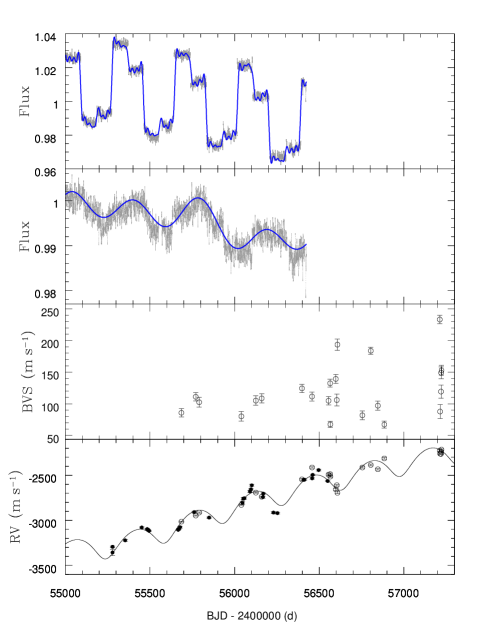
Figure 5: Top: The raw Kepler data of quarters Q2 – Q17 (grey curve). The blue curve is the sum of sine functions of periods found by Period04. Second from the top: The merged Kepler light curve of quarters Q2 – Q17 (grey curve) where one can see both long-period changes and short-period changes due to stellar oscillations. The blue curve is the sum of sine functions of three long periods found by Period04. Second from the bottom: Bisector velocity spans (BVS) measured from the average bisector values between flux levels of 0.1 – 0.3 and 0.7 – 0.9 of the continuum value, shown with corresponding error bars. Bottom: The RV variations of HD 175370 (TLS: filled circles, HERMES: open circles) shown for comparison.

Figure 6: Top: The frequency spectrum of bisector velocity spans. Second from the top: The frequency spectrum of Ca ii 8662 Å spectral line equivalent width measurements (solid line is the frequency spectrum for equivalent width measurements from 8661.0 to 8663.27 Å and dashed line from 8661.55 to 8662.8 Å). Second from the bottom: The frequency spectrum of the Kepler raw data without aligning individual quarters. Bottom: The frequency spectrum of merged Kepler data. See text for more details. A is the amplitude of the frequency spectra. The vertical line corresponds to the orbital period of the planetary candidate.

The period of 389.4 d is close to the orbital period of the Kepler satellite which is 372.5 d. In order to access whether this period is real, we have analysed raw light curves in the same way as above without aligning individual quarters. The raw Kepler data and the sum of sine functions of periods found by Period04 are shown in the top panel of Fig. 5 and the frequency spectrum is displayed in the second panel from the bottom of Fig. 6. We found a dominant period of 370 d which agrees very well with the orbital period of the Kepler satellite.

Every 3 months, the Kepler satellite was reoriented (rotated one-quarter turn) and then the light from each target star was collected by a new set of pixels on a different CCD. For precision photometry, this will introduce systematic errors. In addition, the orbital period of the Kepler satellite, 372.5 d, will also introduce systematic errors in the relative photometry. Therefore, finding a period in the Kepler data which is close to the orbital period of the satellite is suspicious. If one would like to use Kepler light curves to find periods of real physical processes close to the orbital period of the satellite, one would have to look at all K giants in the field and detrend them using a program like Sys-Rem (Mazeh, Tamuz & Zucker, 2007). Such systematic detrending would be useful for HD 175370, however, it is beyond the scope of this paper. Instead, we have looked at Kepler light curves of all 41 giant stars from our sample which we follow from Tautenburg and Mercator and which have corrected timeseries by the KASC Data Analysis Team. 76 per cent of targets show the dominant period of $390\pm 20~{}{\rm d}$, implying that the orbital period of the Kepler satellite can be really seen in the relative photometry of most of the giant stars. 7 per cent show the second dominant period of $379\pm 21~{}{\rm d}$. Finally, 17 per cent of targets show dominant periods which are clearly related to real physical processes and are not close to the orbital period of the satellite.

Both periods of 389.4 d and 370 d are also similar to the planetary orbital period of 349.5 d. We subtracted a linear trend from the photometric data shown in the second panel from the top of Fig. 5 and phase-folded them to the orbital period of the planet. The result is shown in Fig. 7, where the black dashed curve connects average values of the relative flux in bins of width 0.1 in phase. There is a modulation with an amplitude of about 0.0021 mag. The photometric time series cover nearly 3.5 planetary orbits. A careful look reveals that during the first two planetary orbits when photometric data were taken, photometric and RV variations agree quite well in phase, and only since the third orbit photometric and RV variations differ from each other (see Fig. 7). We have also phased the RV data to both photometric periods of 389.4 d and 370 d, and results are shown in Fig. 8. The solid curve represents a best fit allowing periastron epoch and semi-amplitude of the RV curve to vary and assuming a constant period and zero eccentricity. It can be seen that the RV data do not phase well with the photometric periods 370 and 389.4 d, having the scatter of RV residuals 63.6 and 75.4$\,\,\rm{m\,s^{-1}}$, respectively. Even though the above is not a proof that the RV period is unrelated to the photometric periods, there is no evidence to contradict this when taking into account that the Kepler photometry is suspicious for periods close to the orbital period of the satellite.

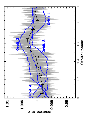
Figure 7: The Kepler light curve phase-folded to the orbital period of the planet (grey solid curve) and a running mean over 50 d (blue solid curve), where order of phase-folded orbits is shown. The black dashed curve shows the average values of the relative flux in bins of width 0.1 in phase. The error bars along the black dashed curve correspond to the standard deviation in each phase bin.

Figure 8: The RV data phased to the photometric periods of 370 d and 389.4 d. The solid curve represents a best fit allowing periastron epoch and semi-amplitude of the RV curve to vary and assuming a constant period and zero eccentricity.

In addition, a stellar rotation period is expected to be shorter than the period of the planetary candidate. With the measured projected rotational velocity of $v\,\sin i=6.11\pm 0.50\,\rm{km\,s^{-1}}$ and the radius of $R_{\ast}=23.5\pm 3.4\,R_{\odot}$ (RGB star) and $R_{\ast}=24.0\pm 3.2\,R_{\odot}$ (AGB star), the expected upper limit for the stellar rotation period is 194${}^{+48}_{-40}$ d and 199${}^{+46}_{-40}$ d, respectively. It is unlikely that the 349.5-d RV period represents the rotation period of the star. Assuming it did, this would result in a maximum projected rotational velocity of 3.4 $\pm$ 0.5 $\rm{km\,s^{-1}}$ (RGB star) and 3.5 $\pm$ 0.5 $\rm{km\,s^{-1}}$ (AGB star), or nearly a factor of two smaller than our measured $v\,\sin i$.

Furthermore, if the apparent sinusoidal photometric variations in the second panel from the top in Fig. 5 are due to cool spots, they cannot explain the observed RV variation. The amplitude of the photometric variations is $\sim$ 0.21 per cent. This results in a spot-induced RV amplitude of $\sim$ 11 m s^-1 (Saar & Donahue, 1997; Hatzes, 2002), or more than a factor of ten smaller than the observed $K$-amplitude.

5.2 Spectral line bisector analysis

Stellar rotational modulations of inhomogeneous surface features can create variable asymmetries in the spectral line profiles. The best way to describe this asymmetry is with the line bisector, which consists of the midpoints of horizontal line segments extending across the line profile. In a typical case, due to stellar granulation, the red wing of the stellar line is depressed, which causes the bisector to have a positive slope and curve to the right near the continuum level. We used the cross-correlation function (CCF) of the HermesDRS data reduction pipeline to calculate bisectors (see Fig. 9). Our CCF is typically based on $\sim$1650 spectral lines for each spectrum and this results in a very good accuracy for the bisector measurement. We are interested in relative and not absolute bisector measurements and according to Martínez Fiorenzano et al. (2005), the use of the average of many lines is appropriate for studying variations of line bisectors with time (see also e.g. Nowak et al. (2013)).

The best way to detect bisector changes is to calculate the bisector velocity span (BVS), which is the difference between bisectors at two different flux levels of a spectral line. As in Hatzes et al. (2015), we measured the BVS of the profile using the difference of the average bisector values between flux levels of 0.1 – 0.3 and 0.7 – 0.9 of the continuum value, therefore avoiding the spectral core and wing, where errors of the bisector measurements are larger. To estimate errors of bisectors we have used a formula of Martínez Fiorenzano et al. (2005), who modified the expression given by Gray (1983, 1988). Errors of our BVS measurements were then calculated by adding quadratically the errors for the top and bottom zones of the bisector measurements. Both BVS and their errors are listed in Table 1.

The BVS measurements are shown in the second panel from the bottom of Fig. 5. The BVS variations as a function of RV are shown in Fig. 10. Pearson’s correlation coefficient between RV and BVS variations amounts to -0.21 and the probability that they are uncorrelated is 0.29, indicating that they are not correlated. However, there are only a few BVS measurements around the minimum and maximum RV values and more data around these extremes would be useful.

We searched for periods in the BVS variations using the program Period04 (Lenz & Breger, 2005) and did not find any significant periods. The frequency spectrum is displayed in the top panel of Fig. 6.

Figure 9: Spectral line bisectors for all spectra of HD 175370 observed by the HERMES spectrograph, measured from the cross-correlation function based on $\sim$1650 spectral lines. BJD of the observation is shown on top of each bisector plot. Bisector velocity span errors are shown at lower right of each plot.

Figure 10: The BVS versus RV measurements for HD 175370 observed by the HERMES spectrograph.

5.3 Chromospheric activity

The equivalent width (EW) variations of the Ca ii H & K lines are often used as a chromospheric activity indicator because they are sensitive to stellar activity which in turn may affect the measured RV variations. In chromospherically active stars, the Ca ii H & K lines show a typical line core reversal (Pasquini, Pallavicini & Pakull, 1988). Mercator spectra of HD 175370 have a low S/N in the region of the Ca ii H & K lines and it is difficult to see if any emission features are present or not in the Ca ii H & K line cores.

Instead, we chose to measure chromospheric activity using the Ca ii triplet lines (Larson et al., 1993; Hatzes et al., 2003; Lee, Han & Park, 2013). Among the triplet lines, Ca ii 8662 Å  is not contaminated by atmospheric lines near the core. Additionally, Mercator spectra are contaminated by a light leak from the calibration fibre into the science fibre as displayed on the CCD in spectral regions containing bright calibration lines, but the region around the Ca ii 8662 Å line is free from the contamination. According to Larson et al. (1993), changes in the core flux of the line Ca ii 8662 Å are qualitatively related to the variations in the Ca ii H & K lines. We measured the EW at the central part of the Ca ii 8662 Å line from 8661.0 to 8663.27 Å and also from 8661.55 to 8662.8 Å and did not find any significant periodic changes. The frequency spectra are displayed in Fig. 6 in the second panel from the top. The variations of the Ca ii 8662 Å line are very small, which is typical for an inactive star.

6 Conclusions and discussion

Our spectral analysis of HD 175370 corresponds to a K2 III giant star. No carbon depletion or oxygen enhancement was detected in high-resolution spectra indicating that HD 175370 is a low-mass star, where hydrogen burning occurred in a radiative core, dominated by the proton-proton reactions so that the CNO cycle did not play a crucial role (Charbonnel et al., 1993). Based on the GBM code (Hekker et al., 2013), we deduce that HD 175370 is most likely a RGB or AGB star, and not a RC star.

We conclude that the RV variations of HD 175370 are caused by a low-mass stellar companion with an orbital period of $\sim 88$ years in a highly eccentric orbit and a possible planetary companion with an orbital period $P=349.5\pm 4.5~{}{\rm d}$, eccentricity $e=0.22\pm 0.10$, and a semi-amplitude $K=133\pm 25~{}{\rm m\,s^{-1}}$. Our interpretation of the RV changes in terms of a planet is supported by the lack of variability in the spectral line bisectors, Kepler light curve, and the lack of chromospheric activity corresponding to the orbital period of the planet. Furthermore, if 349.5 d were the rotation period of the star then this would result in a maximum projected stellar rotational velocity of 3.4 $\pm$ 0.5 $\rm{km\,s^{-1}}$ (RGB star) and 3.5 $\pm$ 0.5 $\rm{km\,s^{-1}}$ (AGB star), or nearly a factor of two smaller than our measured $v\,\sin i$.

However, even the lack of stellar variability in stellar activity indicators corresponding to the orbital period of the planet do not prove its existence. One caveat is 42 Dra which has been claimed to host a planetary companion (Döllinger et al., 2009). Our continued RV measurements of 42 Dra show that in the past three years the amplitude of the orbital motion decreased by a factor of four (Hatzes et al., in preparation). This casts serious doubts on the planet hypothesis for the RV variations. When the RV amplitude was high there were no variations in H$\alpha$, the spectral line bisectors, or in the Hipparcos photometry. In this case the standard tools for planet confirmation - the same ones that we use for HD 175370 - failed. We suggest that measurements of such standard activity indicators may not be sufficient and that long-term monitoring is essential in order to confirm planets around K-giant stars.

We note that we do not see any variations in the RV amplitude of the orbital motion due to HD 175370 b. The star 42 Dra showed coherent RV variations with a constant amplitude over three years. The RV variations in HD 175370 are constant for more than five years.

We found two periods in the Kepler light curves of 389.4 d and 370 d. Both of them are very close to the orbital period of the satellite, 372.5 d. We have shown that most of the Kepler giant stars from our sample show the dominant period of $390\pm 20~{}{\rm d}$, which agrees with the orbital period of the Kepler satellite within the 1-$\sigma$ error bars. We therefore believe that finding a period in the Kepler photometry which is close to the orbital period of the satellite is suspicious and should not be related to a real physical process unless one looks at all K giants in the field and detrends them systematically. Even though we cannot prove that the RV period is unrelated to the photometric periods, there is no evidence about the opposite. Continued RV monitoring of this system may help answer this uncertainty.

A possible explanation of the RV changes observed for HD 175370 could be an unknown envelope pulsation causing photometric and spurious Keplerian-like RV variations. Jorissen et al. (2016a, b) found among 13 low-metallicity giants three cases where small amplitude variations ($K$ ranging from 0.1 to 0.9 $\rm{km\,s^{-1}}$) with periods very close to 1 year are superimposed on a long-period Keplerian orbit. They do not give a conclusive answer on the origin of these variations, but leave an envelope pulsation as an option. In choosing a hypothesis based on a known phenomenon (exoplanets) as opposed to an unknown phenomenon (envelope oscillations) we chose the former until more evidence comes to light. In addition, we have shown that the photometric periods we have found in the Kepler light curves of HD 175370 are suspicious of being due to the orbital period of the satellite.

Oscillation modes dominate the short time-scale variations in the light curve and their amplitudes are at least ten times larger than the expected transit depth. It would therefore be difficult to detect any transit events in the light curve, which would constrain the orbital inclination.

HD 175370 is one of the few close binary systems to host a giant planetary candidate and thus may be important for understanding planet formation in binary systems. To date, only about six binary systems with separations less than 25 AU have been found to host giant planets (Morais & Correia, 2008; Ramm et al., 2009). With a binary orbital separation of 22 AU HD 175370 adds to this small list. HD 175370 is unique in that it has the largest binary eccentricity ($e$ = 0.88) of these binary systems hosting planetary candidates. At closest approach the primary-secondary separation is only a factor of 2.7 larger than the planet-star semi-major axis. However, we fixed the orbital period and eccentricity of the binary orbit to values obtained from varying these parameters separately and searched for a minimum in the residuals, and therefore the errors of both parameters are expected to be large, which also implies a large error on the orbital separation. We estimate that uncertainties of the period and eccentricity are $\sim$4000 d and $\sim$0.02, respectively, which implies that at closest approach the primary-secondary separation could be a factor of 3.5 larger than the planet-star semi-major axis. A dynamical study may place additional constraints on the age and future evolution of this system.

HD 175370 b is one of the first planetary candidates discovered around a Kepler giant star via the RV method. Unlike for other evolved giant stars with extrasolar planets detected by ground-based RV surveys, for HD 175370 we have high-quality Kepler photometry from which we can determine the stellar mass and radius in a more or less model independent way. The relative uncertainties of our derived stellar mass, stellar radius, and $\log g$ are 16, 14, and 1 per cent, respectively. HD 175370 is a relatively old star with an age of at least 5.4 Gyrs. More discoveries of planets around evolved giant stars can give us a better understanding of the mass dependence of planet formation and the evolution of planetary systems.

References

- Basu, Chaplin & Elsworth (2010) Basu S., Chaplin W.J., Elsworth Y., 2010, ApJ, 710, 1596
- Bedding et al. (2011) Bedding T. R. et al., 2011, Nature, 471, 608
- Butler et al. (1996) Butler R.P., Marcy G.W., Williams E., McCarthy C., Dosanjh P., Vogt S.S., 1996, PASP, 108, 500
- Cassan et al. (2012) Cassan A. et al., 2012, Nature, 481, 167
- Ciceri et al. (2015) Ciceri S., Lillo-Box J., Southworth J., Mancini L., Henning Th., Barrado D., 2015, A&A, 573L, 5
- Charbonnel et al. (1993) Charbonnel C., Meynet G., Maeder A., Schaller G., Schaerer D., 1993, A&AS, 101, 415
- De Ridder et al. (2009) De Ridder J. et al., 2009, Nature, 459, 398
- Döllinger et al. (2009) Döllinger M.P., Hatzes A.P., Pasquini L., Guenther E.W., Hartmann M., Girardi L., 2009, A&A, 499, 935
- Endl, Kürster & Els (2000) Endl M., Kürster M., Els S., 2000, A&A, 362, 585
- Famaey et al. (2005) Famaey B., Jorissen A., Luri X., Mayor M., Udry S., Dejonghe H., Turon C., 2005, A&A, 430, 165
- Frandsen et al. (2002) Frandsen S. et al., 2002, A&A, 394L, 5
- Frink et al. (2001) Frink S., Quirrenbach A., Fischer D., Röser S., Schilbach E., 2001, PASP, 113, 173
- Frink et al. (2002) Frink S., Mitchell D.S., Quirrenbach A., Fischer D.A., Marcy G.W., Butler R.P., 2002, ApJ, 576, 478
- García et al. (2011) García R. A. et al., 2011, MNRAS, 414, L6
- Gilliland et al. (2010) Gilliland R. L. et al., 2010, PASP, 122, 131
- Gray (1983) Gray D. F., 1983, PASP, 95, 252
- Gray (1988) Gray D. F., 1988, Lectures on Spectral-Line Analysis: F, G, and K Stars, Ontario Gray, Arva
- Guggenberger et al. (2016) Guggenberger E., Hekker S., Basu S., Bellinger E., 2016, MNRAS, 460, 4277
- Gustafsson et al. (2008) Gustafsson B., Edvardsson B., Eriksson K., Jørgensen U.G., Nordlund Å., Plez B., 2008, A&A, 486, 951
- Hatzes (2002) Hatzes A.P., 2002, AN, 323, 392
- Hatzes & Cochran (1993) Hatzes A.P., Cochran W.D., 1993, ApJ, 413, 339
- Hatzes & Cochran (1994) Hatzes A.P., Cochran W.D., 1994, ApJ, 432, 763
- Hatzes et al. (2003) Hatzes A.P., Cochran W.D., Endl M., McArthur B., Paulson D.B., Walker G.A.H., Campbell B., Yang S., 2003, ApJ, 599, 1383
- Hatzes et al. (2015) Hatzes A.P. et al., 2015, A&A, 580, 31
- Hekker et al. (2006) Hekker S., Reffert S., Quirrenbach A., Mitchell D.S., Fischer D.A., Marcy G.W., Butler R.P., 2006, A&A, 454, 943
- Hekker et al. (2008) Hekker S., Snellen I.A.G., Aerts C., Quirrenbach A., Reffert S., Mitchell D.S., 2008, A&A, 480, 215
- Hekker et al. (2010) Hekker S. et al., 2010, MNRAS, 402, 2049
- Hekker et al. (2013) Hekker S., Elsworth Y., Mosser B., Kallinger T., Basu S., Chaplin W. J., Stello D., 2013, A&A, 556, A59
- Horne & Baliunas (1986) Horne J.H., Baliunas S.L., 1986, ApJ, 302, 757
- Howard et al. (2012) Howard A. W. et al., 2012, ApJS, 201, 15
- Huber et al. (2010) Huber D. et al., 2010, ApJ, 723, 1607
- Huber et al. (2013) Huber D. et al., 2013, Science, 342, 331
- Høg et al. (2000) Høg E. et al., 2000, A&A, 355L, 27
- Johnson et al. (2010) Johnson J.A., Aller K.M., Howard A.W., Crepp J.R., 2010, PASP, 122, 905
- Jorissen et al. (2016a) Jorissen A., Hansen T., Van Eck S., Andersen J. et al., 2016a, A&A, 586, 159
- Jorissen et al. (2016b) Jorissen A., Van Eck S., Van Winckel H., Merle T. et al., 2016b, A&A, 586, 158
- Kennedy & Kenyon (2008) Kennedy G.M., Kenyon S.J., 2008, ApJ, 673, 502
- Kjeldsen & Bedding (1995) Kjeldsen H., Bedding T.R., 1995, A&A, 293, 87
- Koch et al. (2010) Koch D. G. et al., 2010, ApJ, 713L, 79
- Kurucz (1993) Kurucz R., 1993, ATLAS9 Stellar Atmosphere Programs and 2 grid, Kurucz CD-ROM No. 13, Smithsonian Astrophysical Observatory
- Kürster et al. (1997) Kürster M., Schmitt J.H.M.M., Cutispoto G., Dennerl K., 1997, A&A, 320, 831
- Larson et al. (1993) Larson A.M., Irwin A.W., Yang S.L.S., Goodenough C., Walker G.A.H., Walker A.R., Bohlender D.A., 1993, PASP, 105, 332
- Lebreton & Goupil (2014) Lebreton Y., Goupil M.J., 2014, A&A, 569, 21
- Lee, Han & Park (2013) Lee B.C., Han I., Park M.G., 2013, A&A, 549, 2
- Lehmann et al. (2011) Lehmann H. et al., 2011, A&A, 526, 124
- Lenz & Breger (2005) Lenz P., Breger M., 2005, CoAst, 146, 53
- Lillo-Box et al. (2014) Lillo-Box J. et al., 2014, A&A, 562, 109
- Lloyd (2011) Lloyd J. P., 2011, ApJ, 739L, 49
- Luck & Heiter (2007) Luck R.E., Heiter U., 2007, AJ, 133, 2464
- Mazeh, Tamuz & Zucker (2007) Mazeh T., Tamuz O., Zucker S., 2007, ASPC, 366, 119
- McArthur, Jefferys & McCartney (1994) McArthur B., Jefferys W., McCartney J., 1994, A&AS, 184, 2804
- McDonald, Zijlstra & Boyer (2012) McDonald I., Zijlstra A.A., Boyer M.L., 2012, MNRAS, 427, 343
- Martínez Fiorenzano et al. (2005) Martínez Fiorenzano A.F., Gratton R.G., Desidera S., Cosentino R., Endl M., 2005, A&A, 442, 775
- Morais & Correia (2008) Morais M.H.M., Correia A.C.M., 2008, A&A, 491, 899
- Mosser et al. (2014) Mosser B. et al., 2014, A&A, 572L, 5
- Nowak et al. (2013) Nowak G., Niedzielski A., Wolszczan A., Adamów M., Maciejewski G., 2013, ApJ, 770, 53
- Ortiz et al. (2015) Ortiz M. et al., 2015, A&A, 573L, 60
- Otor et al. (2016) Otor O.J. et al., 2016, ArXiv e-prints, arXiv:1608.03627
- Pasquini, Pallavicini & Pakull (1988) Pasquini L., Pallavicini R., Pakull M., 1988, A&A, 191, 253
- Pietrinferni et al. (2004) Pietrinferni A., Cassisi S., Salaris M., Castelli F., 2004, ApJ, 612, 168
- Quinn et al. (2015) Quinn S.N. et al., 2015, ApJ, 803, 49
- Ramm et al. (2009) Ramm D.J., Pourbaix D., Hearnshaw J.B., Komonjinda S., 2009, MNRAS, 394, 1695
- Raskin et al. (2011) Raskin G. et al., 2011, A&A, 526, A69
- Saar & Donahue (1997) Saar S.H., Donahue R.A., 1997, ApJ, 485, 319
- Scargle (1982) Scargle J. D., 1982, ApJ 263, 835
- Stello et al. (2013) Stello D. et al., 2013, ApJ, 765L, 41
- Tsymbal (1996) Tsymbal V., 1996, ASPC 108, 198
- Valenti, Butler & Marcy (1995) Valenti J.A., Butler R.P., Marcy G.W., 1995, PASP, 107, 966
- van Leeuwen (2007) van Leeuwen F., 2007, A&A, 474, 653
- Zechmeister & Kürster (2009) Zechmeister M., Kürster M., 2009, A&A, 496, 577