Polynomial-exponential decomposition from moments

Abstract

We analyze the decomposition problem of multivariate polynomial-exponential functions from their truncated series and present new algorithms to compute their decomposition.

Using the duality between polynomials and formal power series, we first show how the elements in the dual of an Artinian algebra correspond to polynomial-exponential functions. They are also the solutions of systems of partial differential equations with constant coefficients. We relate their representation to the inverse system of the isolated points of the characteristic variety.

Using the properties of Hankel operators, we establish a correspondence between polynomial-exponential series and Artinian Gorenstein algebras. We generalize Kronecker theorem to the multivariate case, by showing that the symbol of a Hankel operator of finite rank is a polynomial-exponential series and by connecting the rank of the Hankel operator with the decomposition of the symbol.

A generalization of Prony’s approach to multivariate decomposition problems is presented, exploiting eigenvector methods for solving polynomial equations. We show how to compute the frequencies and weights of a minimal polynomial-exponential decomposition, using the first coefficients of the series. A key ingredient of the approach is the flat extension criteria, which leads to a multivariate generalization of a rank condition for a Carathéodory-Fejér decomposition of multivariate Hankel matrices. A new algorithm is given to compute a basis of the Artinian Gorenstein algebra, based on a Gram-Schmidt orthogonalization process and to decompose polynomial-exponential series.

A general framework for the applications of this approach is described and illustrated in different problems. We provide Kronecker-type theorems for convolution operators, showing that a convolution operator (or a cross-correlation operator) is of finite rank, if and only if, its symbol is a polynomial-exponential function, and we relate its rank to the decomposition of its symbol. We also present Kronecker-type theorems for the reconstruction of measures as weighted sums of Dirac measures from moments and for the decomposition of polynomial-exponential functions from values. Finally, we describe an application of this method for the sparse interpolation of polylog functions from values.

AMS classification: 14Q20, 68W30, 47B35, 15B05

1 Introduction

Sensing is a classical technique, which is nowadays heavily used in many applications to transform continuous signals or functions into discrete data. In other contexts, in order to analyze physical phenomena or the evolution of our environments, large sequences of measurements can also be produced from sensors, cameras or scanners to discretize the problem.

An important challenge is then to recover the underlying structure of the observed phenomena, signal or function. This means to extract from the data, a structured or sparse representation of the function, which is easier to manipulate, to transmit or to analyze. Recovering this underlying structure can boil down to compute an explicit representation of the function in a given functional space. Usually, a “good” numerical approximation of the function as a linear combination of a set of basis functions is sufficient. The choice of the basis functions is very important from this perspective. It can lead to a representation, with many non-zero coefficients or a sparse representation with few coefficients, if the basis is well-suited. To illustrate this point, consider a linear function over a bounded interval of $\mathbb{R}$. It has a sparse representation in the monomial basis since it is represented by two coefficients. But its description as Fourier series involves an infinite sequence of (decreasing) Fourier coefficients.

This raises the questions of how to determine a good functional space, in which the functions we consider have a sparse representation, and how to compute such a decomposition, using a small (if not minimal) amount of information or measurements.

In the following, we consider a special reconstruction problem, which will allow us to answer these two questions in several other contexts. The functional space, in which we are going to compute sparse representations is the space of polynomial-exponential functions. The data that we use corresponds to the Taylor coefficients of these functions. Hereafter, we call them moments. They are for instance the Fourier coefficients of a signal or the values of a function sampled on a regular grid. It can also be High Order Statistical moments or cumulants, used in Signal Processing to perform blind identification [43]. Many other examples of reconstruction from moments can be found in Image Analysis, Computer Vision, Statistics …The reconstruction problem consists in computing a polynomial-exponential representation of the series from the (truncated) sequence of its moments. We will see that this problem allows us to recover sparse representations in several contexts.

With the multi-index notation: $\forall\alpha=(\alpha_{1},\ldots,\alpha_{n})\in\mathbb{N}^{n},\forall\mathbf{u}\in\mathbb{C}^{n}$, $\alpha!=\prod_{i=1}^{n}\alpha_{i}!$, $\mathbf{u}^{\alpha}=\prod_{i=1}^{n}u_{i}^{\alpha}$, $\mathbf{e}_{\xi}(\mathbf{y})=\sum_{\alpha\in\mathbb{N}^{n}}\frac{1}{\alpha!}\xi^{\alpha}\mathbf{y}^{\alpha}=e^{\langle\xi,\mathbf{{{y}}}\rangle}=e^{\xi_{1}y_{1}+\cdots+\xi_{n}y_{n}}$ for $\xi=(\xi_{1},\ldots,\xi_{n})\in\mathbb{C}^{n}$, and for $\mathbb{C}[[{\mathbf{y}}]]=\mathbb{C}[[y_{1},\ldots,y_{n}]]$ the ring of formal power series in $y_{1},\ldots,y_{n}$, this decomposition problem can be stated as follows.

Polynomial-exponential decomposition from moments: Given coefficients $\sigma_{\alpha}$ for $\alpha\in\mathbf{a}\subset\mathbb{N}^{n}$ of the series

$$\sigma(\mathbf{y})=\sum_{\alpha\in\mathbb{N}^{n}}\sigma_{\alpha}\frac{\mathbf{y}^{\alpha}}{\alpha!}\in\mathbb{C}[[{\mathbf{y}}]],$$

recover $r$ points $\mathbf{\xi}_{1},\ldots,\mathbf{\xi}_{r}\in\mathbb{C}^{n}$ and $r$ polynomial coefficients $\omega_{i}(\mathbf{y})\in\mathbb{C}[\mathbf{y}]$ such that

$$\sigma(\mathbf{y})=\sum_{i=1}^{r}\hskip 2.5pt\omega_{i}(\mathbf{y})\mathbf{e}_{{\xi_{i}}}(\mathbf{y}).$$ (1)

A function of the form (1) is called a polynomial-exponential function. We aim at recovering the minimal number $r$ of terms in the decomposition (1). Since only the coefficients $\sigma_{\alpha}$ for $\alpha\in\mathbf{a}$ are known, computing the decomposition (1) means that the coefficients of $\mathbf{y}^{\alpha}$ are the same in the series on both sides of the equality, for $\alpha\in\mathbf{a}$.

1.1 Prony’s method in one variable

One of the first work in this area is probably due to Gaspard-Clair-François-Marie Riche de Prony, mathematician and engineer of the École Nationale des Ponts et Chaussées. He was working on Hydraulics. To analyze the expansion of various gases, he proposed in [22] a method to fit a sum of exponentials at equally spaced data points in order to extend the model at intermediate points. More precisely, he was studying the following problem:

Given a function $h\in C^{\infty}(\mathbb{R})$ of the form

$$x\in\mathbb{R}\mapsto h(x)=\sum_{i=1}^{r}\hskip 2.5pt\omega_{i}\hskip 2.5pte^{f_{i}x}\in\mathbb{C}$$ (2)

where  $f_{1},\ldots,f_{r}\in\mathbb{C}$ are pairwise distinct, $\omega_{i}\in\mathbb{C}\setminus\{0\}$, the problem consists in recovering

• the distinct frequencies $f_{1},\ldots,f_{r}\in\mathbb{C}$,

• the coefficients $\omega_{i}\in\mathbb{C}\setminus\{0\}$,

Figure 1 shows an example of such a signal, which is the superposition of several “oscillations” with different frequencies.

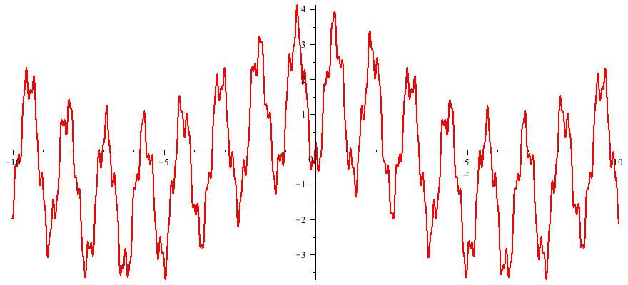
Figure 1: A superposition of oscillations with different frequencies

The approach proposed by G. de Prony can be reformulated into a truncated series reconstruction problem. By choosing an arithmetic progression of points in $\mathbb{R}$, for instance the integers $\mathbb{N}$, we can associate to $h$, the generating series:

$$\sigma_{h}(y)=\sum_{a\in\mathbb{N}}h(a)\frac{y^{a}}{a!}\in\mathbb{C}[[y]],$$

where $\mathbb{C}[[y]]$ is the ring of formal power series in the variable $y$. If $h$ is of the form (2), then

$$\sigma_{h}(y)=\sum_{i=1}^{r}\hskip 2.5pt\sum_{a\in\mathbb{N}}\omega_{i}\xi_{i}^{a}\frac{y^{a}}{a!}=\sum_{i=1}^{r}\omega_{i}e^{\xi_{i}y}$$ (3)

where $\xi_{i}=e^{f_{i}}$. Prony’s method consists in reconstructing the decomposition (3) from a small number of coefficients $h(a)$ for $a=0,\ldots,2r-1$. It performs as follows:

• From the values $h(a)$ for $a\in[0,\ldots,2r-1]$ , compute the polynomial

  $$p(x)=\prod_{i=1}^{r}(x-\xi_{i})=x^{r}-\sum_{j=0}^{r-1}p_{j}x^{j},$$

  which roots are $\xi_{i}=e^{f_{i}}$, $i=1,\ldots,r$ as follows. Since it satisfies the recurrence relations

  $$\forall j\in[0,\ldots,r-1],\hskip 28.45274pt\sum^{r-1}_{i=0}\sigma_{j+i}p_{i}-\sigma_{j+r}=-\sum_{i=1}^{r}w_{i}\xi_{i}^{j}p(\xi_{i})=0,$$

  it is the unique solution of the system:

  $$\left(\begin{array}[]{ccccc}\sigma_{0}&\sigma_{1}&\ldots&&\sigma_{r-1}\\ \sigma_{1}&&&{\mathinner{\mskip 1.0mu\raise 1.0pt\vbox{\kern 7.0pt\hbox{.}}\mskip 2.0mu\raise 4.0pt\hbox{.}\mskip 2.0mu\raise 7.0pt\hbox{.}\mskip 1.0mu}}&\\ \vdots&&{\mathinner{\mskip 1.0mu\raise 1.0pt\vbox{\kern 7.0pt\hbox{.}}\mskip 2.0mu\raise 4.0pt\hbox{.}\mskip 2.0mu\raise 7.0pt\hbox{.}\mskip 1.0mu}}&&\vdots\\ &{\mathinner{\mskip 1.0mu\raise 1.0pt\vbox{\kern 7.0pt\hbox{.}}\mskip 2.0mu\raise 4.0pt\hbox{.}\mskip 2.0mu\raise 7.0pt\hbox{.}\mskip 1.0mu}}&&&\\ \sigma_{r-1}&&\ldots&&\sigma_{2r-2}\end{array}\right)\left(\begin{array}[]{c}p_{0}\\ p_{1}\\ \vdots\\ \vdots\\ p_{r-1}\end{array}\right)=\left(\begin{array}[]{c}\sigma_{r}\\ \sigma_{r+1}\\ \vdots\\ \vdots\\ \sigma_{2r-1}\end{array}\right).$$ (4)

• Compute the roots $\xi_{1},\ldots,\xi_{r}$ of the polynomial $p(x)$.

• To determine the weight coefficients $w_{1},\ldots,w_{r}$, solve the following linear (Vandermonde) system:

  $$\left(\begin{array}[]{cccc}1&1&\ldots&1\\ \xi_{1}&\xi_{2}&\ldots&\xi_{r}\\ \vdots&\vdots&&\vdots\\ \xi_{1}^{r-1}&\xi_{2}^{r-1}&\ldots&\xi_{r}^{r-1}\end{array}\right)\left(\begin{array}[]{c}w_{1}\\ w_{2}\\ \vdots\\ w_{r}\end{array}\right)=\left(\begin{array}[]{c}h_{0}\\ h_{1}\\ \vdots\\ h_{r-1}\end{array}\right).$$

This approach can be improved by computing the roots $\xi_{1},\ldots,\xi_{r}$, directly as the generalized eigenvalues of a pencil of Hankel matrices. Namely, Equation (4) implies that

$$\overbrace{\left(\begin{array}[]{ccccc}\sigma_{0}&\sigma_{1}&\ldots&&\sigma_{r-1}\\ \sigma_{1}&&&{\mathinner{\mskip 1.0mu\raise 1.0pt\vbox{\kern 7.0pt\hbox{.}}\mskip 2.0mu\raise 4.0pt\hbox{.}\mskip 2.0mu\raise 7.0pt\hbox{.}\mskip 1.0mu}}&\\ \vdots&&{\mathinner{\mskip 1.0mu\raise 1.0pt\vbox{\kern 7.0pt\hbox{.}}\mskip 2.0mu\raise 4.0pt\hbox{.}\mskip 2.0mu\raise 7.0pt\hbox{.}\mskip 1.0mu}}&&\vdots\\ &{\mathinner{\mskip 1.0mu\raise 1.0pt\vbox{\kern 7.0pt\hbox{.}}\mskip 2.0mu\raise 4.0pt\hbox{.}\mskip 2.0mu\raise 7.0pt\hbox{.}\mskip 1.0mu}}&&&\\ \sigma_{r-1}&&\ldots&&\sigma_{2r-2}\end{array}\right)}^{H_{0}}\overbrace{\left(\begin{array}[]{ccccc}0&&&&p_{0}\\ 1&\ddots&&&p_{1}\\ &\ddots&\ddots&&\vdots\\ &&\ddots&0&\vdots\\ &&&1&p_{r-1}\end{array}\right)}^{M_{p}}=\overbrace{\left(\begin{array}[]{ccccc}\sigma_{1}&\sigma_{2}&\ldots&&\sigma_{r}\\ \sigma_{2}&&&{\mathinner{\mskip 1.0mu\raise 1.0pt\vbox{\kern 7.0pt\hbox{.}}\mskip 2.0mu\raise 4.0pt\hbox{.}\mskip 2.0mu\raise 7.0pt\hbox{.}\mskip 1.0mu}}&\\ \vdots&&{\mathinner{\mskip 1.0mu\raise 1.0pt\vbox{\kern 7.0pt\hbox{.}}\mskip 2.0mu\raise 4.0pt\hbox{.}\mskip 2.0mu\raise 7.0pt\hbox{.}\mskip 1.0mu}}&&\vdots\\ &{\mathinner{\mskip 1.0mu\raise 1.0pt\vbox{\kern 7.0pt\hbox{.}}\mskip 2.0mu\raise 4.0pt\hbox{.}\mskip 2.0mu\raise 7.0pt\hbox{.}\mskip 1.0mu}}&&&\\ \sigma_{r}&&\ldots&&\sigma_{2r-1}\end{array}\right)}^{H_{1}},$$ (5)

so that the generalized eigenvalues of the pencil $(H_{1},H_{0})$ are the eigenvalues of the companion matrix $M_{p}$ of $p(x)$, that is, its the roots $\xi_{1},\ldots,\xi_{r}$. This variant of Prony’s method is also called the pencil method in the literature.

For numerical improvement purposes, one can also chose an arithmetic progression  $\frac{a}{T}$  and $a\in[0,\ldots,2r-1]$, with $T\in\mathbb{R}^{+}$ of the same order of magnitude as the frequencies $f_{i}$. The roots of the polynomial $p$ are then $\xi_{i}=e^{\frac{f_{i}}{T}}$.

1.2 Related work

The approximation of functions by a linear combination of exponential functions appears in many contexts. It is the basis of Fourier analysis, where infinite series are involved in the decomposition of functions. The frequencies of these infinite sums of exponentials belong to an infinite grid on the imaginary axis in the complex plane.

An important problem is to represent or approximate a function by a sparse or finite sum of exponential terms, removing the constraints on the frequencies. This problem has a long history and many applications, in particular in signal processing [30], [55].

Many works have been developed in the one dimensional case, which refers to the well-known problem of parameter estimation for exponential sums. A first family of methods can be classified as Prony-type methods. To take into account the problem of noisy data, the recurrence relation is computed by minimization techniques [55][chap. 1]. Another type of methods is called Pencil-matrix [55][chap. 1]. Instead of computing a recurrence relation, the generalized eigenvalues of a pencil of Hankel matrices are computed. The survey paper [30] describes some of these minimization techniques implementing a variable projection algorithm and their applications in various domains, including antenna analysis with so-called MUSIC [67] or ESPRIT [63] methods. In [15], another approach based on conjugate-eigenvalue computation and low rank Hankel matrix approximation is proposed. The extension of this method in [58], called Approximate Prony Method, is using controlled perturbations. The problem of accurate reconstruction of sums of univariate polynomial-exponential functions associated to confluent Prony systems has been investigated in [8], where polynomial derivatives of Dirac measures correspond to polynomial weights.

The reconstruction problem has also been studied in the multi-dimensional case [5], [59], [39]. These methods are applicable for problems where the degree of the moments is high enough to recover the multivariate solutions from some projections in one dimension. Even more recently, techniques for solving polynomial equations, which rely on the computation of $H$-bases, have been exploited in this context [65].

The theory builds on the properties of Hankel matrices of finite rank, starting with a result due to [38] in the one variable case. This result states that there is an explicit correlation between polynomial-exponential series and Hankel operators of finite rank. The literature on Hankel operators is huge and mainly focus on one variable (see e.g. [54]). Kronecker’s result has been extended to several variables for multi-index sequences [60], [7], [4], for non-commutative variables [28], for integral cross-correlation operators [3]. In some cases as in [3], methods have been proposed to compute the rank in terms of the polynomial-exponential decomposition.

Hankel matrices are central in the theory of Padé approximants for functions of one variable. Here also a large literature exists for univariate Padé approximants: see e.g. [6] for approximation properties, [9] for numerical stability problems, [10], [69] for algorithmic aspects. The extension to multivariate functions is much less developed [60], [21].

This type of approaches is also used in sparse interpolation of black box polynomials. In the methods developed in [11], [71], further improved in [29], the sparse polynomial is evaluated at points of the form $(\omega_{1}^{k},\ldots,\omega_{n}^{k})$ where $\omega_{i}$ are prime numbers or primitive roots of unity of co-prime order. The sparse decomposition of the black box polynomial is computed from its values by a univariate Prony-like method.

Hankel matrices and their kernels also play an important role in error correcting codes. Reed-Solomon codes, obtained by evaluation of a polynomial at a set of points and convolution by a given polynomial, can be decoded from their syndrome sequence by computing the error locator polynomial [45][chap. 9]. This is a linear recurrence relation between the syndrome coefficients, which corresponds to a non-zero element in the kernel of a Hankel matrix. Berlekamp [12] and Massey [47] proposed an efficient algorithm to compute such polynomials. Sakata extended the approach to compute Gröbner bases of polynomials in the kernel of a multivariate Hankel matrix [64]. The computation of multivariate linear recurrence relations have been further investigated, e.g. in [27] and more recently in [14].

Computing polynomials in the kernel of Hankel matrices and their roots is also the basis of the method proposed by J.J. Sylvester [68] to decompose binary forms. This approach has been extended recently to the decomposition of multivariate symmetric and multi-symmetric tensors in [16], [13].

A completely different approach, known as compressive sensing, has been developed over the last decades to compute sparse decompositions of functions (see e.g. [17]). In this approach, a (large) dictionary of functions is chosen and a sparse combination with few non-zero coefficients is computed from some observations. This boils to find a sparse solution $X$ of an underdetermined linear system $Y=AX$. Such a solution, which minimizes the $\ell^{0}$ “norm” can be computed by $\ell^{1}$ minimization, under some hypothesis.

For the sparse reconstruction problem from a discrete set of frequencies, it is shown in [17] that the $\ell^{1}$ minimization provides a solution, for enough Fourier coefficients (at least $4r$) chosen at random. As shown in [57], this problem can also be solved by a Prony-like approach, using only $2r$ Fourier coefficients.

1.3 Contributions

In this paper, we analyze the problem of sparse decomposition of series from an algebraic point of view and propose new methods to compute such decompositions.

We exploit the duality between polynomials and formal power series. The formalism is strongly connected to the inverse systems introduced by F.S Macaulay [44]: evaluations at points correspond to exponential functions and the multiplication to derivation. This duality between polynomial equations and partial differential equations has been investigated previously, for instance in [61], [33], [46], [25], [36] [53], [52], [35]. We give here an explicit description of the elements in the dual of an Artinian algebra (Theorem 2.17), in terms of polynomial-exponential functions associated to the inverse system of the roots of the characteristic variety. This gives a new and complete characterization of the solutions of partial differential equations with constant coefficients for zero-dimensional partial differential systems (Theorem 2.18).

The sparse decomposition problem is tackled by studying the Hankel operators associated to the generating series. This approach has been exploited in many contexts: signal processing (see e.g. [55]), functional analysis (see e.g. [54]), but also in tensor decomposition problems [16], [13], or polynomial optimization [40]. Our algebraic formalism allows us to establish a correspondence between polynomial-exponential series and Artinian Gorenstein algebras using these Hankel operators.

A fundamental result on univariate Hankel operators of finite rank is Kronecker’s theorem [38]. Several works have already proposed multivariate generalization of Kronecker’s theorem, including methods to compute the rank of the Hankel operator from its symbol [60], [34], [31], [3], [4]. We prove a new multivariate generalization of Kronecker’s theorem (Theorem 3.1), showing that the symbol associated to a Hankel operator of finite rank is a polynomial-exponential series and describing its rank in terms of the polynomial weights. More precisely, we show that, as in the univariate case, the rank of the Hankel operator is simply the sum of the dimensions of the vector spaces spanned by all the derivatives of the polynomial weights of its symbol, represented as a polynomial-exponential series.

Exploiting classical eigenvector methods for solving polynomial equations, we show how to compute a polynomial-exponential decomposition, using the first coefficients of the generating series (Algorithms 3.1 and 3.2). In particular, we show how to recover the weights in the decomposition from the eigenspaces, for simple roots and multiple roots. Compared to methods used in [39] or [65], we need not solve polynomial equations deduced from elements in the kernel of the Hankel operator. We directly apply linear algebra operations on some truncated Hankel matrices to recover the decomposition. This allow us to use moments of lower degree compared for instance to methods proposed in [5], [59], [39].

This approach also leads to a multivariate generalization of Carathéodory-Fejér decomposition [18], which has been recently generalized to positive semidefinite multi-level block Toeplitz matrices in [70] and [4]. These results apply for simple roots or constant weights. Propositions 3.15 and 3.18 provide such a decomposition of Hankel matrices of a polynomial-exponential symbol in terms of the weights and generalized Vandermonde matrices, for simple and multiple roots.

To have a complete method for decomposing a polynomial-exponential series from its first moments using the proposed Algorithms 3.1 and 3.2, one needs to determine a basis of the Artinian Gorenstein algebra. A new algorithm is described to compute such a basis (Algorithm 4.1), which applies a Gram-Schmidt orthogonalization process and computes pairwise orthogonal polynomial bases. The method is connected to algorithms to compute linear recurrence relations of multi-index series, such as Berlekamp-Massey-Sakata algorithm [64], or [27], [14]. It proceeds inductively by projecting orthogonally new elements on the space spanned by the previous orthogonal polynomials, instead of computing the discrepancy of the new elements. Thus, it can compute more general basis of the ideal of recurrence relations, such as Border Bases [49], [51].

A key ingredient of the approach is the flat extension criteria. In Theorem 4.2, we provide such a criteria based on rank conditions, for the existence of a polynomial-exponential series extension. It generalizes results from [20], [42].

A general framework for the application of this approach based on generating series is described, extending the construction of [56] to the multivariate setting. We illustrate it in different problems, showing that several results in analysis are consequences of the algebraic multivariate Kronecker theorem (Theorem 3.1). In particular, we provide Kronecker-type theorems (Theorems 5.6, 5.7 and 5.9) for convolution operators (or cross-correlation operators), considered in [3], [4]. Theorem 3.1 implies that the rank of a convolution (or correlation) operator with a polynomial-exponential symbol is the sum of the dimensions of the space spanned by all the derivatives of the polynomial weights of the symbol. By Lemma 2.6, this gives a simple description of the output of the method proposed in [3] to compute the rank of convolution operators. We also deduce Kronecker-type theorems for the reconstruction of measures as weighted sums of Dirac measures from moments and the decomposition of polynomial-exponential functions from values. Finally, we describe a new approach for the sparse interpolation of polylog functions from values, with Kronecker-type results on their decomposition. Compared to previous approaches such as [11], [71], [29], we don’t project the problem in one dimension and recover sparse polylog terms from the multiplicity structure of the roots.

2 Duality and Hankel operators

In this section, we consider polynomials and series with coefficients in a field $\mathbb{K}$ of characteristic $0$. In the applications, we are going to take $\mathbb{K}=\mathbb{C}$ or $\mathbb{K}=\mathbb{R}$.

We are going to use the following notation: $\mathbb{K}[x_{1},\ldots,x_{n}]=\mathbb{K}[\mathbf{x}]=R$ is the ring of polynomials in the variables $x_{1},\ldots,x_{n}$ with coefficients in the field $\mathbb{K}$, $\mathbb{K}[[y_{1},\ldots,y_{n}]]=\mathbb{K}[[\mathbf{y}]]$ is the ring of formal power series in the variables $y_{1},\ldots,y_{n}$ with coefficients in $\mathbb{K}$. For a set $B\subset\mathbb{K}[\mathbf{x}]$, $B^{+}=\cup_{i=1}^{n}x_{i}B\cup B$, $\partial B=B^{+}\setminus B$. For $\alpha,\beta\in\mathbb{N}^{n}$, we say that $\alpha\ll\beta$ if $\alpha_{i}\leqslant\beta_{i}$ for $i=1,\ldots,n$.

2.1 Duality

In this section, we describe the natural isomorphism between the ring of formal power series and the dual of $R=\mathbb{K}[x_{1},\ldots,x_{n}]$. It is given by the following pairing:

$$\mathbb{K}[[y_{1},\ldots,y_{n}]]\times\mathbb{K}[x_{1},\ldots,x_{n}] \rightarrow \mathbb{K}$$

$$(\mathbf{y}^{\alpha},\mathbf{x}^{\beta}) \mapsto \left\langle\mathbf{y}^{\alpha}|\mathbf{x}^{\beta}\right\rangle=\left\{\begin{array}[]{ll}\alpha!&\operatorname{if}\alpha=\beta\\ 0&\operatorname{otherwise}.\end{array}\right.$$

Namely, if $\Lambda\in\operatorname{Hom}_{\mathbb{K}}(\mathbb{K}[\mathbf{x}],\mathbb{K})=R^{\ast}$ is an element of the dual of $\mathbb{K}[\mathbf{x}]$, it can be represented by the series:

$$\Lambda(\mathbf{y})=\sum_{\alpha\in\mathbb{N}^{n}}\Lambda(\mathbf{x}^{\alpha})\frac{\mathbf{y}^{\alpha}}{\alpha!}\in\mathbb{K}[[y_{1},\ldots,y_{n}]],$$ (7)

so that we have $\langle\Lambda(\mathbf{y})|\mathbf{x}^{\alpha}\rangle=\Lambda(\mathbf{x}^{\alpha})$. The map $\Lambda\in R^{\ast}\mapsto\sum_{\alpha\in\mathbb{N}^{n}}\Lambda(\mathbf{x}^{\alpha})\frac{\mathbf{y}^{\alpha}}{\alpha!}\in\mathbb{K}[[\mathbf{y}]]$ is an isomorphism and any series  $\sigma(\mathbf{y})=\sum_{\alpha\in\mathbb{N}^{n}}\sigma_{\alpha}\frac{\mathbf{y}^{\alpha}}{\alpha!}\in\mathbb{K}[[\mathbf{y}]]$ can be interpreted as a linear form

$$p=\sum_{\alpha\in A\subset\mathbb{N}^{n}}p_{\alpha}\mathbf{x}^{\alpha}\in\mathbb{K}[\mathbf{x}]\mapsto\langle\sigma\mid p\rangle=\sum_{\alpha\in A\subset\mathbb{N}^{n}}p_{\alpha}\sigma_{\alpha}.$$

Any linear form $\sigma\in R^{\ast}$ is uniquely defined by its coefficients $\sigma_{\alpha}=\langle\sigma\mid\mathbf{x}^{\alpha}\rangle$ for $\alpha\in\mathbb{N}^{n}$, which are called the moments of $\sigma$.

From now on, we identify the dual $\operatorname{Hom}_{\mathbb{K}}(\mathbb{K}[\mathbf{x}],\mathbb{K})$ with $\mathbb{K}[[\mathbf{y}]]$. Using this identification, the dual basis of the monomial basis $(\mathbf{x}^{\alpha})_{\alpha\in\mathbb{N}^{n}}$ is $\left(\frac{\mathbf{y}^{\alpha}}{\alpha!}\right)_{\alpha\in\mathbb{N}^{n}}$.

If $\mathbb{K}$ is a subfield of a field $\mathbb{L}$, we have the embedding $\mathbb{K}[[\mathbf{y}]]\hookrightarrow\mathbb{L}[[\mathbf{y}]]$, which allows to identify an element of $\mathbb{K}[\mathbf{x}]^{\ast}$ with an element of $\mathbb{L}[\mathbf{x}]^{\ast}$.

The truncation of an element $\sigma(\mathbf{y})=\sum_{\alpha\in\mathbb{N}^{n}}\sigma_{\alpha}\frac{\mathbf{y}^{\alpha}}{\alpha!}\in\mathbb{K}[[\mathbf{y}]]$ in degree $d$  is $\sum_{|\alpha|\leqslant d}\sigma_{\alpha}\frac{\mathbf{y}^{\alpha}}{\alpha!}$. It is denoted $\sigma(\mathbf{y})+((\mathbf{y}))^{d+1}$, that is, the class of $\sigma$ modulo the ideal  $(y_{1},\ldots,y_{n})^{d+1}\subset\mathbb{K}[[\mathbf{y}]]$.

For an ideal $I\subset R=\mathbb{K}[\mathbf{x}]$, we denote by $I^{\bot}\subset\mathbb{K}[[\mathbf{y}]]$ the space of linear forms $\sigma\in\mathbb{K}[[\mathbf{y}]]$, such that $\forall p\in I$, $\langle\sigma\mid p\rangle=0$. Similarly, for a vector space $D\subset\mathbb{K}[[\mathbf{y}]]$, we denoted by $D^{\bot}\subset\mathbb{K}[\mathbf{x}]$ the space of polynomials $p\in\mathbb{K}[\mathbf{x}]$, such that $\forall\sigma\in D$, $\langle\sigma\mid p\rangle=0$. If $D$ is closed for the $(\mathbf{y})$-adic topology, then $D^{\perp\perp}=D$ and if $I\subset\mathbb{K}[\mathbf{x}]$ is an ideal $I^{\perp}$, then $I^{\perp\perp}=I$.

The dual space $\operatorname{Hom}(\mathbb{K}[\mathbf{x}],\mathbb{K})\equiv\mathbb{K}[[\mathbf{y}]]$ has a natural structure of $\mathbb{K}[\mathbf{x}]$-module, defined as follows: $\forall\sigma(\mathbf{y})\in\mathbb{K}[[\mathbf{y}]],\forall p(\mathbf{x}),q(\mathbf{x})\in\mathbb{K}[\mathbf{x}]$,

$$\langle p(\mathbf{x})\star\sigma(\mathbf{y})\mid q(\mathbf{x})\rangle = \langle\sigma(\mathbf{y})\mid p(\mathbf{x})q(\mathbf{x})\rangle.$$

We check that $\forall\sigma\in\mathbb{K}[[\mathbf{y}]],\forall p,q\in\mathbb{K}[\mathbf{x}]$, $(pq)\star\sigma=p\star(q\star\sigma)$. See e.g. [25], [48] for more details.

For $p=\sum_{\beta}p_{\beta}\mathbf{x}^{\beta}\in\mathbb{K}[\mathbf{x}]$ and $\sigma=\sum_{\alpha\in\mathbb{N}^{n}}\sigma_{\alpha}\frac{\mathbf{y}^{\alpha}}{\alpha!}\in\mathbb{K}[[\mathbf{y}]]$, the series expansion of $p\star\sigma$ is $p\star\sigma=\sum_{\alpha\in\mathbb{N}^{n}}\rho_{\alpha}\frac{\mathbf{y}^{\alpha}}{\alpha!}\in\mathbb{K}[[\mathbf{y}]]$ with $\forall\alpha\in\mathbb{N}^{n},$

$$\rho_{\alpha}=\sum_{\beta}p_{\beta}\sigma_{\alpha+\beta}.$$

Identifying $\mathbb{K}[\mathbf{x}]$ with the set $\ell^{0}(\mathbb{K}^{\mathbb{N}^{n}})$ of sequences $p=(p_{\alpha})_{\alpha\in\mathbb{N}^{n}}$ of finite support (i.e. a finite number of non-zero terms), and $\mathbb{K}[[\mathbf{y}]]$ with the set of sequences $\sigma=(\sigma_{\alpha})_{\alpha\in\mathbb{N}^{n}}$, $p\star\sigma$ is the cross-correlation sequence of $p$ and $\sigma$.

For any $\sigma(\mathbf{y})\in\mathbb{K}[[\mathbf{y}]]$, the inner product associated to $\sigma(\mathbf{y})$ on $\mathbb{K}[\mathbf{x}]$ is defined as follows:

$$\mathbb{K}[\mathbf{x}]\times\mathbb{K}[\mathbf{x}] \rightarrow \mathbb{K}$$

$$(p(\mathbf{x}),q(\mathbf{x})) \mapsto \langle p(\mathbf{x}),q(\mathbf{x})\rangle_{\sigma}:=\langle\sigma(\mathbf{y})|p(\mathbf{x})q(\mathbf{x})\rangle.$$

2.1.1 Polynomial-Exponential series

Among the elements of $\operatorname{Hom}(\mathbb{K}[\mathbf{x}],\mathbb{K})\equiv\mathbb{K}[[\mathbf{y}]]$, we have the evaluations at points of $\mathbb{K}^{n}$:

Definition 2.1

The evaluation at a point $\xi=(\xi_{1},\ldots,\xi_{n})\in\mathbb{K}^{n}$ is:

$$\mathbf{e}_{{\xi}}:\mathbb{K}[x_{1},\ldots,x_{n}] \rightarrow \mathbb{K}$$

$$p(\mathbf{x}) \mapsto p(\xi)$$

It corresponds to the series:

$$\mathbf{e}_{{\xi}}(\mathbf{y}) = \sum_{\alpha\in\mathbb{N}^{n}}\xi^{\alpha}\frac{\mathbf{y}^{\alpha}}{\alpha!}=\hskip 2.5pte^{\xi_{1}y_{1}+\cdots+\xi_{n}y_{n}}=e^{\langle\xi,\mathbf{y}\rangle}.$$

Using this formalism, the series $\sigma(\mathbf{y})=\sum_{i=1}^{r}\omega_{i}\mathbf{e}_{\xi_{i}}(\mathbf{y})$ with $\omega_{i}\in\mathbb{K}$ can be interpreted as a linear combination of evaluations at the points $\xi_{i}$ with coefficients $\omega_{i}$, for $i=1,\ldots,r$. These series belong to the more general family of polynomial-exponential series, that we define now.

Definition 2.2

Let $\mathcal{PolExp}(y_{1},\ldots,y_{n})=\left\{\sigma=\sum_{i=1}^{r}\omega_{i}(\mathbf{y})\mathbf{e}_{\xi_{i}}(\mathbf{y})\in\mathbb{K}[[\mathbf{y}]]\mid\xi_{i}\in\mathbb{K}^{n},\omega_{i}(\mathbf{y})\in\mathbb{K}[\mathbf{y}]\right\}$ be the set of polynomial-exponential series. The polynomials $\omega_{i}(\mathbf{y})$ are called the weights of $\sigma$ and $\xi_{i}$ the frequencies.

Notice that the product of $\mathbf{y}^{\alpha}\mathbf{e}_{{\xi}}(\mathbf{y})$ with a monomial $\mathbf{x}^{\beta}\in\mathbb{C}[x_{1},\ldots,x_{n}]$ is given by

$$\left\langle\mathbf{y}^{\alpha}\mathbf{e}_{{\xi}}(\mathbf{y})|\mathbf{x}^{\beta}\right\rangle = \frac{\beta!}{(\beta-\alpha)!}\xi^{{}^{\beta-\alpha}}=\partial_{x_{1}}^{\alpha_{1}}\cdots\partial_{x_{n}}^{\alpha_{n}}(\mathbf{x}^{\beta})(\xi)\operatorname{if}\alpha_{i}\leqslant\beta_{i}\operatorname{for}i=1,\ldots,n$$

$$= 0\operatorname{otherwise}.$$

Therefore an element $\sigma=\sum_{i=1}^{r}\hskip 2.5pt\omega_{i}(\mathbf{y})\mathbf{e}_{{\xi_{i}}}(\mathbf{y})$ of $\mathcal{PolExp}(\mathbf{y})$ can also be seen as a sum of polynomial differential operators $\omega_{i}(\mathbf{\partial})$ “at” the points $\xi_{i}$, that we call infinitesimal operators: $\forall p\in\mathbb{K}[\mathbf{x}],\langle\sigma|p\rangle=\sum_{i=1}^{r}\hskip 2.5pt\omega_{i}(\mathbf{\partial})(p)(\xi)$.

2.1.2 Differential operators

An interesting property of the outer product defined on $\mathbb{K}[[\mathbf{y}]]$ is that polynomials act as differentials on the series:

Lemma 2.3

$\forall p\in\mathbb{K}[\mathbf{x}],\forall\sigma\in\mathbb{K}[[\mathbf{y}]]$, $p(\mathbf{x})\star\sigma(\mathbf{y})=p(\mathbf{\partial})(\sigma)$.

Proof.

We first prove the relation for $p=x_{i}$ ($i\in[1,n]$) and $\sigma=\mathbf{y}^{\alpha}$ ($\alpha\in\mathbb{N}^{n}$). Let $e_{i}=(0,\ldots,0,1,0,\ldots,0)$ be the exponent vector of $x_{i}$. $\forall\beta\in\mathbb{N}^{n}$ and $\forall i\in[1,n]$, we have

$$\left\langle x_{i}\star\mathbf{y}^{\alpha}|\mathbf{x}^{\beta}\right\rangle = \left\langle\mathbf{y}^{\alpha}|x_{i}\mathbf{x}^{\beta}\right\rangle=\hskip 10.00002pt\alpha!\hskip 10.00002pt\operatorname{if}\hskip 10.00002pt\alpha=\beta+e_{i}\hskip 10.00002pt\operatorname{and}\hskip 10.00002pt0\hskip 10.00002pt\operatorname{otherwise}$$

$$= \alpha_{i}\langle\mathbf{y}^{\alpha-e_{i}}|\mathbf{x}^{\beta}\rangle.$$

with the convention that $\mathbf{y}^{\alpha-e_{i}}=0$ if $\alpha_{i}=0$. This shows that $x_{i}\star\mathbf{y}^{\alpha}=\alpha_{i}\mathbf{y}^{\alpha-e_{i}}=\partial_{y_{i}}(\mathbf{y}^{\alpha})$. By transitivity and bilinearity of the product $\star$, we deduce that $\forall p\in\mathbb{K}[\mathbf{x}],\forall\sigma\in\mathbb{K}[[\mathbf{y}]]$, $p(\mathbf{x})\star\sigma(\mathbf{y})=p(\mathbf{\partial})(\sigma)$. ∎

This property can be useful to analyze the solution of partial differential equations. Let $p_{1}(\mathbf{\partial}),\ldots,p_{s}(\mathbf{\partial})\in\mathbb{K}[\partial_{1},\ldots,\partial_{n}]=\mathbb{K}[\mathbf{\partial}]$ be a set of partial differential polynomials with constant coefficients $\in\mathbb{K}$. The set of solutions $\sigma\in\mathbb{K}[[{\mathbf{y}}]]$ of the system

$$p_{1}(\mathbf{\partial})(\sigma)=0,\ldots,p_{s}(\mathbf{\partial})(\sigma)=0$$

is in correspondence with the elements $\sigma\in(p_{1},\ldots,p_{s})^{\bot}$, which satisfy $p_{i}\star\sigma=0$ for $i=1,\ldots,s$ (see Theorem 2.18). The variety $\mathcal{V}(p_{1},\ldots,p_{n})\subset\overline{\mathbb{K}}^{n}$ is called the characteristic variety and $I=(p_{1},\ldots,p_{n})$ the characteristic ideal of the system of partial differential equations.

Lemma 2.4

$\forall p\in\mathbb{K}[\mathbf{x}],\forall\omega\in\mathbb{K}[[\mathbf{y}]]$, $\xi\in\mathbb{K}^{n},p(\mathbf{x})\star(\omega(\mathbf{y})\mathbf{e}_{\xi}(\mathbf{y}))=p(\xi_{1}+\partial_{y_{1}},\ldots,\xi_{n}+\partial_{y_{n}})(\omega(\mathbf{y}))\mathbf{e}_{\xi}(\mathbf{y})$.

Proof.

By the previous lemma, $x_{i}\star(\omega(\mathbf{y})\mathbf{e}_{\xi}(\mathbf{y}))=\partial_{y_{i}}(\omega)(\mathbf{y})\mathbf{e}_{\xi}(\mathbf{y})+\xi_{i}\,\omega(\mathbf{y})\mathbf{e}_{\xi}(\mathbf{y})=(\xi_{i}+\partial_{y_{i}}$)$(\omega(\mathbf{y}))\mathbf{e}_{\xi}(\mathbf{y})$ for $i=1,\ldots,n$. We deduce that the relation is true for any polynomial $p\in\mathbb{K}[\mathbf{x}]$ by repeated multiplications by the variables and linear combination. ∎

Definition 2.5

For a subset $D\subset\mathbb{K}[[\mathbf{y}]]$, the inverse system generated by $D$ is the vector space spanned by the elements $p(\mathbf{x})\star\delta(\mathbf{y})$ for $\delta(\mathbf{y})\in D$, $p(\mathbf{x})\in\mathbb{K}[\mathbf{x}]$, that is, by the elements in $D$ and all their derivatives.

For $\omega\in\mathbb{K}[\mathbf{y}]$, we denote by ${\mu}(\omega)$ the dimension of the inverse system of $\omega$, generated by $\omega$ and all its derivatives $\mathbf{\partial}^{\alpha}(\omega)$, $\alpha\in\mathbb{N}^{n}$.

A simple way to compute this dimension is given in the next lemma:

Lemma 2.6

For $\omega\in\mathbb{K}[\mathbf{y}]$, $\mu(\omega)$ is the rank of the matrix $\Theta=(\theta_{\alpha,\beta})_{\alpha\in A,\beta\in B}$ where

$$\omega(\mathbf{y}+\mathbf{t})=\sum_{\alpha\in A\subset\mathbb{N}^{n},\beta\in B\subset\mathbb{N}^{n}}\theta_{\alpha,\beta}\,\mathbf{y}^{\alpha}\mathbf{t}^{\beta}$$

for some finite subsets $A,B$ of $\mathbb{N}^{n}$.

Proof.

The Taylor expansion of $\omega(\mathbf{y}+\mathbf{t})$ at $\mathbf{y}$ yields

$$\omega(\mathbf{y}+\mathbf{t})=\sum_{\beta\in B\subset\mathbb{N}^{n}}\mathbf{t}^{\beta}\frac{1}{\beta!}\mathbf{\partial}^{\beta}(\omega)(\mathbf{y})=\sum_{\beta\in B\subset\mathbb{N}^{n}}\mathbf{t}^{\beta}\sum_{\alpha\in A\subset\mathbb{N}}\theta_{\alpha,\beta}\,\mathbf{y}^{\alpha}.$$

This shows that the rank of the matrix $\Theta=(\theta_{\alpha,\beta})_{\alpha\in A,\beta\in B}$, that is, the rank of the vector space spanned by $\sum_{\alpha\in A\subset\mathbb{N}}\theta_{\alpha,\beta}\,\mathbf{y}^{\alpha}$ for $\beta\in B$ is the rank $\mu(\omega)$ of the vector space spanned by all the derivatives $\mathbf{\partial}^{\beta}(\omega)(\mathbf{y})$ of $\omega$. ∎

Lemma 2.7

The series $\mathbf{y}^{\alpha_{i,j}}\mathbf{e}_{{\xi_{i}}}(\mathbf{y})$ for $i=1,\ldots,r$ and $j=1,\ldots{\mu}_{i}$ with $\alpha_{i,1},\ldots,\alpha_{i,{\mu}_{i}}\in\mathbb{N}^{n}$ and $\xi_{i}\in\mathbb{K}^{n}$ pairwise distinct are linearly independent.

Proof.

Suppose that there exist $w_{i,j}\in\mathbb{K}$ such that $\sigma(\mathbf{y})=\sum_{i=1}^{r}\sum_{j=1}^{{\mu}_{i}}\omega_{i,j}\mathbf{y}^{\alpha_{i,j}}\mathbf{e}_{{\xi_{i}}}(\mathbf{y})=0$ and let $\omega_{i}(\mathbf{y})=\sum_{j=1}^{{\mu}_{i}}\omega_{i,j}\mathbf{y}^{\alpha_{i,j}}$. Then $\forall p\in\mathbb{K}[\mathbf{x}],p\star\sigma=0=\sum_{i=1}^{r}p(\xi_{i}+\mathbf{\partial})(\omega_{i})\mathbf{e}_{{\xi_{i}}}(\mathbf{y})$. If the weights $\omega_{i}(\mathbf{y})\in\mathbb{K}$ are of degree $0$, by choosing for $p$ an interpolation polynomial at one of the distinct points $\xi_{i}$, we deduce that $\omega_{i}=0$ for $i=1,\ldots,r$. If the weights $\omega_{i}(\mathbf{y})\in\mathbb{K}$ are degree $\geqslant 1$, by choosing $p=l(\mathbf{x})-l(\xi_{i})\in\mathbb{K}[\mathbf{x}]$ for a separating polynomial $l$ of degree $1$ ($l(\xi_{i})\neq l(\xi_{j})$ if $i\neq j$), we can reduce to a case where at least one of the non-zero weights has one degree less. By induction on the degree, we deduce that $\omega_{i}(\mathbf{y})=0$ for $i=1,\ldots,r$. This proves the linear independency of the series $\mathbf{y}^{\alpha_{i,j}}\mathbf{e}_{{\xi_{i}}}(\mathbf{y})$ for any $\alpha_{i,1},\ldots,\alpha_{i,{\mu}_{i}}\in\mathbb{N}^{n}$ and $\xi_{i}\in\mathbb{K}^{n}$ pairwise distinct. ∎

2.1.3 Z-transform and positive characteristic

In the identification (7) of $\operatorname{Hom}_{\mathbb{K}}(\mathbb{K}[\mathbf{x}],\mathbb{K})$ with the ring of power series in the variables $\mathbf{y}$, we can replace $\frac{\mathbf{y}^{\alpha}}{\alpha!}$  by $\mathbf{z}^{\alpha}$ where $\mathbf{z}=(z_{1},\ldots,z_{n})$ is a set of new variables, so that $\operatorname{Hom}_{\mathbb{K}}(\mathbb{K}[\mathbf{x}],\mathbb{K})$ is identified with $\mathbb{K}[[z_{1},\ldots,z_{n}]]=\mathbb{K}[[\mathbf{z}]]$. Any $\Lambda\in\operatorname{Hom}_{\mathbb{K}}(\mathbb{K}[\mathbf{x}],\mathbb{K})=R^{\ast}$ can be represented by the series:

$$\Lambda(\mathbf{y})=\sum_{\alpha\in\mathbb{N}^{n}}\Lambda(\mathbf{x}^{\alpha}){\mathbf{z}}^{\alpha}\in\mathbb{K}[[{\mathbf{z}}]]$$ (9)

where $(\mathbf{z}^{\alpha})_{\alpha\in\mathbb{N}^{n}}$ denotes the basis dual to the monomial basis $({\mathbf{x}}^{\alpha})_{\alpha\in\mathbb{N}^{n}}$ of $\mathbb{K}[{\mathbf{x}}]$. This corresponds to the Z-transform of the sequence $(\Lambda(\mathbf{x}^{\alpha}))_{\alpha\in\mathbb{N}^{n}}$ [1] or to the embedding in the ring of divided powers (${\mathbf{z}^{\alpha}}=\frac{\mathbf{y}^{\alpha}}{\alpha!}$) [23][Sec. A 2.4], [37][Appendix A]. It allows to extend the duality properties to any field $\mathbb{K}$, which is not of characteristic $0$.

The inverse transformation of the series $\sum_{\alpha\in\mathbb{N}^{n}}\sigma_{\alpha}{\mathbf{z}}^{\alpha}\in\mathbb{K}[[\mathbf{z}]]$ into the series $\sum_{\alpha\in\mathbb{N}^{n}}\sigma_{\alpha}\frac{\mathbf{y}^{\alpha}}{\alpha!}\in\mathbb{K}[[\mathbf{y}]]$ is known as the Borel transform [1].

For $\alpha,\beta\in\mathbb{N}^{n}$, we have$\begin{array}[]{lll}{\mathbf{x}}^{\alpha}\star{\mathbf{z}}^{\beta}&=&\left\{\begin{array}[]{ll}{\mathbf{z}}^{\beta-\alpha}&\operatorname{if}\beta-\alpha\in\mathbb{N}^{n}\\ 0&\operatorname{otherwise}\end{array}\right.\end{array}$so that $z_{i}$ plays the role of the inverse of $x_{i}$. This explains the terminology of inverse system, introduced in [44]. With this formalism, the variables $x_{1},\ldots,x_{n}$ act on the series in $\mathbb{K}[[\mathbf{z}]]$ as shift operators:

$$x_{i}\star\left(\sum_{\alpha\in\mathbb{N}^{n}}\sigma_{\alpha}{\mathbf{z}}^{\alpha}\right)=\sum_{\alpha\in\mathbb{N}^{n}}\sigma_{\alpha+e_{i}}{\mathbf{z}}^{\alpha}$$

where $e_{1},\ldots,e_{n}$ is the canonical basis of $\mathbb{N}^{n}$. Therefore, for any $p_{1},\ldots,p_{n}\in\mathbb{K}[\mathbf{x}]$, the system of equations

$$p_{1}\star\sigma=0,\ldots,p_{n}\star\sigma=0$$

corresponds to a system of difference equations on $\sigma\in\mathbb{K}[[\mathbf{z}]]$.

In this setting, the evaluation $\mathbf{e}_{\xi}$ at a point $\xi\in\mathbb{K}^{n}$ is represented in $\mathbb{K}[[\mathbf{z}]]$ by the rational fraction $\frac{1}{\prod_{j=1}^{n}(1-\xi_{j}z_{j})}$. The series $\mathbf{y}^{\beta}\mathbf{e}_{\xi}\in\mathbb{K}[[\mathbf{y}]]$ corresponds to the series of $\mathbb{K}[[\mathbf{z}]]$

$$\sum_{\alpha\in\mathbb{N}^{n}}\frac{(\alpha+\beta)!}{\alpha!}\xi^{\alpha}\mathbf{z}^{\alpha+\beta}=\beta!\mathbf{z}^{\beta}\sum_{\alpha\in\mathbb{N}^{n}}\binom{\alpha+\beta}{\beta}\xi^{\alpha}\mathbf{z}^{\alpha}=\frac{\beta!\,\mathbf{z}^{\beta}\hskip 2.5pt}{\prod_{j=1}^{n}(1-\xi_{j}z_{j})^{1+\beta_{j}}}.$$

The reconstruction of truncated series consists then in finding points $\mathbf{\xi}_{1},\ldots,\mathbf{\xi}_{r^{\prime}}\in\mathbb{K}^{n}$ and finite sets $A_{i}$ of coefficients $\omega_{i,\alpha}\in\mathbb{K}$ for $i=1,\ldots,r^{\prime}$ and $\alpha\in A_{i}$ such that

$$\sum_{\alpha\in\mathbb{N}^{n}}\sigma_{\alpha}{\mathbf{z}}^{\alpha}=\sum_{i=1}^{r^{\prime}}\sum_{\alpha\in A_{i}}\frac{\omega_{i,\alpha}\mathbf{z}^{\alpha}\hskip 2.5pt}{\prod_{i=1}^{n}(1-\xi_{i,j}z_{j})^{1+\alpha_{j}}}=\prod_{i=1}^{n}\bar{z}_{j}\sum_{i=1}^{r^{\prime}}\sum_{\alpha\in A_{i}}\frac{\omega_{i,\alpha}}{\prod_{i=1}^{n}(\bar{z}_{j}-\xi_{i,j})^{1+\alpha_{j}}}$$ (10)

where $\bar{z}_{j}=z_{j}^{-1}$.

In the univariate case, this reduces to computing polynomials $\omega(z),\delta(z)=\prod_{i=1}^{r^{\prime}}(1-\xi_{i}z)^{{\mu}_{i}}\in\mathbb{K}[z]$ with $\deg(\omega)<\deg(\delta)=\sum_{i}{\mu}_{i}=r$ such that

$$\sum_{k\in\mathbb{N}}\sigma_{k}z^{k}=\frac{w(z)}{\delta(z)}.$$

The decomposition can thus be computed from the Padé approximant of order $(r-1,r)$ of the sequence $(\sigma_{k})_{k\in\mathbb{N}}$ (see e.g. [69][chap. 5]).

Unfortunately, this representation in terms of Padé approximant does not extend so nicely to the multivariate case. The series $\sigma=\sum_{\alpha\in\mathbb{N}^{n}}\sigma_{\alpha}{\mathbf{z}}^{\alpha}$ with a decomposition of the form (10) correspond to the series $\sum_{\alpha\in\mathbb{N}^{n}}\sigma_{\alpha}{\mathbf{z}}^{-\alpha}$, which is rational of the form $\frac{\mathbf{z}^{\mathbf{1}}p(\mathbf{z})}{\prod q_{i}(z_{i})}$ with a splitable denominator where $\deg(q_{i})\geqslant 1$ are univariate polynomials (see e.g. [60], [7]). Though Padé approximants could be computed in this case by “separating” the variables (or by relaxing the constraints on the Padé approximants [21]), the rational fraction $\frac{\mathbf{z}^{\mathbf{1}}p(\mathbf{z})}{\prod q_{i}(z_{i})}$ is mixing the coordinates of the points  $\mathbf{\xi}_{1},\ldots,\mathbf{\xi}_{r^{\prime}}\in\mathbb{K}^{n}$ and the weights $\omega_{i,\alpha}$.

As the duality between multiplication and differential operators is less natural in $\mathbb{K}[[\mathbf{z}]]$, we will use hereafter the identification (7) of $R^{*}$ with $\mathbb{K}[[\mathbf{y}]]$, when $\mathbb{K}$ is of characteristic $0$.

2.2 Hankel operators

The product $\star$ allows us to define a Hankel operator as a multiplication operator by a dual element $\in\mathbb{K}[[\mathbf{y}]]$:

Definition 2.8

The Hankel operator associated to an element $\sigma(\mathbf{y})\in\mathbb{C}[[\mathbf{y}]]$ is

$$H_{\sigma}:\mathbb{K}[\mathbf{x}] \rightarrow \mathbb{K}[[\mathbf{y}]]$$

$$p(\mathbf{x}) \mapsto p(\mathbf{x})\star\sigma(\mathbf{y}).$$

Its kernel is denoted $I_{\sigma}=\ker H_{\sigma}$. The series $\sigma=\sum_{\alpha\in\mathbb{N}^{n}}\sigma_{\alpha}\frac{\mathbf{y}^{\alpha}}{\alpha!}=H_{\sigma}(1)\in\mathbb{K}[[\mathbf{y}]]$ is called the symbol of $H_{\sigma}$.

Definition 2.9

The rank of an element $\sigma\in\mathbb{K}[[\mathbf{y}]]$ is the rank of the Hankel operator $H_{\sigma}=r$.

Definition 2.10

The variety $\mathcal{V}_{\overline{\mathbb{K}}}(I_{\sigma})$ is called the characteristic variety of $\sigma$.

The Hankel operator can also be interpreted as an operator on sequences:

$$H_{\sigma}:\ell^{0}(\mathbb{K}^{\mathbb{N}^{n}}) \rightarrow \mathbb{K}^{\mathbb{N}^{n}}$$

$$p=(p_{\beta})_{\beta\in B\subset\mathbb{N}^{n}} \mapsto p\star\sigma=\left(\sum_{\beta\in B}p_{\beta}\sigma_{\alpha+\beta}\right)_{\alpha\in\mathbb{N}^{n}}$$

where $\ell^{0}(\mathbb{K}^{\mathbb{N}^{n}})$ is the set of sequences $\in\mathbb{K}^{\mathbb{N}^{n}}$ with a finite support. This definition applies for a field $\mathbb{K}$ of any characteristic. The operator $H_{\sigma}$ can also be interpreted, via the Z-transform of the sequence $p\star\sigma$ (see Section 2.1.3), as the Hankel operator

$$H_{\sigma}:\mathbb{K}[\mathbf{x}] \rightarrow \mathbb{K}[[\mathbf{z}]]$$

$$p=\sum_{\beta\in B}p_{\beta}\mathbf{x}^{\beta} \mapsto p\star\sigma=\sum_{\alpha\in\mathbb{N}^{n}}\left(\sum_{\beta\in B}p_{\beta}\sigma_{\alpha+\beta}\right)\mathbf{z}^{\alpha}.$$

As $\forall p,q\in\mathbb{K}[\mathbf{x}]$,  $pq\star\sigma=p\star(q\star\sigma)$, we easily check that $I_{\sigma}=\ker H_{\sigma}$ is an ideal of $\mathbb{K}[\mathbf{x}]$ and that $\mathcal{A}_{\sigma}=\mathbb{K}[\mathbf{x}]/I_{\sigma}$ is an algebra.

Since  $\forall p(\mathbf{x}),q(\mathbf{x})\in\mathbb{K}[\mathbf{x}]$, $\langle p(\mathbf{x})+I_{\sigma},q(\mathbf{x})+I_{\sigma}\rangle_{\sigma}=\langle p(\mathbf{x}),q(\mathbf{x})\rangle_{\sigma}$, we see that  $\langle\cdot,\cdot\rangle_{\sigma}$ induces an inner product on $\mathcal{A}_{\sigma}$.

Given a sequence $\sigma=(\sigma_{\alpha})_{\alpha\in\mathbb{N}^{n}}\in\mathbb{K}^{\mathbb{N}^{n}}$, the kernel of $H_{\sigma}$ is the set of polynomials $p=\sum_{\beta\in B}p_{\beta}\mathbf{x}^{\beta}$ such that $\sum_{\beta\in B}p_{\beta}\sigma_{\alpha+\beta}=0$ for all $\alpha\in\mathbb{N}^{n}$. This kernel is also called the set of linear recurrence relations of the sequence $\sigma=(\sigma_{\alpha})_{\alpha\in\mathbb{N}^{n}}$.

Example 2.11

If $\sigma=\mathbf{e}_{\xi}\in\mathbb{K}[[\mathbf{y}]]$ is the evaluation at a point $\xi\in\mathbb{K}^{n}$, then $H_{\mathbf{e}_{\xi}}:p\in\mathbb{K}[\mathbf{x}]\mapsto p(\xi)\mathbf{e}_{\xi}(\mathbf{y})\in\mathbb{K}[[\mathbf{y}]]$. We easily check that $\operatorname{rank}H_{\mathbf{e}_{\xi}}=1$ since the image of $H_{\mathbf{e}_{\xi}}$ is spanned by $\mathbf{e}_{\xi}(\mathbf{y})$ and that $I_{\mathbf{e}_{\xi}}=(x_{1}-\xi_{1},\ldots,x_{n}-\xi_{n})$.

If $\sigma=\sum_{i=1}^{r}\hskip 2.5pt\omega_{i}(\mathbf{y})\mathbf{e}_{{\xi_{i}}}(\mathbf{y})$ then, by Lemma 2.3, the kernel $I_{\sigma}$ is the set of polynomials $p\in\mathbb{K}[\mathbf{x}]$ such that $\forall q\in\mathbb{K}[\mathbf{x}]$, $p$ is a solution of the following partial differential equation:

$$\sum_{i=1}^{r}\hskip 2.5pt\omega_{i}(\mathbf{\partial})(pq)(\xi_{i})=0.$$

Remark 2.12

The matrix of the operator $H_{\sigma}$ in the basis $(\mathbf{x}^{\alpha})_{\alpha\in\mathbb{N}^{n}}$ and its dual basis $\left(\frac{\mathbf{y}^{\alpha}}{\alpha!}\right)_{\alpha\in\mathbb{N}^{n}}$ is

$${}[H_{\sigma}] = (\sigma_{\alpha+\beta})_{\alpha,\beta\in\mathbb{N}^{n}}=(\langle\sigma|\mathbf{x}^{\alpha+\beta}\rangle)_{\alpha,\beta\in\mathbb{N}^{n}}.$$

In the case $n=1$, the coefficients of $[H_{\sigma}]$ depends only on the sum of the indices indexing the rows and columns, which explains why it is are called a Hankel operator.

2.2.1 Truncated Hankel operators

In the sparse reconstruction problem, we are dealing with truncated series with known coefficients $\sigma_{\alpha}$ for $\alpha$ in a subset $\mathbf{a}$ of $\mathbb{N}^{n}$. This leads to the definition of truncated Hankel operators.

Definition 2.13

For two vector spaces $V,V^{\prime}\subset\mathbb{K}[\mathbf{x}]$ and  $\sigma\in\langle V\cdot V^{\prime}\rangle^{\ast}=\langle v\cdot v^{\prime}\mid v\in V,v^{\prime}\in V^{\prime}\rangle^{\ast}\subset\mathbb{K}[[\mathbf{y}]]$, we denote by $H_{\sigma}^{V,V^{\prime}}$ the following map:

$$H^{V,V^{\prime}}_{\sigma}:V \rightarrow V^{\prime\ast}=\hom_{\mathbb{K}}(V^{\prime},\mathbb{K})$$

$$p(\mathbf{x}) \mapsto p(\mathbf{x})\star\sigma(\mathbf{y})_{|V^{\prime}}.$$

It is called the truncated Hankel operator on $(V,V^{\prime})$.

When $V^{\prime}=V$, the truncated Hankel operator is also denoted $H_{\sigma}^{V}$. When $V$ (resp. $V^{\prime}$) is the vector space of polynomials of degree $\leqslant d\in\mathbb{N}$ (resp. $\leqslant d^{\prime}\in\mathbb{N}$), the truncated operator is denoted $H_{\sigma}^{d,d^{\prime}}$. If $B=\{b_{1},\ldots,b_{r}\}$ (resp. $B^{\prime}=\{b_{1}^{\prime},\ldots,b_{r}^{\prime}\}$) is a basis of $V$ (resp. $V^{\prime}$), then the matrix of the operator $H_{\sigma}^{V,V^{\prime}}$ in $B$ and the dual basis of $B^{\prime}$ is

$$[H_{\sigma}^{B,B^{\prime}}]=(\langle\sigma|b_{j}b_{i}^{\prime}\rangle)_{1\leqslant i,j\leqslant r}.$$

If $B=\mathbf{x}^{\mathbf{b}}$ and $B^{\prime}=\mathbf{x}^{\mathbf{b}^{\prime}}$ are monomial sets, we obtain the so-called truncated moment matrix of $\sigma$:

$${}[H_{\sigma}^{B,B^{\prime}}] = (\sigma_{\beta+\beta^{\prime}})_{\beta^{\prime}\in\mathbf{b}^{\prime},\beta\in\mathbf{b}}.$$

When $n=1$, this matrix is a classical Hankel matrix, which entries depend only on the sum of the indices of the rows and columns. When $n\geqslant 2$, we have a similar family of structured matrices whose rows and columns are indexed by exponents in $\mathbb{N}^{n}$ and whose entries depends on the sum of the row and column indices. These structured matrices called quasi-Hankel matrices have been studied for instance in [50].

2.3 Artinian algebra

In this section, we recall the properties of Artinian algebras. Let $I\subset\mathbb{K}[\mathbf{x}]$ be an ideal and let  $\mathcal{A}=\mathbb{K}[\mathbf{x}]/I$ be the associated quotient algebra.

Definition 2.14

The quotient algebra $\mathcal{A}$ is Artinian if $\dim_{\mathbb{K}}(\mathcal{A})<\infty.$

Notice that if $\mathbb{K}$ is a subfield of a field $\mathbb{L}$, we denote by $\mathcal{A}_{\mathbb{L}}=\mathbb{L}[\mathbf{x}]/I_{\mathbb{L}}=\mathcal{A}\otimes\mathbb{L}$ where $I_{\mathbb{L}}=I\otimes\mathbb{L}$ is the ideal of $\mathbb{L}[\mathbf{x}]$ generated by the elements in $I$. As the dimension does not change by extension of the scalars, we have $\dim_{\mathbb{K}}(\mathbb{K}[\mathbf{x}]/I)=\dim_{\mathbb{L}}(\mathbb{L}[\mathbf{x}]/I_{\mathbb{L}})=\dim_{\mathbb{L}}(\mathcal{A}_{\mathbb{L}})$. In particular, $\mathcal{A}$ is Artinian if and only if $\mathcal{A}_{\bar{\mathbb{K}}}$ is Artinian, where $\bar{\mathbb{K}}$ is the algebraic closure. For the sake of simplicity, we are going to assume hereafter that $\mathbb{K}$ is algebraically closed.

A classical result  states that the quotient algebra $\mathcal{A}=\mathbb{K}[\mathbf{x}]/I$ is finite dimensional, i.e. Artinian , if and only if, $\mathcal{V}_{\bar{\mathbb{K}}}(I)$ is finite, that is, $I$ defines a finite number of (isolated) points in $\bar{\mathbb{K}}^{n}$ (see e.g. [19][Theorem 6] or [24][Theorem 4.3]). Moreover, we have the following structure theorem (see [24][Theorem 4.9]):

Theorem 2.15

Let $\mathcal{A}=\mathbb{K}[\mathbf{x}]/I$ be an Artinian algebra of dimension $r$ defined by an ideal $I$. Then we have a decomposition into a direct sum of subalgebras

$$\mathcal{A}=\mathcal{A}_{\xi_{1}}\oplus\cdots\oplus\mathcal{A}_{\xi_{r^{\prime}}}$$ (11)

where

• $\mathcal{V}(I)=\{\xi_{1},\ldots,\xi_{r^{\prime}}\}\subset\bar{\mathbb{K}}^{n}$ with $r^{\prime}\leqslant r$.

• $I=Q_{1}\cap\cdots\cap Q_{r^{\prime}}$ is a minimal primary decomposition of $I$ where $Q_{i}$ is $\mathbf{m}_{\xi_{i}}$-primary with $\mathbf{m}_{\xi_{i}}=(x_{1}-\xi_{i,1},\ldots,x_{n}-\xi_{i,n})$.

• $\mathcal{A}_{\xi_{i}}\equiv\mathbb{K}[\mathbf{x}]/Q_{i}$ and $\mathcal{A}_{\xi_{i}}\cdot\mathcal{A}_{\xi_{j}}\equiv 0$ if $i\neq j$.

We check that $\mathcal{A}$ localized at $\mathbf{m}_{\xi_{i}}$ is the local algebra $\mathcal{A}_{\xi_{i}}$. The dimension of $\mathcal{A}_{\xi_{i}}$ is the multiplicity of the point $\xi_{i}$ in $\mathcal{V}(I)$.

The projection of $1$ on the sub-algebras $\mathcal{A}_{\xi_{i}}$ as

$$1\equiv{\mathbf{u}}_{\xi_{1}}+\cdots+\mathbf{u}_{\xi_{r^{\prime}}}$$

with ${\mathbf{u}}_{\xi_{i}}\in\mathcal{A}_{\xi_{i}}$ yields the so-called idempotents $\mathbf{u}_{\xi_{i}}$ associated to the roots $\xi_{i}$. By construction, they satisfy the following relations in $\mathcal{A}$, which characterize them:

• $1\equiv{\mathbf{u}}_{\xi_{1}}+\cdots+\mathbf{u}_{\xi_{r^{\prime}}}$,

• ${\mathbf{u}}_{\xi_{i}}^{2}\equiv{\mathbf{u}}_{\xi_{i}}$ for $i=1,\ldots,r^{\prime}$,

• ${\mathbf{u}}_{\xi_{i}}{\mathbf{u}}_{\xi_{j}}\equiv 0$ for $1\leqslant i,j\leqslant r^{\prime}$ and $i\neq j$.

The dual $\mathcal{A}^{\ast}=\operatorname{Hom}_{\mathbb{K}}(\mathcal{A},\mathbb{K})$ of $\mathcal{A}=\mathbb{K}[\mathbf{x}]/I$ is naturally identified with the subspace

$$I^{\bot}=\{\Lambda\in\mathbb{K}[\mathbf{x}]^{\ast}=\mathbb{K}[[\mathbf{y}]]\mid\forall p\in I,\Lambda(p)=0\}$$

of $\mathbb{K}[\mathbf{x}]^{\ast}=\mathbb{K}[[\mathbf{y}]]$. As $I$ is stable by multiplication by the variables $x_{i}$, the orthogonal subspace $I^{\bot}=\mathcal{A}^{\ast}$ is stable by the derivations $\frac{d}{\operatorname{dy}_{i}}$: $\forall\Lambda\in I^{\perp}\subset\mathbb{K}[[\mathbf{y}]]$, $\forall\,i=1\ldots n,$ $\frac{d}{\operatorname{dy}_{i}}(\Lambda)\in I^{\perp}$. In the case of a primary ideal, the orthogonal subspace has a simple form [44], [25], [48]:

Proposition 2.16

Let $Q$ be a primary ideal for the maximal ideal $\mathfrak{m}_{\xi}$ of the point $\xi\in\mathbb{K}^{n}$ and let $\mathcal{A}_{\xi}=\mathbb{K}[\mathbf{x}]/Q$. Then

$$Q^{\bot}=\mathcal{A}_{\xi}^{\ast}=D_{\xi}(Q)\cdot\mathbf{e}_{\xi}(\mathbf{y}),$$

where $D_{\xi}(Q)\subset\mathbb{K}[\mathbf{y}]$ is the set of polynomials $\omega(\mathbf{y})\in\mathbb{K}[\mathbf{y}]$ such that $\forall q\in Q$, $\omega(\mathbf{\partial})(q)(\xi)=0$.

The vector space $D_{\xi}(Q)\subset\mathbb{K}[\mathbf{y}]$ is called the inverse system of $Q$. As $Q$ is an ideal, $Q^{\bot}=D_{\xi}(Q)\cdot\mathbf{e}_{\xi}(\mathbf{y})$ is stable by the derivations $\frac{d}{\operatorname{dy}_{i}}$, and so is $D_{\xi}(Q)$.

If $I=Q_{1}\cap\cdots\cap Q_{r^{\prime}}$ is a minimal primary decomposition of the zero-dimensional ideal $I\subset\mathbb{K}[\mathbf{x}]$ with $Q_{i}$ $\mathbf{m}_{\xi_{i}}$-primary, then the decomposition (11) implies that

$$\mathcal{A}^{\ast}=I^{\bot}=Q_{1}^{\bot}\oplus\cdots\oplus Q_{r^{\prime}}^{\bot}=\mathcal{A}_{\xi_{1}}^{\ast}\oplus\cdots\oplus\mathcal{A}_{\xi_{r^{\prime}}}^{\ast}$$

since $Q_{i}^{\bot}\cap Q_{j}^{\bot}=(Q_{i}+Q_{j})^{\bot}=(1)^{\bot}=\{0\}$ for $i\neq j$. The elements of $\mathcal{A}_{\xi_{i}}^{\ast}$ are the elements $\Lambda\in\mathcal{A}^{\ast}=I^{\bot}$ such that $\forall a_{j}\in\mathcal{A}_{j}$ $j\neq i$, $\lambda(a_{j})=0$. Any element $\Lambda\in\mathcal{A}^{\ast}$ decomposes as

$$\Lambda={\mathbf{u}}_{\xi_{1}}\star\Lambda+\cdots+{\mathbf{u}}_{\xi_{r^{\prime}}}\star\Lambda.$$ (12)

As we have ${\mathbf{u}}_{\xi_{i}}\star\Lambda(\mathcal{A}_{\xi_{j}})=\Lambda({\mathbf{u}}_{\xi_{i}}\mathcal{A}_{\xi_{j}})=0$ for $i\neq j$, we deduce that ${\mathbf{u}}_{\xi_{i}}\star\Lambda\in\mathcal{A}_{\xi_{i}}^{\ast}=Q_{i}^{\bot}$

By Proposition 2.16, $Q_{i}^{\perp}=D_{i}\mathbf{e}_{\xi}(\mathbf{y})$ where $D_{i}=D_{\xi_{i}}(Q_{i})$ is the inverse system of $Q_{i}$. A basis of $D_{i}$ can be computed (efficiently) from $\xi_{i}$ and the generators of the ideal $I$ (see e.g. [48] for more details).

From the decomposition (12) and Proposition 2.16, we deduce the following result:

Theorem 2.17

Assume that $\mathbb{K}$ is algebraically closed. Let $\mathcal{A}$ be an Artinian algebra of dimension $r$ with $\mathcal{V}(I)=\{\xi_{1},\ldots,\xi_{r^{\prime}}\}\subset\mathbb{K}^{n}$. Let $D_{i}=D_{\xi_{i}}(I)\subset\mathbb{K}[\mathbf{y}]$ be the vector space of differential polynomials $\omega(\mathbf{y})\in\mathbb{K}[\mathbf{y}]$ such that $\forall p\in I,\omega(\mathbf{\partial})(p)(\xi_{i})=0$. Then $D_{i}$ is stable by the derivations $\frac{d}{\operatorname{dy}_{i}}$, $i=1,\ldots,n$. It is of dimension ${\mu}_{i}$ with $\sum_{i=1}^{r^{\prime}}{\mu}_{i}=r$. Any element $\Lambda$ of $\mathcal{A}^{\ast}$ has a unique decomposition of the form

$$\Lambda(\mathbf{y})=\sum_{i=1}^{r^{\prime}}\omega_{i}(\mathbf{y})\mathbf{e}_{\xi_{i}}(\mathbf{y}),$$ (13)

with $\omega_{i}(\mathbf{y})\in D_{i}\subset\mathbb{K}[\mathbf{y}]$, which is uniquely determined by values $\langle\Lambda|b_{i}\rangle$ for a basis $B=\{b_{1},\ldots,b_{r}\}$ of $\mathcal{A}$. Moreover, any element of this form is in $\mathcal{A}^{\ast}$.

Proof.

For any polynomial $\omega(\mathbf{y})\in\mathbb{K}[\mathbf{y}]$, such that $\forall\xi\in\mathcal{V}(I)$, $\forall p\in I,\omega(\mathbf{\partial})(p)(\xi)=0$, the element $\omega(\mathbf{y})\mathbf{e}_{\xi}(\mathbf{y})$ is in $I^{\bot}$. Thus an element of the form (13) is in $I^{\perp}=\mathcal{A}^{\ast}$.

Let us prove that any element $\Lambda\in\mathcal{A}^{\ast}$ is of the form (13). By the relation (12), $\Lambda$ decomposes as $\Lambda=\sum_{i=1}^{r^{\prime}}{\mathbf{u}}_{\xi_{i}}\star\Lambda$ with ${\mathbf{u}}_{\xi_{i}}\star\Lambda\in\mathcal{A}_{\xi_{i}}^{\ast}=Q_{i}^{\bot}$. By Proposition 2.16, $Q_{i}^{\bot}=D_{i}\mathbf{e}_{\xi_{i}}(\mathbf{y})$, where $D_{i}=D_{\xi_{i}}(Q_{i})$ is the set of differential polynomials which vanish at $\xi_{i}$, on $Q_{i}$ and thus on $I$. Thus ${\mathbf{u}}_{\xi_{i}}\star\Lambda$ is of the form ${\mathbf{u}}_{\xi_{i}}\star\Lambda=\omega_{i}(\mathbf{y})\mathbf{e}_{\xi_{i}}(\mathbf{y})$ with $\omega_{i}(\mathbf{y})\in D_{i}\subset\mathbb{K}[\mathbf{y}]$. By Lemma 2.7, its decomposition as a sum of polynomial exponentials $\Lambda(\mathbf{y})=\sum_{i=1}^{r^{\prime}}\omega_{i}(\mathbf{y})\mathbf{e}_{\xi_{i}}(\mathbf{y})$ is unique. This concludes the proof. ∎

Theorem 2.17 can be reformulated in terms of solutions of partial differential equations, using the relation between Artinian algebras and polynomial-exponentials $\mathcal{PolExp}$. This duality between polynomial equations and partial differential equations with constant coefficients goes back to [61] and has been further studied and extended for instance in [33], [25], [53], [52], [35]. In the case of a non-Artinian algebra, the solutions on an open convex domain are in the closure of the set of polynomial-exponential solutions (see e.g. [46][Théorème 2] or [36][Theorem 7.6.14]). The following result gives an explicit description of the solutions of partial differential equations associated to Artinian algebras, as special elements of $\mathcal{PolExp}$, with polynomial weights in the inverse systems of the points of the characteristic variety of the differential system:

Theorem 2.18

Let $p_{1},\ldots,p_{s}\in\mathbb{C}[x_{1},\ldots,x_{n}]$ be polynomials such that $\mathbb{C}[\mathbf{x}]/(p_{1},\ldots,p_{s})$ is finite dimensional over $\mathbb{C}$. Let $\Omega\subset\mathbb{R}^{n}$ be a convex open domain of $\mathbb{R}^{n}$. A function $f\in C^{\infty}(\Omega)$ is a solution of the system of partial differential equations

$$p_{1}(\mathbf{\partial})(f)=0,\ldots,p_{s}(\mathbf{\partial})(f)=0$$ (14)

if and only if it is of the form

$$f(\mathbf{y})=\sum_{i=1}^{r}\omega_{i}(\mathbf{y})e^{\xi_{i}\cdot\mathbf{y}}$$

with $\mathcal{V}_{\mathbb{C}}(p_{1},\ldots,p_{s})=\{\xi_{1},\ldots,\xi_{r}\}\subset\mathbb{C}^{n}$ and $\omega_{i}(\mathbf{y})\in D_{i}\subset\mathbb{C}[\mathbf{y}]$ where $D_{i}=D_{\xi_{i}}((p_{1},\ldots,p_{s}))$ is the space of differential polynomials, which vanish on the ideal $(p_{1},\ldots,p_{s})$ at $\xi_{i}$.

Proof.

By a shift of the variables, we can assume that $\Omega$ contains $0$. A solution of $f$ of (14) in $C^{\infty}(\Omega)$ has a Taylor series expansion $f(\mathbf{y})\in\mathbb{C}[[\mathbf{y}]]$ at $0\in\Omega$, which defines an element of $\mathbb{C}[\mathbf{x}]^{\ast}$. By Lemma 2.3, $f$ is a solution of the system (14) if and only if we have $p_{1}\star f(\mathbf{y})=0,\ldots,p_{s}\star f(\mathbf{y})=0$. Equivalently, $f(\mathbf{y})\in I^{\bot}$ where $I=(p_{1},\ldots,p_{s})$ is the ideal of $\mathbb{K}[\mathbf{x}]$ generated by $p_{1},\ldots,p_{s}$. If $\mathcal{A}=\mathbb{C}[\mathbf{x}]/I$ is finite dimensional, i.e. Artinian, Theorem 2.17 implies that the Taylor series $f(\mathbf{y})$ is in $I^{\perp}$, if and only if, it is of the form:

$$f(\mathbf{y})=\sum_{i=1}^{r}\omega_{i}(\mathbf{y})e^{\xi_{i}\cdot\mathbf{y}}$$ (15)

with $\mathcal{V}_{\mathbb{C}}(p_{1},\ldots,p_{s})=\{\xi_{1},\ldots,\xi_{r}\}\subset\mathbb{C}^{n}$ and $\omega_{i}(\mathbf{y})\in D_{i}=D_{\xi_{i}}(I)\subset\mathbb{C}[\mathbf{y}]$ where $D_{i}$ is the space of differential polynomials which vanish on $I=(p_{1},\ldots,p_{s})$ at $\xi_{i}$. The polynomial-exponential function (15) is an analytic function with an infinite radius of convergence, which is a solution of the partial differential system (14) on $\Omega$. By unicity of the solution with given derivatives at $0\in\Omega$, $\sum_{i=1}^{r}\omega_{i}(\mathbf{y})e^{\xi_{i}\cdot\mathbf{y}}$ coincides with $f$ on all the domain $\Omega\subset\mathbb{R}^{n}$. ∎

Here is another reformulation of Theorem 2.17 in terms of convolution or cross-correlation of sequences:

Theorem 2.19

Let $p_{1},\ldots,p_{s}\in\mathbb{C}[x_{1},\ldots,x_{n}]$ be polynomials such that $\mathbb{C}[\mathbf{x}]/(p_{1},\ldots,p_{s})$ is finite dimensional over $\mathbb{C}$. The generating series of the sequences $\sigma=(\sigma_{\alpha})\in\mathbb{C}^{\mathbb{N}^{n}}$ which satisfy the system of difference equations

$$p_{1}\star\sigma=0,\ldots,p_{s}\star\sigma=0$$ (16)

are of the form

$$\sigma(\mathbf{y})=\sum_{\alpha\in\mathbb{N}^{n}}\sigma_{\alpha}\frac{\mathbf{y}^{\alpha}}{\alpha!}=\sum_{i=1}^{r}\omega_{i}(\mathbf{y})e^{\xi_{i}\cdot\mathbf{y}}$$

with $\mathcal{V}_{\mathbb{C}}(p_{1},\ldots,p_{s})=\{\xi_{1},\ldots,\xi_{r}\}\subset\mathbb{C}^{n}$ and $\omega_{i}(\mathbf{y})\in D_{i}\subset\mathbb{C}[\mathbf{y}]$ such that $D_{i}=D_{\xi_{i}}((p_{1},\ldots,p_{s}))$ is the space of differential polynomials, which vanish on the ideal $(p_{1},\ldots,p_{s})$ at $\xi_{i}$.

Proof.

The sequence $\sigma$ is a solution of the system (16) if and only if $\sigma(\mathbf{y})=\sum_{\alpha\in\mathbb{N}^{n}}\sigma_{\alpha}\frac{\mathbf{y}^{\alpha}}{\alpha!}\in I^{\bot}$ where $I=(p_{1},\ldots,p_{s})$ is the ideal of $\mathbb{K}[\mathbf{x}]$ generated by $p_{1},\ldots,p_{s}$. We deduce the form of $\sigma(\mathbf{y})\in\mathcal{PolExp}(\mathbf{y})$ from Theorem 2.17. ∎

The solutions $\mathcal{V}(I)=\{\xi_{1},\ldots,\xi_{r^{\prime}}\}$ can be recovered by linear algebra, from the multiplicative structure of $\mathcal{A}$, using the properties of the following operators:

Definition 2.20

Let $g$ be a polynomial in $\mathcal{A}$. The $g$-multiplication operator $\mathcal{M}_{g}$ is defined by

$$\begin{array}[]{cccl}\mathcal{M}_{g}:&\mathcal{A}&\to&\mathcal{A}\\ &h&\mapsto&\mathcal{M}_{g}(h)=gh.\end{array}$$

The transpose application $\mathcal{M}_{g}^{t}$ of the $g$-multiplication operator $\mathcal{M}_{g}$ is defined by

$$\begin{array}[]{cccl}\mathcal{M}_{g}^{t}:&\mathcal{A}^{\ast}&\to&\mathcal{A}^{\ast}\\ &\Lambda&\mapsto&\mathcal{M}_{g}^{t}(\Lambda)=\Lambda\circ\mathcal{M}_{g}=g\star\Lambda.\end{array}$$

Let $B=\{b_{1},\ldots,b_{r}\}$ be a basis in $\mathcal{A}$ and $B^{\ast}$ its dual basis in $\mathcal{A}^{\ast}$. We denote by $M_{g}^{B}$  (or simply $M_{g}$ when there is no ambiguity on the basis) the matrix of $\mathcal{M}_{g}$ in the basis $B$. As the matrix $(M^{B}_{g})^{t}$ of the transpose application $\mathcal{M}_{g}^{t}$ in the dual basis $B^{\ast}$ in $\mathcal{A}^{\ast}$ is the transpose of the matrix $M_{g}^{B}$ of the application $\mathcal{M}_{g}$ in the basis $B$ in $\mathcal{A}$, the eigenvalues are the same for both matrices.

The main property we will use is the following (see e.g. [24]):

Proposition 2.21

Let $I$ be an ideal of $R=\mathbb{K}[\mathbf{x}]$ and suppose that $\mathcal{V}(I)=\{\mathbf{\xi}_{1},\mathbf{\xi}_{2},\ldots,\mathbf{\xi}_{r}\}$. Then

• for all $g\in\mathcal{A}$, the eigenvalues of $\mathcal{M}_{g}$ and $\mathcal{M}_{g}^{t}$ are the values $g(\mathbf{\xi}_{1}),\ldots,g(\mathbf{\xi}_{r})$ of the polynomial $g$ at the roots with multiplicities ${\mu}_{i}=\dim\mathcal{A}_{x_{i}}$.

• The eigenvectors common to all $\mathcal{M}_{g}^{t}$ with $g\in\mathcal{A}$ are - up to a scalar - the evaluations $\mathbf{\mathbf{e}}_{\mathbf{\xi}_{1}},\ldots,\mathbf{\mathbf{e}}_{\mathbf{\xi}_{r}}$.

Remark 2.22

If $B=\{b_{1},\ldots,b_{r}\}$ is a basis of $\mathcal{A}$, then the coefficient vector of the evaluation

$${\mathbf{e}}_{\mathbf{\xi}_{i}}=\sum_{\beta\in\mathbb{N}^{n}}\mathbf{\xi}_{i}^{\beta}\frac{\mathbf{y}^{\beta}}{\beta!}+\cdots$$

in the dual basis of $\mathcal{A}^{\ast}$ is $\left[\left\langle\mathbf{e}_{{\xi_{i}}}|b_{j}\right\rangle\right]_{\beta\in B}=[b_{j}(\mathbf{\xi}_{i})]_{i=1\ldots r}=B(\xi_{i})$. The previous proposition says that if $M_{g}$ is the matrix of $\mathcal{M}_{g}$ in the basis $B$ of $\mathcal{A}$, then

$$M_{g}^{t}B(\mathbf{\xi}_{i})=g(\xi_{i})B(\mathbf{\xi}_{i}).$$

If moreover the basis $B$ contains the monomials $1,x_{1},x_{2},\ldots,x_{n}$, then the common eigenvectors of $M_{g}^{t}$ are of the form ${\mathbf{v}}_{i}=c[1,\xi_{i,1},\ldots,\xi_{i,n},\ldots]$ and the root $\xi_{i}$ can be computed from the coefficients of ${\mathbf{v}}_{i}$ by taking the ratio of the coefficients of the monomials $x_{1},\ldots,x_{n}$ by the coefficient of $1$: $\xi_{i,k}=\frac{{\mathbf{v}}_{i,k+1}}{{\mathbf{v}}_{i,1}}$. Thus computing the common eigenvectors of all the matrices $M_{g}^{t}$ for $g\in\mathcal{A}$ yield the roots $\mathbf{\xi}_{i}$ ($i=1,\ldots,r$). In practice, it is enough to compute the common eigenvectors of $M_{x_{1}}^{t},\ldots,M_{x_{n}}^{t}$, since $\forall g\in\mathbb{K}[\mathbf{x}],M_{g}^{t}=g(M_{x_{1}}^{t},\ldots,M_{x_{n}}^{t})$.

We are going to consider special Artinian algebras, called Gorenstein algebras. They are defined as follows:

Definition 2.23

A $\mathbb{K}$-algebra $\mathcal{A}$ is Gorenstein if $\exists\sigma\in\mathcal{A}^{\ast}=\operatorname{Hom}_{\mathbb{K}}(\mathcal{A},\mathbb{K})$ such that $\forall\Lambda\in\mathcal{A}^{\ast},\exists a\in\mathcal{A}$ with $\Lambda=a\star\sigma$ and $a\star\sigma=0$ implies $a=0$.

In other words, $\mathcal{A}$ is Gorenstein, if and only if, $\mathcal{A}^{\ast}$ is a free $\mathcal{A}$-module of rank 1.

3 Correspondence between Artinian Gorenstein algebras and $\mathcal{PolExp}$

In this section, we describe how polynomial-exponential functions are naturally associated to Artinian Gorenstein Algebras. As this property is preserved by tensorisation by $\bar{\mathbb{K}}$, we will also assume hereafter that $\mathbb{K}=\bar{\mathbb{K}}$ is algebraically closed.

Given $\sigma\in\mathbb{K}[[{\mathbf{y}}]]$, we consider its Hankel operator $H_{\sigma}:p\in\mathbb{K}[\mathbf{x}]\mapsto p\star\sigma\in\mathbb{K}[[{\mathbf{y}}]]$. The kernel $I_{\sigma}$ of $H_{\sigma}$ is an ideal and the elements $p\star\sigma$ of $\operatorname{im}H_{\sigma}$ for $p\in\mathbb{K}[\mathbf{x}]$ are in $I_{\sigma}^{\perp}=\mathcal{A}_{\sigma}^{\ast}$ where $\mathcal{A}_{\sigma}=\mathbb{K}[\mathbf{x}]/I_{\sigma}$: $\forall q\in I_{\sigma}$, $\langle p\star\sigma\mid q\rangle=\langle q\star\sigma\mid p\rangle=0$. If $\mathcal{A}_{\sigma}$ is Artinian of dimension $r$, then

$$\operatorname{im}H_{\sigma}=\{p\star\sigma\mid p\in R\}\subset I_{\sigma}^{\perp}=\mathcal{A}_{\sigma}^{\ast}$$

is of dimension $\leqslant r$. Therefore, the injective map

$$\mathcal{H}_{\sigma}:\mathcal{A}_{\sigma} \rightarrow \mathcal{A}^{\ast}_{\sigma}$$

$$p(\mathbf{x}) \mapsto p(\mathbf{x})\star\sigma(\mathbf{y})$$

induced by $H_{\sigma}$ is an isomorphism, and we have the exact sequence:

$$0\rightarrow I_{\sigma}\rightarrow\mathbb{K}[\mathbf{x}]\xrightarrow{H_{\sigma}}\mathcal{A}_{\sigma}^{\ast}\rightarrow 0.$$ (17)

Conversely, let $\mathcal{A}$  be an Artinian Gorenstein Algebra of dimension $r$, generated by $n$ elements $a_{1},\ldots,a_{n}$. It can be represented as the quotient algebra $\mathcal{A}=\mathbb{K}[\mathbf{x}]/I$ of $\mathbb{K}[\mathbf{x}]$ by an ideal $I$. As $\mathcal{A}$ is Gorenstein, there exists $\sigma\in\mathcal{A}^{\ast}$ such that $\sigma$ is a basis of the free $\mathcal{A}$-module $\mathcal{A}^{\ast}$. This implies that the kernel of the map

$$H_{\sigma}:\mathbb{K}[\mathbf{x}] \rightarrow \mathcal{A}^{\ast}_{\sigma}$$

$$p \mapsto p\star\sigma$$

is the ideal $I$. Thus $\mathcal{A}=\mathcal{A}_{\sigma}$ and $H_{\sigma}$ is of finite rank $r=\dim\mathcal{A}$.

This construction defines a correspondence between series $\sigma\in\mathbb{K}[[\mathbf{y}]]$ of finite rank or Hankel operators $H_{\sigma}$ of finite rank and Artinian Gorenstein Algebras.

3.1 Hankel operators of finite rank

Hankel operators of finite rank play an important role in functional analysis. In one variable, they are characterized by Kronecker’s theorem [38] as follows (see e.g. [54] for more details). Let $\ell^{0}(\mathbb{K}^{\mathbb{N}})$ be the vector space of sequences $\in\mathbb{K}^{\mathbb{N}}$ of finite support and let $\sigma=(\sigma_{k})_{k\in\mathbb{N}}\in\mathbb{K}^{\mathbb{N}}$. The Hankel operator $H_{\sigma}:(p_{l})_{l\in\mathbb{N}}\in\ell^{0}(\mathbb{K}^{\mathbb{N}})\mapsto\left(\sum_{l}\sigma_{k+l}p_{l}\right)_{k\in\mathbb{N}}\in\mathbb{K}^{\mathbb{N}}$ is of finite rank $r$, if and only if, there exist polynomials $\omega_{1}(u),\ldots,\omega_{r^{\prime}}(u)\in\mathbb{K}[u]$ and $\xi_{1},\ldots,\xi_{r^{\prime}}\in\mathbb{K}$ distinct such that

$$\sigma_{k}=\sum_{i=1}^{r^{\prime}}\omega_{i}(k)\xi_{i}^{k},$$

with $\sum_{i=1}^{r^{\prime}}\deg(\omega_{i})+1=\operatorname{rank}H_{\sigma}$. Rewriting it in terms of generating series, we have $H_{\sigma}:p=\sum_{l}p_{l}x^{l}\in\mathbb{K}[x]\mapsto\sum_{k\in\mathbb{N}}\left(\sum_{l}\sigma_{k+l}p_{l}\right)\frac{y^{k}}{k!}=p\star\sigma$ is of finite rank, if and only if,

$$\sigma(y)=\sum_{k\in\mathbb{N}}\sigma_{k}\frac{y^{k}}{k!}=\sum_{i=1}^{r^{\prime}}\omega_{i}(y)e^{\xi_{i}y}$$

with $\omega_{1},\ldots,\omega_{r^{\prime}}\in\mathbb{K}[y]$ and $\xi_{1},\ldots,\xi_{r^{\prime}}\in\mathbb{K}$ distinct such that $\sum_{i=1}^{r}\deg(\omega_{i})+1=\operatorname{rank}H_{\sigma}$. Notice that $\deg(\omega_{i})+1$ is the dimension of the vector space spanned by $\omega_{i}(y)$ and all its derivatives.

The following result generalizes Kronecker’s theorem, by establishing a correspondence between Hankel operators of finite rank and polynomial-exponential series and by connecting directly the rank of the Hankel operator with the decomposition of the associated polynomial-exponential series.

Theorem 3.1

Let $\sigma(\mathbf{y})\in\mathbb{K}[[\mathbf{y}]]$. Then $\operatorname{rank}H_{\sigma}<\infty$, if and only if, $\sigma\in\mathcal{PolExp}(\mathbf{y})$.

If $\sigma(\mathbf{y})=\sum_{i=1}^{r^{\prime}}\hskip 2.5pt\omega_{i}(\mathbf{y})\mathbf{e}_{{\xi_{i}}}(\mathbf{y})$ $\text{with }\omega_{i}(\mathbf{y})\in\mathbb{K}[\mathbf{y}]\setminus\{0\}\operatorname{and}\xi_{i}\in\mathbb{K}^{n}\text{pairwise distinct}$, then the rank of $H_{\sigma}$ is $r=\sum_{i=1}^{r^{\prime}}{\mu}(\omega_{i})$ where ${\mu}(w_{i})$ is the dimension of the inverse system spanned by $\hskip 2.5pt\omega_{i}(\mathbf{y})$ and all its derivatives $\mathbf{\partial}^{\alpha}\omega_{i}(\mathbf{y})$ for $\alpha=(\alpha_{1},\ldots,\alpha_{n})\in\mathbb{N}^{n}$.

Proof.

If $H_{\sigma}$ is of finite rank $r$, then $\mathcal{A}_{\sigma}=\mathbb{K}[\mathbf{x}]/I_{\sigma}=\mathbb{K}[\mathbf{x}]/\ker H_{\sigma}\sim\operatorname{Im}(H_{\sigma})$ is of dimension $r$ and $\mathcal{A}_{\sigma}$ is an Artinian algebra. By Theorem 2.15, it can be decomposed as a direct sum of sub-algebras

$$\mathcal{A}_{\sigma}=\mathcal{A}_{\xi_{1}}\oplus\cdots\oplus\mathcal{A}_{\xi_{r^{\prime}}}$$

where $I_{\sigma}=Q_{1}\cap\cdots\cap Q_{r}$ is a minimal primary decomposition, $\mathcal{V}(I_{\sigma})=\{\xi_{1},\ldots,\xi_{r^{\prime}}\}$ and $\mathcal{A}_{\xi_{i}}$ is the local algebra for the maximal ideal $\mathbf{m}_{{\zeta i}}$ defining the root $\xi_{i}\in\mathbb{K}^{n}$, such that $\mathcal{A}_{\xi_{i}}\equiv\mathbb{K}[\mathbf{x}]/Q_{i}$ where $Q_{i}$ is a $\mathbf{m}_{\xi_{i}}$-primary component of $I_{\sigma}$.

By Theorem 2.17, the series $\sigma\in\mathcal{A}_{\sigma}^{\ast}=I_{\sigma}^{\bot}$ can be decomposed as

$$\sigma=\sum_{i=1}^{r^{\prime}}\omega_{i}(\mathbf{y})\mathbf{e}_{{\xi_{i}}}(\mathbf{y})$$ (18)

with $\omega_{i}(\mathbf{y})\in\mathbb{K}[\mathbf{y}]$ and $\hskip 2.5pt\omega_{i}(\mathbf{y})\mathbf{e}_{{\xi_{i}}}(\mathbf{y})\in\mathcal{A}_{\xi_{i}}^{\ast}=Q_{i}^{\bot}$, i.e. $\sigma\in\mathcal{PolExp}(\mathbf{y})$.

Conversely, let us show that if $\sigma(\mathbf{y})=\sum_{i=1}^{r^{\prime}}\hskip 2.5pt\omega_{i}(\mathbf{y})\mathbf{e}_{{\xi_{i}}}(\mathbf{y})$with $\omega_{i}(\mathbf{y})\in\mathbb{K}[\mathbf{y}]\setminus\{0\}$ and $\xi_{i}\in\mathbb{\mathbb{K}}^{n}$ pairwise distinct, the rank of $H_{\sigma}$ is finite. Using Lemma 2.4, we check that $I_{\sigma}=\ker H_{\sigma}$ contains $\cap_{i=1}^{r}\mathbf{m}_{\xi_{i}}^{d_{i+1}}$ where $d_{i}$ is the degree of $\omega_{i}(\mathbf{y})$. Thus $\mathcal{V}(I_{\sigma})\subset\{\xi_{1},\ldots,\xi_{r^{\prime}}\}$, $\mathcal{A}_{\sigma}$ is an Artinian algebra and $\operatorname{rank}H_{\sigma}=\dim(\operatorname{Im}(H_{\sigma}))=\dim(\mathbb{K}[\mathbf{x}]/I_{\sigma})=\dim(\mathcal{A}_{\sigma})<\infty$.

Let us show now that rank $H_{\sigma}=\sum_{i=1}^{r^{\prime}}{\mu}(\omega_{i})$. From the decomposition (12) and Proposition 2.16, we deduce that $\mathbf{u}_{\xi_{i}}\star\sigma=\omega_{i}(\mathbf{y})\mathbf{e}_{{\xi_{i}}}(\mathbf{y})$. By the exact sequence (17), $\mathcal{A}_{\sigma}^{\ast}=\operatorname{Im}(H_{\sigma})=\{p\star\sigma\mid p\in\mathbb{K}[\mathbf{x}]\}$. Therefore, $\mathcal{A}_{\xi_{i}}^{\ast}=Q_{i}^{\perp}$ is spanned by the elements $\mathbf{u}_{\xi_{i}}\star(p\star\sigma)=p\star(\mathbf{u}_{\xi_{i}}\star\sigma)=p\star\left(\omega_{i}(\mathbf{y})\mathbf{e}_{{\xi_{i}}}(\mathbf{y})\right)$ for $p\in\mathbb{K}[\mathbf{x}]$, that is, by $\omega_{i}(\mathbf{y})\mathbf{e}_{{\xi_{i}}}(\mathbf{y})$ and all its derivatives with respect to $\frac{d}{dy_{i}}$. This shows that $\mathcal{A}_{\xi_{i}}^{\ast}=D_{i}\mathbf{e}_{{\xi_{i}}}(\mathbf{y})$ where $D_{i}\subset\mathbb{K}[\mathbf{y}]$ is the inverse system spanned by $\omega_{i}(\mathbf{y})$. It implies that the multiplicity ${\mu}_{i}=\dim\mathcal{A}^{\ast}_{\xi_{i}}=\dim\mathcal{A}_{\xi_{i}}$ of $\xi_{i}$ is the dimension ${\mu}(\omega_{i})$ of the inverse system of $\hskip 2.5pt\omega_{i}(\mathbf{y})$. We deduce that $\dim\mathcal{A}_{\sigma}=\dim\mathcal{A}_{\sigma}^{\ast}=r=\sum_{i=1}^{r^{\prime}}{\mu}(\omega_{i})$. This concludes the proof of the theorem. ∎

Let us give some direct consequences of this result.

Proposition 3.2

If $\sigma(\mathbf{y})=\sum_{i=1}^{r^{\prime}}\hskip 2.5pt\omega_{i}(\mathbf{y})\mathbf{e}_{{\xi_{i}}}(\mathbf{y})$ with $\omega_{i}(\mathbf{y})\in\mathbb{K}[\mathbf{y}]\setminus\{0\}$ and $\xi_{i}\in\mathbb{K}^{n}$ pairwise distinct, then we have the following properties:

• The points  $\mathbf{\xi}_{1},\mathbf{\xi}_{2},\ldots,\mathbf{\xi}_{r^{\prime}}\in\mathbb{K}^{n}$ are the common roots of the polynomials in $I_{\sigma}=\ker H_{\sigma}=\{p\in\mathbb{K}[{\mathbf{x}}]\mid\forall q\in\mathbb{K}[\mathbf{x}],\langle\sigma|pq\rangle=0\}$.

• The series $\omega_{i}(\mathbf{y})\mathbf{e}_{\xi_{i}}$ is a generator of the inverse system of $Q_{i}^{\bot}$, where $Q_{i}$ is the primary component of $I_{\sigma}$ associated to $\xi_{i}$.

• The inner product $\langle\cdot,\cdot\rangle_{\sigma}$ is non-degenerate on $\mathcal{A}_{\sigma}=\mathbb{K}[\mathbf{x}]/I_{\sigma}$.

Proof.

Suppose that $\sigma(\mathbf{y})=\sum_{i=1}^{r^{\prime}}\hskip 2.5pt\omega_{i}(\mathbf{y})\mathbf{e}_{{\xi_{i}}}(\mathbf{y})$.

To prove the first point, we construct polynomials $\delta_{i}(\mathbf{x})\in\mathbb{K}[\mathbf{x}]$ such that $\delta_{i}\star\sigma=\mathbf{e}_{{\xi_{i}}}(\mathbf{y})$. We choose a polynomial $\delta_{i}(\mathbf{x})$ such that $\delta_{i}(\xi_{1}+\partial_{y_{1}},\ldots,\xi_{n}+\partial_{y_{n}})(\omega_{i})(\mathbf{y})=1$. We can take for instance a term of the form $c\prod_{j=1}^{n}(x_{j}-\xi_{i,j})^{\alpha_{j}}$ where $c\in\mathbb{K}$ and $\alpha=(\alpha_{1},\ldots,\alpha_{n})\in\mathbb{N}^{n}$ is the exponent of a monomial of $\omega_{i}$ of highest degree. By Lemma 2.4, we have

$$\delta_{i}(x)\star\left(\omega_{i}(\mathbf{y})\mathbf{e}_{{\xi_{i}}}(\mathbf{y})\right)=\delta_{i}(\xi_{i}+\mathbf{\partial})(\omega_{i})(\mathbf{y})\mathbf{e}_{{\xi_{i}}}(\mathbf{y})=\mathbf{e}_{{\xi_{i}}}(\mathbf{y}).$$

Then $\forall p\in I_{\sigma}$, $\langle\delta_{i}\star(\mathbf{u}_{\xi_{i}}\star\sigma)|p\rangle=\left\langle\delta_{i}(x)\star\left(\omega_{i}(\mathbf{y})\mathbf{e}_{{\xi_{i}}}(\mathbf{y})\right)|p\right\rangle=\left\langle\mathbf{e}_{{\xi_{i}}}(\mathbf{y})|p\right\rangle=p(\xi_{i})=0$ and $\mathcal{V}(I_{\sigma})\supset\{\xi_{1},\ldots,\xi_{r^{\prime}}\}$. As $I_{\sigma}$ contains $\cap_{i=1}^{r}\mathbf{m}_{\xi_{i}}^{d_{i+1}}$ where $d_{i}$ is the degree of $\omega_{i}(\mathbf{y})$, we also have $\mathcal{V}(I_{\sigma})\subset\{\xi_{1},\ldots,\xi_{r^{\prime}}\}$, which proves the first point.

The second point is a consequence of Theorem 3.1, since we have $\omega_{i}(\mathbf{y})\mathbf{e}_{\xi_{i}}\in D_{i}=Q_{i}^{\perp}$ so that ${\mu}(\omega_{i})={\mu}(\omega_{i}(\mathbf{y})\mathbf{e}_{\xi_{i}})\leqslant\dim(D_{i})=\dim(Q_{i}^{\perp})$ and

$$r=\sum_{i=1}^{r^{\prime}}{\mu}(\omega_{i})\leqslant\sum_{i=1}^{r^{\prime}}\dim(Q_{i}^{\perp})=\dim(I^{\perp})=\dim\left(\mathcal{A}_{\sigma}\right)=r.$$

Therefore, the inverse system spanned by $\omega_{i}(\mathbf{y})\mathbf{e}_{\xi_{i}}$, of dimension ${\mu}(\omega_{i})=\dim(Q_{i}^{\perp})=\dim D_{i}$, is equal to $D_{i}$.

Finally, we prove the third point. By definition of $I_{\sigma}$, if $p\in\mathbb{K}[\mathbf{x}]$ is such that $\forall q\in\mathbb{K}[\mathbf{x}]$,

$$\langle p(\mathbf{x}),q(\mathbf{x})\rangle_{\sigma}=\langle p\star\sigma(\mathbf{y})|q(\mathbf{x})\rangle=0,$$

then $p\star\sigma(\mathbf{y})=0$ and $p\in I_{\sigma}$. We deduce that the inner product $\langle\cdot,\cdot\rangle_{\sigma}$ is non-generate on $\mathcal{A}_{\sigma}=\mathbb{K}[\mathbf{x}]/I_{\sigma}$, which proves the last point. ∎

If $(b_{i})_{1\leqslant i\leqslant r}$  and $(b^{\prime}_{i})_{1\leqslant i\leqslant r}$ are bases of $\mathcal{A}_{\sigma}$, then the matrix of $\mathcal{H}_{\sigma}$ in the basis $(b_{i})_{1\leqslant i\leqslant\delta}$ and in the dual basis of $(b^{\prime}_{i})_{1\leqslant i\leqslant r}$ is  $[\mathcal{H}_{\sigma}]=(\langle\sigma|b_{i}(\mathbf{x})b_{i}^{\prime}(\mathbf{x})\rangle)_{1\leqslant i,j\leqslant r}$. In particular, if $(\mathbf{x}^{\beta})_{\beta\in B}$ and $(\mathbf{x}^{\beta^{\prime}})_{\beta^{\prime}\in B^{\prime}}$ are bases of $\mathcal{A}_{\sigma}$, its matrix in the corresponding bases is

$$[\mathcal{H}_{\sigma}]=(\langle\sigma|\mathbf{x}^{\beta+\beta^{\prime}}\rangle)_{\beta\in B,\beta^{\prime}\in B^{\prime}}=(\sigma_{\beta+\beta^{\prime}})_{\beta\in B,\beta^{\prime}\in B^{\prime}}=H_{\sigma}^{B,B^{\prime}}.$$

It is a submatrix of the (infinite) matrix $[H_{\sigma}]$. Conversely, we have the following property:

Lemma 3.3

Let $B=\{b_{1},\ldots,b_{r}\}$, $B^{\prime}=\{b_{1}^{\prime},\ldots,b_{r}^{\prime}\}\subset\mathbb{K}[\mathbf{x}]$. If the matrix $H_{\sigma}^{B,B^{\prime}}=(\langle\sigma|b_{i}b_{j}^{\prime}\rangle)_{\beta\in B,\beta^{\prime}\in B^{\prime}}$ is invertible, then B and $B^{\prime}$ are linearly independent in $\mathcal{A}_{\sigma}$.

Proof.

Suppose that $H_{\sigma}^{B,B^{\prime}}$ is invertible. If there exist $p=\sum_{i}p_{i}b_{i}$ ($p_{i}\in\mathbb{K}$) such that $p\equiv 0$ in $\mathcal{A}_{\sigma}$. Then $p\star\sigma=0$ and $\forall q\in R$, $\langle\sigma|pq\rangle=0$. In particular, for $j=1\ldots r$ we have

$$\sum_{i=1}^{r}\langle\sigma|b_{i}b_{j}^{\prime}\rangle p_{i}=0.$$

As $H_{\sigma}^{B,B^{\prime}}$ is invertible, $p_{i}=0$ for $i=1,\ldots,r$ and $B$ is a family of linearly independent elements in $\mathcal{A}_{\sigma}$. Since we have $(H_{\sigma}^{B,B^{\prime}})^{t}=H_{\sigma}^{B^{\prime},B}$,  we prove by a similar argument that $H_{\sigma}^{B,B^{\prime}}$ invertible also implies that for $B^{\prime}$ is linearly independent in $\mathcal{A}_{\sigma}$. ∎

Notice that the converse is not necessarily true, as shown by the following example in one variable: if $\sigma=y$, then $I_{\sigma}=(x^{2})$, $\mathcal{A}_{\sigma}=\mathbb{K}[x]/(x^{2})$ and $B=B^{\prime}=\{1\}$ are linearly independent in $\mathcal{A}_{\sigma}$, but $H_{\sigma}^{B,B^{\prime}}=(\langle\sigma|1\rangle)=(0)$ is not invertible.

This lemma implies that if $\dim\mathcal{A}_{\sigma}<+\infty$, $|B|=|B^{\prime}|=\dim\mathcal{A}_{\sigma}$ and $H_{\sigma}^{B,B^{\prime}}$ is invertible, then $(\mathbf{x}^{\beta})_{\beta\in B}$ and $(\mathbf{x}^{\beta^{\prime}})_{\beta^{\prime}\in B^{\prime}}$ are bases of $\mathcal{A}_{\sigma}$.

A special case of interest is when the roots are simple. We characterize it as follows:

Proposition 3.4

Let $\sigma(\mathbf{y})\in\mathbb{K}[[\mathbf{y}]]$. The following conditions are equivalent:

1. $\begin{array}[]{lll}\sigma(\mathbf{y})&=&\sum_{i=1}^{r}\hskip 2.5pt\omega_{i}\mathbf{e}_{{\xi_{i}}}(\mathbf{y}),\end{array}$with $\omega_{i}\in\mathbb{K}\setminus\{0\}$ and $\hskip 2.5pt\xi_{i}\in\mathbb{\mathbb{K}}^{n}\text{pairwise distinct}$.

2. The rank of $H_{\sigma}$ is $r$ and the multiplicity of the points $\mathbf{\xi}_{1},\ldots,\mathbf{\xi}_{r}$ in $\mathcal{V}(I_{\sigma})$ is $1$.

3. A basis of $\mathcal{A}_{\sigma}^{\ast}$ is $\mathbf{\mathbf{e}}_{\mathbf{\xi}_{1}},\ldots,\mathbf{\mathbf{e}}_{\mathbf{\xi}_{r}}$.

Proof.

$1\Rightarrow 2.$ The dimension ${\mu}(\omega_{i})$ of the inverse system spanned by $\omega_{i}\in\mathbb{K}\setminus\{0\}$ and its derivatives is $1$. By Theorem 3.1, the rank $\mathcal{A}_{\sigma}$ is $r=\sum_{i=1}^{r}{\mu}(\omega_{i})=\sum_{i=1}^{r}1$ and the multiplicity of the roots $\mathbf{\xi}_{1},\ldots,\mathbf{\xi}_{r}$ in $\mathcal{V}(I_{\sigma})$ is $1$.

$2\Rightarrow 3.$ As the multiplicity of the roots is $1$, by Theorem 3.1, $\begin{array}[]{lll}\sigma(\mathbf{y})&=&\sum_{i=1}^{r}\hskip 2.5pt\omega_{i}\,\mathbf{e}_{{\xi_{i}}}(\mathbf{y})\end{array}$ with  $\deg(\omega_{i})=0$. As $\mathcal{A}_{\sigma}^{\ast}$ is spanned by the elements $p\star\sigma=\sum_{i=1}^{r}\omega_{i}p(\xi_{i})\,\mathbf{e}_{{\xi_{i}}}$ for $p\in\mathbb{K}[\mathbf{x}]$, $\mathbf{\mathbf{e}}_{\mathbf{\xi}_{1}},\ldots,\mathbf{\mathbf{e}}_{\mathbf{\xi}_{r}}$ is a generating family of the vector space $\mathcal{A}_{\sigma}^{\ast}$. Thus $\mathbf{\mathbf{e}}_{\mathbf{\xi}_{1}},\ldots,\mathbf{\mathbf{e}}_{\mathbf{\xi}_{r}}$ is a basis of $\mathcal{A}_{\sigma}^{\ast}$.

$3\Rightarrow 1.$ As $\mathbf{\mathbf{e}}_{\mathbf{\xi}_{1}},\ldots,\mathbf{\mathbf{e}}_{\mathbf{\xi}_{r}}$ is a basis $\mathcal{A}_{\sigma}$, the points $\xi_{i}\in\mathbb{\mathbb{K}}^{n}$ are pairwise distinct. As $\sigma\in\mathcal{A}_{\sigma}^{\ast}$, there exists $\omega_{i}\in\mathbb{K}$ such that$\begin{array}[]{lll}\sigma&=&\sum_{i=1}^{r}\hskip 2.5pt\omega_{i}\mathbf{e}_{{\xi_{i}}}\end{array}$. If one of these coefficients $\omega_{i}$ vanishes then $\dim(\mathcal{A}_{\sigma}^{\ast})<r$, which is contradicting point 3. Thus $\omega_{i}\in\mathbb{K}\setminus\{0\}$. ∎

In the case where all the coefficients of $\sigma$ are in $\mathbb{R}$, we can consider the following property of positivity:

Definition 3.5

An element $\sigma\in\mathbb{R}[[\mathbf{y}]]=\mathbb{R}[\mathbf{x}]^{\ast}$ is semi-definite positive if $\forall p\in\mathbb{R}[\mathbf{x}],\langle p,p\rangle_{\sigma}=\langle\sigma|p^{2}\rangle\geqslant 0$. It is denoted $\sigma\succcurlyeq 0$.

The positivity of $\sigma$ induces a nice property of its decomposition, which is an important ingredient of polynomial optimisation. It is saying that a positive measure on $\mathbb{R}^{n}$ with an Hankel operator of finite rank $r$ is a convex combination of $r$ distinct Dirac measures of $\mathbb{R}^{n}$. See e.g. [41] for more details. For the sake of completeness, we give here its simple proof (see also [40][prop. 3.14]).

Proposition 3.6

Let $\sigma\in\mathbb{R}[[\mathbf{y}]]$ of finite rank. Then $\sigma\succcurlyeq 0$, if and only if,

$$\sigma(\mathbf{y})=\sum_{i=1}^{r}\omega_{i}\hskip 2.5pt\mathbf{e}_{{\xi_{i}}}(\mathbf{y})$$

with $\omega_{i}>0$, $\xi_{i}\in\mathbb{R}^{n}$.

Proof.

If $\sigma(\mathbf{y})=\sum_{i=1}^{r}\omega_{i}\hskip 2.5pt\mathbf{e}_{{\xi_{i}}}$ with $\omega_{i}>0$, $\xi_{i}\in\mathbb{R}^{n}$, then clearly $\forall p\in\mathbb{R}[\mathbf{x}]$,

$$\langle\sigma|p^{2}\rangle=\sum_{i=1}^{r}\omega_{i}\hskip 2.5ptp^{2}(\xi_{i})\geqslant 0$$

and $\sigma\succcurlyeq 0$.

Conversely suppose that $\forall p\in\mathbb{R}[\mathbf{x}]$, $\langle\sigma|p^{2}\rangle\geqslant 0$. Then $p\in I_{\sigma}$, if and only if, $\langle\sigma|p^{2}\rangle=0$. We check that $I_{\sigma}$ is real radical: If $p^{2k}+\sum_{j}q_{j}^{2}\in I_{\sigma}$ for some $k\in\mathbb{N}$, $p,q_{j}\in\mathbb{R}[\mathbf{x}]$ then

$$\left\langle\sigma|p^{2k}+\sum_{j}q_{j}^{2}\right\rangle=\langle\sigma|p^{2k}\rangle+\sum_{j}\langle\sigma|q_{j}^{2}\rangle=0$$

which implies that $\langle\sigma|(p^{k})^{2}\rangle=0$ , $\langle\sigma|q_{j}^{2}\rangle=0$ and that $p^{k},q_{j}\in I_{\sigma}$. Let $k^{\prime}=\lceil\frac{k}{2}\rceil$. We have  $\langle\sigma|(p^{k^{\prime}})^{2}\rangle=0$, which implies that $p^{k^{\prime}}\in I_{\sigma}$. Iterating this reduction, we deduce that $p\in I_{\sigma}.$ This shows that $I_{\sigma}$ is real radical and $\mathcal{V}(I_{\sigma})\subset\mathbb{R}^{n}$. By Proposition 3.4, we deduce that $\sigma=\sum_{i=1}^{r}\omega_{i}\hskip 2.5pt\mathbf{e}_{{\xi_{i}}}$ with $\omega_{i}\in\mathbb{C}\setminus\{0\}$ and $\hskip 2.5pt\xi_{i}\in\mathbb{R}^{n}$. Let $\mathbf{u}_{i}\in\mathbb{R}[\mathbf{x}]$ be a family of interpolation polynomials at $\xi_{i}\in\mathbb{R}^{n}$: $\mathbf{u}_{i}(\xi_{i})=1$, $\mathbf{u}_{i}(\xi_{j})=0$ for $j\neq i$. Then $\langle\sigma|\mathbf{u}_{i}^{2}\rangle=\omega_{i}\in\mathbb{R}_{+}$. This proves that $\sigma(\mathbf{y})=\sum_{i=1}^{r}\omega_{i}\hskip 2.5pt\mathbf{e}_{{\xi_{i}}}(\mathbf{y})$ with $\omega_{i}>0$, $\xi_{i}\in\mathbb{R}^{n}$. ∎

3.2 The decomposition of $\sigma$

The sparse decomposition problem of the series $\sigma\in\mathbb{K}[[\mathbf{y}]]$ consists in computing the support $\{\xi_{1},\ldots,\xi_{r}\}$ and the weights $\omega_{i}\hskip 2.5pt(\mathbf{y})\in\mathbb{K}[\mathbf{y}]$ of so that $\sigma=\sum_{i=1}^{r}\omega_{i}(\mathbf{y})\,\mathbf{e}_{{\xi_{i}}}(\mathbf{y})$. In this section, we describe how to compute it from the Hankel operator $H_{\sigma}$.

We recall classical results on the resolution of polynomial equations by eigenvalue and eigenvector computation, that we will use to compute the decomposition. Hereafter, $\mathcal{A}=\mathbb{K}[\mathbf{x}]/I$ is the quotient algebra of $\mathbb{K}[\mathbf{x}]$ by any ideal $I$ and $\mathcal{A}^{\ast}=\operatorname{Hom}_{\mathbb{K}}\left(\mathcal{A},\mathbb{K}\right)$ is the dual of $\mathcal{A}$. It is naturally identified with the orthogonal $I^{\perp}=\{\Lambda\in\mathbb{K}[[\mathbf{y}]]\mid\forall p\in I,\langle\Lambda,p\rangle=0\}$.  In the reconstruction problem, we will take $I=I_{\sigma}$.

By Proposition 3.2, $H_{\sigma}$ induces the isomorphism

$$\mathcal{H}_{\sigma}:\mathcal{A}_{\sigma} \rightarrow \mathcal{A}^{\ast}_{\sigma}$$

$$p(\mathbf{x}) \mapsto p(\mathbf{x})\star\sigma(\mathbf{y}).$$

Lemma 3.7

For any $g\in\mathbb{K}[\mathbf{x}],$ we have

$$\mathcal{H}_{g\star\sigma}=\mathcal{M}_{g}^{t}\circ\mathcal{H}_{\sigma}=\mathcal{H}_{\sigma}\circ\mathcal{M}_{g}.$$ (19)

Proof.

This is a direct consequence of the definitions of $\mathcal{H}_{g\star\sigma},\mathcal{H}_{\sigma},\mathcal{M}_{g}^{t}$ and $\mathcal{M}_{g}$. ∎

From Relation (19) and Proposition 2.21, we have the following property.

Proposition 3.8

If $\sigma(\mathbf{y})=\sum_{i=1}^{r}\hskip 2.5pt\omega_{i}(\mathbf{y})\mathbf{e}_{\xi_{i}}(\mathbf{y})$with $\omega_{i}\in\mathbb{K}[\mathbf{y}]\setminus\{0\}$ and $\hskip 2.5pt\xi_{i}\in\mathbb{K}^{n}$ distinct, then

• for all $g\in\mathcal{A}$, the generalized eigenvalues of $(\mathcal{H}_{g\star\sigma},\mathcal{H}_{\sigma})$ are $g(\mathbf{\xi}_{i})$ with multiplicity ${\mu}_{i}={\mu}(\omega_{i})$, $i=1\ldots r$,

• the generalized eigenvectors common to all $(\mathcal{H}_{g\star\sigma},\mathcal{H}_{\sigma})$ with $g\in\mathcal{A}$ are - up to a scalar -  $\mathbf{\mathcal{H}_{\sigma}^{-1}}(\mathbf{e}_{\mathbf{\xi}_{1}}),\ldots,\mathbf{\mathcal{H}_{\sigma}^{-1}}(\mathbf{e}_{\mathbf{\xi}_{r}})$.

Remark 3.9

If we take $g=x_{i}$, then the eigenvalues are the $i$-th coordinates of the points $\mathbf{\xi}_{j}$.

3.2.1 The case of simple roots

In the case of simple roots, that is $\sigma$ is of the form $\sigma(\mathbf{y})=\sum_{i=1}^{r}\hskip 2.5pt\omega_{i}\mathbf{e}_{\xi_{i}}(\mathbf{y})$ with $\omega_{i}\in\mathbb{K}\setminus\{0\}$ and $\hskip 2.5pt\xi_{i}\in\mathbb{K}^{n}$ distinct, computing the decomposition reduces to a simple eigenvector computation, as we will see.

By Proposition 3.4,  $\{\mathbf{e}_{\xi_{1}},\ldots,\mathbf{e}_{\xi_{r}}\}$ is a basis of $\mathcal{A}_{\sigma}^{\ast}$. We denote by $\{\mathbf{{\mathbf{u}}}_{\mathbf{\xi}_{1}},\ldots,\mathbf{{\mathbf{u}}}_{\mathbf{\xi}_{r}}\}$ the basis of $\mathcal{A}_{\sigma}$, which is dual to $\{\mathbf{e}_{\xi_{1}},\ldots,\mathbf{e}_{\xi_{r}}\}$, so that $\forall a(\mathbf{x})\in\mathcal{A}_{\sigma},$

$$a(\mathbf{x})\equiv\sum_{i=1}^{r}\hskip 2.5pt\langle\mathbf{{\mathbf{e}}}_{\mathbf{\xi}_{i}}(\mathbf{y})|a(\mathbf{x})\rangle\mathbf{u}_{{\xi_{i}}}(\mathbf{x})\equiv\sum_{i=1}^{r}\hskip 2.5pta(\mathbf{\xi}_{i})\mathbf{u}_{{\xi_{i}}}(\mathbf{x}).$$ (20)

From this formula, we easily verify that the polynomials  $\mathbf{\mathbf{u}}_{\mathbf{\xi}_{1}},\mathbf{\mathbf{u}}_{\mathbf{\xi}_{2}},\ldots,\mathbf{\mathbf{u}}_{\mathbf{\xi}_{r}}$ are the interpolation polynomials at the points $\mathbf{\xi}_{1},\mathbf{\xi}_{2},\ldots,\mathbf{\xi}_{r}$, and satisfy the following relations in $\mathcal{A}_{\sigma}$:

• $\mathbf{{\mathbf{u}}}_{\mathbf{\xi}_{i}}(\mathbf{\xi}_{j})$=$\left\{\begin{array}[]{ll}1&\operatorname{if}i=j,\\ 0&\operatorname{otherwise}.\end{array}\right.$

• $\mathbf{{\mathbf{u}}}_{\mathbf{\xi}_{i}}(\mathbf{\mathbf{x}})^{2}\equiv\mathbf{\mathbf{u}}_{\mathbf{\xi}_{i}}(\mathbf{\mathbf{x}})$.

• $\sum_{i=1}^{r}{\mathbf{u}}_{\mathbf{\xi}_{i}}(\mathbf{x})\equiv 1$.

Proposition 3.10

Let $\begin{array}[]{lll}\sigma&=&\sum_{i=1}^{r}\hskip 2.5pt\omega_{i}\mathbf{e}_{{\xi_{i}}}(\mathbf{y})\end{array}$with $\xi_{i}$ pairwise distinct and $\omega_{i}\in\mathbb{K}\setminus\{0\}$. The basis $\{\mathbf{\mathbf{u}}_{\mathbf{\xi}_{1}},\ldots,\mathbf{\mathbf{u}}_{\mathbf{\xi}_{r}}\}$ is an orthogonal basis of $\mathcal{A}_{\sigma}$ for the inner product $\langle\cdot,\cdot\rangle_{\sigma}$ and satisfies $\langle\mathbf{\mathbf{u}}_{\mathbf{\xi}_{i}},1\rangle_{\sigma}=\langle\sigma|\mathbf{u}_{\mathbf{\xi}_{i}}\rangle=\omega_{i}$ for $i=1\ldots,r$.

Proof.

For $i,j=1\ldots r$, we have $\langle{\mathbf{u}}_{\mathbf{\xi}_{i}},{{\mathbf{u}}}_{\mathbf{\xi}_{j}}\rangle_{\sigma}=\langle\sigma|\mathbf{{\mathbf{u}}}_{\mathbf{\xi}_{i}}{\mathbf{u}}_{\mathbf{\xi}_{j}}\rangle=\sum_{k=1}^{r}\hskip 2.5pt\omega_{k}\mathbf{{\mathbf{u}}}_{\mathbf{\xi}_{i}}(\xi_{k})\mathbf{{\mathbf{u}}}_{\mathbf{\xi}_{j}}(\xi_{k})$. Thus

$$\langle\mathbf{{\mathbf{u}}}_{\mathbf{\xi}_{i}},\mathbf{{\mathbf{u}}}_{\mathbf{\xi}_{j}}\rangle_{\sigma} = \left\{\begin{array}[]{l}\omega_{i}\operatorname{if}i=j\\ 0\operatorname{otherwise}\end{array}\right.$$

and $\{\mathbf{\mathbf{u}}_{\mathbf{\xi}_{1}},\ldots,\mathbf{\mathbf{u}}_{\mathbf{\xi}_{r}}\}$ is an orthogonal basis of $\mathcal{A}_{\sigma}$. Moreover, $\langle\mathbf{\mathbf{u}}_{\mathbf{\xi}_{i}},1\rangle_{\sigma}=\langle\sigma|\mathbf{u}_{\mathbf{\xi}_{i}}\rangle=\sum_{k=1}^{r}\hskip 2.5pt\omega_{k}\mathbf{{\mathbf{u}}}_{\mathbf{\xi}_{i}}(\xi_{k})=\omega_{i}$. ∎

Proposition 2.21 implies the following result:

Corollary 3.11

If $g\in\mathbb{K}[\mathbf{x}]$ is separating the roots $\mathbf{\xi}_{1},\ldots,\mathbf{\xi}_{r}$ (i.e. $g(\mathbf{\xi}_{i})\neq g(\mathbf{\xi}_{j})$ when $i\neq j$), then

• the operator $\mathcal{M}_{g}$ is diagonalizable and its eigenvalues are $g(\mathbf{\xi}_{1}),\ldots,g(\mathbf{\xi}_{r})$,

• the corresponding eigenvectors of $\mathcal{M}_{g}$ are, up to a non-zero scalar, the interpolation polynomials $\mathbf{{\mathbf{u}}}_{\mathbf{\xi}_{1}},\ldots,{\mathbf{u}}_{\mathbf{\xi}_{r}}$.

• the corresponding eigenvectors of $\mathcal{M}_{g}^{t}$ are, up to a non-zero scalar, the evaluations $\mathbf{{\mathbf{e}}}_{\mathbf{\xi}_{1}},\ldots,\mathbf{{\mathbf{e}}}_{\mathbf{\xi}_{r}}$.

A simple computation shows that $H_{\sigma}(\mathbf{u}_{\xi_{i}})=\omega_{i}\mathbf{e}_{{\xi_{i}}}(\mathbf{y})$ for $i=1,\ldots,r$. This leads to the following formula for the weights of the decomposition of $\sigma$:

Proposition 3.12

If $\sigma=\sum_{i=1}^{r}\hskip 2.5pt\omega_{i}\mathbf{e}_{{\xi_{i}}}(\mathbf{y})$ with $\xi_{i}$ pairwise distinct and $\omega_{i}\in\mathbb{K}\setminus\{0\}$ and $g\in\mathbb{K}[\mathbf{x}]$ is separating the roots $\mathbf{\xi}_{1},\ldots,\mathbf{\xi}_{r}$, then there are $r$ linearly independent generalized eigenvectors $\mathbf{v}_{1}(\mathbf{x}),\ldots,\mathbf{v}_{r}(\mathbf{x})$ of $(\mathcal{H}_{g\star\sigma},\mathcal{H}_{\sigma})$, which satisfy the relations:

$$\mathbf{\langle\sigma}|x_{j}\mathbf{v}_{i}\rangle = \xi_{i,j}\mathbf{\langle\sigma}|\mathbf{v}_{i}\rangle\operatorname{for}j=1,\ldots,n,i=1,\ldots,r$$

$$\sigma(\mathbf{y}) = \sum_{i=1}^{r}\frac{1}{\mathbf{v}_{i}(\xi_{i})}\mathbf{\langle\sigma}|\mathbf{v}_{i}\rangle\mathbf{e}_{{\xi_{i}}}(\mathbf{y})$$

Proof.

By the relations (19) and Corollary 3.11, the eigenvectors $\mathbf{{\mathbf{u}}}_{\mathbf{\xi}_{1}},\ldots,\mathbf{{\mathbf{u}}}_{\mathbf{\xi}_{r}}$ of $\mathcal{M}_{g}$ are the generalized eigenvectors of $(\mathcal{H}_{g\star\sigma},\mathcal{H}_{\sigma})$. By Corollary 3.11, $\mathbf{v}_{i}$ is a multiple of the interpolation polynomial $\mathbf{u}_{\mathbf{\xi}_{i}}$, and thus of the form $\mathbf{v}_{i}(\mathbf{x})=\mathbf{v}_{i}(\xi_{i})\mathbf{u}_{\xi_{i}}(\mathbf{x})$ since $\mathbf{u}_{\xi_{i}}(\xi_{i})$=1. We deduce that $\mathbf{u}_{\xi_{i}}(\mathbf{x})=\frac{1}{\mathbf{v}_{i}(\xi_{i})}\mathbf{v}_{i}(\mathbf{x})$. By Proposition 3.10, we have

$$\omega_{i}=\mathbf{\langle\sigma}|{\mathbf{u}}_{\xi_{i}}\rangle=\frac{1}{\mathbf{v}_{i}(\xi_{i})}\mathbf{\langle\sigma}|\mathbf{v}_{i}\rangle,$$

from which, we dedue the decomposition of $\sigma=\sum_{i=1}^{r}\frac{1}{\mathbf{v}_{i}(\xi_{i})}\mathbf{\langle\sigma}|\mathbf{v}_{i}\rangle\mathbf{e}_{{\xi_{i}}}(\mathbf{y})$. It implies that

$$\mathbf{\langle\sigma}|x_{j}{\mathbf{u}}_{\xi_{i}}\rangle=\sum_{k=1}^{r}\hskip 2.5pt\omega_{k}{\xi}_{k,j}\mathbf{{\mathbf{u}}}_{\mathbf{\xi}_{i}}(\xi_{k})={\xi}_{i,j}\omega_{i}={\xi}_{i,j}\langle\sigma|{\mathbf{u}}_{\xi_{i}}\rangle.$$

Multiplying by $\mathbf{v}_{i}(\xi_{i})$, we obtain the first relations. ∎

This property shows that the decomposition of $\sigma$ can be deduced directly from the generalized eigenvectors of $(\mathcal{H}_{g\star\sigma},\mathcal{H}_{\sigma})$. In particular, it is not necessary to solve a Vandermonde linear system to recover the weights $\omega_{i}$ as in the pencil method (see Section 1.1). We summarize it in the following algorithm, which computes the decomposition of $\sigma$, assuming a basis $B$ of $\mathcal{A}_{\sigma}$ is known. Hereafter $B^{+}=\cup_{i=1}^{n}x_{i}B\cup B$.

Input: the (first) coefficients $\sigma_{\alpha}$ of a series $\sigma\in\mathbb{K}[[\mathbf{y}]]$ for $\alpha\in\mathbf{a}\subset\mathbb{N}^{n}$ and bases $B=\{b_{1},\ldots,b_{r}\}$, $B^{\prime}=\{b_{1}^{\prime},\ldots,b_{r}^{\prime}\}$ of $\mathcal{A}_{\sigma}$ such that $\langle B^{\prime}\cdot B^{+}\rangle\subset\langle\mathbf{x}^{\mathbf{a}}\rangle$.

• Construct the matrices $H_{0}=(\mathbf{\langle\sigma}|b_{i}^{\prime}b_{j}\rangle)_{1\leqslant i,j\leqslant r}$ (resp. $H_{k}=(\mathbf{\langle\sigma}|x_{k}b_{i}^{\prime}b_{j}\rangle)_{1\leqslant i,j\leqslant r}$) of $\mathcal{H}_{\sigma}$ (resp. $\mathcal{H}_{x_{k}\star\sigma}$) in the bases $B,B^{\prime}$ of $\mathcal{A}_{\sigma}$;

Take a separating linear form ${\mathbf{l}}(\mathbf{x})=l_{1}x_{1}+\cdots+l_{n}x_{n}$ and construct $H_{{\mathbf{l}}}=\sum_{i=1}^{n}l_{i}H_{i}=(\mathbf{\langle\sigma}|\mathbf{l}b_{i}^{\prime}b_{j}\rangle)_{1\leqslant i,j\leqslant r}$;

Compute the generalized eigenvectors $\mathbf{v}_{1},\ldots,\mathbf{v}_{r}$ of $(H_{{\mathbf{l}}},H_{0})$ where $r=|B|$;

Compute $\xi_{i,j}$ such that $\mathbf{\langle\sigma}|x_{j}\mathbf{v}_{i}\rangle=\xi_{i,j}\mathbf{\langle\sigma}|\mathbf{v}_{i}\rangle$for $j=1,\ldots,n$, $i=1,\ldots,r$;

Compute $\mathbf{u}_{i}(\mathbf{x})=\frac{1}{\mathbf{v}_{i}(\xi_{i})}\mathbf{v}_{i}(\mathbf{x})$ where $\xi_{i}=(\xi_{i,1},\ldots,\xi_{i,n})$;

Compute $\langle\sigma|\mathbf{u}_{i}\rangle=\omega_{i}$;

Output: the decomposition $\sigma(\mathbf{y})=\sum_{i=1}^{r}\omega_{i}\mathbf{e}_{\xi_{i}}(\mathbf{y})$.

Algorithm 3.1 Decomposition of polynomial-exponential series with constant weights

To apply this algorithm, one needs to compute a basis $B$ of $\mathcal{A}_{\sigma}$ such that $\sigma$ is defined on $B\cdot B^{+}$. In Section 4, we will detail an efficient method to compute such a basis $B$ and a characterization of the sequences $(\sigma_{\alpha})_{\alpha\in A}$, which admits a decomposition of rank $r$.

The second step of the algorithm consists in taking a linear form ${\mathbf{l}}(\mathbf{x})=l_{1}x_{1}+\cdots+l_{n}x_{n}$, which separates the roots in the decomposition (${\mathbf{l}}(\xi_{i})\neq{\mathbf{l}}(\xi_{j})$ if $i\neq j$). A generic choice of ${\mathbf{l}}$ yields a separating linear form. This separating property can be verified by checking (in the third step of the algorithm) that $(H_{\mathbf{l}},H_{0})$ has $r$ distinct generalized eigenvalues. Notice that we only need to compute the matrix $H_{{\mathbf{l}}}$ of $\mathcal{H}_{{\mathbf{l}}\star\sigma}$ in the basis $B$ of $\mathcal{A}_{\sigma}$ and not necessarily all the matrices $H_{k}$.

The third step is the computation of generalized eigenvectors of a Hankel pencil. The other steps involve the application of $\sigma$ on polynomials in $B^{+}$.

We illustrate the method on a sequence $\sigma_{\alpha}$ obtained by evaluation of a sum of exponentials on a grid.

Example 3.13

We consider the function $h(u_{1},u_{2})={\color[rgb]{0,1,0}{\color[rgb]{0,1,0}2+3}\hskip 2.5pt}\cdot{\color[rgb]{1,0,0}2^{u_{1}}2^{u_{2}}{\color[rgb]{0,1,0}-}3^{u_{1}}}$. Its associated generating series is $\sigma=\sum_{\alpha\in\mathbb{N}^{2}}h(\alpha)\frac{\mathbf{y}^{\alpha}}{\alpha!}$. Its (truncated) moment matrix is

$$H^{[1,x_{1},x_{2},x_{1}^{2},x_{1}x_{2},x_{2}^{2}]}_{\sigma}=\left[\begin{array}[]{cccc}h(0,0)&h(1,0)&h(0,1)&\cdots\\ h(1,0)&h(2,0)&h(1,1)&\cdots\\ h(0,1)&h(1,1)&h(0,2)&\cdots\\ \vdots&\vdots&\vdots&\\ \vdots&\vdots&\vdots&\end{array}\right]=\left[\begin{array}[]{cccccc}4&5&7&5&11&13\\ 5&5&11&-1&17&23\\ 7&11&13&17&23&25\\ 5&-1&17&-31&23&41\\ 11&17&23&23&41&47\\ 13&23&25&41&47&49\end{array}\right]$$

We compute $B=\{1,x_{1},x_{2}\}$. The generalized eigenvalues of $(H_{x_{1}\star\sigma},H_{\sigma})$ are $[{\color[rgb]{1,0,0}1,2,3]}$ and corresponding eigenvectors are represented by the columns of

$${\mathbf{u}}:=\left[\begin{array}[]{ccc}2&-1&0\\ -\frac{1}{2}&0&\frac{1}{2}\\ -\frac{1}{2}&1&-\frac{1}{2}\end{array}\right],$$

associated to the polynomials ${\mathbf{u}}(x)=[2-\frac{1}{2}\hskip 2.5ptx_{1}-\frac{1}{2}\hskip 2.5ptx_{2},-1+x_{2},\frac{1}{2}\hskip 2.5ptx_{1}-\frac{1}{2}\hskip 2.5ptx_{2}]$. By computing the Hankel matrix

$$H_{\sigma}^{[1,x_{1},x_{2}],{\mathbf{u}}}=\left[\begin{array}[]{ccc}{\color[rgb]{0,255,0}}\langle\sigma|{\mathbf{u}}_{1}\rangle&{\color[rgb]{0,255,0}}\langle\sigma|{\mathbf{u}}_{2}\rangle{\color[rgb]{0,255,0}}&{\color[rgb]{0,255,0}}\langle\sigma|{\mathbf{u}}_{3}\rangle\\ {\color[rgb]{0,255,0}}\langle\sigma|x_{1}{\mathbf{u}}_{1}\rangle&{\color[rgb]{0,255,0}}\langle\sigma|x_{1}{\mathbf{u}}_{2}\rangle&{\color[rgb]{0,255,0}}\langle\sigma|x_{1}{\mathbf{u}}_{3}\rangle\\ {\color[rgb]{0,1,0}}{\color[rgb]{0,255,0}}\langle\sigma|x_{2}{\mathbf{u}}_{1}\rangle&{\color[rgb]{0,255,0}}\langle\sigma|x_{2}{\mathbf{u}}_{2}\rangle&{\color[rgb]{0,255,0}}\langle\sigma|x_{2}{\mathbf{u}}_{3}\rangle\end{array}\right]=\left[\begin{array}[]{ccc}{\color[rgb]{0,255,0}2}&{\color[rgb]{0,255,0}3}&{\color[rgb]{0,255,0}-1}\\ {\color[rgb]{0,1,0}{\color[rgb]{0,255,0}2\times}}{\color[rgb]{1,0,0}1}&{\color[rgb]{0,1,0}{\color[rgb]{0,255,0}3\times}}{\color[rgb]{1,0,0}2}&{\color[rgb]{0,1,0}{\color[rgb]{0,255,0}-1\times}}{\color[rgb]{1,0,0}3}\\ {\color[rgb]{0,1,0}{\color[rgb]{0,255,0}2\times}}{\color[rgb]{1,0,0}1}&{\color[rgb]{0,255,0}3\times}{\color[rgb]{1,0,0}2}&{\color[rgb]{0,1,0}{\color[rgb]{0,255,0}-1\times}}{\color[rgb]{1,0,0}1}\end{array}\right]$$

we deduce the weights ${\color[rgb]{0,1,0}{\color[rgb]{0,255,0}2,3,-1}}$ and the frequencies ${\color[rgb]{1,0,0}(1,1),(2,2),(3,1)}$, which correspond to the decomposition $\sigma=e^{y_{1}+y_{2}}+3e^{2y_{1}+2y_{2}}-e^{2y_{1}+y_{2}}$ and $h(u_{1},u_{2})=2+3\cdot 2^{u_{1}+u_{2}}-3^{u_{1}}$.

Let us recall other relations between the structured matrices involved in this eigenproblem, that are useful to analyse the numerical behavior of the method. For more details, see e.g. [50]. Such decompositions, referred as Carathéodory-Fejér-Pisarenko decompositions in [70], are induced by rank deficiency conditions or flat extension properties (see Section 4). They can be used to recover the decomposition of the series in Pencil-like methods.

Definition 3.14

Let $B=\{b_{1},\ldots,b_{r}\}$ be a family of polynomials. We define the $B$-Vandermonde matrix of the points $\mathbf{\xi}_{1},\ldots,\mathbf{\xi}_{r}\in\mathbb{C}^{n}$ as

$$V_{B,\underset{}{{\mathbf{\xi}}}}=(\mathbf{\langle{\mathbf{e}}}_{\mathbf{\xi}_{j}}|b_{i}\rangle)_{1\leq i,j\leq r}=(b_{i}(\mathbf{\xi}_{j}))_{1\leq i,j\leq r}.$$

By remark 2.22, if $\{\mathbf{e}_{\xi_{1}},\ldots,\mathbf{e}_{\xi_{r}}\}$ is a basis of $\mathcal{A}_{\sigma}^{\ast}$ and $B$ is a basis of $\mathcal{A}_{\sigma}$, then $V_{B,{\mathbf{\xi}}}$ is the matrix of coefficients of $\mathbf{e}_{\xi_{1}},\ldots,\mathbf{e}_{\xi_{r}}$ in the dual basis of $B$ in $\mathcal{A}_{\sigma}^{\ast}$ and it is invertible. Conversely, if $\{\mathbf{e}_{\xi_{1}},\ldots,\mathbf{e}_{\xi_{r}}\}$ is a basis of $\mathcal{A}_{\sigma}^{\ast}$, we check that $V_{B,{\mathbf{\xi}}}$ is invertible implies that $B=\{b_{1},\ldots,b_{r}\}$ is a basis of $\mathcal{A}_{\sigma}$.

Proposition 3.15

Suppose that $\sigma=\sum_{k=1}^{r}\hskip 2.5pt\omega_{k}\mathbf{e}_{{\xi_{k}}}(\mathbf{y})$ with $\mathbf{\xi}_{1},\ldots,\mathbf{\xi}_{r}\in\mathbb{K}^{n}$ pairwise distinct and $\omega_{1},\ldots,\omega_{r}\in\mathbb{K}\setminus\{0\}$. Let $D_{\mathbf{\omega}}=\operatorname{diag}(\omega_{1},\ldots,\omega_{r})$ be the diagonal matrix associated to the weights $\omega_{i}$ and let $D_{g}=\operatorname{diag}(g(\xi_{1}),\ldots,g(\xi_{r}))$ be the diagonal matrices associated to $g(\xi_{1}),\ldots,g(\xi_{r})$. For any family $B,B^{\prime}$ of $\mathbb{K}[\mathbf{x}]$, we have

$$\begin{array}[]{lll}H^{B,B^{\prime}}_{\sigma}&=&V_{B^{\prime},{\mathbf{\xi}}}D_{\mathbf{\omega}}V_{B,{\mathbf{\xi}}}^{t}\\ H_{g\star\sigma}^{B,B^{\prime}}&=&V_{B^{\prime},{\mathbf{\xi}}}D_{\mathbf{\omega}}D_{g}V_{B,{\mathbf{\xi}}}^{t}=V_{B^{\prime},{\mathbf{\xi}}}D_{g}D_{\mathbf{\omega}}V_{B,{\mathbf{\xi}}}^{t}\end{array}$$

If moreover $B$ is a basis of $\mathcal{A}_{\sigma}$, then $V_{B,{\mathbf{\xi}}}$ is invertible and

$$\begin{array}[]{lll}(M_{g}^{B})^{t}&=&V_{B,{\mathbf{\xi}}}D_{g}V_{B,{\mathbf{\xi}}}^{-1}\par\end{array}$$

Proof.

If $\sigma=\sum_{k=1}^{r}\hskip 2.5pt\omega_{k}\mathbf{e}_{{\xi_{k}}}(\mathbf{y})$ and $B=\{b_{1},\ldots,b_{r}\},B^{\prime}=\{b_{1}^{\prime},\ldots,b_{r}^{\prime}\}$ are bases of $\mathcal{A}_{\sigma}$, then

$$H^{B,B^{\prime}}_{\sigma}=\left[\sum_{k=1}^{r}\omega_{k}b^{\prime}_{i}(\xi_{k})b_{j}(\xi_{k})\right]_{i,j=1,\ldots,r}=V_{B^{\prime},{\mathbf{\xi}}}D_{\mathbf{\omega}}V_{B,{\mathbf{\xi}}}^{t}.$$

By a similar explicit computation, we check that $H_{g\star\sigma}^{B,B^{\prime}}=V_{B^{\prime},{\mathbf{\xi}}}D_{\mathbf{\omega}}D_{g}V_{B,{\mathbf{\xi}}}^{t}$. Equation (19) implies that $(M_{g}^{B})^{t}=H_{g\star\sigma}^{B,B}(H_{\sigma}^{B,B})^{-1}=V_{B,{\mathbf{\xi}}}D_{g}V_{B,{\mathbf{\xi}}}^{-1}$. ∎

3.2.2 The case of multiple roots

We consider now the general case where $\sigma$ is of the form $\sigma=\sum_{i=1}^{r^{\prime}}\hskip 2.5pt\omega_{i}(\mathbf{y})\mathbf{e}_{\xi_{i}}(\mathbf{y})$ with $\omega_{i}(\mathbf{y})\in\mathbb{K}[\mathbf{y}]$ and $\hskip 2.5pt\xi_{i}\in\mathbb{K}^{n}$ pairwise distinct. By Theorem 2.15, we have

$$\mathcal{A}_{\sigma}=\mathcal{A}_{\sigma,\xi_{1}}\oplus\cdots\oplus\mathcal{A}_{\sigma,\xi_{r^{\prime}}}$$

where $\mathcal{A}_{\sigma,\xi_{i}}\simeq\mathbb{K}[\mathbf{x}]/Q_{i}$ is the local algebra associated to the $\mathfrak{m}_{\xi_{i}}$-primary component $Q_{i}$ of $I_{\sigma}$. The the decomposition (12) and Proposition 2.16 imply that $\mathcal{A}_{\sigma,\xi_{i}}$ is a local Artinian Gorenstein Algebra such that $\mathbf{u}_{\xi_{i}}\star\sigma$ is a basis of $\mathcal{A}_{\sigma,\xi_{i}}^{\ast}$. The operators $\mathcal{M}_{x_{j}}$ of multiplication by the variables $x_{j}$ in $\mathcal{A}_{\sigma}$ for $j=1,\ldots,n$ are commuting and have a block diagonal decomposition, corresponding to the decomposition of $\mathcal{A}_{\sigma}$.

It turns out that the operators $\mathcal{M}_{x_{j}}$ have common eigenvectors $\mathbf{v}_{i}(\mathbf{x})\in\mathcal{A}_{\sigma,\xi_{i}}$. Such an eigenvector is an element of the socle $(0:\mathfrak{m}_{\xi_{i}})=\{v\in\mathcal{A}_{\sigma,\xi_{i}}\mid(x_{j}-\xi_{i,j})\mathbf{v}\equiv 0,j=1,\ldots,n\}=(Q_{i}:\mathfrak{m}_{\xi_{i}})/Q_{i}$.

In the case of an Artinian Gorenstein algebra $\mathcal{A}_{\sigma,\xi_{i}}$, the socle $(0:\mathfrak{m}_{\xi_{i}})$ is a vector space of dimension $1$ (see e.g. [24] [Sec. 7.1.5 and Sec. 9.5] for a simple proof). A basis element can be computed as a common eigenvector of the commuting operators $\mathcal{M}_{x_{j}}$. The corresponding eigenvalues are the coordinates $\xi_{i,1},\ldots,\xi_{i,n}$ of the roots $\xi_{i}$, $i=1,\ldots,r$.

For a separating linear form ${\mathbf{l}}(\mathbf{x})=l_{1}x_{1}+\cdots+l_{n}x_{n}$ (such that ${\mathbf{l}}(\xi_{i})\neq{\mathbf{l}}(\xi_{j})$ if $i\neq j$), the eigenspace of $\mathcal{M}_{{\mathbf{l}}}$ for the eigenvalue ${\mathbf{l}}(\xi_{i})$ is the local algebra $\mathcal{A}_{\xi_{i}}$ associated to the root $\xi_{i}$. Let $B_{i}=\{b_{i,1},\ldots,b_{i,{\mu}_{i}}\}$ be a basis of this eigenspace. It spans the elements of $\mathcal{A}_{\xi_{i}}$, which are of the form ${\mathbf{u}}_{\xi_{i}}a$ for $a\in\mathcal{A}_{\sigma}$ where ${\mathbf{u}}_{\xi_{i}}$ is the idempotent associated to $\xi_{i}$ (see Theorem 2.15). In particular, the eigenspace of $\mathcal{M}_{\mathbf{l}(\mathbf{x})}$ associated to the eigenvalue ${\mathbf{l}}(\xi_{i})$ contains the idempotent ${\mathbf{u}}_{\xi_{i}}$, which can be recovered as follows:

Lemma 3.16

Let $B_{i}=\{b_{i,1},\ldots,b_{i,{\mu}_{i}}\}$ be a basis of $\mathcal{A}_{\xi_{i}}$ and $\mathbf{U_{i}}=(\mathbf{\langle\sigma}|b_{i,k}\rangle)_{k=1,\ldots,{\mu}_{i}}$. Then $(H_{\sigma}^{B_{i},B_{i}})^{-1}U_{i}$ is the coefficient vector of the idempotent ${\mathbf{u}}_{\xi_{i}}$ in the basis $B_{i}$ of $\mathcal{A}_{\xi_{i}}$.

Proof.

As the idempotent $\mathbf{u}_{\xi_{i}}$ satisfies the relation ${\mathbf{u}}_{\xi_{i}}^{2}\equiv{\mathbf{u}}_{\xi_{i}}$ in $\mathcal{A}_{\sigma}$ and $\mathcal{A}_{\xi_{i}}=\mathbf{u}_{\xi_{i}}\mathcal{A}_{\sigma}$, we have

$$\langle{\mathbf{u}}_{\xi_{i}}\star\sigma|b_{i,k}\rangle=\mathbf{\langle\sigma}|{\mathbf{u}}_{\xi_{i}}b_{i,k}\rangle=\mathbf{\langle\sigma}|b_{i,k}\rangle,$$

and $\mathbf{U_{i}}=(\mathbf{\langle\sigma}|b_{i,k}\rangle)_{k=1,\ldots,{\mu}_{i}}$ is the coefficient vector of ${\mathbf{u}}_{\xi_{i}}{\star}{\sigma}$ in the dual basis of $B_{i}$ in $\mathcal{A}_{\xi_{i}}^{\ast}$. By Lemma 3.3, as $B_{i}$ is a basis of $\mathcal{A}_{\xi_{i}}$, $H_{\sigma}^{B_{i},B_{i}}$ is invertible and $(H_{\sigma}^{B_{i},B_{i}})^{-1}U_{i}$ is the coefficient vector of ${\mathbf{u}}_{\xi_{i}}$ in the basis $B_{i}$ of $\mathcal{A}_{\xi_{i}}$. ∎

Using the idempotent $\mathbf{u}_{\xi_{i}}$, we have the following formula for the weights $\omega_{i}(\mathbf{y})$ in the decomposition of $\sigma$:

Proposition 3.17

The polynomial coefficient of ${\mathbf{e}}_{\xi_{i}}(\mathbf{y})$ in the decomposition of $\sigma$ is

$$\omega_{i}(\mathbf{y})=\sum_{\alpha\in\mathbb{N}^{n}}\mathbf{\langle{\mathbf{u}}_{\xi_{i}}\star\sigma}|(\mathbf{x}-\xi_{i})^{\alpha}\rangle\frac{\mathbf{y}^{\alpha}}{\alpha!}.$$ (22)

Proof.

By Theorem 3.1 and relation (12), we have

$${\mathbf{u}}_{\xi_{i}}\star\sigma=\omega_{i}(\mathbf{y}){\mathbf{e}}_{\xi_{i}}(\mathbf{y}).$$

As $\mathbf{\langle\mathbf{y}^{\beta}{\mathbf{e}}_{\xi_{i}}(\mathbf{y})}|(\mathbf{x}-\xi_{i})^{\alpha}\rangle=\left\{\begin{array}[]{ll}\alpha!&\operatorname{if}\alpha=\beta\\ 0&\operatorname{otherwise}\end{array}\right.$, we deduce the decomposition (22), which is a finite sum since $\omega_{i}(\mathbf{y})\in\mathbb{K}[\mathbf{y}]$. ∎

This leads to the following decomposition algorithm in the case of multiple roots.

Input: the coefficients $\sigma_{\alpha}$ of a series $\sigma\in\mathbb{K}[[\mathbf{y}]]$ for $\alpha\in\mathbf{a}\subset\mathbb{N}^{n}$ and bases $B=\{b_{1},\ldots,b_{r}\}$, $B^{\prime}=\{b_{1}^{\prime},\ldots,b_{r}^{\prime}\}$ of $\mathcal{A}_{\sigma}$ such that $\langle B^{\prime}\cdot B^{+}\rangle\subset\langle\mathbf{x}^{\mathbf{a}}\rangle$.

• Construct the matrices $H_{0}=(\mathbf{\langle\sigma}|b_{i}^{\prime}b_{j}\rangle)_{1\leqslant i,j\leqslant r}$ (resp. $H_{k}=(\mathbf{\langle\sigma}|x_{k}b_{i}^{\prime}b_{j}\rangle)_{1\leqslant i,j\leqslant r}$) of $\mathcal{H}_{\sigma}$ (resp. $\mathcal{H}_{x_{k}\star\sigma}$) in the bases $B,B^{\prime}$ of $\mathcal{A}_{\sigma}$;

Compute common eigenvectors $\mathbf{v}_{1},\ldots,\mathbf{v}_{r}$ of all the pencils $(H_{k},H_{0})$, $k=1,\ldots,n$ and $\xi_{i}=(\xi_{i,1},\ldots,\xi_{i,n})$ such that $(H_{k}-\xi_{i,k}H_{0})\mathbf{v}_{i}=0$; $-$ Take a separating linear form ${\mathbf{l}}(\mathbf{x})=l_{1}x_{1}+\cdots+l_{n}x_{n}$;

Compute bases $B_{i},i=1,\ldots,r^{\prime}$ of the generalized eigenspaces of $(H_{{\mathbf{l}}},H_{0})$;

For each basis $B_{i}=\{b_{i,1},\ldots,b_{i,{\mu}_{i}}\}$, compute $\mathbf{U}_{i}=(\langle\sigma|b_{i,k}\rangle)_{k=1,\ldots,{\mu}_{i}}$ and ${\mathbf{u}_{i}}=(H_{\sigma}^{B_{i},B_{i}})^{-1}\mathbf{U}_{i}$;

Compute $\omega_{i}(\mathbf{y})=\sum_{\alpha\in\mathbb{N}^{n}}\mathbf{\langle{\mathbf{u}}_{i}\star\sigma}|(\mathbf{x}-\xi_{i})^{\alpha}\rangle\frac{\mathbf{y}^{\alpha}}{\alpha!}$;

Output: the decomposition $\sigma(\mathbf{y})=\sum_{i=1}^{r}\omega_{i}(\mathbf{y})\mathbf{e}_{\xi_{i}}(\mathbf{y})$.

Algorithm 3.2 Decomposition of polynomial-exponential series with polynomial weights

Here also, we need to know a basis $B$ of $\mathcal{A}_{\sigma}$ such that $\sigma$ is known on $B^{\prime}\cdot B^{+}$. The second step is the computation of common eigenvectors of pencil of matrices. Efficient methods as in [32] can be used to computed them. The other steps generalize the computation of the simple root case. The solution of a Hankel system is required to compute the coefficient vector of the idempotent ${\mathbf{u}}_{i}$ in the basis $B_{i}$ of $\mathcal{A}_{\xi_{i}}$.

The relations between Vandermonde matrices and Hankel matrices (Proposition 3.15) can be generalized to the case of multiple roots. Let $\sigma=\sum_{k=1}^{r^{\prime}}\hskip 2.5pt\omega_{k}(\mathbf{y})\mathbf{e}_{{\xi_{k}}}(\mathbf{y})$ with $\mathbf{\xi}_{1},\ldots,\mathbf{\xi}_{r^{\prime}}\in\mathbb{K}^{n}$ pairwise distinct, $\omega_{1}(\mathbf{y}),\ldots,\omega_{r^{\prime}}(\mathbf{y})\in\mathbb{K}[\mathbf{y}]\setminus\{0\}$. To deduce a decomposition of $H_{\sigma}^{B,B^{\prime}}$ similar to the decomposition of Proposition 3.15 for multiple roots, we introduce the Wronskian of a set $B=\{b_{1},\ldots,b_{l}\}\subset\mathbb{K}[\mathbf{x}]$ and a set of exponents $\Gamma=\{\gamma_{1},\ldots,\gamma_{s}\}\subset\mathbb{N}^{n}$ at a point $\xi\in\mathbb{K}^{n}$:

$$W_{B,\Gamma,\xi}=\left[\frac{1}{\gamma_{j}!}\mathbf{\partial}^{\gamma_{j}}(b_{i})(\xi)\right]_{1\leqslant i\leqslant r,1\leqslant j\leqslant s}.$$

For a collection $\mathbf{\Gamma}=\{\Gamma_{1},\ldots,\Gamma_{r^{\prime}}\}$ with $\Gamma_{1},\ldots,\Gamma_{r^{\prime}}\subset\mathbb{N}^{n}$ and points $\mathbf{\xi}=\{\xi_{1},\ldots,\xi_{r^{\prime}}\}\subset\mathbb{K}^{n}$ let

$$W_{B,\mathbf{\Gamma},\mathbf{\xi}}=[W_{B,\Gamma_{1},\xi_{1}},\ldots,W_{B,\Gamma_{r^{\prime}},\xi_{r^{\prime}}}]$$

be the matrix obtained by concatenation of the columns of $W_{B,\Gamma_{k},\xi_{k}}$, $k=1,\ldots,r^{\prime}$.

We consider the monomial decomposition $\omega_{k}(\mathbf{y})=\sum_{\alpha\in A_{k}}\omega_{k,\alpha}(\mathbf{x}-\xi_{k})^{\alpha}$ with $\omega_{k,\alpha}\neq 0$. We denote by $\Gamma_{k}$ the set of all the exponents $\alpha\in A_{k}$ in this decomposition and all their divisors $\beta=(\beta_{1},\ldots,\beta_{n})$ with $\beta\ll\alpha$. Let us denote by $\gamma_{1},\ldots,\gamma_{s_{k}}$ the elements of $\Gamma_{k}$.

Let $\Delta_{\omega_{k}}^{\Gamma_{k}}=[(\gamma_{i}+\gamma_{j})!\omega_{k,\gamma_{i}+\gamma_{j}}]_{1\leqslant i,j\leqslant s_{k}}$ with the convention that $\omega_{k,\gamma_{i}+\gamma_{j}}=0$ if $\gamma_{i}+\gamma_{j}\not\in A_{k}$ is not a monomial exponent of $\omega_{k}(\mathbf{y})$. Let $\Delta_{\mathbf{\omega}}^{\mathbf{\Gamma}}$ be the block diagonal matrix, which diagonal blocks are $\Delta_{\omega_{k}}^{\Gamma_{k}}$, $k=1,\ldots,r^{\prime}$.

The following decomposition generalizes the Carathéodory-Fejér decomposition in the case of multiple roots (it is also implied by rank deficiency conditions, see Section 4.1):

Proposition 3.18

Suppose that $\sigma=\sum_{k=1}^{r^{\prime}}\hskip 2.5pt\omega_{k}(\mathbf{y})\mathbf{e}_{{\xi_{k}}}(\mathbf{y})$ with $\mathbf{\xi}_{1},\ldots,\mathbf{\xi}_{r^{\prime}}\in\mathbb{K}^{n}$ pairwise distinct, $\omega_{1}(\mathbf{y}),\ldots,\omega_{r^{\prime}}(\mathbf{y})\in\mathbb{K}[\mathbf{y}]\setminus\{0\}$. For $g\in\mathbb{K}[\mathbf{x}]$, $g\circledast\mathbf{\omega}=[g(\xi_{1}+\mathbf{\partial})(\omega_{1}),\ldots,g(\xi_{r^{\prime}}+\mathbf{\partial})(\omega_{r^{\prime}})]$. For any set $B,B^{\prime}\subset\mathbb{K}[\mathbf{x}]$ of size $l$, we have

$$\begin{array}[]{lll}H^{B,B^{\prime}}_{\sigma}&=&W_{B^{\prime},\mathbf{\Gamma},{\mathbf{\xi}}}\Delta_{\mathbf{\omega}}^{\mathbf{\Gamma}}W_{B,\mathbf{\Gamma},{\mathbf{\xi}}}^{t}\\ H_{g\star\sigma}^{B,B^{\prime}}&=&W_{B^{\prime},\mathbf{\Gamma},{\mathbf{\xi}}}\Delta_{g\circledast\mathbf{\omega}}^{\mathbf{\Gamma}}W_{B,\mathbf{\Gamma},\mathbf{\xi}}^{t}\end{array}$$

If moreover $B$ is a basis of $\mathcal{A}_{\sigma}$, then $W_{B^{\prime},\mathbf{\Gamma},\mathbf{\xi}}$ and $\Delta_{\mathbf{\omega}}^{\mathbf{\Gamma}}$ are invertible and the matrix of multiplication by $g$ in the basis $B$ of $\mathcal{A}_{\sigma}$ is

$$\begin{array}[]{lll}M_{g}^{B}&=&W_{B,\mathbf{\Gamma},{\mathbf{\xi}}}^{-t}(\Delta_{\mathbf{\omega}}^{\mathbf{\Gamma}})^{-1}\Delta_{g\circledast\mathbf{\omega}}W_{B,\mathbf{\Gamma},{\mathbf{\xi}}}^{-t}.\end{array}$$

Proof.

By the relation (2.1.1), we have

$$H^{B,B^{\prime}}_{\sigma}=\left[\sum_{k=1}^{r^{\prime}}\omega_{k}(\mathbf{\partial})(b_{i}^{\prime}b_{j})(\xi_{k})\right]_{1\leqslant i,j\leqslant l}.$$

By expansion, we obtain

$$\omega_{k}(\mathbf{\partial})(b_{i}^{\prime}b_{j})(\xi_{k})=\sum_{\alpha\in A_{k}}\omega_{k,\alpha}\partial^{\alpha}_{\mathbf{x}}(b_{i}^{\prime}b_{j})(\xi_{k}).$$

By Leibniz rule, we have

$$\partial^{\alpha}_{\mathbf{x}}(b_{i}^{\prime}b_{j})=\sum_{\beta\ll\alpha}\frac{\alpha!}{\beta!(\alpha-\beta)!}\partial^{\beta}_{\mathbf{x}}(b_{i}^{\prime})\partial^{\alpha-\beta}_{\mathbf{x}}(b_{j})=\alpha!\sum_{\beta\ll\alpha}\frac{\partial^{\beta}_{\mathbf{x}}(b_{i}^{\prime})}{\beta!}\frac{\partial^{\alpha-\beta}_{\mathbf{x}}(b_{j})}{(\alpha-\beta)!}.$$

We deduce that

$$\omega_{k}(\mathbf{\partial})(b_{i}^{\prime}b_{j})(\xi_{k}) = \sum_{\alpha\in A_{k}}\omega_{k,\alpha}\mathbf{\partial}^{\alpha}(b_{i}^{\prime}b_{j})(\xi_{k})$$

$$= \sum_{\alpha\in A_{k}}\alpha!\omega_{k,\alpha}\sum_{\beta\ll\alpha}\frac{\mathbf{\partial}^{\beta}(b_{i}^{\prime})}{\beta!}(\xi_{k})\frac{\mathbf{\partial}^{\alpha-\beta}(b_{j})}{(\alpha-\beta)!}(\xi_{k})$$

$$= W_{B^{\prime},\Gamma_{k},\xi_{k}}\Delta_{\omega_{k}}^{\Gamma_{k}}\hskip 10.00002ptW_{B,\Gamma_{k},\xi_{k}}^{t}.$$

By concatenation of the columns of $W_{B,\Gamma_{k},\xi_{k}}$ and $W_{B^{\prime},\Gamma_{k},\xi_{k}}$, using the block diagonal matrix $\Delta_{\mathbf{\omega}}^{\mathbf{\Gamma}}$, we obtain the decomposition of $H^{B,B^{\prime}}_{\sigma}=W_{B^{\prime},\Gamma_{k},\xi_{k}}\Delta_{\omega_{k}}^{\Gamma_{k}}\hskip 10.00002ptW_{B,\Gamma_{k},\xi_{k}}^{t}$.

By Lemma 2.4, we have

$$g\star\sigma=\sum_{k=1}^{r^{\prime}}g(\xi_{k}+\mathbf{\partial})(\omega_{k})\mathbf{e}_{\xi_{k}}=\sum_{k=1}^{r^{\prime}}(g\circledast\mathbf{\omega})_{k}\mathbf{e}_{\xi_{k}}.$$

Thus, a similar computation yields the decomposition: $H^{B,B^{\prime}}_{g\star\sigma}=W_{B^{\prime},\mathbf{\Gamma},{\mathbf{\xi}}}\Delta_{g\circledast\mathbf{\omega}}^{\mathbf{\Gamma}}W_{B,\mathbf{\Gamma},{\mathbf{\xi}}}^{t}$.

If $B$ is a basis of $\mathcal{A}_{\sigma}$, then by Proposition 3.2, $H^{B,B}_{\sigma}$ is invertible, which implies that $W_{B^{\prime},\mathbf{\Gamma},{\mathbf{\xi}}}$ and $\Delta_{\mathbf{\omega}}^{\mathbf{\Gamma}}$ are invertible. By Relation (19), we have

$$M_{g}^{B}=(H^{B,B}_{\sigma})^{-1}H^{B,B}_{g\star\sigma}=W_{B,\mathbf{\Gamma},{\mathbf{\xi}}}^{-t}(\Delta_{\mathbf{\omega}}^{\mathbf{\Gamma}})^{-1}\Delta_{g\circledast\mathbf{\omega}}W_{B,\mathbf{\Gamma},{\mathbf{\xi}}}^{-t}.$$

∎

4 Reconstruction from truncated Hankel operators

Given the first terms $\sigma_{\alpha},\alpha\in\mathbf{a}$ of a series $\sigma=\sum_{\alpha\in\mathbb{N}^{n}}\sigma_{\alpha}\frac{\mathbf{y}^{\alpha}}{\alpha!}\in\mathbb{K}[[\mathbf{y}]]$, where $\mathbf{a}\subset\mathbb{N}^{n}$ is a finite set of exponents, the reconstruction problem consists in finding points $\mathbf{\xi}_{1},\ldots,\mathbf{\xi}_{r}\in\mathbb{K}^{n}$ and polynomial $\omega_{i}(\mathbf{y})\in\mathbb{K}[\mathbf{y}]$ such that the coefficient of ${\frac{\mathbf{y}^{\alpha}}{\alpha!}}$, in the series

$$\sum_{i=1}^{r}\hskip 2.5pt\omega_{i}(\mathbf{y})\mathbf{e}_{{\xi_{i}}}(\mathbf{y})$$ (23)

coincides with $\sigma_{\alpha}$, for all $\alpha\in\mathbf{a}$.

It is natural to ask when this extension problem has a solution. This problem has been studied for the reconstruction of measures from moments. The first answer is probably due to [26]  in the case of positive sequences indexed by $\mathbb{N}$ (see [2][Theorem 5]). The extension to several variables involves the notion of flat extension, which corresponds to rank conditions on submatrices of the truncated Hankel matrix. See [20] for semi-definite positive Hankel matrices and its generalisation in [42].

This result is closely connected to the factorisation of positive semidefinite (PSD) Toeplitz matrices as the product of Vandermonde matrices with a diagonal matrix [18], which has been recently generalized to positive semidefinite multi-level block Toeplitz matrices in [70] and [4]. Theorem 4.2 gives a condition under which a truncated series can be extended in low rank. In view of Proposition 3.15 and 3.18, it also provides a rank condition for a generalized Carathédory-Fejér decomposition of general multivariate Hankel matrices. Its specialization to multivariate positive semidefinite Hankel matrices is given in Theorem 4.4.

We are going to use this flat extension property to determine when $\sigma$ has an extension of the form (23) and to compute a basis $B$ of $\mathcal{A}_{\sigma}$. The decomposition of $\sigma$ will be deduced from eigenvector computation of submatrices of $H_{\sigma}$, using the algorithms described in Section 3.2.

In this section, we also analyze the problem of finding a (monomial) basis $B$ of $\mathcal{A}_{\sigma}$ from the coefficients $\sigma_{\alpha}$, $\alpha\in\mathbf{a}$. We first characterize the series $\sigma$, which admit a decomposition of the form (23) such that $B$ is a basis of $\mathcal{A}_{\sigma}$.

4.1 Flat extension

The flat extension property is defined as follows for general matrices:

Definition 4.1

For any matrix $H$ which is a submatrix of another matrix $H^{\prime}$, we say that $H^{\prime}$ is a flat extension of $H$ if $\operatorname{rank}H=\operatorname{rank}H^{\prime}$.

Before applying it to Hankel matrices, we need to introduce the following constructions. For a vector space $V\subset\mathbb{K}[\mathbf{x}]$, we denote by $V^{+}$ the vector space $V^{+}=V+x_{1}V+\cdots+x_{n}V$. We say that $V$ is connected to $1$, if there exists an increasing sequence of vector spaces $V_{0}\subset V_{1}\subset\cdots\subset V_{s}=V$ such that $V_{0}=\langle 1\rangle$ and $V_{l+1}\subset V_{l}^{+}$. The index of an element $v\in V$ is the smallest $l$ such that $v\in V_{l}$.

We say that a set of polynomials $B\subset\mathbb{K}[\mathbf{x}]$ is connected to $1$ if the vector space $\langle B\rangle$ spanned by $B$ is connected to $1$. In particular,  a monomial set $B=\{\mathbf{x}^{\beta_{1}},\ldots,\mathbf{x}^{\beta_{r}}\}$ is connected to $1$ if  for all $m\in B$, either $m=1$ or there exists $m^{\prime}\in B$ and $i_{0}\in[1,\ldots,n]$ such that $m=x_{i_{0}}m^{\prime}$.

The following result generalizes the sparse flat extension results of [42] to distinct vector spaces connected to 1. We give its proof for the sake of completeness, since the hypotheses are slightly different.

Theorem 4.2

Let $V,V^{\prime}\subset\mathbb{K}[\mathbf{x}]$ vector spaces connected to $1$ and let $\sigma\in\langle V\cdot V^{\prime}\rangle^{\ast}$. Let $U\subset V$, $U^{\prime}\subset V^{\prime}$ be vector spaces such that $1\in U$, $U^{+}\subset V,U^{\prime+}\subset V^{\prime}$. If $\operatorname{rank}H_{\sigma}^{V,V^{\prime}}=\operatorname{rank}H_{\sigma}^{U,U^{\prime}}=r$, then there is a unique extension $\tilde{\sigma}\in\mathbb{K}[[\mathbf{y}]]$ such that $\tilde{\sigma}$ coincides with $\sigma$ on $\langle V\cdot V^{\prime}\rangle$ and $\operatorname{rank}H_{\tilde{\sigma}}=r$. In this case, $\tilde{\sigma}=\sum_{i=1}^{r^{\prime}}\hskip 2.5pt\omega_{i}(\mathbf{y})\mathbf{e}_{{\xi_{i}}}(\mathbf{y})$ with $\omega_{i}(\mathbf{y})\in\mathbb{K}[\mathbf{y}]$, $\xi_{i}\in\mathbb{K}^{n}$, $r=\sum_{i=1}^{r^{\prime}}{\mu}(\omega_{i})$ and $I_{\tilde{\sigma}}=(\ker H_{\sigma}^{U^{+},U^{\prime}})$.

Proof.

Let $K=\ker H_{\sigma}^{V,V^{\prime}}$. The condition $\operatorname{rank}H_{\sigma}^{U,U^{\prime}}=\operatorname{rank}H_{\sigma}^{V,V^{\prime}}$ implies that

$$\kappa\in K \Leftrightarrow \forall v^{\prime}\in V^{\prime},\langle\sigma\mid\kappa v^{\prime}\rangle=0$$ (24)

$$\Leftrightarrow \forall u^{\prime}\in U^{\prime},\langle\sigma\mid\kappa u^{\prime}\rangle=0.$$ (25)

In particular,

$$\kappa\in K\operatorname{and}\,x_{i}\kappa\in V \operatorname{implies} x_{i}\kappa\in K,$$ (26)

since $U^{{}^{\prime+}}\subset V^{\prime}$, $\forall u^{\prime}\in U^{\prime},\langle\sigma\mid\kappa x_{i}u^{\prime}\rangle=\langle\sigma\mid x_{i}\kappa b^{\prime}\rangle=0$, which implies by the relation (25) that $x_{i}\kappa\in K$.

Suppose first that $1\in K$. Then as $V$ is connected to $1$, using Relation (26) we prove by induction on the index $l$ that every element of $V$ of index $>0$, which is a sum of terms of $V$ of the form $x_{i}\kappa$ with $\kappa\in K$, is in $K$. Then $\sigma=0$ and the result is obviously true for $\tilde{\sigma}=0$.

Assume now that $1\not\in K$. The condition $\operatorname{rank}H_{\sigma}^{U,U^{\prime}}=\operatorname{rank}H_{\sigma}^{V,V^{\prime}}$ implies that $V=K+U$ and we can assume that $U\cap K=\{0\}$ and $\dim(U)=\dim(U^{\prime})=\operatorname{rank}H_{\sigma}^{U,U^{\prime}}=\operatorname{rank}H_{\sigma}^{V,V^{\prime}}=r$ with $1\in U$. In this case, $H_{\sigma}^{U,U^{\prime}}$ is invertible.

Let $M_{i}:=(H_{\sigma}^{U,U^{\prime}})^{-1}H_{x_{i}\star\sigma}^{U,U^{\prime}}$. It is a linear operator of $U$. As $H_{x_{i\star}\sigma}^{U,U^{\prime}}=H_{\sigma}^{U,U^{\prime}}\circ M_{i}$, we have $\forall u\in U$, $u^{\prime}\in U^{\prime}$

$$\langle\sigma\mid x_{i}uu^{\prime}\rangle=\langle\sigma\mid M_{i}(u)u^{\prime}\rangle$$

As $\operatorname{rank}H_{\sigma}^{V,V^{\prime}}=\operatorname{rank}H_{\sigma}^{U,U^{\prime}}=r$ and $U^{+}\subset V,U^{\prime+}\subset V^{\prime}$, we also have $\forall j=1,\ldots,n$, $\forall u\in U,\forall u^{\prime}\in U^{\prime}$

$$\langle\sigma\mid x_{i}x_{j}uu^{\prime}\rangle=\langle\sigma\mid x_{i}ux_{j}u^{\prime}\rangle=\langle\sigma\mid M_{i}(u)x_{j}u^{\prime}\rangle=\langle\sigma\mid M_{j}\circ M_{i}(u)u^{\prime}\rangle.$$

We deduce that $\langle\sigma\mid M_{j}\circ M_{i}(u)u^{\prime}\rangle=\langle\sigma\mid M_{i}\circ M_{j}(u)u^{\prime}\rangle$ and the operators $M_{i}$, $M_{j}$ commute: $M_{j}\circ M_{i}=M_{i}\circ M_{j}$.

Let us define the operator

$$\phi:\mathbb{K}[\mathbf{x}] \rightarrow U$$

$$p \mapsto p(M)(1)$$

and the linear form

$$\tilde{\sigma}:\mathbb{K}[\mathbf{x}] \rightarrow \mathbb{K}$$

$$p \mapsto \langle\sigma\mid p(M)(1)\rangle$$

We are going to show that $\tilde{\sigma}$ extends $\sigma$ and that $I_{\tilde{\sigma}}=(\ker H_{\tilde{\sigma}}^{U,U^{\prime+}})$. As the operators $M_{i}$ commute, the operator $p(M)$ obtained by substituting the variable $x_{i}$ by $M_{i}$ in the polynomial $p\in\mathbb{K}[\mathbf{x}]$ is well-defined and the kernel $J$ of $\phi$ is an ideal of  $\mathbb{K}[\mathbf{x}]$.

We first prove that $\tilde{\sigma}$ coincides with $\sigma$ on $\langle V\cdot V^{\prime}\rangle$. We prove by induction on the index that $\forall v\in V$, $\forall u^{\prime}\in U^{\prime}$, $\langle\sigma\mid vu^{\prime}\rangle=\langle\sigma\mid\phi(v)u^{\prime}\rangle$. If $v$ is of index $0$, then $v=1$ (up to a scalar) and $\phi(1)=1$ so that the property is true.

Let us assume that the property is true for the elements of $V$ of index $l-1\geqslant 0$ and let $v\in V$ of index $l$: there exists $v_{i}\in V$ of index $l-1$ such that $v=\sum_{i}x_{i}v_{i}$. By induction hypothesis and the relations (24) and (25), we have $\forall u^{\prime}\in U^{\prime}$,

$$\langle\sigma\mid vu^{\prime}\rangle = \sum_{i}\langle\sigma\mid v_{i}x_{i}u^{\prime}\rangle=\sum_{i}\langle\sigma\mid\phi(v_{i})x_{i}u^{\prime}\rangle=\sum_{i}\langle\sigma\mid M_{i}\circ\phi(v_{i})u^{\prime}\rangle$$

$$= \left\langle\sigma\mid\left(\sum_{i}\phi(x_{i}v_{i})\right)u^{\prime}\right\rangle=\langle\sigma\mid\phi(v)u^{\prime}\rangle.$$

Using relations (24) and (25), we also have

$$\forall v\in V,\forall v^{\prime}\in V^{\prime},\langle\sigma\mid vv^{\prime}\rangle=\langle\sigma\mid\phi(v)v^{\prime}\rangle.$$ (27)

In a similar way, we prove that

$$\forall u\in U,\forall v^{\prime}\in V^{\prime},\langle\sigma\mid uv^{\prime}\rangle=\langle\sigma\mid v^{\prime}(M)(u)\rangle.$$ (28)

The property is true for $v^{\prime}=1$. Let us assume that it is true for the elements of $V^{\prime}$ of index $l-1>0$ and let $v^{\prime}\in V^{\prime}$ be an element of index $l$. There exist  $v^{\prime}_{i}\in V^{\prime}$ of index $l-1$ such that $v^{\prime}=\sum_{i}x_{i}v^{\prime}_{i}$. By induction hypothesis and the relations (24) and (25), we have $\forall v\in V$,

$$\langle\sigma\mid uv^{\prime}\rangle = \sum_{i}\langle\sigma\mid v^{\prime}_{i}x_{i}u\rangle=\sum_{i}\langle\sigma\mid v_{i}^{\prime}M_{i}(u)\rangle=\sum_{i}\langle\sigma\mid v_{i}^{\prime}(M)M_{i}(u)\rangle$$

$$= \left\langle\sigma\mid\left(\sum_{i}M_{i}\circ v_{i}^{\prime}(M)\right)(u)\right\rangle=\langle\sigma\mid v^{\prime}(M)(u)\rangle.$$

By the relations (27) and (28), we have $\forall v\in V$, $\forall v^{\prime}\in V^{\prime}$,

$$\langle\sigma\mid vv^{\prime}\rangle = \langle\sigma\mid v^{\prime}v(M)(1)\rangle=\langle\sigma\mid v^{\prime}(M)\circ v(M)(1)\rangle=\langle\sigma\mid\phi(vv^{\prime})\rangle=\langle\tilde{\sigma}\mid vv^{\prime}\rangle.$$

This shows that $\tilde{\sigma}$ coincides with $\sigma$ on $\langle V\cdot V^{\prime}\rangle$.

We deduce from relation (27) that $\forall u\in U$, $\forall u^{\prime}\in U^{\prime}$, $\langle\sigma\mid(u-\phi(u))u^{\prime}\rangle=0$ and $\phi(u)=u$ since $H_{\sigma}^{U,U^{\prime}}$ is invertible. Therefore $\phi$ is the projection of $\mathbb{K}[\mathbf{x}]$ on $U$ along its kernel $J$ and we have the exact sequence

$$0\rightarrow J\rightarrow\mathbb{K}[\mathbf{x}]\xrightarrow{\phi}U\rightarrow 0.$$

Let $I_{\sigma}=\ker H_{\tilde{\sigma}}$ and $\mathcal{A}_{\sigma}=\mathbb{K}[\mathbf{x}]/I_{\sigma}$. As $J\subset I_{\sigma}$, we have $\dim_{\mathbb{K}}\mathcal{A}_{\sigma}\leqslant\dim_{\mathbb{K}}\mathbb{K}[\mathbf{x}]/J=\dim U=r$ and $U$ is generating $\mathcal{A}_{\sigma}$. Since $\tilde{\sigma}$ coincides with $\sigma$ on $\langle U\cdot U^{\prime}\rangle$ and $H_{\sigma}^{U,U^{\prime}}$ is invertible,  by Lemma 3.3 a basis  of the vector space $U\subset\mathbb{K}[\mathbf{x}]$ is linearly independent in $\mathcal{A}_{\sigma}$. This shows that $\dim_{\mathbb{K}}\mathcal{A}_{\sigma}=r$ and that $J=I_{\sigma}$.

Since $U$ contains $1$ and $\phi$ is the projection of $\mathbb{K}[\mathbf{x}]$ on $U$ along $I_{\sigma}=J$, we check that $I_{\sigma}$ is generated by the element $x_{i}u-\phi(x_{i}u)$ for $u\in U$, $i=1,\ldots,n$, that is by the elements of $\ker H_{\sigma}^{U^{+},U^{\prime}}\subset K$.

If there is another $\tilde{\sigma}^{\prime}\in\mathbb{K}[[\mathbf{y}]]$ which coincides with $\sigma$ on $\langle V\cdot V^{\prime}\rangle$ and such that $\operatorname{rank}H_{\tilde{\sigma}^{\prime}}=r$, then $\ker H_{\sigma}^{U^{+},U^{\prime}}\subset\ker H_{\tilde{\sigma}^{\prime}}=I_{\tilde{\sigma}^{\prime}}$ and $J=(\ker H_{\sigma}^{U^{+},U^{\prime}})\subset I_{\tilde{\sigma}^{\prime}}$. Therefore, we have $\forall p\in\mathbb{K}[\mathbf{x}]$, $\langle\tilde{\sigma}^{\prime}\mid p\rangle=\langle\tilde{\sigma}^{\prime}\mid\phi(p)\rangle=\langle\sigma\mid\phi(p)\rangle=\langle\tilde{\sigma}\mid p\rangle$, so that $\tilde{\sigma}^{\prime}=\tilde{\sigma}$, which conclude the proof of the theorem. ∎

Remark 4.3

Let $B$ be a monomial set. If $H_{\sigma}^{B^{+},B^{\prime+}}$ is a flat extension of $H_{\sigma}^{B,B^{\prime}}$ and $H_{\sigma}^{B,B^{\prime}}$ is invertible, then a basis of the kernel of $H_{\sigma}^{B^{+},B^{\prime}}$ is given by the columns of $\left(\begin{array}[]{c}-P\\ I\end{array}\right)$, where $H_{\sigma}^{B,B^{\prime}}P=H_{\sigma}^{\partial B,B^{\prime}}$. The columns of this matrix represent polynomials of the form

$$\mathbf{x}^{\alpha}-\sum_{\beta\in B}p_{\alpha,\beta}\hskip 2.5pt\mathbf{x}^{\beta}$$

for $\alpha\in\partial B$. These polynomials are the border relations which project monomials of $\partial B$ on the vector space spanned by $B$, modulo $\ker H_{\sigma}^{B^{+}}$. Using Theorem 4.2 and the characterization of border bases in terms of  commutation relations [49], [51], we prove that they form a border basis of the ideal generated by $\ker\hskip 2.5ptH_{\sigma}^{B^{+}}$, if and only if, $\operatorname{rank}\hskip 2.5ptH_{\sigma}^{B}=\operatorname{rank}\hskip 2.5ptH_{\sigma}^{B^{+}}=|B|$, or in other words, if and only if, $H_{\sigma}^{B^{+}}$ has a flat extension. As shown in [16] (see also [13]), the flat extension condition is equivalent to the commutation property of formal multiplication operators.

Let us consider the case where $\mathbb{K}=\mathbb{R}$, $V=V^{\prime}$. We say that $H_{\sigma}^{V,V}$ is semi-definite positive or simply that $\sigma$ is semi-definite positive on V,  if $\forall p\in V$, $\langle H_{\sigma}^{V,V}(p)\mid p\rangle=\langle\sigma\mid p^{2}\rangle\geqslant 0$.

We have the following flat extension version:

Theorem 4.4

Let $V\subset\mathbb{R}[\mathbf{x}]$ be a vector space connected to $1$ and $\sigma\in\langle V\cdot V\rangle^{\ast}$. Let $U\subset V$ such that $1\in U$, $U^{+}\subset V$, $\operatorname{rank}H_{\sigma}^{V,V}=\operatorname{rank}H_{\sigma}^{U,U}$ and $H_{\sigma}^{V,V}\succcurlyeq 0$. Then there is a unique extension $\tilde{\sigma}\in\mathbb{R}[[\mathbf{y}]]$ which coincides with $\sigma$ on $\langle V\cdot V^{\prime}\rangle$ and such that $r=\operatorname{rank}H_{\tilde{\sigma}}$, which is of the form

$$\tilde{\sigma}=\sum_{i=1}^{r}\omega_{i}\mathbf{e}_{\xi_{i}}(\mathbf{y})$$

with  $\omega_{i}>0$ and $\xi_{i}\in\mathbb{R}^{n}$.

Proof.

By Theorem 4.2, there is a unique extension $\tilde{\sigma}\in\mathbb{R}[[\mathbf{y}]]$ which coincides with $\sigma$ on $\langle V\cdot V^{\prime}\rangle$ and such that $r=\operatorname{rank}H_{\tilde{\sigma}}$. As $H_{\sigma}^{V,V}\succcurlyeq 0$, for any $p\in\mathbb{R}[\mathbf{x}]$ $\langle\tilde{\sigma}\mid p^{2}\rangle=\langle\sigma\mid\phi(p)^{2}\rangle\geqslant 0$ and $\tilde{\sigma}$ is semi-definite positive (on $\mathbb{R}[\mathbf{x}]$). The real decomposition of $\tilde{\sigma}$ with positive weights is then a consequence of Proposition 3.6. ∎

4.2 Orthogonal bases of $\mathcal{A}_{\sigma}$

An important step in the decomposition method consists in computing a basis $B$ of $\mathcal{A}_{\sigma}$. In this section, we describe how to compute a monomial basis $B=\{\mathbf{x}^{\beta}\}$ and two other bases $\mathbf{p}=(p_{\beta})$ and $\mathbf{q}=(q_{\beta})$, which are pairwise orthogonal for the inner product $\langle\cdot,\cdot\rangle_{\sigma}$:

$$\langle p_{\beta},q_{\beta^{\prime}}\rangle_{\sigma}=\left\{\begin{array}[]{ll}1&\operatorname{if}\beta=\beta^{\prime}\\ 0&\operatorname{otherwise}.\end{array}\right.$$

Such pairwise orthogonal bases of $\mathcal{A}_{\sigma}$ exist, since $\mathcal{A}_{\sigma}$ is an Artinian Gorenstein algebra and $\langle\cdot,\cdot\rangle_{\sigma}$ is non-degenerate (Proposition 3.2).

To compute these pairwise orthogonal bases, we will use a projection process, similar to Gram-Schmidt orthogonalization process. The main difference is that we compute pairs $p_{\beta},q_{\beta}$ of orthogonal polynomials. As the inner product $\langle\cdot,\cdot\rangle_{\sigma}$ may be isotropic, the two polynomials $p_{\beta},q_{\beta}$ may not be equal, up to a scalar.

The method proceeds inductively starting from $\mathbf{b}=[]$, extending the monomials basis $\mathbf{b}$ with new monomials $\mathbf{x}^{\alpha}$, projecting them onto the space spanned by $\mathbf{b}$:

$$p_{{\alpha}}=\mathbf{x}^{\alpha}-\sum_{\beta\in\mathbf{b}}\langle\mathbf{x}^{\alpha},q_{\beta}\rangle_{\sigma}p_{\beta}$$

and computing $q_{\alpha}$, if it exists, such that $\langle p_{\alpha},q_{\alpha}\rangle_{\sigma}=1$ and $\langle\mathbf{x}^{\beta},q_{\alpha}\rangle_{\sigma}=0$ for $\beta\in\mathbf{b}$. Here is a more detailled description of the algorithm:

Input: the coefficients $\sigma_{\alpha}$ of a series $\sigma\in\mathbb{K}[[\mathbf{y}]]$ for $\alpha\in\mathbf{a}\subset\mathbb{N}^{n}$.

• Let $\mathbf{b}:=[]$; $\mathbf{b}^{\prime}:=[]$; $\mathbf{d}=[]$; $\mathbf{n}:=[\mathbf{0}]$; $\mathbf{s}:=\mathbf{a}$; $\mathbf{s}^{\prime}:=\mathbf{a}$; $l:=0$;

• while $\mathbf{n}\neq\emptyset$ do

      $l:=l+1$;

      for each $\alpha\in\mathbf{n}$ do

1. compute $p_{{\alpha}}=\mathbf{x}^{\alpha}-\sum_{\beta\in B}\langle\mathbf{x}^{\alpha},q_{\beta}\rangle_{\sigma}p_{\beta}$;

2. find the first $\alpha^{\prime}\in\mathbf{s}^{\prime}$ such that $\mathbf{x}^{\alpha^{\prime}}p_{\alpha}\in\langle\mathbf{a}\rangle$ and $\langle\mathbf{x}^{\alpha^{\prime}},p_{\alpha}\rangle_{\sigma}\neq 0$;

3. if  such an $\alpha^{\prime}$ exists then

               

                   let $q_{\alpha}:=\frac{1}{\langle\mathbf{x}^{\alpha^{\prime}},p_{\alpha}\rangle_{\sigma}}\left(\mathbf{x}^{\alpha^{\prime}}-\sum_{\beta\in B}\langle\mathbf{x}^{\alpha^{\prime}},p_{\beta}\rangle_{\sigma}q_{\beta}\right)$;

                  add $\alpha$ to $\mathbf{b}$; remove $\alpha$ from $\mathbf{s}$;

                  add $\alpha^{\prime}$ to $\mathbf{b}^{\prime}$; remove $\alpha^{\prime}$ from $\mathbf{s}^{\prime}$;

                else

                    

                        add $\alpha$ to $\mathbf{d}$;

          

           end for

          $\mathbf{n}:=\operatorname{next}(\mathbf{b},\mathbf{d},\mathbf{s})$;

          

           end while

Output:

• monomial sets $\mathbf{b}=[\beta_{1},\ldots,\beta_{r}]\subset\mathbf{a}$, $\mathbf{b}^{\prime}=[\beta_{1}^{\prime},\ldots,\beta_{r}^{\prime}]\subset\mathbf{a}$.

• pairwise orthogonal bases $\mathbf{p}=(p_{\beta_{i}})$, $\mathbf{q}=(q_{\beta_{i}})$ for $\langle\cdot,\cdot\rangle_{\sigma}$.

• the relations $p_{\alpha}:=\mathbf{x}^{\alpha}-\sum_{i=1}^{r}\langle\mathbf{x}^{\alpha},q_{\beta_{i}}\rangle_{\sigma}p_{\beta_{i}}$ for $\alpha\in\mathbf{d}$.

Algorithm 4.1 Orthogonal bases

The algorithm manipulates the ordered lists $\mathbf{b},\mathbf{d},\mathbf{s},\mathbf{s}^{\prime}$ of exponents, identified with monomials. The monomials are ordered according to a total order denoted $\prec$. The index $l$ is the loop index.

The algorithm uses the function $\operatorname{next}(\mathbf{b},\mathbf{d},\mathbf{s})$, which computes the set of monomials $\alpha$ in $\partial\mathbf{b}\cap\mathbf{s}$, which are not in $\mathbf{d}$ and such that $\alpha+\mathbf{b}^{\prime}\subset\mathbf{a}$.

We verify that at each loop of the algorithm, the lists $\mathbf{b}$ and $\mathbf{s}$ (resp. $\mathbf{b}^{\prime}$ and $\mathbf{s}^{\prime}$) are disjoint and $\mathbf{b}\cup\mathbf{s}=\mathbf{a}$ (resp. $\mathbf{b}^{\prime}\cup\mathbf{s}^{\prime}=\mathbf{a}$).

We also verify by induction that at each loop, $\langle\mathbf{x}^{\mathbf{b}}\rangle=\langle p_{\beta}\mid\beta\in\mathbf{b}\rangle$ and $\langle\mathbf{x}^{\mathbf{b}^{\prime}}\rangle=\langle q_{\beta}\mid\beta\in\mathbf{b}\rangle$.

The following properties are also satisfied at the end of the algorithm:

Theorem 4.5

Let $\mathbf{b}=[\beta_{1},\ldots,\beta_{r}]$, $\mathbf{b}^{\prime}=[\beta_{1}^{\prime},\ldots,\beta_{r}^{\prime}],$ $\mathbf{p}=[p_{\beta_{1}},\ldots,p_{\beta_{r}}]$, $\mathbf{q}=[q_{\beta_{1}},\ldots,q_{\beta_{r}}]$ be the output of Algorithm 4.1. Let $V=\langle\mathbf{x}^{\mathbf{b}^{+}}\rangle$. If there exists a vector space $V^{\prime}$ connected to $1$ such that $\mathbf{x}^{(\mathbf{b}^{\prime})^{+}}\subset V^{\prime}$ and $V\cdot V^{\prime}=\langle\mathbf{x}^{\mathbf{a}}\rangle$. Then $\sigma$ coincides on $\langle\mathbf{x}^{\mathbf{a}}\rangle$ with the unique series $\tilde{\sigma}\in\mathbb{K}[[\mathbf{y}]]$ such that $\operatorname{rank}H_{\tilde{\sigma}}=r$, and we have the following properties:

• $(\mathbf{p},\mathbf{q})$ are pairwise orthogonal bases of $\mathcal{A}_{\tilde{\sigma}}$ for the inner product $\langle\cdot,\cdot\rangle_{\tilde{\sigma}}$.

• The family $\left\{p_{\alpha}=\mathbf{x}^{\alpha}-\sum_{i=1}^{r}\langle\mathbf{x}^{\alpha},q_{\beta_{i}}\rangle_{\sigma}p_{\beta_{i}},\alpha\in\mathbf{d}\right\}$ is a border basis of the ideal $I_{\tilde{\sigma}}$, with respect to $\mathbf{x}^{\mathbf{b}}$.

• The matrix of multiplication by $x_{k}$ in the basis $\mathbf{p}$ (resp. q) of $\mathcal{A}_{\tilde{\sigma}}$ is $M_{k}:=(\langle\sigma|x_{k}p_{\beta_{j}}q_{\beta_{i}}\rangle)_{1\leqslant i,j\leqslant r}$ (resp. $M_{k}^{t}$).

Proof.

By construction, $V=\langle\mathbf{x}^{\mathbf{b}^{+}}\rangle$ is connected to $1$ and $\mathbf{x}^{\mathbf{b}}$ contains 1, otherwise $\sigma=0$. As $V^{\prime}$ contains $\mathbf{x}^{\mathbf{b}^{\prime}}$ and $V\cdot V^{\prime}=\langle\mathbf{x}^{\mathbf{a}}\rangle$, we have $\forall\alpha\in\partial\mathbf{b},\mathbf{x}^{\alpha}\cdot\mathbf{x}^{\mathbf{b}^{\prime}}\subset\mathbf{x}^{\mathbf{a}}$. Thus when the algorithm stops, we have $\mathbf{n}=\emptyset$ and $\partial\mathbf{b}=\mathbf{d}$. By construction, for $\alpha\in\mathbf{d}$ the polynomials $p_{{\alpha}}=\mathbf{x}^{\alpha}-\sum_{\beta\in\mathbf{b}}\langle\mathbf{x}^{\alpha},q_{\beta}\rangle_{\sigma}p_{\beta}$ are orthogonal to $\langle q_{\beta}\mid\beta\in\mathbf{b}\rangle=\langle\mathbf{x}^{\mathbf{b}^{\prime}}\rangle$. As $\alpha\in\mathbf{d}$, for each $v^{\prime}\in V^{\prime}$, we have moreover $\langle p_{\alpha},v^{\prime}\rangle_{\sigma}=0$.

A basis of $V$ is formed by the polynomials $p_{\alpha}$ for $\alpha\in\mathbf{b}^{+}$ since $\langle p_{\beta}\mid\beta\in\mathbf{b}\rangle=\langle\mathbf{x}^{\mathbf{b}}\rangle$ and $p_{{\alpha}}=\mathbf{x}^{\alpha}+b_{\alpha}$ with $b_{\alpha}\in\langle\mathbf{x}^{\mathbf{b}}\rangle$ for $\alpha\in\mathbf{d}=\partial\mathbf{b}$. The matrix of $H_{\sigma}^{V,V^{\prime}}$ in this basis of $V$ and in a basis of $V^{\prime},$ which first elements are $q_{\beta_{1}},\ldots,q_{\beta_{r}}$, is of the form

$$H_{\sigma}^{V,V^{\prime}}=\left(\begin{array}[]{cc}\mathbb{I}_{r}&0\\ \ast&0\end{array}\right)$$

where $\mathbb{I}_{r}$ is the identity matrix of size $r$. The kernel of $H_{\sigma}^{V,V^{\prime}}$ is generated by the polynomials $p_{\alpha}$ for $\alpha\in\mathbf{d}$.

By Theorem 4.2, $\sigma$ coincides on $V\cdot V^{\prime}=\langle\mathbf{x}^{\mathbf{a}}\rangle$ with a series $\tilde{\sigma}$ such that $\mathbf{x}^{\mathbf{b}}$ is a basis of $\mathcal{A}_{\bar{\sigma}}=\mathbb{K}[\mathbf{x}]/I_{\tilde{\sigma}}$ and $I_{\tilde{\sigma}}=(\ker H_{\tilde{\sigma}}^{V,V^{\prime}})=(p_{\alpha})_{\alpha\in\mathbf{d}}$.

As $p_{\alpha}=\mathbf{x}^{\alpha}+b_{\alpha}$ with $\alpha\in\partial\mathbf{b}$ and $b_{\alpha}\in\langle\mathbf{x}^{\mathbf{b}}\rangle$, $(p_{\alpha})_{\alpha\in\partial\mathbf{b}}$ is a border basis with respect to $\mathbf{x}^{\mathbf{b}}$ for the ideal $I_{\tilde{\sigma}}$, since $\mathbf{x}^{\mathbf{b}}$ is a basis of of $\mathcal{A}_{\bar{\sigma}}$.

This shows that $\operatorname{rank}H_{\tilde{\sigma}}=\dim\mathcal{A}_{\tilde{\sigma}}=|\mathbf{b}|=r$. By construction, $(\mathbf{p},\mathbf{q})$ are pairwise orthogonal for the inner product $\langle\cdot,\cdot\rangle_{\sigma}$, which coincides with $\langle\cdot,\cdot\rangle_{\tilde{\sigma}}$ on $\langle\mathbf{x}^{\mathbf{a}}\rangle$. Thus they are pairwise orthogonal bases of $\mathcal{A}_{\tilde{\sigma}}$ for the inner product $\langle\cdot,\cdot\rangle_{\tilde{\sigma}}$.

As we have $x_{k}p_{\beta_{j}}\equiv\sum_{i=1}^{r}\langle x_{k}p_{\beta_{j}},q_{\beta_{i}}\rangle_{\sigma}p_{\beta_{i}}$, the matrix of multiplication by $x_{k}$ in the basis $\mathbf{p}$ of $\mathcal{A}_{\tilde{\sigma}}$ is $M_{k}:=(\langle x_{k}p_{\beta_{j}},q_{\beta_{i}}\rangle_{\sigma})_{1\leqslant i,j\leqslant r}=(\langle\sigma|x_{k}p_{\beta_{j}}q_{\beta_{i}}\rangle)_{1\leqslant i,j\leqslant r}$. Exchanging the role of p and q, we obtain $M_{k}^{t}$ for the matrix of multiplication by $x_{k}$ in the basis q. ∎

Remark 4.6

If the polynomials $p_{\alpha},q_{\alpha}$ are at most of degree $d$, then only the coefficients of $\sigma$ of degree $\leqslant 2d+1$ are involved in this computation. In this case, the border basis and the decomposition of the series $\sigma$ as a sum of exponential polynomials can be computed from these first coefficients.

Remark 4.7

When the monomials in $\mathbf{s}$ are chosen according to a monomial ordering $\prec$, the polynomials $p_{\alpha}=\mathbf{x}^{\alpha}+b_{\alpha}$, $\alpha\in\mathbf{d}$ are constructed in such a way that their leading term is $\mathbf{x}^{\alpha}$. They form a Gröbner basis of the ideal $I_{\tilde{\sigma}}$. To construct a minimal Gröbner basis of $I_{\tilde{\sigma}}$ for the monomial ordering $\prec$, it suffices to keep the elements $p_{\alpha}$ with $\alpha\in\mathbf{d}$ minimal for the division.

Remark 4.8

The computation can be simplified, when $\langle\cdot,\cdot\rangle_{\sigma}$ is semi-definite, that is, when for all $p\in\langle\mathbf{x}^{a}\rangle$ such that $p^{2}\in\langle\mathbf{x}^{\mathbf{a}}\rangle$, we have $\langle p,p\rangle_{\sigma}=0$ implies that $\forall\alpha\in\mathbf{a}$ with $\mathbf{x}^{\alpha}p\in\langle\mathbf{x}^{\mathbf{a}}\rangle$, $\langle p,\mathbf{x}^{\alpha}\rangle_{\sigma}=0$. In this case, the algorithm constructs a family of orthogonal polynomials $\mathbf{p}=[p_{\beta_{1}},\ldots,p_{\beta_{r}}]$ and $\mathbf{q}=[q_{\beta_{1}},\ldots,q_{\beta_{r}}]$ with $q_{\beta_{i}}=\frac{1}{\langle p_{\beta_{i}},p_{\beta i}\rangle_{\sigma}}p_{\beta_{i}}$ and we have $\mathbf{b}=\mathbf{b}^{\prime}$. Indeed, in the while loop for each $\alpha\in\mathbf{n}$, either $\langle p_{\alpha},p_{\alpha}\rangle_{\sigma}=0$, which implies that $\forall\alpha^{\prime}\in\mathbf{t}$ with $\mathbf{x}^{\alpha^{\prime}}p_{\alpha}\in\langle\mathbf{x}^{\mathbf{a}}\rangle$, $\langle\mathbf{x}^{\alpha^{\prime}},p_{\alpha}\rangle_{\sigma}=0$, so that $\alpha\in\mathbf{d}$, or $\langle p_{\alpha},p_{\alpha}\rangle_{\sigma}=\langle\mathbf{x}^{\alpha},p_{\alpha}\rangle_{\sigma}\neq 0$ and the first $\alpha^{\prime}\in\mathbf{t}$ such that $\langle\mathbf{x}^{\alpha^{\prime}},p_{\alpha}\rangle_{\sigma}$ is $\alpha^{\prime}=\alpha\in\mathbf{b}$.

If $\mathbb{K}=\mathbb{R}$ and $\sigma$ is semi-definite positive, then the polynomials $\frac{1}{\sqrt{\langle p_{\beta_{i}},p_{\beta i}\rangle_{\sigma}}}p_{\beta_{i}}$ are classical orthogonal polynomials for $\langle\cdot,\cdot\rangle_{\sigma}$.

We can now describe the decomposition algorithm of polynomial-exponential series, obtained by combining the algorithm for computing bases of $\mathcal{A}_{\sigma}$ and the algorithm for computing the frequency points and the weights:

Input: the coefficients $\sigma_{\alpha}$ of a series $\sigma\in\mathbb{K}[[\mathbf{y}]]$ for $\alpha\in\mathbf{a}\subset\mathbb{N}^{n}$.

• Apply Algorithm 4.1 to compute bases $B=\mathbf{x}^{\mathbf{b}}$, $B^{\prime}=\mathbf{x}^{\mathbf{b}^{\prime}}$ of $\mathcal{A}_{\sigma}$;

if $\exists V^{\prime}\supset B^{\prime}$ s.t. $\langle V^{\prime}\cdot B^{+}\rangle=\langle\mathbf{x}^{\mathbf{a}}\rangle$ then

           Apply Algorithm 3.2 (or Algorithm 3.1 if the weights are constant);

     

Output: the polynomial-exponential series $\sum_{i=1}^{r}\omega_{i}(\mathbf{y})\mathbf{e}_{\xi_{i}}(\mathbf{y})$ with $\omega_{i}(\mathbf{y})\in\mathbb{K}[\mathbf{y}]$, $\xi_{i}\in\mathbb{K}^{n}$ with the same Taylor coefficients $\sigma_{\alpha}$ as $\sigma$ for $\alpha\in\mathbf{a}\subset\mathbb{N}^{n}$.

Algorithm 4.2 Polynomial-Exponential decomposition

4.3 Examples

Example 4.9

Let $n=1$ and $\sigma(y)=\frac{y^{d}}{d!}\in\mathbb{K}[[y]]$ with $0<d$ and $a\neq 0\in\mathbb{K}$.

In the first step of the algorithm, we take $p_{1}=1$ and compute the first $i$ such that $\langle x^{i},p_{1}\rangle_{\sigma}$ is not zero. This yields $\mathbf{b}=[1]$, $\mathbf{b}^{\prime}=[x^{d}]$ and $q_{1}=x^{d}$.

In a second step, we have $p_{x}=x-\langle x,q_{1}\rangle_{\sigma}p_{1}=x$. The first $i$ such that $\langle x^{i},p_{x}\rangle_{\sigma}$ is not zero yields $\mathbf{b}=[1,x]$, $\mathbf{b}^{\prime}=[x^{d},x^{d-1}]$ and $q_{x}=x^{d-1}-\langle x^{d-1},p_{1}\rangle_{\sigma}q_{1}=x^{d-1}$.

We repeat this computation until $\mathbf{b}=[1,\ldots,x^{d}]$, $\mathbf{b}^{\prime}=[x^{d},x^{d-1},\ldots,1]$ with $p_{x^{i}}=x^{i}$, $q_{x^{i}}=x^{d-i}$ for $i=0,\ldots,d$.

In the following step, we have $p_{x^{d+1}}=x^{d+1}-\langle x^{d+1},q_{1}\rangle_{\sigma}p_{1}-\cdots-\langle x^{d+1},q_{x^{d}}\rangle_{\sigma}p_{x^{d}}=x^{d+1}$. The algorithm stops and outputs $\mathbf{b}=[1,\ldots,x^{d}]$, $\mathbf{b}^{\prime}=[x^{d},x^{d-1},\ldots,1]$, $p_{x^{d+1}}=x^{d+1}$.

Example 4.10

We consider the function $h(u_{1},u_{2})={\color[rgb]{0,1,0}{\color[rgb]{0,255,0}2+3}\hskip 2.5pt}\cdot{\color[rgb]{1,0,0}2^{u_{1}}2^{u_{2}}{\color[rgb]{0,1,0}{\color[rgb]{0,255,0}-}}3^{u_{1}}}$. Its associated generating series is $\sigma=\sum_{\alpha\in\mathbb{N}^{2}}h(\alpha)\frac{\mathbf{y}^{\alpha}}{\alpha!}$. Its (truncated) moment matrix is

$$H^{[1,x_{1},x_{2},x_{1}^{2},x_{1}x_{2},x_{2}^{2}]}_{\sigma}=\left[\begin{array}[]{cccc}h(0,0)&h(1,0)&h(0,1)&\cdots\\ h(1,0)&h(2,0)&h(1,1)&\cdots\\ h(0,1)&h(1,1)&h(0,2)&\cdots\\ \vdots&\vdots&\vdots&\\ \vdots&\vdots&\vdots&\end{array}\right]=\left[\begin{array}[]{cccccc}4&5&7&5&11&13\\ 5&5&11&-1&17&23\\ 7&11&13&17&23&25\\ 5&-1&17&-31&23&41\\ 11&17&23&23&41&47\\ 13&23&25&41&47&49\end{array}\right].$$

At the first step, we have $\mathbf{b}=[1]$, $\mathbf{p}=[1]$, $\mathbf{q}=\left[\frac{1}{4}\right]$. At the second step, we compute $\mathbf{b}=[1,x_{1},x_{2}]$, $\mathbf{p}=[1,x_{1}-\frac{5}{4},x_{2}+\frac{9}{5}x_{1}-4]=[p_{1},p_{x_{1}},p_{x_{2}}]$ and $\mathbf{q}=\left[\frac{1}{4}p_{1},-\frac{4}{5}p_{x_{1}},\frac{5}{24}p_{x_{2}}\right]$. At the third step, $\mathbf{d}=[x_{1}^{2},x_{1}x_{2},x_{2}^{2}]$ and the algorithm stops. We obtain the following generators of $\ker H_{\sigma}$:

$$p_{x_{1}^{2}} = x_{1}^{2}+x_{2}-4x_{1}+2$$

$$\hskip 2.5ptp_{x_{1}x_{2}} = x_{1}x_{2}-2x_{2}-x_{1}+2$$

$$p_{x_{2}^{2}} = x_{2}^{2}-3x_{2}+2$$

We have modulo $\ker H_{\sigma}$:

$$x_{1}\hskip 2.5ptp_{1} \equiv \frac{5}{4}p_{1}+p_{x_{1}}$$

$$x_{1}\hskip 2.5ptp_{x_{1}} \equiv -\frac{5}{16}p_{1}+\frac{91}{20}p_{x_{1}}-p_{x_{2}}$$

$$x_{1}p_{x_{2}} \equiv \sum_{i}\frac{\langle x_{1}p_{3},p_{i}\rangle_{\sigma}}{\langle p_{i},p_{i}\rangle_{\sigma}}b_{i}=\frac{96}{25}p_{x_{1}}+\frac{1}{5}p_{x_{2}}$$

The matrix of multiplication by $x_{1}$ in the basis $\mathbf{p}$ is

$$M_{1}=\left[\begin{array}[]{ccc}\frac{5}{4}&-\frac{5}{16}&0\\ 1&\frac{91}{20}&\frac{96}{25}\\ 0&-1&\frac{1}{5}\end{array}\right]$$

Its eigenvalues are ${\color[rgb]{1,0,0}[1,2,3]}$ and the corresponding matrix of eigenvectors is

$$U:=\left[\begin{array}[]{ccc}\frac{1}{2}&\frac{3}{4}&-\frac{1}{4}\\ \frac{2}{5}&-\frac{9}{5}&\frac{7}{5}\\ -\frac{1}{2}&1&-\frac{1}{2}\end{array}\right],$$

that is, the polynomials $U(x)=[2-\frac{1}{2}\hskip 2.5ptx_{1}-\frac{1}{2}\hskip 2.5ptx_{2},-1+x_{2},\frac{1}{2}\hskip 2.5ptx_{1}-\frac{1}{2}\hskip 2.5ptx_{2}]$. By computing the Hankel matrix

$$H_{\sigma}^{U,[1,x_{1},x_{2}]}=\left[\begin{array}[]{ccc}{\color[rgb]{0,255,0}2}&{\color[rgb]{0,255,0}3}&{\color[rgb]{0,255,0}-1}\\ {\color[rgb]{0,1,0}{\color[rgb]{0,255,0}2\times}}{\color[rgb]{1,0,0}1}&{\color[rgb]{0,1,0}{\color[rgb]{0,255,0}3\times}}{\color[rgb]{1,0,0}2}&{\color[rgb]{0,1,0}{\color[rgb]{0,255,0}-1\times}}{\color[rgb]{1,0,0}3}\\ {\color[rgb]{0,1,0}{\color[rgb]{0,255,0}2\times}}{\color[rgb]{1,0,0}1}&{\color[rgb]{0,255,0}3\times}{\color[rgb]{1,0,0}2}&{\color[rgb]{0,1,0}{\color[rgb]{0,255,0}-1\times}}{\color[rgb]{1,0,0}1}\end{array}\right]$$

we deduce the weights ${\color[rgb]{0,1,0}{\color[rgb]{0,255,0}2,3,-1}}$ and the frequencies ${\color[rgb]{1,0,0}(1,1),(2,2),(3,1)}$, which corresponds to the decomposition $\sigma=e^{y_{1}+y_{2}}+3e^{2y_{1}+2y_{2}}-e^{2y_{1}+y_{2}}$ associated to $h(u_{1},u_{2})=2+3\cdot 2^{u_{1}+u_{2}}-3^{u_{1}}$.

5 Sparse decomposition from generating series

To exploit the previous results in the context of functional analysis or signal processing, we need to transform functions into series or sequences in $\mathbb{K}^{\mathbb{N}^{n}}$. Here is the general context that we consider, which extends the approach of [56] to multi-index sequences. We assume that $\mathbb{K}$ is  algebraically close.

• Let $\mathcal{F}$ be a functional space (in which “the functions, distributions or signals live”).

• Let $S_{1},\ldots,S_{n}:\mathcal{F}\rightarrow\mathcal{F}$ be linear operators of $\mathcal{F}$, which are commuting: $S_{i}\circ S_{j}=S_{j}\circ S_{i}$.

• Let $\Delta:h\in\mathcal{F}\mapsto\Delta[h]\in\mathbb{K}$ be a linear functional on $\mathcal{F}$.

We associate to an element $h\in\mathcal{F}$, its generating series:

Definition 5.1

For $h\in\mathcal{F}$, the generating series associated to $h$ is

$$\sigma_{h}(\mathbf{y}) = \hskip 2.5pt\hskip 2.5pt\sum_{\alpha\in\mathbb{N}^{n}}\frac{1}{\alpha!}\Delta[S^{\alpha}(h)]\mathbf{y}^{\alpha}$$ (29)

where $S^{\alpha}=S_{1}^{\alpha_{1}}\circ\cdots\circ S_{n}^{\alpha_{n}}$ for $\alpha=(\alpha_{1},\ldots,\alpha_{n})\in\mathbb{N}^{n}$.

Definition 5.2

We say that the regularity condition is satisfied if the map $h\in\mathcal{F}\mapsto\sigma_{h}(\mathbf{y})\in\mathbb{K}[[\mathbf{y}]]$ is injective.

We are interested in the decomposition of a function $h\in\mathcal{F}$ in terms of (generalized) eigenfunctions of the operators $S_{i}$. An eigenfunction of the operators $S_{i}$ is a function $E\in\mathcal{F}$ such that $S_{j}(E)=\xi_{j}E$ for $j=1,\ldots,n$ with $\xi=(\xi_{1},\ldots,\xi_{n})\in\mathbb{K}^{n}$. Generalized eigenfunctions of the operators $S_{i}$ are functions $E_{1},\ldots,E_{{\mu}}\in\mathcal{F}$ such that $S_{j}(E_{k})=\xi_{j}E_{k}+\sum_{k^{\prime}<k}m_{j,k^{\prime}}E_{k^{\prime}}$ for $k=1,\ldots,{\mu}$ and $\xi_{1},\ldots,\xi_{n}\in\mathbb{K}$.

The following proposition shows that if a function is a linear combination of generalized eigenfunctions, then its generating series is a sum of polynomial-exponential series.

Theorem 5.3

Let $S_{1},\ldots,S_{n}$ be commuting operators of $\mathcal{F}$. Let $E_{1,1},\ldots,E_{1,{\mu}_{1}},\ldots,,E_{r,1},\ldots,E_{r,{\mu}_{r}}\in\mathcal{F}$ be generalized eigenfunctions of $S_{1},\ldots,S_{n}$ such that for  $i=1,\ldots,r$, $j=1,\ldots,n$, $k=1,\ldots,{\mu}_{i}$,

$$S_{j}(E_{i,k})=\xi_{i,j}E_{i,k}+\sum_{k^{\prime}<k}m^{i,j}_{k^{\prime},k}E_{i,k^{\prime}}$$

with $\xi_{i}=(\xi_{i,1},\ldots,\xi_{i,n})\in\mathbb{K}^{n}$ pairwise distinct. If $h=\sum_{i=1}^{r}\hskip 2.5pt\sum_{k=1}^{{}^{{\mu}_{i}}}h_{i,k}E_{i,k}$, then the generating series $\sigma_{h}$ has a unique decomposition as:

$$\sigma_{h}(\mathbf{y}) = \hskip 2.5pt\sum_{i=1}^{r}\hskip 2.5pt\omega_{i}(\mathbf{y})\hskip 2.5pt\mathbf{e}_{{\xi_{i}}}(\mathbf{y})$$

where $\omega_{i}(\mathbf{y})\in\mathbb{K}[\mathbf{y}]$. If the regularity condition is satisfied, the decomposition uniquely determines the coefficients $h_{i,k}$ of the decomposition of $h\in\mathcal{F}$.

Proof.

By Lemma 2.7, in a decomposition of series as a polynomial-exponential function $\sum_{i=1}^{r}\omega_{i}(\mathbf{y})\,\mathbf{e}_{{\xi_{i}}}(\mathbf{y})$, the polynomials $\omega_{i}(\mathbf{y})\in\mathbb{K}[\mathbf{y}]$ and the support $\{\xi_{1},\ldots,\xi_{r}\}$ are unique. Let $N_{i,j}=S_{j}-\xi_{i,j}\operatorname{Id}$ be the linear operator of $\mathbf{E}_{i}=\langle E_{i,1},\ldots,E_{i,{\mu}_{i}}\rangle$ such that $N_{i,j}(E_{j,k})=\sum_{k^{\prime}<k}m^{i}_{j,k^{\prime}}E_{j,k^{\prime}}$. By construction, $N_{i,j}$ is nilpotent of order $\leqslant{\mu}_{i}+1$ and its matrix in the basis $\{E_{i,1},\ldots,E_{i,{\mu}_{i}}\}$ of $\mathbf{E}_{i}$ is $(m^{i,j}_{k,k^{\prime}})_{k,k^{\prime}}$ (with $m^{i,j}_{k,k^{\prime}}=0$ if $k\geqslant k^{\prime}$). As the operators $S_{j}$ restricted to $\mathbf{E}_{i}$ are $\xi_{i,j}\operatorname{Id}+N_{i,j}$ and commute, we deduce that the operators $N_{i,j}$ commute for $j=1,\ldots,n$. By the binomial expansion of $S^{\alpha}=S_{1}^{\alpha_{1}}\cdots S_{n}^{\alpha_{n}}$ for $\alpha=(\alpha_{1},\ldots,\alpha_{n})\in\mathbb{N}^{n}$ and the commutation of the matrices  $N_{i,j}$, we have

$$S^{\alpha}(E_{i,k})=\sum_{\beta\ll\alpha,\beta_{j}\leqslant{\mu}_{j}}\binom{\alpha}{\beta}\xi_{i}^{\alpha-\beta}N_{i}^{\beta}(E_{i,k}),$$

where $\binom{\alpha}{\beta}=\binom{\alpha_{1}}{\beta_{1}}\cdots\binom{\alpha_{n}}{\beta_{n}}$ and $N_{i}^{\beta}=N_{i,1}^{\beta_{1}}\cdots N_{i,n}^{\beta_{n}}$. As $N_{i,j}$ is nilpotent of order ${\mu}_{i}$+1, this sum involves  at most $({\mu}_{i}+1)^{n}$ terms such that $\beta_{j}\leqslant{\mu}_{j}$, $j=1,\ldots,n$.

The generating series of $E_{i,k}$ is then

$$\sigma_{E_{i,k}}(\mathbf{y}) = \hskip 2.5pt\sum_{\alpha\in\mathbb{N}^{n}}\sum_{\beta\ll\alpha,\beta_{j}\leqslant{\mu}_{j}}\Delta[N_{i}^{\beta}(E_{i,k})]\binom{\alpha}{\beta}\xi_{i}^{\alpha-\beta}\frac{\mathbf{y}^{\alpha}}{\alpha!}$$

$$= \sum_{\beta_{i}\leqslant{\mu}_{i}}\Delta[N_{i}^{\beta}(E_{i,k})]\frac{\mathbf{y}^{\beta}}{\beta!}\sum_{\alpha^{\prime}\in\mathbb{N}^{n}}\xi_{i}^{\alpha^{\prime}}\frac{\mathbf{y}^{\alpha^{\prime}}}{\alpha^{\prime}!}$$

$$= \sum_{\beta_{i}\leqslant{\mu}_{i}}\Delta[N_{i}^{\beta}(E_{i,k})]\frac{\mathbf{y}^{\beta}}{\beta!}\mathbf{e}_{{\xi_{i}}}(\mathbf{y})=\omega_{i,k}(\mathbf{y})\mathbf{e}_{{\xi_{i}}}(\mathbf{y}),$$

using the relation $\frac{1}{\alpha!}\binom{\alpha}{\beta}=\frac{1}{\beta!}\frac{1}{(\alpha-\beta)!}$, exchanging the summation order and setting $\alpha^{\prime}=\alpha-\beta$. We deduce that if $h=\sum_{i=1}^{r}\hskip 2.5pt\sum_{k=1}^{{}^{{\mu}_{i}}}h_{i,k}E_{i,k}$, then $\sigma_{h}(\mathbf{y})=\sum_{i=1}^{r}\omega_{i}(\mathbf{y})\mathbf{e}_{{\xi_{i}}}(\mathbf{y})$ with $\omega_{i}(\mathbf{y})=\sum_{k}h_{i,k}\omega_{i,k}(\mathbf{y})\in\mathbb{K}[\mathbf{y}]$. If the regularity condition is satisfied, the map $h\in\mathcal{F}\mapsto\sigma_{h}(\mathbf{y})\in\mathbb{K}[[\mathbf{y}]]$ is injective and the polynomials $\omega_{i,k}(\mathbf{y})$ $k=1,\ldots,{\mu}_{i}$ are linearly independent. Therefore, the coefficients $h_{i,k}$, $k=1,\ldots,{\mu}_{i}$ are uniquely determined by the polynomial $\omega_{i}(\mathbf{y})=\sum_{k}h_{i,k}\omega_{i,k}(\mathbf{y})$. ∎

Definition 5.4

We say that the completness condition is satisfied if for any polynomial-exponential series $\omega(\mathbf{y})\mathbf{e}_{{\xi}}(\mathbf{y})$ with $\omega(\mathbf{y})\in\mathbb{K}[\mathbf{y}]$ and $\xi\in\mathbb{K}^{n}$, there exists a linear combination $h\in\mathcal{F}$ of generalized eigenfunctions of the operators $S_{i}$, such that its generating function is $\omega(\mathbf{y})\mathbf{e}_{{\xi}}(\mathbf{y})$.

Under the completness condition and the regularity condition, any function $h\in\mathcal{F}$ with a generating series of finite rank can be decomposed into a linear combination of eigenfunctions. We analyse several cases, for which this framework applies.

5.1 Reconstruction from moments

Let $\mathcal{E}=C^{\infty}(\mathbb{R}^{n})$, $\mathcal{S}$ be the set of functions in $\mathcal{E}$ with fast decrease at infinity ($\forall f\in\mathcal{S},\forall p\in\mathbb{C}[\mathbf{x}]$, $|pf|$ is bounded on $\mathbb{R}^{n}$), $\mathcal{O}_{M}$ be the set of functions in $\mathcal{E}$ with slow increase at infinity ($\forall f\in\mathcal{O}_{M},|f(\mathbf{x})|<C(1+|\mathbf{x}|)^{N}$ for some $C\in\mathbb{R},N\in\mathbb{N}$), $\mathcal{E}^{\prime}$ be the set of distributions with compact support (dual to $\mathcal{E}$), $\mathcal{S}^{\prime}$ be the set of tempered distribution (dual to $\mathcal{S}$) and $\mathcal{O}^{\prime}_{C}$ be the space of distributions with rapid decrease at infinity (see [66]).

In this problem, we consider the following space and operators:

• $\mathcal{F}=\mathcal{O}^{\prime}_{C}$ is the space of distributions with rapid decrease at infinity;

• $S_{i}:h(\mathbf{x})\in\mathcal{O}^{\prime}_{C}\mapsto x_{i}h(\mathbf{x})\in\mathcal{O}^{\prime}_{C}$ is the multiplication by $x_{j}$;

• $\Delta:h(\mathbf{x})\in\mathcal{O}^{\prime}_{C}\mapsto\int h(\mathbf{x})d\mathbf{x}\in\mathbb{C}$.

For any $h\in\mathcal{O}^{\prime}_{C}$, for any $\alpha\in\mathbb{N}^{n}$,

$$\Delta[S^{\alpha}(h)]=\int\mathbf{x}^{\alpha}h(\mathbf{x})d\mathbf{x}$$

is the $\alpha^{\operatorname{th}}$ moment of $h$. For $h\in\mathcal{O}^{\prime}_{C}$ and $\sigma_{h}=\sum_{\alpha\in\mathbb{N}^{n}}\int h(\mathbf{x})\mathbf{x}^{\alpha}\frac{\mathbf{y}^{\alpha}}{\alpha!}d\mathbf{x}$ its generating series, we verify that $\forall p\in\mathbb{C}[\mathbf{x}]$, $\langle\sigma_{h}\mid p\rangle=\int h(\mathbf{x})p(\mathbf{x})d\mathbf{x}$ (i.e. the distribution $h$ applied to $p$). We check that

• the operators $S_{j}$ are well defined and commute

• a Dirac measure $\delta_{\xi}$ with $\xi=(\xi_{1},\ldots,\xi_{n})\in\mathbb{C}^{n}$ is an eigenfunction of $S_{j}$: $S_{j}(\delta_{\xi})=\xi_{j}\delta_{\xi}$. Similarly for $\alpha=(\alpha_{1},\ldots,\alpha_{n})\in\mathbb{N}^{n}$ and

• the Dirac derivation $\delta_{\xi}^{(\alpha)}$ ($\forall f\in C^{\infty}(\Omega)$, $\langle\delta_{\xi}^{(\alpha)},f\rangle=(-1)^{|\alpha|}\partial_{x_{1}}^{\alpha_{1}}\cdots\partial_{x_{n}}^{\alpha_{n}}(f)(\xi)$) satisfies

  $$S_{i}(\delta_{\xi}^{(\alpha)})=x_{i}\delta_{\xi}^{(\alpha)}=\xi_{i}\delta_{\xi}^{(\alpha)}+\delta^{(\alpha-e_{i})}_{\xi}$$

  with the convention that $\delta^{(\alpha-e_{i})}_{\xi}=0$ if $\alpha_{i}=0$. It is a generalized eigenfunction of the operators $S_{j}$.

By the relation (30), the generating series of $\delta_{\xi}^{(\alpha)}$ is

$$\sigma_{\delta_{\xi}^{(\alpha)}}=\langle\delta_{\xi}^{(\alpha)},{\mathbf{e}}^{\mathbf{x}\cdot\mathbf{y}}\rangle=\mathbf{y}^{\alpha}\mathbf{e}_{{\xi}}(\mathbf{y}).$$

This shows that the completeness condition is satisfied.

To check the regularity condition, we use the Fourier transform $\mathscr{F}:f\in\mathcal{O}_{M}\mapsto\int f(\mathbf{x})e^{-\mathbf{i}\mathbf{x}\cdot\mathbf{z}}d\mathbf{x}\in\mathcal{O}^{\prime}_{C}$. It is a bijection between $\mathcal{O}_{M}$ and $\mathcal{O}_{C}^{\prime}$ (see [66][Théorème XV]). Its inverse is $\mathscr{F}^{-1}:f\in\mathcal{O}^{\prime}_{C}\mapsto(2\pi)^{n}\int f(\mathbf{x})e^{\mathbf{i}\mathbf{x}\cdot\mathbf{z}}d\mathbf{x}\in\mathcal{O}_{M}$.  Let $\iota:f(\mathbf{y})\in\mathbb{C}[[\mathbf{y}]]\mapsto f(\mathbf{i}\mathbf{y})\in\mathbb{C}[[\mathbf{y}]]$.

The generating series of $f\in\mathcal{O}^{\prime}_{C}$ is

$$\sigma_{f}(\mathbf{i}\mathbf{y})=\iota\circ\sigma_{f}(\mathbf{y})=\sum_{\alpha\in\mathbb{N}^{n}}\int f(\mathbf{x})\mathbf{x}^{\alpha}\frac{\mathbf{i}^{|\alpha|}\mathbf{y}^{\alpha}}{\alpha!}d\mathbf{x}=\int f(\mathbf{x}){\mathbf{e}}^{\mathbf{i}\mathbf{x}\cdot\mathbf{y}}d\mathbf{x}=(2\pi)^{n}\mathscr{F}^{-1}(f).$$ (30)

This shows that the map $f\in\mathcal{O}^{\prime}_{C}\mapsto\sigma_{f}\in\mathbb{C}[[\mathbf{y}]]$ is injective and the regularity condition is satisfied.

For $f\in\mathcal{O}^{\prime}_{C}$, the Hankel operator $H_{\sigma_{f}}$ is such that $\forall g\in\mathbb{C}[\mathbf{x}]$,

$$H_{\iota\circ\sigma_{f}}(g) = \sum_{\alpha\in\mathbb{N}^{n}}\int f(\mathbf{x})g(\mathbf{x})\mathbf{x}^{\alpha}\frac{\mathbf{i}^{|\alpha|}\mathbf{y}^{\alpha}}{\alpha!}d\mathbf{x}$$

$$= \int f(\mathbf{x})g(\mathbf{x}){\mathbf{e}}^{\mathbf{i}\mathbf{x}\cdot\mathbf{y}}d\mathbf{x}=(2\pi)^{n}\mathscr{F}^{-1}(fg).$$

Using Relation (30), we rewrite it as $\forall g\in\mathbb{C}[\mathbf{x}]$,

$$H_{\mathscr{F}^{-1}(f)}(g)=\mathscr{F}^{-1}(fg)$$ (31)

with $\varphi=\mathscr{F}^{-1}(f)\in\mathcal{O}_{M}$.

From this relation, we see that the operator $H_{\mathscr{F}^{-1}(f)}$ can be extended by continuity to an operator  $H_{\mathscr{F}^{-1}(f)}:\mathcal{O}_{M}\mapsto\mathcal{O}_{M}$.

The Hankel operator $H_{\iota\circ\sigma}$ (or $H_{\mathscr{F}^{-1}(f)}$) can be related to integral operators on functions defined in terms of convolution products or cross-correlation. For $\varphi\in\mathcal{S}^{\prime}$, the convolution with a distribution $\psi\in\mathcal{O}^{\prime}_{C}$ is well-defined [66]. The convolution operator associated to $\varphi$ on $\mathcal{O}^{\prime}_{C}$ is:

$$\mathfrak{H}_{\varphi}:\psi\in\mathcal{O}^{\prime}_{C}\mapsto\varphi\star\psi=\int\varphi(\mathbf{x}-\mathbf{t})\psi(\mathbf{t})d\mathbf{t}\in\mathcal{S}^{\prime}.$$

The image of an element $\psi\in\mathcal{O}^{\prime}_{C}$ is a tempered distribution in $\mathcal{S}^{\prime}$. The distribution $\varphi$ is the symbol of the operator $\mathfrak{H}_{\varphi}$.

Using the property that $\forall\varphi\in\mathcal{S}^{\prime},\forall\psi\in\mathcal{O}^{\prime}_{C},\mathscr{F}(\varphi\star\psi)=\mathscr{F}(\varphi)\mathscr{F}(\psi)\in\mathcal{S}^{\prime}$ and the relation (31), we have for any $\psi\in\mathcal{O}^{\prime}_{C}$,

$$H_{\mathscr{F}^{-1}(f)}(g)=\mathscr{F}^{-1}(fg)=\varphi\star\psi=\mathfrak{H}_{\varphi}(\psi),$$

with $f=\mathscr{F}(\varphi)\in\mathcal{S}^{\prime}$, $g=\mathscr{F}(\psi)\in\mathcal{O}_{M}$. We deduce that

$$\mathfrak{H}_{\varphi}=H_{\varphi}\circ\mathscr{F}$$ (32)

with $H_{\varphi}:g\in\mathcal{O}_{M}\mapsto\mathscr{F}^{-1}(\mathscr{F}(\varphi)g)\in\mathcal{S}^{\prime}$.

In the case where $\varphi\in\mathcal{PolExp}\cap\mathcal{O}_{M}$, the operator is of finite rank:

Proposition 5.5

Let $\varphi=\omega(\mathbf{y})\mathbf{e}_{\mathbf{i}\xi}(\mathbf{y})$ with $\omega\in\mathbb{C}[\mathbf{y}]$ and $\xi\in\mathbb{R}^{n}$. Then $\operatorname{rank}\mathfrak{H}_{\varphi}\leqslant{\mu}(\omega)$.

Proof.

By Taylor expansion of the polynomial $\omega$ at $\mathbf{x}$, we have $\forall\psi\in\mathcal{O}^{\prime}_{C}$

$$\mathfrak{H}_{\varphi}(\psi) = \int\omega(\mathbf{x}-\mathbf{t})e^{\mathbf{i}\xi\cdot(\mathbf{x}-\mathbf{t})}\psi(\mathbf{t})d\mathbf{t}$$

$$= \sum_{\alpha\in\mathbb{N}^{n}}\partial^{\alpha}(\omega)(\mathbf{x})e^{\mathbf{i}\xi\cdot\mathbf{x}}\int(-1)^{\alpha}\frac{\mathbf{t}^{\alpha}}{\alpha!}\psi(\mathbf{t})e^{-\mathbf{i}\xi\cdot\mathbf{t}}d\mathbf{t}.$$

This shows that $\mathfrak{H}_{\varphi}(\psi)$ belongs to the space spanned by $\partial^{\alpha}(\omega)(\mathbf{x})e^{\xi\cdot\mathbf{x}}$ for $\alpha\in\mathbb{N}^{n}$, which is of dimension ${\mu}(\omega)$ and thus rank $\mathfrak{H}_{\varphi}\leqslant{\mu}(\omega)$. ∎

The converse is also true:

Theorem 5.6

Suppose that $\varphi\in\mathcal{S}^{\prime}$ is such that the convolution operator $\mathfrak{H}_{\varphi}$ is of finite rank $r$. Then its symbol $\varphi$ is of the form

$$\varphi=\sum_{i=1}^{r^{\prime}}\omega_{i}(\mathbf{y})\mathbf{e}_{\mathbf{i}\xi_{i}}(\mathbf{y}).$$

with $\xi_{i}=(\xi_{i,1},\ldots,\xi_{i,n})\in\mathbb{R}^{n}$, $\omega_{i}(\mathbf{y})\in\mathbb{C}[\mathbf{y}]$. The rank $r$ of $\mathfrak{H}_{\varphi}$ is the sum of the dimension of the vector spaces spanned by $\omega_{i}(\mathbf{y})$ and all its derivatives $\mathbf{\partial}^{\gamma}\omega_{i}(\mathbf{y})$, $\gamma\in\mathbb{N}^{n}$.

Proof.

Since $\mathscr{F}$ is a bijection between $\mathcal{O}^{\prime}_{C}$ and $\mathcal{O}_{M}$, the relation (32) implies that $\mathfrak{H}_{\varphi}$ is of finite rank $r$, if and only if, $H_{\varphi}:\mathcal{O}_{M}\mapsto\mathcal{O}_{M}$ is of rank $r$. As the restriction of $H_{\varphi}$ to the set of polynomials $\mathbb{C}[\mathbf{x}]\subset\mathcal{O}_{M}$ is of rank $\tilde{r}\leq r=\mathrm{rank}\,\mathfrak{H}_{\varphi}$, Theorem 3.1 implies that

$$\varphi=\sum_{i=1}^{r^{\prime}}\sum_{\alpha\in A_{i}}\omega_{i,\alpha}\mathbf{y}^{\alpha}\mathbf{e}_{\xi^{\prime}_{i}}(\mathbf{y})$$

with $\xi_{i}^{\prime}\in\mathbb{C}^{n}$ distincts, $A_{i}\subset\mathbb{N}^{n}$ finite and $\tilde{r}=\sum_{i=1}^{r^{\prime}}{\mu}(\omega_{i})$ where ${\mu}(\omega_{i})$ is the dimension of the inverse system of $\omega_{i}=\sum_{\alpha\in A_{i}}\omega_{i,\alpha}\mathbf{y}^{\alpha}$, spanned by $\omega_{i}(\mathbf{y})$ and all its derivatives. As $\varphi\in\mathcal{S}^{\prime}$ is a distribution with slow increase at infinity, we have $\xi_{i}^{\prime}=\mathbf{i}\xi_{i}$ with $\xi_{i}\in\mathbb{R}^{n}$.

By Proposition 5.5, we have $r=\operatorname{rank}\mathfrak{H}_{\varphi}\leqslant\sum_{i=1}^{r^{\prime}}{\mu}(\omega_{i})=\tilde{r}$. This shows that $\operatorname{rank}\mathfrak{H}_{\varphi}=\sum_{i=1}^{r^{\prime}}{\mu}(\omega_{i})$ and concludes the proof of the theorem. ∎

We can derive a similar result for the convolution by functions or distributions with support in a bounded domain $\Omega$ of $\mathbb{R}^{n}$. The main ingredient is the decomposition $\mathfrak{H}_{\varphi}=H_{\varphi}\circ\mathscr{F}$, which extends the construction used in [62] for Hankel and Toeplitz operators on $L^{2}(I)$ where $I$ is a bounded interval in $\mathbb{R}$.

By the generalized Paley-Wiener theorem (see [66][Théorème XVI]), the Fourier transform $\mathscr{F}$ is a bijection between the set $\mathcal{E}^{\prime}$ of distributions with a compact support and  the set of continuous functions $f\in C(\mathbb{R}^{n})$ with an analytic extension of exponential type (there exists $A\in\mathbb{R},C\in\mathbb{R}_{+}$  such that $\forall\mathbf{z}\in\mathbb{C}^{n},|f(\mathbf{z})|\leqslant Ce^{A(|z_{1}|+\cdots+|z_{n}|)}$). Let us denote by $\mathcal{E}^{\prime}(\Omega)$ the set of distributions with a support in $\Omega$, and by $\mathcal{{PW}}(\Omega)=\{\mathscr{F}(\varphi)\mid\varphi\in\mathcal{E}^{\prime}(\Omega)\}$ the set of their Fourier transforms.

Theorem 5.7

Let $\Omega,\Xi$ be open bounded domains of $\mathbb{R}^{n}$ with , $\Upsilon=\Xi+\Omega\subset\mathbb{R}^{n}$ and $\varphi\in\mathcal{E}^{\prime}(\Omega)$. The convolution operator

$$\mathfrak{H}_{\varphi}:\psi\in\mathcal{E}^{\prime}(\Xi)\mapsto\int\varphi(x-t)\psi(t)\operatorname{dt}\in\mathcal{E}^{\prime}(\Upsilon)$$

is of finite rank $r$, if and only if, the symbol $\varphi$ is of the form

$$\varphi=\mathbb{1}_{\Omega}\sum_{i=1}^{r^{\prime}}\omega_{i}(\mathbf{y})\mathbf{e}_{\xi_{i}}(\mathbf{y})$$

where $\xi_{i}=(\xi_{i,1},\ldots,\xi_{i,n})\in\mathbb{C}^{n}$, $\omega_{i}(\mathbf{y})\in\mathbb{C}[\mathbf{y}]$. The rank $r$ of $\mathfrak{H}_{\varphi}$ is the sum of the dimensions ${\mu}(\omega_{i})$ of the vector spaces spanned by $\omega_{i}(\mathbf{y})$ and all the derivatives $\partial^{\gamma}_{\mathbf{y}}\omega_{i}(\mathbf{y})$, $\gamma\in\mathbb{N}^{n}$.

Proof.

Using the relations $\forall\varphi\in\mathcal{E}^{\prime}(\Omega),\psi\in\mathcal{E}^{\prime}(\Xi)$,

$$\mathscr{F}(\varphi\star\psi)=\mathscr{F}(\varphi)\mathscr{F}(\psi),$$

and (31), we still have the decomposition

$$\mathfrak{H}_{\varphi}=H_{\varphi}\circ\mathscr{F}.$$

with $H_{\varphi}:g\in\mathcal{{PW}}(\Xi)\rightarrow\mathscr{F}^{-1}(\mathscr{F}(\varphi)g)\in\mathcal{E}^{\prime}(\Upsilon)$. Thus $\mathfrak{H}_{\varphi}$ is of finite rank $r$, if and only if, $H_{\varphi}$ is of finite rank $r$. As the rank of the restriction of $H_{\varphi}$ to $\mathbb{C}[\mathbf{x}]\subset\mathcal{{PW}}(\Xi)$ is at most $r$, we conclude by using Theorem 3.1, a result similar to Proposition 5.5 for elements $\psi\in\mathcal{E}^{\prime}(\Xi)$ and the relation $\mathscr{F}^{-1}(\mathscr{F}(\varphi))=\varphi$ on $\Omega$. ∎

Similar results also apply for the cross-correlation operator defined as

$$\tilde{\mathfrak{H}}_{\varphi}:\psi\in\mathcal{E}^{\prime}\mapsto\varphi\ast\psi=\int\varphi(x+t)\bar{\psi}(t)\operatorname{dt}\in\mathcal{S}^{\prime}.$$

Using the relation $\mathscr{F}(\varphi\ast\psi)=\mathscr{F}(\varphi)\bar{\mathscr{F}}(\psi)$ (with $\bar{\mathscr{F}}=\varsigma\circ\mathscr{F}$ where $\varsigma:z\in\mathbb{C}\mapsto\bar{z}\in\mathbb{C}$ is the complex conjugation), we have $\tilde{\mathfrak{H}}_{\varphi}=H_{\varphi}\circ\bar{\mathscr{F}}$. As $\bar{\mathscr{F}}^{-1}=\mathscr{F}^{-1}\circ\varsigma$, we deduce that $\tilde{\mathfrak{H}}_{\varphi}$ and $H_{\varphi}$ have the same rank and the same type of decomposition of the symbol $\varphi$ holds when $\tilde{\mathfrak{H}}_{\varphi}$ is of finite rank.

Remark 5.8

To compute the decomposition of $\varphi\in\mathcal{S}^{\prime}$ (resp. $\varphi\in\mathcal{E}^{\prime}(\Omega)$) as a polynomial exponential function, we first compute the Taylor coefficients of $\sigma_{\mathscr{F}(\varphi)}=\mathfrak{H}_{\varphi}(1)$, that is, the values $\sigma_{\alpha}=(-\mathbf{i})^{|\alpha|}\mathscr{F}(\mathbf{x}^{\alpha}\varphi)(\mathbf{0})$ for some $\alpha\in\mathbf{a}\subset\mathbb{N}^{n}$ and apply the decomposition algorithm 4.2 to the (truncated) sequence $(\sigma_{\alpha})_{\alpha\in\mathbf{a}}$.

5.2 Reconstruction from Fourier coefficients

We consider here the problem of reconstruction of functions or distributions from Fourier coefficients. Let $T=(T_{1},\ldots,T_{n})\in\mathbb{R}_{+}^{n}$ and $\Omega=\prod_{i=1}^{n}\left[-\frac{2\pi T_{i}}{2},\frac{2\pi T_{i}}{2}\right]\subset\mathbb{R}^{n}$. We take:

• $\mathcal{F}=L^{2}(\Omega)$;

• $S_{i}:h(\mathbf{x})\in L^{2}(\Omega)\mapsto e^{2\pi\frac{x_{i}}{T_{i}}}h(\mathbf{x})\in L^{2}(\Omega)$ is the multiplication by $e^{2\pi\frac{x_{i}}{T_{i}}}$;

• $\Delta:h(\mathbf{x})\in\mathcal{O}^{\prime}_{C}\mapsto\int h(\mathbf{x})d\mathbf{x}\in\mathbb{C}$.

For $f\in\mathcal{E}^{\prime}(\Omega)$ with a support in $\Omega$ and $\gamma=(\gamma_{1},\ldots,\gamma_{n})\in\mathbb{Z}^{n}$, the $\gamma$-th Fourier coefficient of $f$ is

$$\sigma_{\gamma}=\frac{1}{\prod_{j=1}^{n}T_{j}}\mathscr{F}(f)\left(2\pi\frac{\gamma_{1}}{T_{1}},\ldots,2\pi\frac{\gamma_{n}}{T_{n}}\right)=\frac{1}{\prod_{j=1}^{n}T_{j}}\int f(\mathbf{x})e^{-2\pi\mathbf{i}\sum_{j=1}^{n}\frac{\gamma_{j}x_{j}}{T_{j}}}d\mathbf{x}$$

Let $\sigma=(\sigma_{\gamma})_{\gamma\in\mathbb{Z}^{n}}$ be the sequence of the Fourier coefficients. The discrete convolution operator associated to $\sigma$ is $\Phi_{\sigma}:(\rho_{\beta})_{\beta\in\mathbb{Z}^{n}}\in\ell^{2}(\mathbb{Z}^{n})\mapsto\left(\sum_{\beta}\sigma_{\alpha-\beta}\rho_{\beta}\right)_{\alpha\in\mathbb{Z}^{n}}\in\ell^{2}(\mathbb{Z}^{n})$. The discrete cross-correlation operator of $\sigma$ is $\Gamma_{\sigma}:(\rho_{\beta})_{\beta\in\mathbb{Z}^{n}}\in\ell^{2}(\mathbb{Z}^{n})\mapsto\left(\sum_{\beta}\sigma_{\alpha+\beta}\rho_{\beta}\right)_{\alpha\in\mathbb{Z}^{n}}\in\ell^{2}(\mathbb{Z}^{n})$. It is obtained from $\Phi_{\sigma}$ by composition by $\mathcal{R}:(\rho_{\beta})_{\beta\in\mathbb{Z}^{n}}\in\ell^{2}(\mathbb{Z}^{n})\mapsto(\rho_{-\beta})_{\beta\in\mathbb{Z}^{n}}\in\ell^{2}(\mathbb{Z}^{n})$: $\Gamma_{\sigma}=\Phi_{\sigma}\circ\mathcal{R}$.

A decomposition similar to the previous section also holds:

Theorem 5.9

Let $f\in L^{2}(\Omega)$ and let $\sigma=(\sigma_{\gamma})_{\gamma\in\mathbb{Z}^{n}}$ be its sequence of Fourier coefficients. The discrete convolution (resp. cross-correlation) operator $\Phi_{\sigma}$ (resp. $\Gamma_{\sigma}$) is of finite rank if and only if

$$f=\sum_{i=1}^{r^{\prime}}\sum_{\alpha\in A_{i}\subset\mathbb{N}^{n}}\omega_{i,\alpha}\delta_{\xi_{i}}^{(\alpha)}$$

where

• $\xi_{i}=(\xi_{i,1},\ldots,\xi_{i,n})\in\Omega$, $\omega_{i,\alpha}\in\mathbb{C}$, $A_{i}\subset\mathbb{N}^{n}$ is finite,

• the rank of $\Gamma_{\sigma}$ is the sum of the dimensions ${\mu}(\omega_{i})$ of the vector spaces spanned by  $\omega_{i}(\mathbf{y})=\sum_{\alpha\in A_{i}}\omega_{i,\alpha}\mathbf{y}^{\alpha}$ and all the derivatives $\partial_{\mathbf{y}}^{\gamma}(\omega_{i})$, $\gamma\in\mathbb{N}^{n}$.

Proof.

Let $S:f\in L^{2}(\Omega)\mapsto(\sigma_{\gamma})_{\gamma\in\mathbb{Z}^{n}}\in\ell^{2}(\mathbb{Z}^{n})$ be the discrete Fourier transform where $\sigma_{\gamma}=\frac{1}{\prod_{j=1}^{n}T_{j}}\mathscr{F}(f)\left(2\pi\frac{\gamma_{1}}{T_{1}},\ldots,2\pi\frac{\gamma_{n}}{T_{n}}\right)$. Its inverse is $S^{-1}:\sigma=(\sigma_{\gamma})_{\gamma\in\mathbb{Z}^{n}}\in\ell^{2}(\mathbb{Z}^{n})\mapsto\sum_{\alpha\in\mathbb{Z}^{n}}\sigma_{\gamma}\mathbb{1}_{\Omega}e^{2\pi\mathbf{i}\sum_{j=1}^{n}\frac{\gamma_{j}x_{j}}{T_{j}}}\in L^{2}(\Omega)$. As the discrete Fourier transform exchanges the convolution and the product, using Relation (31), we have $\forall\sigma,\rho\in\ell^{2}(\mathbb{Z}^{n})$,

$$\Phi_{\sigma}(\rho)=S(S^{-1}(\sigma)S^{-1}(\rho))=S(fg)=S\circ\mathscr{F}\circ\mathscr{F}^{-1}(fg)=S\circ\mathscr{F}\circ H_{\mathscr{F}^{-1}(f)}(g)$$

where $f=S^{-1}(\sigma),g=S^{-1}(\rho)\in L^{2}(\Omega)$ and $H_{\mathscr{F}^{-1}(f)}:g\in L^{2}(\Omega)\mapsto\mathscr{F}^{-1}(fg)\in\mathcal{{PW}}(\Omega)$. We deduce that

$$\Phi_{\sigma}=S\circ\mathscr{F}\circ H_{\mathscr{F}^{-1}\circ S^{-1}(\sigma)}\circ S^{-1}.$$

As $S$ is an isometry between $\ell^{2}(\mathbb{Z}^{n})$ and $L^{2}(\Omega)$ and $\mathscr{F}$ is an isomorphism between $L^{2}(\Omega)$ and $\mathcal{{PW}}(\Omega)$, $\Phi_{\sigma}=S\circ\mathscr{F}\circ H_{\mathscr{F}^{-1}\circ S^{-1}(\sigma)}\circ S^{-1}$ and $H_{\mathscr{F}^{-1}\circ S^{-1}(\sigma)}$ have the same rank.

As $\mathbb{C}[\mathbf{x}]\subset\mathcal{\operatorname{PW}}(\Omega)$, we deduce from Theorem 3.1 that

$$\mathscr{F}^{-1}\circ S^{-1}(\sigma)=\sum_{i=1}^{r^{\prime}}\tilde{\omega}_{i}(\mathbf{y})\mathbf{e}_{\tilde{\xi}_{i}}(\mathbf{y})$$

where $\tilde{\xi}_{i}=(\tilde{\xi}_{i,1},\ldots,\tilde{\xi}_{i,n})\in\mathbb{C}^{n}$, $\tilde{\omega}_{i}(\mathbf{y})=\sum_{\alpha\in A_{i}}\tilde{\omega}_{i,\alpha}\mathbf{y}^{\alpha}\in\mathbb{C}[\mathbf{z}]$. Using a result similar to Proposition 5.5 for the elements $\psi\in L^{2}(\Omega)$, we deduce that the rank $r$ of $\Phi_{\sigma}$ is $r=\sum_{i=1}^{r^{\prime}}{\mu}(\tilde{\omega}_{i})$. Consequently,

$$f=S^{-1}(\sigma)=\mathscr{F}\left(\sum_{i=1}^{r^{\prime}}\sum_{\alpha\in A_{i}}\tilde{\omega}_{i,\alpha}\mathbf{y}^{\alpha}\mathbf{e}_{\tilde{\xi}_{i}}(\mathbf{y})\right)=(2\pi)^{n}\sum_{i=1}^{r^{\prime}}\sum_{\alpha\in A_{i}\subset\mathbb{N}^{n}}\mathbf{i}^{|\alpha|}\tilde{\omega}_{i,\alpha}\delta_{\mathbf{i}\tilde{\xi}_{i}}^{(\alpha)}.$$

As the support of $f$ is in $\Omega$, we have $\xi_{i}=\mathbf{i}\tilde{\xi}_{i}\in\Omega$. We deduce the decomposition of $f$ with $\omega_{i}=(2\pi)^{n}\sum_{i=1}^{r^{\prime}}\sum_{\alpha\in A_{i}\subset\mathbb{N}^{n}}\mathbf{i}^{|\alpha|}\tilde{\omega}_{i,\alpha}\mathbf{y}^{\alpha}$.

The dimension ${\mu}(\tilde{\omega}_{i})$ of the vector space spanned by $\tilde{\omega}_{i}(\mathbf{y})=\sum_{\alpha\in A_{i}}\omega_{i,\alpha}\mathbf{y}^{\alpha}$ and all its derivatives is the same as the dimension ${\mu}(\omega_{i})$ of the space spanned by $\omega_{i}(\mathbf{y})=(2\pi)^{n}\sum_{\alpha\in A_{i}}\omega_{i,\alpha}\mathbf{i}^{|\alpha|}\mathbf{y}^{\alpha}$ and all its derivatives, since $\omega_{i}(\mathbf{y})=(2\pi)^{n}\tilde{\omega}_{i}(\mathbf{i}\mathbf{y})$. Therefore, $\operatorname{rank}\Phi_{\sigma}=r=\sum_{i=1}^{r^{\prime}}{\mu}(\tilde{\omega}_{i})=\sum_{i=1}^{r^{\prime}}{\mu}(\omega_{i})$. This concludes the proof of the theorem. ∎

Remark 5.10

To compute the decomposition of $f\in L^{2}(\Omega)$ as a weighted sum of Dirac measures  and derivates, we apply the decomposition algorithm 4.2 to the (truncated) sequence of Fourier coefficients $(\sigma_{\alpha})_{\alpha\in\mathbf{a}}$ for some subset $\mathbf{a}\subset\mathbb{N}^{n}$. The polynomial-exponential decomposition $\varphi=\sum_{i=1}^{r^{\prime}}\sum_{\alpha\in A_{i}}\tilde{\omega}_{i,\alpha}\mathbf{y}^{\alpha}\mathbf{e}_{\tilde{\xi}_{i}}(\mathbf{y})$, from which we deduce the decomposition $f=(2\pi)^{n}\sum_{i=1}^{r^{\prime}}\sum_{\alpha\in A_{i}\subset\mathbb{N}^{n}}\mathbf{i}^{|\alpha|}\tilde{\omega}_{i,\alpha}\delta_{\mathbf{i}\tilde{\xi}_{i}}^{(\alpha)}$.

5.3 Reconstruction from values

In this problem, we are interested in reconstructing a function in $C^{\infty}(\mathbb{R}^{n})$ from sampled values. We take

• $\mathcal{F}=C^{\infty}(\mathbb{R}^{n})$,

• $S_{j}:h(x)\mapsto h(x_{1},\ldots,x_{j-1},x_{j}+1,x_{j+1},\ldots,x_{n})$ the shift operator of $x_{j}$ by 1,

• $\Delta:h(x)\mapsto\Delta[h]=h(0)$ the evaluation at $0$.

The generating series of $h$ is

$$\sigma_{h}(\mathbf{y})=\sum_{\alpha\in\mathbb{N}^{n}}h(\alpha_{1},\ldots,\alpha_{n})\frac{\mathbf{y}^{\alpha}}{\alpha!}=\sum_{\alpha\in\mathbb{N}^{n}}h(\alpha)\frac{\mathbf{y}^{\alpha}}{\alpha!}.$$

The operators $S_{j}$ are commuting and we have $S_{j}(e^{{\mathbf{f}}\cdot\mathbf{x}})=\xi_{j}e^{{\mathbf{f}}\cdot{\mathbf{x}}}$ where $\mathbf{f}=(f_{1},\ldots,f_{n})\in\mathbb{C}^{n}$ and $\xi_{j}=e^{f_{j}}$. The generating series associated to $e^{{\mathbf{f}}\cdot\mathbf{x}}$ is $\mathbf{e}_{\xi}(\mathbf{y})$ where $\xi=(\xi_{1},\ldots,\xi_{n})=(e^{f_{1}},\ldots,e^{f_{n}})$.

Similarly for any $\alpha=(\alpha_{1},\ldots,\alpha_{n})\in\mathbb{N}$, $S_{j}(\mathbf{x}^{\alpha}e^{{\mathbf{f}}\cdot\mathbf{x}})=\xi_{j}\sum_{i=0}^{\alpha_{j}}\binom{\alpha_{j}}{i}x_{j}^{i}\prod_{i\neq j}x_{i}^{\alpha_{i}}e^{{\mathbf{f}}\cdot\mathbf{x}}$, which shows that the function $\mathbf{x}^{\alpha}e^{{\mathbf{f}}\cdot\mathbf{x}}$ is a generalized eigenfunction of the operators $S_{j}$. Its generating series is

$$\sigma_{\mathbf{x}^{\alpha}e^{{\mathbf{f}}\cdot\mathbf{x}}}(\mathbf{y})=\sum_{\beta\in\mathbb{N}^{n}}\beta^{\alpha}\xi^{\beta}\frac{\mathbf{y}^{\beta}}{\beta!}.$$ (33)

Let $b_{\alpha}(\mathbf{y})=\binom{y_{1}}{\alpha_{1}}\cdots\binom{y_{n}}{\alpha_{n}}$ be the Macaulay binomial polynomial with $\binom{y_{i}}{\alpha_{i}}=\frac{1}{\alpha_{i}!}y_{i}(y_{i}-1)\cdots(y_{i}-\alpha_{i}+1)$, which roots are $0,\ldots,\alpha_{i}-1$. It satisfies the following relations:

$$\sum_{\beta\in\mathbb{N}^{n}}b_{\alpha}(\beta)\xi^{\beta}\frac{\mathbf{y}^{\beta}}{\beta!}=\sum_{\beta_{\gg}\alpha}b_{\alpha}(\beta)\xi^{\beta}\frac{\mathbf{y}^{\beta}}{\beta!}=\sum_{\beta\gg\alpha}\frac{1}{\alpha!}\xi^{\beta}\frac{\mathbf{y}^{\beta}}{(\beta-\alpha)!}=\frac{1}{\alpha!}\xi^{\alpha}\mathbf{y}^{\alpha}\mathbf{e}_{\xi}(\mathbf{y}).$$

As $\mathbf{y}^{\alpha}=\sum_{\alpha^{\prime}\ll\alpha}m_{\alpha^{\prime},\alpha}b_{\alpha^{\prime}}(\mathbf{y})$ for some coefficients $m_{\alpha^{\prime},\alpha}\in\mathbb{Q}$ such that $m_{\alpha,\alpha}=1$, we have

$$\sigma_{\mathbf{x}^{\alpha}e^{{\mathbf{f}}\cdot\mathbf{x}}}(\mathbf{y})=\left(\sum_{\alpha^{\prime}\ll\alpha}m_{\alpha^{\prime},\alpha}\xi^{\alpha^{\prime}}\frac{\mathbf{y}^{\alpha^{\prime}}}{\alpha^{\prime}!}\right)\mathbf{e}_{\xi}(\mathbf{y})=\omega_{\alpha}(\mathbf{y})\mathbf{e}_{\xi}(\mathbf{y}).$$ (34)

The monomials of $\omega_{\alpha}(\mathbf{y})$ are among the monomials $\mathbf{y}^{\alpha^{\prime}}=y_{1}^{\alpha^{\prime}_{1}}\cdots y_{n}^{\alpha_{n}^{\prime}}$ such that $0\leqslant\alpha^{\prime}_{i}\leqslant\alpha_{i}$, which divide $\mathbf{y}^{\alpha}$. As the coefficient of $\mathbf{y}^{\alpha}$ in $\omega_{\alpha}(\mathbf{y})$ is $1$, we deduce that $(\omega_{\alpha})_{\alpha\in\mathbb{N}^{n}}$ is a basis of $\mathbb{C}[\mathbf{y}]$ and the completeness property is satisfied.

Let $h=(h(\alpha))_{\alpha\in\mathbb{N}^{n}}$. The Hankel operator $H_{h}$ is such that $\forall p=\sum_{\beta}p_{\beta}\mathbf{x}^{\beta}\in\mathbb{C}[\mathbf{x}]$,

$$H_{h}(p)=\sum_{\alpha\in\mathbb{N}^{n}}\left(\sum_{\beta}h(\alpha+\beta)p_{\beta}\right)\frac{\mathbf{y}^{\alpha}}{\alpha!}$$

Identifying the series $\sigma(\mathbf{y})=\sum_{\alpha\in\mathbb{N}^{n}}\sigma_{\alpha}\frac{\mathbf{y}^{\alpha}}{\alpha!}\in\mathbb{C}[[\mathbf{y}]]$ with the multi-index sequence $(\sigma_{\alpha})_{\alpha\in\mathbb{N}^{n}}$ and a polynomial $p=\sum_{\alpha\in A}p_{\alpha}\mathbf{x}^{\alpha}$ with the sequence $(p_{\alpha})_{\alpha\in\mathbb{N}^{n}}$ $\ell^{0}(\mathbb{N}^{n})$ of finite support, the operator $H_{h}$ corresponds to the discrete cross-correlation operator by the sequence $h$. This operator can be extended to sequences $h,p$ are in $\ell^{2}(\mathbb{N}^{n})$.

Theorem 5.11

Let $h\in C^{\infty}(\mathbb{R}^{n})$. The discrete cross-correlation operator $\Gamma_{h}:p\in\ell^{2}(\mathbb{N}^{n})\mapsto h\star p=\left(\sum_{\beta}h(\alpha+\beta)p_{\beta}\right)_{\alpha\in\mathbb{N}^{n}}\in\ell^{2}(\mathbb{N}^{n})$ is of finite rank, if and only if,

$$h(\mathbf{x})=\sum_{i=1}^{r^{\prime}}g_{i}(\mathbf{x})e^{f_{i}\cdot\mathbf{x}}+r(\mathbf{x})$$

where

• $f_{i}=(f_{i,1},\ldots,f_{i,n})\in\mathbb{C}^{n}$, $g_{i}(\mathbf{x})\in\mathbb{C}[\mathbf{x}]$,

• $r(\mathbf{x})\in C^{\infty}(\mathbb{R}^{n})$ such that $r(\alpha)=0$, $\forall\alpha\in\mathbb{N}^{n}$,

• The rank of $\Gamma_{h}$ is the sum of the dimension ${\mu}(g_{i})$ of the vector space spanned by $g_{i}(\mathbf{x})$ and all its derivatives $\partial_{\mathbf{x}}^{\alpha}g_{i}$, $\alpha\in\mathbb{N}^{n}$.

Proof.

Since $H_{h}$ is of finite rank, Theorem 3.1 implies that

$$\sigma_{h}=\sum_{\alpha\in\mathbb{N}^{n}}h(\alpha)\frac{\mathbf{y}^{\alpha}}{\alpha!}=\sum_{i=1}^{r^{\prime}}\omega_{i}(\mathbf{y})\mathbf{e}_{\xi_{i}}(\mathbf{y})$$

where $\xi_{i}\in\mathbb{C}^{n}$, $\omega_{i}(\mathbf{x})\in\mathbb{C}[\mathbf{x}]$ and rank $H_{\sigma_{h}}=\sum_{i=1}^{r^{\prime}}{\mu}(\omega_{i})$. Let ${\mathbf{f}}_{i}=(f_{i,1},\ldots,f_{i,n})\in\mathbb{C}^{n}$ such that $\xi_{i}=(e^{f_{i,1}},\ldots,e^{f_{i,n}})$ and $g_{i,\alpha}\in\mathbb{C}$ for $\alpha\in A_{i}\subset\mathbb{N}^{n}$ such that

$$\omega_{i}(\mathbf{y})=\sum_{\alpha\in A_{i}}g_{i,\alpha}\omega_{\alpha}(\mathbf{y}).$$

By the relation (34), the generating series of $r(\mathbf{x})=h-\sum_{i=1}^{r}\sum_{\alpha\in A_{i}}g_{i,\alpha}\mathbf{x}^{\alpha}e^{{\mathbf{f}}_{i}\cdot\mathbf{x}}$ is $0$, which implies that $r$ is a function in $C^{\infty}(\mathbb{R}^{n})$ such that $r(\alpha)=0$, $\forall\alpha\in\mathbb{N}^{n}$.

It remains to prove that the inverse systems spanned by $\omega_{i}(\mathbf{y})=\sum_{\alpha\in A_{i}}g_{i,\alpha}\omega_{\alpha}(\mathbf{y})$ and by $g_{i}(\mathbf{x})=\sum_{\alpha\in A_{i}}g_{i,\alpha}\mathbf{x}^{\alpha}$ have the same dimension. The polynomials $\omega_{\alpha}$ are of the form

$$\omega_{\alpha}(\mathbf{y})=\mathbf{y}^{\alpha}+\sum_{\alpha^{\prime}\neq\alpha,\alpha^{\prime}\ll\alpha}\omega_{\alpha,\alpha^{\prime}}\mathbf{y}^{\alpha^{\prime}},$$

with $\omega_{\alpha,\alpha^{\prime}}\in\mathbb{Q}$. Let $\rho$ denotes the linear map of $\mathbb{C}[\mathbf{y}]$ such that $\rho(\mathbf{y}^{\alpha})=\omega_{\alpha}(\mathbf{y})-\mathbf{y}^{\alpha}$. We choose a monomial ordering $\succ$, which is a total ordering on the monomials compatible with the multiplication. Then, the initial $\operatorname{in}(\omega_{\alpha})$ of $\omega_{\alpha}$, that is the maximal monomial of the support of $\omega_{\alpha}$, is $\mathbf{y}^{\alpha}$ since $\mathbf{y}^{\alpha}\succ\operatorname{in}(\rho(\mathbf{y}^{\alpha}))$. As the support of $\omega_{\alpha}$ is in $\{\alpha^{\prime},\alpha^{\prime}\ll\alpha\}$, the support of $\partial^{\beta}\omega_{\alpha}$ ($\beta\in\mathbb{N}^{n}$) is $\{\alpha^{\prime},\alpha^{\prime}\ll\alpha-\beta\}$ and the initial of $\mathbf{\partial}^{\beta}\omega_{\alpha}$ is $\mathbf{\partial}^{\beta}(\mathbf{x}^{\alpha})$. By linearity, for any $g\in\mathbb{C}[\mathbf{y}]$, we have $\operatorname{in}(g)\succ\operatorname{in}(\rho(g))$. We deduce that

$$\omega_{i}(\mathbf{y})=\sum_{\alpha\in A_{i}}g_{i,\alpha}\omega_{\alpha}(\mathbf{y})=\sum_{\alpha\in A_{i}}g_{i,\alpha}(\mathbf{y}^{\alpha}+\rho(\mathbf{y}^{\alpha}))=g_{i}(\mathbf{y})+\rho(g_{i})$$

and the initial $\operatorname{in}(\mathbf{\partial}^{\beta}\omega_{i})$ is also the initial of $\mathbf{\partial}^{\beta}g_{i}$ ($\beta\in\mathbb{N}^{n}$). Therefore the initial of the vector space spanned by $\omega_{i}(\mathbf{y})=g_{i}(\mathbf{y})+\rho(g_{i})$ and all its derivatives coincides with the vector space spanned by the initial of $\omega_{i}(\mathbf{y})=g_{i}(\mathbf{y})$ and all its derivatives. Therefore, the two vector spaces have the same dimension. This concludes the proof. ∎

Remark 5.12

Instead of a shift by $1$ and the generating series of $h$ computed on the unitary grid $\mathbb{N}^{n}$, one can consider the shift $S_{j}(h)=h\left(x_{1},\ldots,x_{j-1},x_{j}+\frac{1}{T_{i}},x_{j+1},\ldots,x_{n}\right)$ for $T_{j}\in\mathbb{R}_{+}$ and the generating series of the sequence $\left(h\left(\frac{\alpha_{1}}{T_{1}},\ldots,\frac{\alpha_{n}}{T_{n}}\right)\right)_{\alpha\in\mathbb{N}^{n}}$. The previous results apply directly, replacing the function $h$ by $h_{T}:(x_{1},\ldots,x_{n})\mapsto h\left(\frac{x_{1}}{T_{1}},\ldots,\frac{x_{n}}{T_{n}}\right)$ where $T=(T_{1},\ldots,T_{n})$.

Remark 5.13

Using Lemma 2.7, we check that the map $h\in\mathcal{PolExp}\mapsto\sigma_{h}\in\mathbb{C}[[\mathbf{y}]]$ is injective and the regularity condition is satisfied on $\mathcal{PolExp}$. Thus, in Theorem 5.11 if $h\in\mathcal{PolExp}$ then we must have $r(\mathbf{x})=0$.

Remark 5.14

By applying Algorithm 4.2 to the sequence of evaluations of a function $h\in\mathcal{PolExp}$ on the (first) points of a regular grid in $\mathbb{R}^{n}$, we obtain a method to decompose functions in $\in\mathcal{PolExp}$ as a sum of products of polynomials by exponentials.

5.4 Sparse interpolation

For $\beta=(\beta_{1},\ldots,\beta_{n})\in\mathbb{N}^{n}$ and $\mathbf{x}\in\mathbb{C}^{n}$, we denote $\log^{\beta}\mathbf{x}=\prod_{i=1}^{n}(\log(x_{i}))^{\beta_{i}}$ where $\log(x)$ is the principal value of the complex logarithm $\mathbb{C}\setminus\{0\}$. Let

$$\mathcal{PolyLog}(x_{1},\ldots,x_{n})=\left\{\sum_{\alpha,\beta}p_{\alpha,\beta}\mathbf{x}^{\alpha}\log^{\beta}(\mathbf{x}),p_{\alpha,\beta}\in\mathbb{C}\right\}$$

be the set of functions, which are the sum of products of polynomials in $\mathbf{x}$ and polynomials in $\log(\mathbf{x})$.

For $h=\sum_{\alpha,\beta}h_{\alpha,\beta}\mathbf{x}^{\alpha}\log^{\beta}(\mathbf{x})\in\mathcal{PolyLog}(\mathbf{x})$, we denote by $\varepsilon(h)$ the set of exponents $\alpha\in\mathbb{N}^{n}$ such that $h_{\alpha,\beta}\neq 0$.

The sparse interpolation problem consists in computing the decomposition of a function $p$ of $\mathcal{PolyLog}(\mathbf{x})$ as a sum of terms of the form $p_{\alpha,\beta}\mathbf{x}^{\alpha}\log^{\beta}(\mathbf{x})$ from the values of $p$. We apply the construction introduced in Section 5 with

• $\mathcal{F}=\mathcal{PolyLog}(\mathbf{x})$,

• $S_{j}:h(x_{1},\ldots,x_{n})\mapsto h(x_{1},\ldots,x_{j-1},\lambda_{j}x_{j},x_{j+1},\ldots,x_{n})$ the scaling operator of $x_{j}$ by $\lambda_{j}\in\mathbb{C}$,

• $\Delta:h(x_{1},\ldots,x_{n})\mapsto\Delta[h]=h(1,\ldots,1)$ the evaluation at $\mathbf{1}=(1,\ldots,1)$.

We easily check that

• the operators $S_{j}$ are commuting,

• for $\alpha=(\alpha_{1},\ldots,\alpha_{n})\in\mathbb{N}^{n}$, the monomial $\mathbf{x}^{\alpha}$ is an eigenfunction of $S_{j}$: $S_{j}(\mathbf{x}^{\alpha})=\lambda_{j}^{\alpha_{j}}\mathbf{x}^{\alpha}$.

• for $\alpha=(\alpha_{1},\ldots,\alpha_{n})\in\mathbb{N}^{n}$, $\beta=(\beta_{1},\ldots,\beta_{n})\in\mathbb{N}^{n}$, $\mathbf{x}^{\alpha}\log^{\beta}(\mathbf{x})$ is a generalized eigenfunction of $S_{j}$:

  $$S_{j}(\mathbf{x}^{\alpha}\log^{\beta}(\mathbf{x}))=\sum_{0\leqslant\beta^{\prime}\leqslant\beta_{j}}\lambda_{j}^{\alpha_{j}}\binom{\beta_{j}}{\beta^{\prime}}\log^{\beta_{j}-\beta^{\prime}}\lambda_{j}\log^{\beta^{\prime}}(x_{j})\mathbf{x}^{\alpha}\prod_{k\neq j}\log^{\beta_{k}}(x_{k}).$$

More generally, for $\gamma\in\mathbb{N}^{n}$, we have

$$S^{\gamma}(\mathbf{x}^{\alpha}\log^{\beta}(\mathbf{x})) = \left(\prod_{i=1}^{n}(\lambda_{i}^{\gamma_{i}}x_{i})^{\alpha_{i}}\right)\left(\prod_{i=1}^{n}(\gamma_{i}\log(\lambda_{i})+\log(x_{i}))^{\beta_{i}}\right)$$

$$= \xi^{\gamma}\mathbf{x}^{\alpha}\left(\sum_{\beta^{\prime}\ll\beta}\binom{\beta}{\beta^{\prime}}\gamma^{\beta^{\prime}}\log^{\beta^{\prime}}(\mathbf{\lambda})\log^{\beta-\beta^{\prime}}(\mathbf{x})\right)$$

where $\xi=(\lambda_{1}^{\alpha_{1}},\ldots,\lambda_{n}^{\alpha_{n}})$. We deduce that,

$$\Delta[S^{\gamma}(\mathbf{x}^{\alpha}\log^{\beta}(\mathbf{x}))]=\xi^{\gamma}\gamma^{\beta}\log^{\beta}(\mathbf{\lambda}).$$ (35)

Theorem 5.15

Let $h\in\mathcal{PolyLog}(\mathbf{x})$. For $\lambda_{1},\ldots,\lambda_{n}\in\mathbb{C}$, the generating series $\sigma_{h}=\sum_{\gamma\in\mathbb{N}^{n}}h(\lambda_{1}^{\gamma_{1}},\ldots,\lambda_{n}^{\gamma_{n}})\frac{\mathbf{y}^{\gamma}}{\gamma!}$ of $h$ is of the form

$$\sigma_{h}(\mathbf{y})=\sum_{i=1}^{r^{\prime}}\omega_{i}(\mathbf{y})\mathbf{e}_{\xi_{i}}(\mathbf{y})$$

with

• $\varepsilon(h)=\{\alpha_{1},\ldots,\alpha_{r^{\prime}}\},$

• $\xi_{i}=(\lambda_{1}^{\alpha_{i,1}},\ldots,\lambda_{n}^{\alpha_{i,n}})\in\mathbb{C}^{n}$,

• $\omega_{i}(\mathbf{y})=\sum_{\beta\in B_{i}}\omega_{i,\beta}\mathbf{y}^{\beta}\in\mathbb{C}[\mathbf{y}]$.

If moreover $\lambda_{i}\neq 1$ and the points $\xi_{i}=(\lambda_{1}^{\alpha_{i,1}},\ldots,\lambda_{n}^{\alpha_{i,n}})$, $\alpha_{i}\in\varepsilon(h)$ are distinct, then $h=\sum_{i=1}^{r^{\prime}}\sum_{\beta\in B_{i}}\omega_{i,\beta}\mathbf{x}^{\alpha_{i}}\log^{\beta}(\mathbf{x})$.

Proof.

Let $\alpha,\beta\in\mathbb{N}^{n}$. As $\mathbf{x}^{\alpha}$ is an eigenfunction of the operators $S_{j}$, its generating series associated to $\mathbf{x}^{\alpha}$ is $\mathbf{e}_{\xi}(\mathbf{y})$ where $\xi=(\lambda_{1}^{\alpha_{1}},\ldots,\lambda_{n}^{\alpha_{n}})$. From the relations (33) and (34), we deduce that the generating series of $\mathbf{x}^{\alpha}\log^{\beta}(\mathbf{x})$ is

$$\sigma_{\mathbf{x}^{\alpha}\log^{\beta}(\mathbf{x})}=\log^{\beta}(\mathbf{\lambda})\sum_{\gamma\in\mathbb{N}^{n}}\gamma^{\beta}\xi^{\gamma}\frac{\mathbf{y}^{\gamma}}{\gamma!}=\log^{\beta}(\mathbf{\lambda})\omega_{\beta}(\mathbf{y})\mathbf{e}_{\xi}(\mathbf{y})$$

where $\omega_{\beta}(\mathbf{y})$ is the polynomial obtained from the expansion of $\mathbf{y}^{\beta}$ in terms of the Macaulay binomial polynomials $b_{\alpha}(\mathbf{y})$. As in Section 5.3, this shows that the completeness property is satisfied.

If $h=\sum_{i=1}^{r^{\prime}}\sum_{\beta\in B_{i}}h_{i,\beta}\mathbf{x}^{\alpha_{i}}\log^{\beta}(\mathbf{x})$, $\lambda_{i}\neq 1$ and the points $\xi_{i}=(\lambda_{1}^{\alpha_{i,1}},\ldots,\lambda_{n}^{\alpha_{i,n}})$ are distinct, then

$$\sigma_{h}=\sum_{i=1}^{r^{\prime}}\left(\sum_{\beta\in B_{i}}h_{i,\beta}\log^{\beta}(\mathbf{\lambda})\omega_{\beta}(\mathbf{y})\right)\mathbf{e}_{\xi_{i}}(\mathbf{y})=\sum_{i=1}^{r^{\prime}}\omega_{i}(\mathbf{y})\mathbf{e}_{\xi_{i}}(\mathbf{y})$$

with $\xi_{i}=(\lambda_{1}^{\alpha_{i,1}},\ldots,\lambda_{n}^{\alpha_{i,n}})$ and $\omega_{i}(\mathbf{y})\in\mathbb{C}[\mathbf{x}]$. By Lemma 2.7 and the linear independency of the polynomials $\omega_{\beta}$, we deduce that the coefficients $h_{i,\beta}$ are uniquely determined from the coefficients of the decomposition of $\omega_{i}(\mathbf{y})$ in terms of the Macaulay binomial polynomials $\omega_{\beta}$, since $\log^{\beta}(\mathbf{\lambda})\neq 0$. ∎

This result leads to a new method to decompose an element $h\in\mathcal{PolyLog}(\mathbf{x})$ with an exponent set $\varepsilon(h)\subset A\subset\mathbb{N}^{n}$. By choosing $\lambda_{1},\ldots,\lambda_{n}\in\mathbb{C}\setminus\{1\}$ such that the points $(\lambda_{1}^{\alpha},\ldots,\lambda_{n}^{\alpha})$ for $\alpha\in A$ are distinct and by computing the decomposition of the generating series as a polynomial-exponential series $\sum_{i=1}^{r^{\prime}}\omega_{i}(\mathbf{y})\mathbf{e}_{\xi_{i}}(\mathbf{y})$ (Algorithm 4.2), we deduce the exponents $\alpha_{i}=(\log_{\lambda_{1}}(\xi_{i,1}),\ldots,\log_{\lambda_{n}}(\xi_{i,n}))$ and the coefficients $h_{i,\beta}$ in the decomposition $h=\sum_{i=1}^{r^{\prime}}\sum_{\beta\in B_{i}}h_{i,\beta}\mathbf{x}^{\alpha_{i}}\log^{\beta}(\mathbf{x})$ from the weight polynomials $\omega_{i}(\mathbf{y})$.

This method generalizes the sparse interpolation methods of [11], [71], [29], where a single operator $S:h(x_{1},\ldots,x_{n})\mapsto h(\lambda_{1}x_{1},\ldots,\lambda_{n}x_{n})$ is used for some $\lambda_{1},\ldots,\lambda_{n}\in\mathbb{C}$ and where only polynomial functions are considered. The monomials $\mathbf{x}^{\alpha}$ ($\alpha\in\mathbb{N}^{n}$) are eigenfunctions of $S$ for the eigenvalue $\mathbf{\lambda}^{\alpha}=\prod_{i=1}^{n}\lambda_{i}^{\alpha_{i}}$. For $h=\sum_{i=1}^{r}\omega_{i}\mathbf{x}^{\alpha_{i}}$, the corresponding univariate generating series $\sigma_{h}$ defines an Hankel operator, which kernel is generated by the polynomial $p(x)=\prod_{i=1}^{r}(x-\mathbf{\lambda}^{\alpha_{i}})$ when $\mathbf{\lambda}^{\alpha_{1}},\ldots,\mathbf{\lambda}^{\alpha_{r}}$ are distinct. If $\lambda_{1},\ldots,\lambda_{n}\in\mathbb{C}$ are chosen adequately (for instance distinct prime integers [11], [71] or roots of unity of different orders [29]), the roots of $p$ yield the exponents of $h\in\mathbb{C}[\mathbf{x}]$.

The multivariate approach allows to use moments $h(\lambda_{1}^{\alpha_{1}},\ldots,\lambda_{n}^{\alpha_{n}})$ with $\alpha=(\alpha_{1},\ldots,\alpha_{n})\in\mathbb{N}^{n}$ of degree $|\alpha|=\alpha_{1}+\cdots+\alpha_{n}$ less than the degree $2r-1$ needed in the previous sparse interpolation methods. Sums of products of polynomials and logarithm functions can also be recovered by this method, the logarithm terms corresponding to multiple roots.

References

• [1] Encyclopedia of Mathematics, April 2016.
• [2] Naum I. Ahiezer and Mark G. Kreĭn. Some Questions in the Theory of Moments,. American Mathematical Society, Providence, 1962.
• [3] Fredrik Andersson and Marcus Carlsson. On General Domain Truncated Correlation and Convolution Operators with Finite Rank. Integral Equations and Operator Theory, 82(3):339–370, 2015.
• [4] Fredrik Andersson and Marcus Carlsson. On the structure of positive semi-definite finite rank general domain Hankel and Toeplitz operators in several variables. Complex Analysis and Operator Theory, to appear, 2016.
• [5] Fredrik Andersson, Marcus Carlsson, and Maarten V. de Hoop. Nonlinear approximation of functions in two dimensions by sums of wave packets. Appl. Comput. Harmon. Anal., 29(2):198–213, 2010.
• [6] George A. Baker and Peter Graves-Morris. Padé Approximants. Cambridge University Press, Cambridge England ; New York, 2nd edition, 1996.
• [7] Laurent Barachart. Sur la réalisation de Nerode des systèmes multi-indiciels. C. R. Acad. Sc. Paris, 301:715–718, 1984.
• [8] Dmitry Batenkov and Yosef Yomdin. On the accuracy of solving confluent Prony systems. SIAM Journal on Applied Mathematics, 73(1):134–154, 2013.
• [9] Bernhard Beckermann, Gene H. Golub, and George Labahn. On the numerical condition of a generalized Hankel eigenvalue problem. Numerische Mathematik, 106(1):41–68, 2007.
• [10] Bernhard Beckermann and George Labahn. A uniform approach for the fast computation of matrix-type Padé approximants. SIAM Journal on Matrix Analysis and Applications, 15(3):804–823, 1994.
• [11] Michael Ben-Or and Prasson Tiwari. A deterministic algorithm for sparse multivariate polynomial interpolation. In Proceedings of the twentieth annual ACM symposium on Theory of computing, STOC ’88, pages 301–309, New York, NY, USA, 1988. ACM.
• [12] Elwyn R. Berlekamp. Nonbinary BCH decoding. IEEE Transactions on Information Theory, 14(2):242–242, 1968.
• [13] Alessandra Bernardi, Jérôme Brachat, Pierre Comon, and Bernard Mourrain. General tensor decomposition, moment matrices and applications. Journal of Symbolic Computation, 52:51–71, 2013.
• [14] Jérémy Berthomieu, Brice Boyer, and Jean-Charles Faugère. Linear Algebra for Computing Gröbner Bases of Linear Recursive Multidimensional Sequences. In International Symposium on Symolic and Algebraic Compution, pages 61–68. ACM Press, 2015.
• [15] Gregory Beylkin and Lucas Monzón. On approximation of functions by exponential sums. Appl. Comput. Harmon. Anal., 19(1):17–48, 2005.
• [16] Jérome Brachat, Pierre Comon, Bernard Mourrain, and Elias Tsigaridas. Symmetric tensor decomposition. Linear Algebra and Applications, 433:1851–1872, 2010.
• [17] Emmanuel J. Candès, Justin Romberg, and Terence Tao. Stable signal recovery from incomplete and inaccurate measurements. Communications on Pure and Applied Mathematics, 59(8):1207–1223, 2006.
• [18] Constantin Carathéodory and Lipòt Fejér. Über den Zusammenhang der Extremen von Harmonischen Funktionen mit Ihren Koeffizienten und Über den Picard-Landauschen Satz. In Rendiconti del Circolo Matematico di Paler mo (1884-1940), volume 32, pages 218–239. 1911.
• [19] David A. Cox, John Little, and Donal O’Shea. Ideals, Varieties, and Algorithms. Undergraduate Texts in Mathematics. Springer, 1992.
• [20] Raul E. Curto and Lawrence A. Fialkow. Solution of the Truncated Complex Moment Problem for Flat Data. Amer Mathematical Society, Providence, R.I, January 1996.
• [21] Annie Cuyt. How well can the concept of Padé approximant be generalized to the multivariate case? Journal of Computational and Applied Mathematics, 105(1-2):25–50, 1999.
• [22] Baron Gaspard Riche de Prony. Essai expérimental et analytique: sur les lois de la dilatabilité de fluides élastique et sur celles de la force expansive de la vapeur de l’alcool, à différentes températures. J. École Polytechnique, 1:24–76, 1795.
• [23] David Eisunbud. Commutative Algebra: With a View toward Algebraic Geometry, volume 150 of Graduate texts in mathematics. Springer-Verlag, 1994.
• [24] Mohamed Elkadi and Bernard Mourrain. Introduction à la résolution des systèmes polynomiaux, volume 59 of Mathématiques & Applications. Springer, Berlin, 2007.
• [25] Jacques Emsalem. Géométrie des points épais. Bulletin de la S.M.F., 106:399–416, 1978.
• [26] Ernst Fischer. Über das Carathéodory’sche Problem, Potenzreihen mit positivem reellen Teil betreffend. Rendiconti del Circolo Matematico di Palermo (1884-1940), 32(1):240–256, 1911.
• [27] Patrick Fitzpatrick and Graham H. Norton. Finding a basis for the characteristic ideal of an n-dimensional linear recurring sequence. IEEE Transactions on Information Theory, 36(6):1480–1487, 1990.
• [28] Michel Fliess. Séries reconnaissables, rationnelles et algébriques. Bulletin des Sciences Mathématiques. Deuxième Série, 94:231–239, 1970.
• [29] Mark Giesbrecht, George Labahn, and Wen-shin Lee. Symbolic-numeric sparse interpolation of multivariate polynomials. J. Symb. Comput., 44(8):943–959, August 2009.
• [30] Gene Golub and Victor Pereyra. Separable nonlinear least squares: The variable projection method and its applications. Inverse Problems, 19(2):R1–R26, 2003.
• [31] N. E. Golyandina and K. D. Usevich. 2D-Extension of Singular Spectrum Analysis: Algorithm and  Elements of Theory. In Matrix Methods: Theory, Algorithms and Applications, pages 449–473. World Scientific, April 2010.
• [32] Stef Graillat and Philippe Trébuchet. A new algorithm for computing certified numerical approximations of the roots of a zero-dimensional system. In Proceedings of the 2009 International Symposium on Symbolic and Algebraic Computation, pages 167–174. ACM, 2009.
• [33] Wolfgang Gröbner. Über das Macaulaysche inverse System und dessen Bedeutung für die Theorie der linearen Differentialgleichungen mit konstanten Koeffizienten. In Abhandlungen Aus Dem Mathematischen Seminar Der Universität Hamburg, volume 12, pages 127–132. Springer, 1937.
• [34] Caixing Gu. Finite rank Hankel operators on the polydisk. Linear Algebra and its Applications, 288:269–281, February 1999.
• [35] Hakop A. Hakopian and Mariam G. Tonoyan. Partial differential analogs of ordinary differential equations and systems. New York J. Math, 10:89–116, 2004.
• [36] Lars Hormander. An Introduction to Complex Analysis in Several Variables, volume 7. North Holland, Amsterdam; New York; N.Y., U.S.A., 3rd edition, 1990.
• [37] Anthony Iarrobino and Vassil Kanev. Power Sums, Gorenstein Algebras, and Determinantal Loci. Lecture Notes in Mathematics. Springer, 1999.
• [38] Leopold Kronecker. Zur Theorie der Elimination Einer Variabeln aus Zwei Algebraischen Gleichungen. pages 535–600., December 1880.
• [39] Stefan Kunis, Thomas Peter, Tim Römer, and Ulrich von der Ohe. A multivariate generalization of Prony’s method. Linear Algebra and its Applications, 490:31–47, February 2016.
• [40] Jean-Bernard Lasserre, Monique Laurent, Bernard Mourrain, Philipp Rostalski, and Philippe Trébuchet. Moment matrices, border bases and real radical computation. Journal of Symbolic Computation, 51:63–85, 2013.
• [41] Monique Laurent. Sums of squares, moment matrices and optimization over polynomials. In Emerging Applications of Algebraic Geometry, pages 157–270. Springer, 2009.
• [42] Monique Laurent and Bernard Mourrain. A generalized flat extension theorem for moment matrices. Archiv der Mathematik, 93(1):87–98, 2009.
• [43] Lek-Heng Lim and Pierre Comon. Blind multilinear identification. IEEE Transactions on Information Theory, 60(2):1260–1280, 2014.
• [44] Francis S. Macaulay. The Algebraic Theory of Modular Systems. Cambridge University Press, 1916.
• [45] Jessie F. MacWilliams and Neil J. A. Sloane. The Theory of Error-Correcting Codes, Volume 16. North Holland Publishing Co., 1977.
• [46] Bernard Malgrange. Existence et approximation des solutions des équations aux dérivées partielles et des équations de convolution. Annales de l’institut Fourier, 6:271–355, 1956.
• [47] James Massey. Shift-register synthesis and BCH decoding. IEEE transactions on Information Theory, 15(1):122–127, 1969.
• [48] Bernard Mourrain. Isolated points, duality and residues. J. of Pure and Applied Algebra, 117&118:469–493, 1996.
• [49] Bernard Mourrain. A new criterion for normal form algorithms. In M. Fossorier, H. Imai, Shu Lin, and A. Poli, editors, Proc. AAECC, volume 1719 of LNCS, pages 430–443. Springer, Berlin, 1999.
• [50] Bernard Mourrain and Victor Y. Pan. Multivariate Polynomials, Duality, and Structured Matrices. Journal of Complexity, 16(1):110–180, 2000.
• [51] Bernard Mourrain and Philippe Trébuchet. Generalized normal forms and polynomials system solving. In M. Kauers, editor, Proc. of the International Symposium on Symbolic and Algebraic Computation (ISSAC’05), pages 253–260, 2005.
• [52] Ulrich Oberst and Franz Pauer. The Constructive Solution of Linear Systems of Partial Difference and Differential Equations with Constant Coefficients. Multidimensional Systems and Signal Processing, 12(3-4):253–308, 2001.
• [53] Paul S. Pedersen. Basis for Power Series Solutions to Systems of Linear, Constant Coefficient Partial Differential Equations. Advances in Mathematics, 141(1):155–166, 1999.
• [54] Vladimir V. Peller. An excursion into the theory of Hankel operators. Holomorphic spaces (Berkeley, CA, 1995), Math. Sci. Res. Inst. Publ, 33:65–120, 1998.
• [55] V. Pereyra and G. Scherer, editors. Exponential Data Fitting and Its Applications. Bentham Science Publisher, 2012.
• [56] Thomas Peter and Gerlind Plonka. A generalized Prony method for reconstruction of sparse sums of eigenfunctions of linear operators. Inverse Problems, 29(2):025001, 2013.
• [57] Gerlind Plonka and Manfred Tasche. Prony methods for recovery of structured functions. GAMM-Mitteilungen, 37(2):239–258, 2014.
• [58] Daniel Potts and Manfred Tasche. Parameter estimation for exponential sums by approximate prony method. Signal Processing, 90(5):1631–1642, 2010.
• [59] Daniel Potts and Manfred Tasche. Parameter estimation for multivariate exponential sums. Electronic Transactions on Numerical Analysis, 40:204–224, 2013.
• [60] S. C. Power. Finite rank multivariable Hankel forms. Linear Algebra and its Applications, 48:237–244, 1982.
• [61] Charles Riquier. Les systèmes d’équations aux dérivées partielles, volume XXVII. Gauthier-Villars, 1910.
• [62] Richard Rochberg. Toeplitz and Hankel operators on the Paley-Wiener space. Integral Equations and Operator Theory, 10(2):187–235, 1987.
• [63] Richard Roy and Thomas Kailath. Signal processing part II. chapter ESPRIT-estimation of signal parameters via rotational invariance techniques, pages 369–411. Springer-Verlag New York, 1990.
• [64] Shojiro Sakata. Finding a minimal set of linear recurring relations capable of generating a given finite two-dimensional array. Journal of Symbolic Computation, 5(3):321–337, 1988.
• [65] Tomas Sauer. Prony’s method in several variables. Numerische Mathematik, 136(2):411–438, 2017.
• [66] Laurent Schwartz. Théorie des distributions. Editions Hermann, Paris, 1966.
• [67] A. Lee Swindlehurst and Thomas Kailath. A Performance Analysis of Subspace-Based Methods in the Presence of Model Errors – Part I: The MUSIC Algorithm. IEEE Trans. on Signal Processing, 40:1758–1774, 1992.
• [68] James Joseph Sylvester. Essay on Canonical Form. The collected mathematical papers of J. J. Sylvester, Vol. I, Paper 34, Cambridge University Press. 1909 (XV und 688). G. Bell, London, 1851.
• [69] Joachim von zur Gathen and Jürgen Gerhard. Modern Computer Algebra. Cambridge University Press, 3rd edition, 2013.
• [70] Zai Yang, Lihua Xie, and Petre Stoica. Vandermonde Decomposition of Multilevel Toeplitz Matrices With Application to Multidimensional Super-Resolution. IEEE Transactions on Information Theory, 62(6):3685–3701, June 2016.
• [71] Richard Zippel. Probabilistic algorithms for sparse polynomials. In Proceedings of the International Symposiumon on Symbolic and Algebraic Computation, EUROSAM ’79, pages 216–226, London, UK, 1979. Springer-Verlag.