Randomized dual proximal gradient
for large-scale distributed optimization

Abstract

In this paper we consider distributed optimization problems in which the cost function is separable (i.e., a sum of possibly non-smooth functions all sharing a common variable) and can be split into a strongly convex term and a convex one. The second term is typically used to encode constraints or to regularize the solution. We propose an asynchronous, distributed optimization algorithm over an undirected topology, based on a proximal gradient update on the dual problem. We show that by means of a proper choice of primal variables, the dual problem is separable and the dual variables can be stacked into separate blocks. This allows us to show that a distributed gossip update can be obtained by means of a randomized block-coordinate proximal gradient on the dual function.

1 Introduction

Several estimation, learning, decision and control problems arising in cyber-physical networks involve the distributed solution of a constrained optimization problem. Typically, computing processors have only a partial knowledge of the problem (e.g. a portion of the cost function or a subset of constraints) and need to cooperate to compute a global solution of the whole problem. A key challenge to take into account when designing distributed optimization algorithms in peer-to-peer networks is that the communication is time-varying and possibly asynchronous, see, e.g., [1] for a review.

Early references on distributed optimization algorithms involved primal and dual subgradient methods and Alternating Direction Method of Multipliers (ADMM), designed for synchronous communication protocols over fixed graphs. More recently time-varying versions of these algorithmic ideas have been proposed to cope with more realistic peer-to-peer network scenarios. A Newton-Raphson consensus strategy is proposed in [2] to solve unconstrained, convex optimization problems under asynchronous, symmetric gossip communications. In [3] the authors propose accelerated distributed gradient methods for unconstrained problems over symmetric, time-varying networks connected on average. In order to deal with (time-varying) directed graphs, in [4] a push-sum algorithm for average consensus is combined with a primal subgradient method. Paper [5] extends these methods to online distributed optimization. In [6] a novel class of continuous-time, gradient-based distributed algorithms is proposed. A distributed (primal) proximal-gradient method is proposed in [7] for separable optimization problems which can handle only a common constraint. To solve constrained convex optimization problems, in [8] a distributed random projection algorithm is proposed for a balanced time-varying graph.

In [9] a novel asynchronous ADMM-based distributed method is proposed for separable, constrained convex optimization problem. In [10] the author proposes (primal) randomized block-coordinate descent methods for minimizing multi-agent convex optimization problems with linearly coupled constraints over networks. A combination of successive approximations and block-coordinate updates is proposed in [11] to solve separable, non-convex optimization problems in a big-data setting. Another class of algorithms exploits the exchange of active constraints among the nodes to solve general constrained convex programs [12]. The constraint exchange idea has been combined with dual decomposition and cutting-plane methods to solve robust convex optimization problems via polyhedral approximations [13]. These algorithms work under asynchronous, directed and unreliable communication.

It is worth noting that the algorithm in [10] uses a coordinate-descent idea similar to the one we use in this paper, but it works directly on the primal problem. Similarly, in [7] the proximal operator is used to handle the sparsity constraints directly on the primal problem, so that local constraints cannot be simultaneously taken into account. Indeed, in this paper we propose a dual approach to handle both. The optimization set-up in [9] is similar to the one considered in this paper. Differently from our approach, which is a dual method, a primal-dual algorithm is proposed in this reference. This difference results in different algorithm as well as different requirements on the cost functions.

The contribution of the paper is twofold. First, for a fixed graph topology, we develop a distributed optimization algorithm (based on a centralized dual proximal gradient idea introduced in Beck [14]) to minimize a separable strongly convex cost function. The proposed distributed algorithm is based on a proper choice of primal constraints (suitably separating the graph-induced and node-local constraints), that gives rise to a dual problem with a separable structure when expressed in terms of local conjugate functions. Thus, a proximal gradient applied to such a dual problem turns out to be a distributed algorithm where each node updates: (i) its primal variable through a local minimization and (ii) its dual variables through a suitable local proximal gradient step. The algorithm inherits the convergence properties of the centralized one and thus exhibits an $O(1/t)$ rate of convergence in objective value. We point out that the algorithm can be easily accelerated through a Nesterov’s scheme, [15], thus obtaining an $O(1/t^{2})$ rate.

Second, we propose an asynchronous version of this algorithm for a symmetric gossip communication protocol. In this event-triggered communication set-up, a node is in idle mode until its local timer triggers. When in idle, it collects messages from neighboring nodes that are awake and may send information if required. When the local timer triggers, it updates its local (primal and dual) variables and broadcasts them to neighboring nodes. Under mild assumptions on the local triggering timers, the whole algorithm results into a random choice of one active node per iteration. Convergence is proven by showing that the distributed algorithm corresponds to a block-coordinate proximal gradient, as the one proposed in [16], performed on the dual problem. An important feature of the distributed algorithm is that each node can use its own local step-size, based on the Lipschitz constant of its and its neighbors’ local cost functions. A key distinctive feature of the algorithm analysis is the combination of duality theory, coordinate-descent methods and properties of the proximal operator when applied to conjugate functions.

The paper is organized as follows. In Section 2 we set-up the optimization problem and the network model. In Section 3 we introduce and analyze a distributed dual proximal gradient algorithm for fixed communication graphs, while in Section 4 we extend the algorithm to an asynchronous scenario. In Section 5 we show through a numerical example the convergence properties of the asynchronous algorithm.

Due to space constrains all proofs are omitted in this paper and will be provided in a forthcoming document.

Notation

Given a closed, nonempty convex set $X$, the indicator function of $X$ is defined as $I_{X}(x)=0$ if $x\in X$ and $I_{X}(x)=+\infty$ otherwise. Let $f\,:\,{\mathbb{R}}^{d}\to{\mathbb{R}}\cup\{+\infty\}$, its conjugate function $f^{*}\,:\,{\mathbb{R}}^{d}\to{\mathbb{R}}$ is defined as $f^{*}(y):=\sup_{x}\left\{y^{T}x-f(x)\right\}$. Let $f\,:\,{\mathbb{R}}^{d}\to{\mathbb{R}}\cup\{+\infty\}$ be a closed proper convex function and $\alpha$ a positive scalar, the proximal operator $\mathbf{prox}_{\alpha f}\,:\,{\mathbb{R}}^{d}\to{\mathbb{R}}^{d}$ is defined by $\mathbf{prox}_{\alpha f}(v):=\mathop{\rm argmin}_{x}\left\{f(x)+\frac{1}{2\alpha}\|x-v\|^{2}\right\}$.

2 Problem set-up and network model

We consider the following optimization problem

$$\min_{x}\sum_{i=1}^{n}f_{i}(x)+g_{i}(x),$$

where $f_{i}:{\mathbb{R}}^{d}\to{\mathbb{R}}\cup\{+\infty\}$ are proper, closed and strongly convex extended real-valued functions with strong convexity parameter $\sigma_{i}>0$ and $g_{i}:{\mathbb{R}}^{d}\to{\mathbb{R}}\cup\{+\infty\}$ are proper, closed and convex extended real-valued functions. The next assumption is standard and will guarantee that the dual problem is feasible and equivalent to the primal one (strong duality).

Assumption 2.1 (Constraint qualification)

The intersection of the relative interior of $\mathop{\bf dom}\,\sum_{i=1}^{n}f_{i}$ and the relative interior of $\mathop{\bf dom}\,\sum_{i=1}^{n}g_{i}$ is non-empty. $\square$

Notice that a convex constrained optimization problem

$$\min_{x} \;\sum_{i=1}^{n}f_{i}(x)$$

subj. to $$\;x\in\bigcap_{i=1}^{n}X_{i}\subseteq{\mathbb{R}}^{d}.$$

where $X_{i}$ are convex set, can be modeled in our framework by setting $g_{i}(x)=I_{X_{i}}(x)$.

We want this optimization problem to be solved by a network of processors in a distributed way, i.e., by a set of peer processors communicating asynchronously and without the presence of a central coordinator.

Formally, we consider a network of nodes $\{1,\ldots,n\}$ communicating according to an asynchronous broadcast protocol. Each node has its own concept of time defined by a local timer that randomly and independently of the other nodes triggers when to awake itself. Between two triggering events the node is in an idle mode, i.e., it can receive messages from neighboring nodes. When a trigger occurs, it switches into an awake mode in which it updates its local variables and transmits the updated information to its neighbors.

We assume that the asynchronous communication occurs among nodes that are neighbors in a given fixed, undirected and connected graph $\mathcal{G}=(\{1,\ldots,n\},\mathcal{E})$, where $\mathcal{E}\subseteq\{1,\ldots,n\}\times\{1,\ldots,n\}$ is the set of edges. That is, the edge $(i,j)$ models the fact that node $i$ can receive (respectively send) information from (to) node $j$ when in idle (awake) mode. We denote by $\mathcal{N}_{i}$ the set of neighbors of node $i$ in the fixed graph $\mathcal{G}$, i.e., $\mathcal{N}_{i}:=\left\{j\in\{1,\ldots,n\}\mid(i,j)\in\mathcal{E}\right\}$, and by $|\mathcal{N}_{i}|$ its cardinality.

We make the following assumption on the local timers.

Assumption 2.2 (Exponential i.i.d. local timers)

The waiting times between consecutive triggering events, $T_{i}$, $i\in\{1,\ldots,n\}$, are exponential i.i.d. random variables. $\square$

Let $i_{t}\in\{1,\ldots,n\}$, $t=1,2,\ldots$ be the sequence identifying the generic $t$-th triggered node. Assumption 2.2 implies that $i_{t}$ is an i.i.d. uniform process on the alphabet $\{1,\ldots,n\}$. Each triggering will induce an iteration of the distributed optimization algorithm, so that $t$ will be a universal, discrete time indicating the $t$-th iteration of the algorithm itself.

To exploit the sparsity of the underlying graph, we introduce copies of $x$ and a coherence consensus constraint, so that the optimization problem can be equivalently written as

$$\begin{split}\min_{x_{1},\ldots,x_{n}}&\;\sum_{i=1}^{n}f_{i}(x_{i})+g_{i}(x_{i})\\ \text{subj. to}&\;x_{i}=x_{j}\hskip 11.38092pt\forall\,(i,j)\in\mathcal{E}\end{split}$$ (1)

with $x_{i}\in{\mathbb{R}}^{d}$ for all $i\in\{1,\ldots,n\}$. The connectedness of $\mathcal{G}$ guarantees the equivalence.

3 Algorithm for fixed communication graph

In this section we derive and analyze a distributed dual proximal gradient algorithm for a fixed graph.

3.1 Dual problem derivation

We derive the dual version of the problem that will allow us to design our distributed dual proximal gradient algorithm. To obtain the desired separable structure of the dual problem, we set-up an equivalent formulation of problem (1) by adding a new set of slack variables $z_{i}$, $i\in\{1,\ldots,n\}$, i.e.,

$$\begin{split}\min_{\stackrel{{\scriptstyle x_{1},\ldots,x_{n}}}{{z_{1},\ldots,z_{n}}}}&\;\sum_{i=1}^{n}f_{i}(x_{i})+g_{i}(z_{i})\\ \text{subj. to}&\;x_{i}=x_{j}\hskip 11.38092pt\forall\,(i,j)\in\mathcal{E}\\ &\;x_{i}=z_{i}\hskip 14.22636pt\forall\,i\in\{1,\ldots,n\}.\end{split}$$ (2)

Let ${\bf x}=[x_{1}^{T}\,\ldots\,x_{n}^{T}]^{T}$ and ${\bf z}=[z_{1}^{T}\,\ldots\,z_{n}^{T}]^{T}$, the Lagrangian of the primal problem (2) is given by

$$L({\bf x},{\bf z},\Lambda,\mu) =\sum_{i=1}^{n}\bigg{(}f_{i}(x_{i})+g_{i}(z_{i})$$

$$\hskip 28.45274pt+\sum_{j\in\mathcal{N}_{i}}\Big{(}\lambda_{i}^{j}\Big{)}^{T}(x_{i}-x_{j})+\mu_{i}^{T}(x_{i}-z_{i})\bigg{)}$$

$$=\sum_{i=1}^{n}\bigg{(}f_{i}(x_{i})+\sum_{j\in\mathcal{N}_{i}}\Big{(}\lambda_{i}^{j}\Big{)}^{T}(x_{i}-x_{j})+\mu_{i}^{T}x_{i}$$

$$\hskip 28.45274pt+g_{i}(z_{i})-\mu_{i}^{T}z_{i}\bigg{)},$$

where $\Lambda$ and $\mu$ are respectively the vectors of the Lagrange multipliers $\lambda_{i}^{j}$, $(i,j)\in\mathcal{E}$, and $\mu_{i}$, $i\in\{1,\ldots,n\}$, and in the last line we have separated the terms in x and z. Since $\mathcal{G}$ is undirected, the Lagrangian can be equivalently rewritten as

$$L({\bf x},{\bf z},\Lambda,\mu) =\sum_{i=1}^{n}\bigg{(}f_{i}(x_{i})+x_{i}^{T}\bigg{(}\sum_{j\in\mathcal{N}_{i}}(\lambda_{i}^{j}-\lambda_{j}^{i})+\mu_{i}\bigg{)}$$

$$\hskip 28.45274pt+g_{i}(z_{i})-z_{i}^{T}\mu_{i}\bigg{)}$$

where $\lambda_{i}^{j}$, $j\in\mathcal{N}_{i}$ and $\mu_{i}$ are variables handled by node $i$ (consistently $\lambda_{j}^{i}$ is handled by node $j$ neighbor of node $i$).

The dual function is

$$q(\Lambda,\mu) :=\min_{{\bf x,z}}L({\bf x,z},\Lambda,\mu)$$

$$=\min_{\bf x}\sum_{i=1}^{n}\bigg{(}f_{i}(x_{i})+x_{i}^{T}\bigg{(}\sum_{j\in\mathcal{N}_{i}}(\lambda_{i}^{j}-\lambda_{j}^{i})+\mu_{i}\bigg{)}\bigg{)}$$

$$\hskip 28.45274pt+\min_{\bf z}\sum_{i=1}^{n}\Big{(}g_{i}(z_{i})-z_{i}^{T}\mu_{i}\Big{)}$$

$$=\sum_{i=1}^{n}\min_{x_{i}}\bigg{(}f_{i}(x_{i})+x_{i}^{T}\bigg{(}\sum_{j\in\mathcal{N}_{i}}(\lambda_{i}^{j}-\lambda_{j}^{i})+\mu_{i}\bigg{)}\bigg{)}$$

$$\hskip 28.45274pt+\sum_{i=1}^{n}\min_{z_{i}}\Big{(}g_{i}(z_{i})-z_{i}^{T}\mu_{i}\Big{)}$$

where we have used the separability of the Lagrangian with respect to each $x_{i}$ and each $z_{i}$. Then, by using the definition of conjugate function, the dual function can be rewritten as

$$q(\Lambda,\mu) =\sum_{i=1}^{n}\bigg{(}-f_{i}^{*}\bigg{(}-\sum_{j\in\mathcal{N}_{i}}(\lambda_{i}^{j}-\lambda_{j}^{i})-\mu_{i}\bigg{)}-g_{i}^{*}(\mu_{i})\bigg{)}.$$

The dual problem of (2) consists of maximizing the dual function with respect to dual variables $\Lambda$ and $\mu$, i.e.,

$$\!\!\max_{\Lambda,\mu} \;\sum_{i=1}^{n}\bigg{(}-f_{i}^{*}\bigg{(}-\sum_{j\in\mathcal{N}_{i}}(\lambda_{i}^{j}-\lambda_{j}^{i})-\mu_{i}\bigg{)}-g_{i}^{*}(\mu_{i})\bigg{)}.$$ (3)

By Assumption 2.1 the dual problem (3) is feasible and strong duality holds, so that (3) can be solved to get a solution of (2).

3.2 Distributed Dual Proximal Gradient Algorithm

To develop the algorithm, we start rewriting problem (3) by using a more compact notation, and in the equivalent minimization version. We stack the dual variables as $y=[y_{1}^{T}\;\ldots\;y_{n}^{T}]^{T}$, where

$$y_{i}=\begin{bmatrix}\Lambda_{i}\\ \mu_{i}\end{bmatrix}\in{\mathbb{R}}^{d|\mathcal{N}_{i}|+d}$$ (4)

with $\Lambda_{i}\in{\mathbb{R}}^{d|\mathcal{N}_{i}|}$ a vector whose block-component associated to neighbor $j$ is $\lambda_{i}^{j}\in{\mathbb{R}}^{d}$. Thus, the dual problem can be written as

$$\min_{y} \;\Gamma(y)=F^{*}(y)+G^{*}(y),$$ (5)

where

$$F^{*}(y) :=\sum_{i=1}^{n}f_{i}^{*}\Big{(}-\sum_{j\in\mathcal{N}_{i}}(\lambda_{i}^{j}-\lambda_{j}^{i})-\mu_{i}\Big{)}$$

$$G^{*}(y) :=\sum_{i=1}^{n}g_{i}^{*}\big{(}\mu_{i}\big{)}.$$

The proposed distributed algorithm will be based on a proximal gradient applied to the above formulation of the dual problem. Next, we describe the local update of each node $i\in\{1,\ldots,n\}$ and then, in the next subsection, we show its convergence properties.

Node $i$ updates its local dual variables $\lambda_{i}^{j}$, $j\in\mathcal{N}_{i}$, and $\mu_{i}$ according to a local proximal gradient step, and its primal variable $x_{i}^{\star}$ through a local minimization. The step-size of the proximal gradient step is denoted by $\alpha$. Then, the updated primal and dual values are exchanged with the neighboring nodes according to a synchronous communication over a fixed undirected graph. The local dual variables at node $i$ are initialized as $\lambda_{i0}^{j}$, $j\in\mathcal{N}_{i}$, and $\mu_{i0}$. A pseudo-code of the local update at each node of the distributed algorithm is given in Algorithm 1.

Processor states: $x_{i}^{\star}$, $\lambda_{i}^{j}$ for all $j\in\mathcal{N}_{i}$ and $\mu_{i}$

Initialization: $\lambda_{i}^{j}(0)=\lambda_{i0}^{j}$ for all $j\in\mathcal{N}_{i}$, $\mu_{i}(0)=\mu_{i0}$

      $x_{i}^{\star}(0)=\mathop{\rm argmin}_{x_{i}}\left\{\!x_{i}^{T}\!\left(\!\sum_{j\in\mathcal{N}_{i}}\!\left(\!\lambda_{i0}^{j}-\lambda_{j0}^{i}\!\right)\!+\!\mu_{i0}\!\right)\!+\!f_{i}(x_{i})\!\right\}$

Evolution:

  for: $t=1,2,\ldots$

   receive $x_{j}^{\star}(t-1)$ for each $j\in\mathcal{N}_{i}$

   update

$$\!\!\!\lambda_{i}^{j}(t) =\lambda_{i}^{j}(t-1)+\alpha\big{[}x_{i}^{\star}(t-1)-x_{j}^{\star}(t-1)\big{]}$$

   update

$$\tilde{\mu}_{i}=\mu_{i}(t-1)+\alpha\;x_{i}^{\star}(t-1)$$

$$\mu_{i}(t)=\mathbf{prox}_{\alpha g_{i}^{*}}\big{(}\tilde{\mu}_{i}\big{)}=\tilde{\mu}_{i}-\alpha\;\mathbf{prox}_{\frac{1}{\alpha}g_{i}}\bigg{(}\frac{\tilde{\mu}_{i}}{\alpha}\bigg{)}$$

   receive $\lambda_{j}^{i}(t)$ for each $j\in\mathcal{N}_{i}$

   update

$$\!\!\!x_{i}^{\star}(t)=\mathop{\rm argmin}_{x_{i}}\bigg{\{}x_{i}^{T}\bigg{(}\sum_{j\in\mathcal{N}_{i}}\!\Big{(}\!\lambda_{i}^{j}(t)-\lambda_{j}^{i}(t)\!\Big{)}\!+\!\mu_{i}(t)\!\bigg{)}\!+\!f_{i}(x_{i})\bigg{\}}$$

Algorithm 1 Distributed Dual Proximal Gradient

Remark 3.1

In order to start the algorithm, a preliminary communication step is needed in which each node $i$ sends to each neighbor $j$ its $\lambda_{i0}^{j}$. This step can be avoided if the nodes agree to set $\lambda_{i0}^{j}=0$.  $\square$

3.3 Algorithm analysis

Lemma 3.2 ([17, 18])

Let $\varphi$ be a closed, strictly convex function and $\varphi^{*}$ its conjugate function. Then

$$\nabla\varphi^{*}(y)\!=\!\mathop{\rm argmax}_{x}\left\{y^{T}x\!-\!\varphi(x)\right\}\!=\!\mathop{\rm argmin}_{x}\left\{\varphi(x)\!-\!y^{T}x\right\}\!.$$

Moreover, if $\varphi$ is strongly convex with convexity parameter $\sigma$, then $\nabla\varphi^{*}$ is Lipschitz continuous with Lipschitz constant given by $\frac{1}{\sigma}$. $\square$

Lemma 3.3 (Moreau decomposition, [19])

Let $f:{\mathbb{R}}^{d}\rightarrow{\mathbb{R}}\cup\!\{+\infty\}$ be a closed, strictly convex function and $f^{*}$ its conjugate, then $\forall x\in{\mathbb{R}}^{d}$, $x=\mathbf{prox}_{f}(x)+\mathbf{prox}_{f^{*}}(x)$. $\square$

Lemma 3.4 (Extended Moreau decomposition)

Let $\varphi:{\mathbb{R}}^{d}\rightarrow{\mathbb{R}}\cup\{+\infty\}$ be a closed, strictly convex function and $\varphi^{*}$ its conjugate. Then for any $x\in{\mathbb{R}}^{d}$ and $\alpha>0$, it holds $x=\mathbf{prox}_{\alpha\varphi}\left\{x\right\}+\alpha\mathbf{prox}_{\frac{1}{\alpha}\varphi^{*}}\left\{\frac{x}{\alpha}\right\}$. $\square$

Lemma 3.5

Let $y=[y_{1}^{T}\;\ldots\;y_{n}^{T}]^{T}\in{\mathbb{R}}^{n(D+d)}$ where $y_{i}=[\Lambda_{i}^{T}\;\mu_{i}^{T}]^{T}$ with $\Lambda_{i}\in{\mathbb{R}}^{D}$ and $\mu_{i}\in{\mathbb{R}}^{d}$, $i\in\{1,\ldots,n\}$. Let $G^{*}(y)=\sum_{i=1}^{n}g_{i}^{*}(\mu_{i})$, then the proximal operator of $\alpha G^{*}$ evaluated at $y$ is given by

$$\mathbf{prox}_{\alpha G^{*}}\big{(}y\big{)} =\begin{bmatrix}\Lambda_{1}\\ \mathbf{prox}_{\alpha g_{1}^{*}}(\mu_{1})\\ \vdots\\ \Lambda_{n}\\ \mathbf{prox}_{\alpha g_{n}^{*}}(\mu_{n})\end{bmatrix}.$$

$\square$

Theorem 3.6

For each $i\in\{1,\ldots,n\}$, let $f_{i}$ be a proper, closed, strongly convex extended real-valued function with strong convexity parameter $\sigma_{i}>0$, and let $g_{i}$ be a proper, convex extended real-valued function. Let $y^{\star}$ be the minimizer of (5). Suppose that in Algorithm 1 the step-size $\alpha$ is chosen such that $0<\alpha\leq\dfrac{1}{\sum_{i=1}^{n}\frac{1}{\sigma_{i}}}$. Then the sequence $y(t)=[y_{1}(t)^{T}\ldots y_{n}(t)^{T}]^{T}$ generated by the Distributed Dual Proximal Gradient  (Algorithm 1) converges to $y^{\star}$ and in objective value satisfies

$$\Gamma(y(t))-\Gamma(y^{\star})\leq\frac{\Big{(}\sum_{i=1}^{n}\frac{1}{\sigma_{i}}\Big{)}\|y_{0}-y^{\star}\|^{2}}{2t},$$

where $y_{0}=[y_{1}(0)^{T}\;\ldots\;y_{n}(0)^{T}]^{T}$ is the initial condition.

Remark 3.7 (Nesterov’s acceleration)

We can include a Nesterov’s extrapolation step in the algorithm, which accelerates the algorithm ([15] for further details), attaining a faster $O(1/t^{2})$ convergence rate in objective value. $\square$

4 Asynchronous distributed dual proximal gradient

In this section we present an asynchronous distributed dual proximal gradient and prove its convergence in probability.

We start by describing the local evolution at each node $i\in\{1,\ldots,n\}$. First, recall from the network model introduced in Section 2 that a node can be into two different modes: when in idle it continuously listens to incoming messages from its neighbors (and, if needed, may send them auxiliary information back), while when in awake it updates its local variables and transmits them to its neighbors. The transition between modes is asynchronously ruled via local timers, $\tau_{i}\in{\mathbb{R}}$, $i\in\{1,\ldots,n\}$ (they are assumed to have infinite precision). As from Assumption 2.2, timers trigger according to $n$ exponential i.i.d. random variables $T_{i}$, $i\in\{1,\ldots,n\}$. In the algorithm we make a slight abuse of notation denoting by $T_{i}$ the realization of the random variables $T_{i}$.

Each node $i$ updates its local dual variables $\lambda_{i}^{j}$, $j\in\mathcal{N}_{i}$ and $\mu_{i}$ by a local proximal gradient step, and its primal variable $x_{i}^{\star}$ through a local minimization. Each node uses a properly chosen, local step-size $\alpha_{i}$ for the proximal gradient step.

Processor states: $x_{i}^{\star}$, $\lambda_{i}^{j}$ for all $j\in\mathcal{N}_{i}$ and $\mu_{i}$

Initialization: $\lambda_{i}^{j}=\lambda_{i0}^{j}$ for all $j\in\mathcal{N}_{i}$, $\mu_{i}=\mu_{i0}$ and

      $\!\!x_{i}^{\star}(0)=\mathop{\rm argmin}_{x_{i}}\left\{\!x_{i}^{T}\!\left(\!\sum_{j\in\mathcal{N}_{i}}\!\left(\!\lambda_{i0}^{j}-\lambda_{j0}^{i}\!\right)\!+\!\mu_{i0}\!\right)\!+\!f_{i}(x_{i})\!\right\}$

     set $\tau_{i}=0$ and get $T_{i}$

Evolution:

IDLE:

   while $\tau_{i}\leq T_{i}$

     receive $x_{j}^{\star}$ and/or $\lambda_{j}^{i}$ from each $j\in\mathcal{N}_{i}$

     if $\lambda_{j}^{i}$ is received then compute and broadcast

$${x_{i}^{\star}}=\mathop{\rm argmin}_{x_{i}}\bigg{\{}x_{i}^{T}\bigg{(}\sum_{\ell\in\mathcal{N}_{i}}\bigg{(}\lambda_{i}^{\ell}-\lambda_{\ell}^{i}\bigg{)}+\mu_{i}\bigg{)}+f_{i}(x_{i})\bigg{\}}$$

AWAKE:

   update and broadcast

$${\lambda_{i}^{j}}^{+} =\lambda_{i}^{j}+\alpha_{i}\big{(}x_{i}^{\star}-x_{j}^{\star}\big{)},\>\>\forall\,j\in\mathcal{N}_{i}$$

   update

$$\tilde{\mu}_{i}=\mu_{i}+\alpha_{i}\;x_{i}^{\star}$$

$$\mu_{i}^{+}=\mathbf{prox}_{\alpha_{i}g_{i}^{*}}\big{(}\tilde{\mu}_{i}\big{)}=\tilde{\mu}_{i}-\alpha_{i}\;\mathbf{prox}_{\frac{1}{\alpha_{i}}g_{i}}\Big{(}\frac{\tilde{\mu}_{i}}{\alpha_{i}}\Big{)}$$

   compute and broadcast

$${x_{i}^{\star}}=\mathop{\rm argmin}_{x_{i}}\bigg{\{}x_{i}^{T}\bigg{(}\sum_{j\in\mathcal{N}_{i}}\bigg{(}{\lambda_{i}^{j}}^{+}-\lambda_{j}^{i}\bigg{)}+\mu^{+}_{i}\bigg{)}+f_{i}(x_{i})\bigg{\}}$$

   set $\tau_{i}=0$, get a new $T_{i}$ and go to IDLE.

Algorithm 2 Asynchronous Distributed Dual Proximal Gradient

Remark 4.1

In order to set the step-size $\alpha_{i}$, node $i$ needs a preliminary communication step to receive the convexity parameters from its neighbors.  $\square$

From an external, global perspective, the described local asynchronous updates result into an algorithmic evolution, in which at each iteration only one node wakes up randomly, uniformly and independently from previous iterations. This follows from the memoryless property of the exponential distribution. Thus, in this high-level view, we can consider a universal (discrete) time-variable $t$, which counts the iterations of the whole algorithm evolution. This variable will be used in the statement of Theorem 4.2.

Theorem 4.2

For each $i\in\{1,\ldots,n\}$, let $f_{i}$ be a proper, closed and strongly convex extended real-valued function with strong convexity parameter $\sigma_{i}>0$, and let $g_{i}$ be a proper convex extended real-valued function. Let $y^{\star}$ be the minimizer of (5). Suppose that in Algorithm 2 each local step-size $\alpha_{i}$ is chosen such that $0<\alpha_{i}\leq\frac{1}{L_{i}}$ with

$$L_{i}=\sqrt{\frac{1}{\sigma_{i}^{2}}+\sum_{j\in\mathcal{N}_{i}}\Big{(}\frac{1}{\sigma_{i}}+\frac{1}{\sigma_{j}}\Big{)}^{2}}.$$

Then the sequence $y(t)=[y_{1}(t)^{T}\ldots y_{n}(t)^{T}]^{T}$ generated by the Asynchronous Distributed Dual Proximal Gradient  (Algorithm 2) converges in probability to $y^{\star}$, i.e., for any $\varepsilon\in\big{(}0,\Gamma(y_{0})\big{)}$, where $y_{0}=[y_{1}(0)^{T}\ldots y_{n}(0)^{T}]^{T}$ is the initial condition, and target confidence $0<\rho<1$, there exists $\bar{t}(\varepsilon,\rho)>0$ such that for all $t\geq\bar{t}$ it holds

$$\mathrm{P}\Big{(}\Gamma(y(t))-\Gamma(y^{\star})\leq\varepsilon\Big{)}\geq 1-\rho.$$

5 Simulations

In this section we provide a numerical example showing the effectiveness of the proposed Asynchronous Distributed Dual Proximal Gradient.

We consider an undirected connected Erdős-Rényi graph $\mathcal{G}$ with parameter $0.2$, connecting $n=15$ nodes. We assume each decision variable $x_{i}\in{\mathbb{R}}^{2}$, $i\in\{1,\ldots,n\}$. Let each local objective function $f_{i}$ be quadratic and randomly generated as

$$f_{i}(x_{i})=x_{i}^{T}Q_{i}x_{i}+r_{i}^{T}x_{i}$$

where $Q_{i}\in{\mathbb{R}}^{2\times 2}$ is diagonal with diagonal elements uniformly distributed in $[1,2]$ and $r_{i}\in{\mathbb{R}}^{2}$ has elements uniformly randomly distributed in $[-5,5]$. We let each $g_{i}$ be the indicator function of a convex polytope $X_{i}=\{x_{i}\in{\mathbb{R}}^{2}\mid a_{i}^{T}x_{i}\leq b_{i}\}$, with components of $a_{i}$ generated uniformly in $[\,0,10]$ and components of $b_{i}$ in $[-5,5]$. We initialize to zero the dual variables $\lambda_{i}^{j}$, $j\in\mathcal{N}_{i}$, and $\mu_{i}$ for all $i\in\{1,\ldots,n\}$, and use a constant step-size $\alpha_{i}=1$ for all nodes.

Figure 2 shows the convergence of the primal (and dual) cost to the optimal centralized value. We recall that the primal cost is $-\Gamma(y(t))$, with $\Gamma(y(t))$ being the dual cost in the minimization version (5). In Figure 2 we plot the behavior of the first component of primal variables $x_{i}^{\star}(t)$. The horizontal dotted-line is the optimal primal solution. In the inset the first iterations for five selected nodes, $x_{i}^{\star}$, $i=1,5,6,7,13$, are highlighted, in order to better show the transient, piece-wise constant behavior due to the gossip update.

Figure 1: Cost $-\Gamma(y(t))$ (solid blue) vs optimal cost $-\Gamma(y^{\star})$ (dotted red).

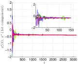
Figure 2: First component of $x_{i}^{\star}(t)$, $i\!\in\!\{1,\ldots,n\}$, zoom on selected $i$.

Then we show the evolution of the dual variables. First, note that $\mu_{i}$ is associated to the local constraint $X_{i}$ of $x_{i}$. We obtain that only $\mu_{13}$, the multiplier relative to the only active constraint, converges to a nonzero value, whereas all the other $\mu_{i}$s, associated to the inactive constraints, converge to $0$. In Figure 4 the first component of $\mu_{13}$ is plotted.

Finally, we plot the evolution of $\lambda_{i}^{j}$, $j\in\mathcal{N}_{i}$, for node $i=5$ (with $\mathcal{N}_{i}=\{3,6,10,12,14\}$), see Figure 4 for the first component. As expected the multipliers converge to nonzero values representing the “price” needed to enforce equality constraints on the primal variables $x_{i}$ and $x_{j}$.

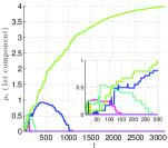
Figure 3: First component of $\mu_{i}(t)$, $i\in\{1,\ldots,n\}$.

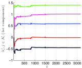
Figure 4: First component of $\lambda_{i}^{j}$, $j\in N_{i}$, with $i=5$.

6 Conclusions

In this paper we have proposed an asynchronous, distributed optimization algorithm, based on a block-coordinate dual proximal gradient method to solve separable, constrained optimization problems. The main idea is to construct a suitable, separable dual problem via a proper choice of primal constraints. Then, the dual problem is solved through a proximal gradient algorithm. Thanks to the separable structure of the dual problem in terms of local conjugate functions, the proximal gradient update results into a distributed algorithm, where each node performs a local minimization on its primal variable, and a local proximal gradient update on its dual variables. An asynchronous version of the distributed algorithm is obtained by exploiting a randomized, block-coordinate descent approach.

Appendix A Randomized coordinate descent for composite functions

Consider the following optimization problem

$$\min_{y\in{\mathbb{R}}^{N}}\;\Gamma(y):=\Phi(y)+\Psi(y)$$ (A.6)

where $\Phi:{\mathbb{R}}^{N}\to{\mathbb{R}}$ and $\Psi:{\mathbb{R}}^{N}\to{\mathbb{R}}\cup\{+\infty\}$ are convex functions.

We decompose the decision variable as $y=[y_{1}^{T}\;\ldots\;y_{n}^{T}]^{T}$ and, consistently, we decompose the space ${\mathbb{R}}^{N}$ into $n$ subspaces as follows. Let $U\in{\mathbb{R}}^{N\times N}$ be a column permutation of the $N\times N$ identity matrix and, further, let $U=[U_{1}\;U_{2}\;\ldots\;U_{n}]$ be a decomposition of $U$ into $n$ submatrices, with $U_{i}\in{\mathbb{R}}^{N\times N_{i}}$ and $\sum_{i}N_{i}=N$. Thus, any vector $y\in{\mathbb{R}}^{N}$ can be uniquely written as $y=\sum_{i}U_{i}y_{i}$ and, viceversa, $y_{i}=U_{i}^{T}y$.

We let problem (A.6) satisfy the following assumptions.

Assumption A.1 (Smoothness of $\Phi$)

The gradient of $\Phi$ is block coordinate-wise Lipschitz continuous with positive constants $L_{1},\ldots,L_{n}$. That is, for all $y\in{\mathbb{R}}^{N}$ and $s_{i}\in{\mathbb{R}}^{N_{i}}$ it holds

$$\|\nabla_{i}\Phi(y+U_{i}s_{i})-\nabla_{i}\Phi(y)\|\leq L_{i}\|s_{i}\|,$$

where $\nabla_{i}\Phi(y)$ is the $i$-th block component of $\nabla\Phi(y)$.  $\square$

Assumption A.2 (Separability of $\Psi$)

The function $\Psi$ is block-separable, i.e., it can be decomposed as $\Psi(y)=\sum_{i=1}^{n}\psi_{i}(y_{i})$, with each $\psi_{i}:{\mathbb{R}}^{N_{i}}\to{\mathbb{R}}\!\cup\!\{+\infty\}$ a proper, closed convex extended real-valued function.  $\square$

Assumption A.3 (Feasibility)

The set of minimizers of problem (A.6) is non-empty.  $\square$

Initialization: $y(0)=y_{0}$

for $t=0,1,2,\ldots$ do

   choose $i_{t}\in\{1,\ldots,n\}$ with probability $\frac{1}{n}$

   compute

$$T^{(i_{t})}\big{(}y(t)\big{)}=\mathop{\rm argmin}_{w_{i_{t}}\in{\mathbb{R}}^{N_{i_{t}}}}\Big{\{}V_{i_{t}}(y(t),w_{i_{t}})\Big{\}}$$

   where

$$V_{i_{t}}(y,s_{i_{t}}):=\nabla_{i_{t}}\Phi(y)^{T}s_{i_{t}}\!+\!\frac{L_{i_{t}}}{2}\|s_{i_{t}}\|^{2}\!+\!\psi_{i_{t}}(y_{i_{t}}\!+\!s_{i_{t}})$$

   update $y(t+1)=y(t)+U_{i_{t}}T^{(i_{t})}\big{(}y(t)\big{)}$

Algorithm 3 UCDC

The convergence result for UCDC (Algorithm 3) is given in [16, Theorem 5], here reported for completeness.

Theorem A.4 (Theorem 5, [16])

Let Assumptions A.1, A.2 and A.3 hold. Then, for any $\varepsilon\in\Big{(}0,\Gamma(y_{0})-\Gamma(y^{\star})\Big{)}$, there exists $\bar{t}(\varepsilon,\rho)>0$ such that if $y(t)$ is the random sequence generated by UCDC applied to problem (A.6), then for all $t\geq\bar{t}$ it holds that

$$\mathrm{P}\Big{(}\Gamma(y(t))-\Gamma(y^{\star})\leq\varepsilon\Big{)}\geq 1-\rho,$$

where $y^{\star}$ is a minimizer of problem (A.6), $y_{0}\in{\mathbb{R}}^{N}$ is the initial condition and $\rho\in(0,1)$ is the target confidence.  $\square$

References

- [1] K. I. Tsianos, S. Lawlor, and M. G. Rabbat, “Consensus-based distributed optimization: Practical issues and applications in large-scale machine learning,” in 50th Annual Allerton Conference on Communication, Control, and Computing (Allerton). IEEE, 2012, pp. 1543–1550.
- [2] F. Zanella, D. Varagnolo, A. Cenedese, G. Pillonetto, and L. Schenato, “Asynchronous Newton-Raphson consensus for distributed convex optimization,” in 3rd IFAC Workshop on Distributed Estimation and Control in Networked Systems, 2012.
- [3] D. Jakovetic, J. M. Freitas Xavier, and J. M. Moura, “Convergence rates of distributed Nesterov-like gradient methods on random networks,” IEEE Transactions on Signal Processing, vol. 62, no. 4, pp. 868–882, 2014.
- [4] A. Nedic and A. Olshevsky, “Distributed optimization over time-varying directed graphs,” in IEEE 52nd Annual Conference on Decision and Control (CDC). IEEE, 2013, pp. 6855–6860.
- [5] M. Akbari, B. Gharesifard, and T. Linder, “Distributed online convex optimization on time-varying directed graphs,” in Communication, Control, and Computing (Allerton), 2014 52nd Annual Allerton Conference on. IEEE, 2014.
- [6] S. S. Kia, J. Cortes, and S. Martinez, “Distributed convex optimization via continuous-time coordination algorithms with discrete-time communication,” in arXiv, 2014.
- [7] A. I. Chen and A. Ozdaglar, “A fast distributed proximal-gradient method,” in 50th Annual Allerton Conference on Communication, Control, and Computing (Allerton). IEEE, 2012, pp. 601–608.
- [8] S. Lee and A. Nedic, “Distributed random projection algorithm for convex optimization,” IEEE Journal of Selected Topics in Signal Processing, vol. 7, no. 2, pp. 221–229, 2013.
- [9] E. Wei and A. Ozdaglar, “On the O(1/k) convergence of asynchronous distributed alternating direction method of multipliers,” in Global Conference on Signal and Information Processing (GlobalSIP), 2013 IEEE. IEEE, 2013, pp. 551–554.
- [10] I. Necoara, “Random coordinate descent algorithms for multi-agent convex optimization over networks,” IEEE Transactions on Automatic Control, vol. 58, no. 8, pp. 2001–2012, 2013.
- [11] F. Facchinei, G. Scutari, and S. Sagratella, “Parallel selective algorithms for nonconvex big data optimization,” IEEE Transactions on Signal Processing, vol. 63, no. 7, pp. 1874–1889, 2015.
- [12] G. Notarstefano and F. Bullo, “Distributed abstract optimization via constraints consensus: Theory and applications,” IEEE Transactions on Automatic Control, vol. 56, no. 10, pp. 2247–2261, 2011.
- [13] M. Bürger, G. Notarstefano, and F. Allgöwer, “A polyhedral approximation framework for convex and robust distributed optimization,” IEEE Transactions on Automatic Control, vol. 59, no. 2, pp. 384–395, 2014.
- [14] A. Beck and M. Teboulle, “A fast iterative shrinkage-thresholding algorithm for linear inverse problems,” SIAM journal on imaging sciences, vol. 2, no. 1, pp. 183–202, 2009.
- [15] Y. Nesterov et al., “Gradient methods for minimizing composite objective function,” 2007.
- [16] P. Richtárik and M. Takáč, “Iteration complexity of randomized block-coordinate descent methods for minimizing a composite function,” Mathematical Programming, vol. 144, no. 1-2, pp. 1–38, 2014.
- [17] S. Boyd and L. Vandenberghe, Convex optimization. Cambridge university press, 2004.
- [18] A. Beck and M. Teboulle, “A fast dual proximal gradient algorithm for convex minimization and applications,” Operations Research Letters, vol. 42, no. 1, pp. 1–6, 2014.
- [19] N. Parikh and S. Boyd, “Proximal algorithms,” Foundations and Trends in optimization, vol. 1, no. 3, pp. 123–231, 2013.