Jacobi stability analysis of scalar field models with minimal coupling to gravity in a cosmological background

Abstract

We perform the study of the stability of the cosmological scalar field models, by using the Jacobi stability analysis, or the Kosambi-Cartan-Chern (KCC) theory. In the KCC approach we describe the time evolution of the scalar field cosmologies in geometric terms, by performing a ”second geometrization”, by considering them as paths of a semispray. By introducing a non-linear connection and a Berwald type connection associated to the Friedmann and Klein-Gordon equations, five geometrical invariants can be constructed, with the second invariant giving the Jacobi stability of the cosmological model. We obtain all the relevant geometric quantities, and we formulate the condition of the Jacobi stability for scalar field cosmologies in the second order formalism. As an application of the developed methods we consider the Jacobi stability properties of the scalar fields with exponential and Higgs type potential. We find that the Universe dominated by a scalar field exponential potential is in Jacobi unstable state, while the cosmological evolution in the presence of Higgs fields has alternating stable and unstable phases. By using the standard first order formulation of the cosmological models as dynamical systems we have investigated the stability of the phantom quintessence and tachyonic scalar fields, by lifting the first order system to the tangent bundle. It turns out that in the presence of a power law potential both these models are Jacobi unstable during the entire cosmological evolution.

I Introduction

A large number of cosmological observations, obtained initially from distant Type Ia Supernovae, have convincingly proven that the Universe has undergone a late time accelerated expansion 1n ; 2n ; 3n ; 4n . In order to explain these observations a deep change in our paradigmatic understanding of the cosmological dynamics is necessary, and many ideas have been put forward to address them. The ”standard” explanation of the late time acceleration is based on the assumption of the existence of a mysterious component, called dark energy, which is responsible for the observed characteristics of the late time evolution of the Universe.

On the other hand, the combination of the results of the observations of high redshift supernovae, and of the WMAP and of the recently released Planck data, indicate that the location of the first acoustic peak in the power spectrum of the Cosmic Microwave Background Radiation is consistent with the prediction of the inflationary model for the density parameter $\Omega$, according to which $\Omega=1$. The cosmological observations also provide strong evidence for the behavior of the parameter $w=p/\rho$ of the equation of state of the cosmological fluid, where $p$ is the pressure and $\rho$ is the density, as lying in the range $-1\leq w=p/\rho<-1/3$ acc .

In order to explain the observed cosmological dynamics, it is assumed usually that the Universe is dominated by two main components: cold (pressureless) dark matter (CDM), and dark energy (DE) with negative pressure, respectively. CDM contributes $\Omega_{m}\sim 0.3$ P2 , and its introduction is mainly motivated by the necessity of theoretically explaining the galactic rotation curves and the large scale structure formation. On the other hand, DE represents the major component of the Universe, providing $\Omega_{DE}\sim 0.7$. Dark energy is the major factor determining the recent acceleration of the Universe, as observed from the study of the distant type Ia supernovae acc . Explaining the nature and properties of dark energy has become one of the most active fields of research in cosmology and theoretical physics, with a huge number of proposed DE models( for reviews see, for instance, PeRa03 ; Pa03 ; Od ; LiM ; Mort ).

One interesting possibility for explaining DE are cosmological models containing a mixture of cold dark matter and quintessence, representing a slowly-varying, spatially inhomogeneous component 8n . From a theoretical as well as a particle physics point of view the idea of quintessence can be implemented by assuming that it is the energy associated with a scalar field $Q$, having a self-interaction potential $V(Q)$. When the potential energy density $V(Q)$ of the quintessence field is greater than the kinetic one, then it follows that the pressure $p=\dot{Q}^{2}/2-V(Q)$ associated to the quintessence $Q$-field is negative. The properties of the quintessential cosmological models have been actively considered in the physical literature (for a recent review see Tsu ). As opposed to the cosmological constant of standard general relativity, the equation of state of the quintessence field changes dynamically with time 11n . Alternative models, in which the late-time acceleration can be driven by the kinetic energy of the scalar field, called $k-$essence models, have also been proposed kessence .

Scalar fields $\phi$ that are minimally coupled to gravity via a negative kinetic energy, can also explain the recent acceleration of the Universe. Interestingly enough, they allow values of the parameter of the equation of state with $w<-1$. These types of scalar fields, known as phantom fields, have been proposed in phan1 . For phantom scalar fields the energy density and pressure are given by $\rho_{\phi}=-\dot{\phi}^{2}/2+V\left(\phi\right)$ and $p_{\phi}=-\dot{\phi}^{2}/2-V\left(\phi\right)$, respectively. The interesting properties of phantom cosmological models for dark energy have been investigated in detail in phan2 ; phan3 ; phan4 . Recent cosmological observations show that at some moment during the cosmological evolution the value of the parameter $w$ may have crossed the standard value $w=-1$, corresponding to the general relativistic cosmological constant $\Lambda$. This cosmological situation is called the phantom divide line crossing phan4 . In the case of scalar field models with cusped potentials, the crossing of the phantom divide line was investigated in phan3 . Another alternative way of explaining the phantom divide line crossing is to model dark energy by a scalar field, which is non-minimally coupled to gravity phan3 .

Scalar fields are also assumed to play a fundamental role in the evolution of the very early Universe, playing a major role in the inflationary scenario 1nn ; 2nn . Originally, the idea of inflation was proposed to provide solutions to the singularity, flat space, horizon, and homogeneity problems, to the absence of magnetic monopoles, as well as to the problem of large numbers of particles Li90 ; Li98 . However, presently it is believed that the most important feature of inflation is the generation of both initial density perturbations and of the background cosmological gravitational waves. These important cosmological parameters can be determined in many different ways, like, for example, through the study of the anisotropies of the microwave background radiation, the analysis of the local (peculiar) velocity galactic flows, of the clustering of galaxies, and the determination of the abundance of gravitationally bound structures of different types, respectively Li98 .

In many inflationary models the dynamical evolution of the early Universe is driven by a single scalar field, called the inflaton, with the inflaton rolling in some underlying self-interaction potential 1nn ; 2nn ; Li90 ; Li98 . One common approximation in the study of the inflationary evolution is the slow-roll approximation, which can be successfully used in two separate contexts. The first situation is in the study of the classical inflationary dynamics of expansion in the lowest order approximation. Hence this implies that the contribution of the kinetic energy of the inflaton field to the expansion rate is ignored. The second situation is represented by the calculation of the perturbation spectra. The standard expressions deduced for these spectra are valid in the lowest order in the slow roll approximation Co94 . Finding exact inflationary solutions of the gravitational field equations for different types of scalar field potentials is also of great importance for the understanding of the dynamics of the early Universe. Such exact solutions have been found for a large number of inflationary potentials. Moreover, the potentials allowing a graceful exit from inflation have been classified Mi .

Hence, the theoretical investigation of the scalar field models is an essential task in cosmology. Among the various methods used to study the properties of scalar fields the methods based on the applications of the mathematical formalism of the qualitative study of dynamical systems is of considerable importance.

The usefulness of dynamical systems formulation of physical models is mainly determined by their powerful predictive power. This predictive power is essentially determined by the stability of their solutions. In a realistic physical system, due to the limited precision of the measurements, some uncertainties in the initial conditions always exist. Therefore a physically meaningful mathematical model must also offer detailed and useful information on the evolution of the deviations of the possible trajectories of the dynamical system from a given reference trajectory. Hence an important requirement in mathematical modelling is the understanding of the local stability of the physical and cosmological processes. This information on the system behavior is as important as the understanding of the late-time deviations. The global stability of the solutions of the dynamical systems described by systems of non-linear ordinary differential equations is analyzed in the framework of the well-known mathematical theory of Lyapounov stability. In this mathematical approach the fundamental quantities that measure exponential deviations from a given trajectory are the so-called Lyapunov exponents 1 ; 2 . It is usually very difficult to determine the Lyapounov exponents analytically for a given dynamical system, and thus one must resort to numerical methods. On the other hand, the important problem of the local stability of the solutions of dynamical systems, described by ordinary differential equations, is less understood.

Cosmological models have been intensively investigated by using methods from dynamical systems and Lyapounov stability theory W ; C ; Liap ; cosm3 ; cosm4 . In particular, phase space analysis proved to be a very useful method for the understanding of the cosmological evolution. When studying the evolution of cosmological models, the dynamical equations can be represented by an autonomous dynamical system, described by a set of coupled - usually strongly non-linear - differential equations for the physical parameters. This representation allows the study of the Lyapunov stability of the model, without explicitly solving the field equations for the basic variables. Furthermore, the importance of the Lyapunov analysis is related to the fact that stationary points of the dynamical system correspond to exact or approximate analytic solutions of the field equations. Thus the dynamical system formulation provide a useful tool for obtaining exact or approximate solutions of the field equations in cosmologically interesting situations.

Even that the mathematical methods of the Lyapounov stability analysis are well established, the study of the stability of the dynamical systems from different points of view is extremely important. The comparison of the results of the alternative approach with the corresponding Lyapunov exponents analysis can provide a deeper understanding of the stability properties of the system. An alternative, and very powerful method for the study of the systems of the ordinary differential equations is represented by the so-called Kosambi-Cartan-Chern (KCC) theory, which was initiated in the pioneering works of Kosambi Ko33 , Cartan Ca33 and Chern Ch39 , respectively. The KCC theory was inspired and influenced by the geometry of the Finsler spaces (for a recent review of the KCC theory see rev ). From a mathematical point of view the KCC theory is a differential geometric theory of the variational equations for the deviations of the whole trajectory with respect to the nearby ones An00 . In the KCC geometrical description of the systems of ordinary differential equations one associates a non-linear connection, and a Berwald type connection to the system of equations. With the use of these geometric quantities five geometrical invariants are obtained. The most important invariant is the second invariant, also called the curvature deviation tensor, which gives the Jacobi stability of the system rev ; An00 ; Sa05 ; Sa05a . The KCC theory has been applied for the study of different physical, biochemical or technical systems (see Sa05 ; Sa05a ; An93 ; KCC ; KCC1 .

An alternative geometrization method for dynamical systems, with applications in classical mechanics and general relativity, was proposed in Pet10 and Kau , and further investigated in Pet0 ; Pet1 . The Henon-Heiles system and Bianchi type IX cosmological models were also investigated within this framework. In particular, in Pet0 a theoretical approach based on the geometrical description of dynamical systems and of their chaotic properties was developed. For the base manifold a Finsler space was introduced, whose properties allow the description of a wide class of physical systems, including those with potentials depending on time and velocities, for which the Riemannian approach is unsuitable.

It is the purpose of the present paper to consider a systematic investigation of the Jacobi stability properties of the flat homogeneous and isotropic general relativistic cosmological models. By starting from the standard Friedmann equations we perform, as a first step in our analysis, a ”second geometrization” of these equations, by associating to them a non-linear connection, and a Berwald connection, respectively. This procedure allows to obtain the so-called KCC invariants of the Friedmann equations. The second invariant, called the curvature deviation tensor, gives the Jacobi stability properties of the cosmological model. The KCC theory can be naturally applied to systems of second order ordinary differential equations. The Friedmann equations can be formulated as second order differential equations, similarly to the Klein-Gordon equation describing the scalar field. Therefore the KCC theory can be applied to matter and scalar field dominated cosmological models. We obtain the general condition for the Jacobi stability of scalar fields, which is described by two inequalities involving the second and the first derivative of the scalar field potential, the energy density of the field, as well as the time derivative of the field itself. The geodesic deviation equations describing the time variation of the deviation vector are also obtained. As an application of the developed formalism we investigate the stability properties of the scalar field cosmological models with exponential and Higgs type potentials, respectively. It turns out that the exponential potential scalar field is Jacobi unstable during its entire evolution, while the time evolution of the scalar field cosmological models with Higgs potential show a complicated dynamics with alternating stable and unstable Jacobi phases. The Jacobi stability properties of the Higgs type models are determined by the numerical value of the ratio of the self-coupling constant and the square of the mass of the Higgs particle.

The Lyapunov stability properties of the scalar field cosmological models are usually investigated by reformulating the evolution equation as a set of three first order ordinary differential equations. In order to apply the KCC theory to such systems they must be lifted to the tangent bundle. From mathematical point of view this requires to take the time derivative of the first order equations, so that their ”second geometrization” can be easily performed. We consider in detail the Jacobi stability properties of the phantom quintessence and tachyon scalar field cosmological models. We study in detail the Jacobi stability condition of these models, and we find that they are Jacobi unstable during the entire expansionary cosmological evolution.

The present paper is organized as follows. We review the basic ideas and the mathematical formalism of the KCC theory in Section II. The Jacobi stability analysis of the homogenous isotropic flat cosmological models by using the second order formulation of the dynamics is performed in Section III. We consider both the cases of the matter dominated and scalar field dominated cosmological models. As an application of the developed formalism we investigate in detail the Jacobi stability of the scalar fields with exponential potential, and Higgs potential, respectively. The Jacobi stability of the first order dynamical system formulation of scalar field cosmological models is considered in Section refsect4, in which the KCC geometrization of the phantom quintessence and tachyonic scalar field models is analyzed in detail. We discuss and conclude our results in Section V. The KCC geometric quantities giving the geometric description of the phantom quintessence and tachyon scalar field cosmologies are presented in Appendix A and Appendix B, respectively.

II Kosambi-Cartan-Chern (KCC) theory and Jacobi stability

In the present Section we briefly summarize the basic concepts and results of the KCC theory (for a detailed presentation see rev and An00 ).

II.1 Dynamical systems as paths of a semispray

In the following we denote by $\mathcal{M}$ a real, smooth $n$-dimensional manifold, and by $T\mathcal{M}$ its tangent bundle. On an open connected subset $\Omega$ of the Euclidian $(2n+1)$ dimensional space $R^{n}\times R^{n}\times R^{1}$ we introduce a $2n+1$ dimensional coordinates system $\left(x^{i},y^{i},t\right)$, $i=1,2,...,n$, where $\left(x^{i}\right)=\left(x^{1},x^{2},...,x^{n}\right)$, $\left(y^{i}\right)=\left(y^{1},y^{2},...,y^{n}\right)$ and $t$ is the time $t$. The coordinates $y^{i}$ are defined as

$$y^{i}=\left(\frac{dx^{1}}{dt},\frac{dx^{2}}{dt},...,\frac{dx^{n}}{dt}\right).$$ (1)

We assume that the time $t$ is an absolute invariant, and therefore the only admissible change of coordinates will be

$$\tilde{t}=t,\tilde{x}^{i}=\tilde{x}^{i}\left(x^{1},x^{2},...,x^{n}\right),i\in\left\{1,2,...,n\right\}.$$ (2)

Definition Punzi . A deterministic dynamical systems is a formal set of rules that describe the evolution of points in some set $S$ with respect to an external, discrete, or continuous time parameter $t$ running in another set $T$.

In a rigorous mathematical formulation, a dynamical system is a map Punzi

$$\phi:T\times S\rightarrow S,(t,x)\mapsto\phi(t,x),$$ (3)

which satisfies the condition $\phi(t,\cdot)\circ\phi(s,\cdot)=\phi(t+s,\cdot)$ for all times $t,s\in T$. In order to model realistic dynamical systems or physical processes additional structures must be added to the above definition.

In many cases the equations of motion of a dynamical system can be derived from a Lagrangian $L$ via the Euler-Lagrange equations,

$$\frac{d}{dt}\frac{\partial L}{\partial y^{i}}-\frac{\partial L}{\partial x^{i}}=F_{i},i=1,2,...,n,$$ (4)

where $F_{i}$, $i=1,2,...,n$, is the external force. For a regular Lagrangian $L$, the Euler-Lagrange equations given by Eq. (4) are equivalent to a system of second-order differential equations MHSS

$$\frac{d^{2}x^{i}}{dt^{2}}+2G^{i}\left(x^{j},y^{j}\right)=0,i\in\left\{1,2,...,n\right\},$$ (5)

where each function $G^{i}\left(x^{j},y^{j},t\right)$ is $C^{\infty}$ in a neighborhood of some initial conditions $\left(\left(x\right)_{0},\left(y\right)_{0},t_{0}\right)$ in $\Omega$.

A vector field $S$ on $T\mathcal{M}$ of the form

$$S=y^{i}\frac{\partial}{\partial x^{i}}-2G^{i}\left(x^{i},y^{i}\right)\frac{\partial}{\partial y^{i}},$$ (6)

is called a semispray S0 ; S1 ; S2 . The functions $G^{i}(x^{i},y^{i})$ are the local coefficients of the semispray, and they are defined on domains of local charts. In the particular case in which the coefficients $G^{i}=G^{i}\left(x^{i},y^{i}\right)$ are homogeneous of degree two in $y^{i}$, the vector field $S$ is called a spray.

Definition. A path of the semispray $S$ is defined as a curve $c:t\rightarrow x^{i}(t)$ on $\mathcal{M}$, with the property that its lift $c^{\prime}:t\rightarrow\left(x^{i}(t),\dot{x}^{i}(t)\right)$ to $T\mathcal{M}$ is an integral curve of $S$, that is, a curve satisfying the equation

$$\frac{d^{2}x^{i}}{dt^{2}}+2G\left(x^{i},y^{i}\right)=0.$$ (7)

Conversely, for any system of ordinary differential equations of the form (7), which is globally defined, the functions $G^{i}$ define a semispray on $T\mathcal{M}$ S1 ; S2 .

More generally, one can start from an arbitrary system of second-order differential equations of the form (5), where no a priori given Lagrangian function is assumed, and study the behavior of its trajectories by analogy with the trajectories of the Euler-Lagrange equations.

II.2 The KCC geometrization of dynamical systems

To associate a geometrical structure to the dynamical system defined by Eqs. (5), we introduce first a nonlinear connection $N$ on $M$, with coefficients $N_{j}^{i}$, defined as MHSS

$$N_{j}^{i}=\frac{\partial G^{i}}{\partial y^{j}}.$$ (8)

The nonlinear connection can be understood in terms of a dynamical covariant derivative $\nabla^{N}$ Punzi : for two vector fields $v$, $w$ defined over M, we introduce the covariant derivative $\nabla^{N}$ as

$$\nabla_{v}^{N}w=\left[v^{j}\frac{\partial}{\partial x^{j}}w^{i}+N^{i}_{j}(x,y)w^{j}\right]\frac{\partial}{\partial x^{i}}.$$ (9)

For $N_{j}^{i}(x,y)=\Gamma_{jl}^{i}(x)y^{l}$, Eq. (9) reduces to the definition of the covariant derivative for the special case of a linear connection.

For a non-singular coordinate transformations given by Eq. (2), the KCC-covariant differential of an arbitrary vector field $\theta^{i}(x)$ on the open subset $\Omega\subseteq R^{n}\times R^{n}\times R^{1}$ is defined as Sa05 ; rev

$$\frac{D\theta^{i}}{dt}=\frac{d\theta^{i}}{dt}+N_{j}^{i}\theta^{j}.$$ (10)

For $\theta^{i}=y^{i}$ we obtain

$$\frac{Dy^{i}}{dt}=N_{j}^{i}y^{j}-2G^{i}=-\epsilon^{i},$$ (11)

where the contravariant vector field $\epsilon^{i}$ on $\Omega$ is called the first KCC invariant.

II.2.1 The curvature deviation tensor

Let us now vary the trajectories $x^{i}(t)$ of the system (5) into nearby ones according to

$$\tilde{x}^{i}\left(t\right)=x^{i}(t)+\eta\xi^{i}(t),$$ (12)

where $\left|\eta\right|$ is a small parameter and $\xi^{i}(t)$ are the components of some contravariant vector field defined along the path $x^{i}(t)$. Substituting Eqs. (12) into Eqs. (5) and taking the limit $\eta\rightarrow 0$ we obtain the variational equations An93 ; An00 ; Sa05 ; Sa05a

$$\frac{d^{2}\xi^{i}}{dt^{2}}+2N_{j}^{i}\frac{d\xi^{j}}{dt}+2\frac{\partial G^{i}}{\partial x^{j}}\xi^{j}=0.$$ (13)

By using the KCC-covariant differential we can write Eq. (13) in the covariant form

$$\frac{D^{2}\xi^{i}}{dt^{2}}=P_{j}^{i}\xi^{j},$$ (14)

where we have denoted

$$P_{j}^{i}=-2\frac{\partial G^{i}}{\partial x^{j}}-2G^{l}G_{jl}^{i}+y^{l}\frac{\partial N_{j}^{i}}{\partial x^{l}}+N_{l}^{i}N_{j}^{l},$$ (15)

and we have introduced the Berwald connection $G_{jl}^{i}$, defined as rev ; An00 ; An93 ; MHSS ; Sa05 ; Sa05a

$$G_{jl}^{i}\equiv\frac{\partial N_{j}^{i}}{\partial y^{l}}.$$ (16)

The tensor $P_{j}^{i}$ is called the second KCC-invariant, or the deviation curvature tensor, and Eq. (14) is called the Jacobi equation, respectively. In both Riemann or Finsler geometry, when the system (5) describes the geodesic equations in the given geometry, Eq. (14) represents the Jacobi field equation.

The trace $P$ of the curvature deviation tensor is obtained as

$$P=P_{i}^{i}=-2\frac{\partial G^{i}}{\partial x^{i}}-2G^{l}G_{il}^{i}+y^{l}\frac{\partial N_{i}^{i}}{\partial x^{l}}+N_{l}^{i}N_{i}^{l}+\frac{\partial N_{i}^{i}}{\partial t}.$$ (17)

The third, fourth and fifth invariants of the system (5) are defined as An00

$$P_{jk}^{i}\equiv\frac{1}{3}\left(\frac{\partial P_{j}^{i}}{\partial y^{k}}-\frac{\partial P_{k}^{i}}{\partial y^{j}}\right),P_{jkl}^{i}\equiv\frac{\partial P_{jk}^{i}}{\partial y^{l}},D_{jkl}^{i}\equiv\frac{\partial G_{jk}^{i}}{\partial y^{l}}.$$ (18)

The third invariant $P_{jk}^{i}$ can be interpreted as a torsion tensor. The fourth and fifth invariants $P_{jkl}^{i}$ and $D_{jkl}^{i}$ are called the Riemann-Christoffel curvature tensor, and the Douglas tensor, respectively rev ; An00 . In Berwald spaces these tensors always exist. Generally, they can be used to describe the geometrical properties of systems of second-order differential equations.

II.3 The definition of Jacobi stability

In many physical applications the behavior of the trajectories of the dynamical system (5) in a vicinity of a point $x^{i}\left(t_{0}\right)$ is of major interest. In the following for simplicity we take $t_{0}=0$. The trajectories $x^{i}=x^{i}(t)$ can be considered as curves in the Euclidean space $\left(R^{n},\left\langle.,.\right\rangle\right)$, where $\left\langle.,.\right\rangle$ defines the canonical inner product of $R^{n}$. As for the deviation vector $\xi$ we assume that it satisfies the natural initial conditions $\xi\left(0\right)=O$ and $\dot{\xi}\left(0\right)=W\neq O$, where $O\in R^{n}$ is the null vector rev ; An00 ; Sa05 ; Sa05a .

We describe the focusing tendency of the trajectories around $t_{0}=0$ as follows: if $\left|\left|\xi\left(t\right)\right|\right|<t^{2}$, $t\approx 0^{+}$, the trajectories are bunching together. On the other hand, if $\left|\left|\xi\left(t\right)\right|\right|>t^{2}$, $t\approx 0^{+}$, the trajectories are dispersing rev ; An00 ; Sa05 ; Sa05a . Alternatively, the focusing tendency of the trajectories can be described in terms of the deviation curvature tensor: the trajectories of the system of second order differential equations (5) are bunching together for $t\approx 0^{+}$ if and only if the real parts of the eigenvalues of the deviation curvature tensor $P_{j}^{i}\left(0\right)$ are strictly negative. On the other hand the trajectories are dispersing if and only if the real parts of the eigenvalues of the tensor $P_{j}^{i}\left(0\right)$ are strictly positive rev ; An00 ; Sa05 ; Sa05a .

Based on the above intuitive considerations we can define the Jacobi stability for a second order system of differential equations as follows rev ; An00 ; Sa05 ; Sa05a :

Definition: If the system of second order differential equations (5) satisfies the initial conditions

$$\left|\left|x^{i}\left(t_{0}\right)-\tilde{x}^{i}\left(t_{0}\right)\right|\right|=0,\left|\left|\dot{x}^{i}\left(t_{0}\right)-\tilde{x}^{i}\left(t_{0}\right)\right|\right|\neq 0,$$

with respect to the norm $\left|\left|.\right|\right|$ induced by a positive definite inner product, then we call the trajectories of (5) as Jacobi stable if and only if the real parts of the eigenvalues of the deviation tensor $P_{j}^{i}$ are strictly negative everywhere. Otherwise, the trajectories are called Jacobi unstable.

The focussing/dispersing behavior of the trajectories of a system of second order ordinary differential equations near the origin is represented in Fig. 1.

Figure 1: Behavior of the trajectories near zero.

II.4 The deviation curvature tensor for two and three dimensional dynamical systems

In the important two dimensional case the curvature deviation tensor can be written in a matrix form as

$$P_{j}^{i}=\left(\begin{array}[]{c}P_{1}^{1}\;\;\;\;P_{2}^{1}\\ P_{1}^{2}\;\;\;P_{2}^{2}\end{array}\right),$$ (19)

with the eigenvalues given by

$$\lambda_{\pm}=\frac{1}{2}\left[P_{1}^{1}+P_{2}^{2}\pm\sqrt{\left(P_{1}^{1}-P_{2}^{2}\right)^{2}+4P_{2}^{1}P_{1}^{2}}\right].$$ (20)

The eigenvalues of the curvature deviation tensor can be obtained as solutions of the quadratic equation

$$\lambda^{2}-\left(P_{1}^{1}+P_{2}^{2}\right)\lambda+\left(P_{1}^{1}P_{2}^{2}-P_{2}^{1}P_{1}^{2}\right)=0.$$ (21)

A very powerful algebraic method to obtain the signs of the eigenvalues of the curvature deviation tensor is represented by the Routh-Hurwitz criteria RH . According to these criteria all of the roots of the polynomial $P(\lambda)$ are negatives or have negative real parts if the determinants of all Hurwitz matrices $\mathrm{det}\;H_{j}$, $j=1,2,..,n$, are strictly positive. For $n=2$, corresponding to the case of Eq. (21), the Routh-Hurwitz criteria takes the simple form

$$P_{1}^{1}+P_{2}^{2}<0,\;\;P_{1}^{1}P_{2}^{2}-P_{2}^{1}P_{1}^{2}>0.$$ (22)

The curvature properties along a given geodesic are described by the eigenvalues of the deviation curvature tensor $\lambda_{\pm}$, which are invariant functions on the tangent space. Moreover, once they are known, we can introduce two quantities that can characterize the way the geodesic explores the base manifold. They are defined as the (half) of the Ricci curvature scalar along the flow, $\kappa$, and the anisotropy $\theta$, given by

$$\kappa=\frac{1}{2}\left(\lambda_{+}+\lambda_{-}\right)=\frac{P}{2}=\frac{P_{1}^{1}+P_{2}^{2}}{2},$$ (23)

and

$$\theta=\frac{1}{2}\left(\lambda_{+}-\lambda_{-}\right)=\frac{\sqrt{\left(P_{1}^{1}-P_{2}^{2}\right)^{2}+4P_{2}^{1}P_{1}^{2}}}{2},$$ (24)

respectively.

In the case of a three-dimensional dynamical system with $n=3$, the characteristic equation of the matrix of the curvature deviation tensor becomes

$$\lambda^{3}-\left(P^{1}_{1}+P^{2}_{2}+P^{3}_{3}\right)\lambda^{2}-\Bigg{[}-P^{1}_{1}\left(P^{2}_{2}+P^{3}_{3}\right)+$$

$$P^{1}_{2}P^{2}_{1}+P^{1}_{3}P^{3}_{1}-P^{2}_{2}P^{3}_{3}+P^{2}_{3}P^{3}_{2}\Bigg{]}\lambda-$$

$$\Bigg{[}P^{1}_{1}\left(P^{2}_{2}P^{3}_{3}-P^{2}_{3}P^{3}_{2}\right)-P^{1}_{2}\left(P^{2}_{1}P^{3}_{3}-P^{2}_{3}P^{3}_{1}\right)+$$

$$P^{1}_{3}\left(P^{2}_{1}P^{3}_{2}-P^{2}_{2}P^{3}_{1}\right)\Bigg{]}=0.$$ (25)

Therefore the conditions of the Jacobi stability for a three-dimensional system of second order ordinary differential equations can be formulated as follows:

$$\Sigma=P^{1}_{1}+P^{2}_{2}+P^{3}_{3}<0,$$ (26)

$$\Phi=-P^{1}_{1}\left(P^{2}_{2}+P^{3}_{3}\right)+P^{1}_{2}P^{2}_{1}+P^{1}_{3}P^{3}_{1}-P^{2}_{2}P^{3}_{3}+P^{2}_{3}P^{3}_{2}<0,$$ (27)

$$\Psi=P^{1}_{1}\left(P^{2}_{2}P^{3}_{3}-P^{2}_{3}P^{3}_{2}\right)-P^{1}_{2}\left(P^{2}_{1}P^{3}_{3}-P^{2}_{3}P^{3}_{1}\right)+$$

$$P^{1}_{3}\left(P^{2}_{1}P^{3}_{2}-P^{2}_{2}P^{3}_{1}\right)<0,$$ (28)

$$\Omega=\left(P^{1}_{1}+P^{2}_{2}+P^{3}_{3}\right)\Bigg{[}-P^{1}_{1}\left(P^{2}_{2}+P^{3}_{3}\right)+P^{1}_{2}P^{2}_{1}+$$

$$P^{1}_{3}P^{3}_{1}-P^{2}_{2}P^{3}_{3}+P^{2}_{3}P^{3}_{2}\Bigg{]}-\Bigg{[}P^{1}_{1}\left(P^{2}_{2}P^{3}_{3}-P^{2}_{3}P^{3}_{2}\right)-$$

$$P^{1}_{2}\Big{(}P^{2}_{1}P^{3}_{3}-P^{2}_{3}P^{3}_{1}\Big{)}+P^{1}_{3}\left(P^{2}_{1}P^{3}_{2}-P^{2}_{2}P^{3}_{1}\right)\Bigg{]}>0.$$

III Jacobi stability analysis of isotropic matter dominated and scalar field cosmologies

In the present Section we use the KCC approach for the study of the dynamical properties of the matter dominated and scalar field cosmologies. We explicitly obtain the non-linear and Berwald connections, and the deviation curvature tensors. The eigenvalues of the deviation curvature tensor are also obtained, and we study their properties in the equilibrium points of the matter dominated model. The study of the sign of the eigenvalues allows us to obtain the Jacobi stability properties of the fixed points of the matter field dominated cosmological models. Next, we proceed to a detailed analysis of the scalar field cosmologies in the framework of the KCC theory. A full ”second geometric” description is introduced, and the time evolution of the relevant physical and geometrical parameters is obtained. In particular, the nature of the Jacobi stability is analyzed in detail. In the present study we restrict our analysis to the case of the flat Friedmann-Robertson-Walker metric, given by

$$ds^{2}=dt^{2}-a^{2}(t)\left(dx^{2}+dy^{2}+dz^{2}\right),$$ (30)

where $a$ is the scale factor.

III.1 Jacobi stability of matter dominated cosmological models

For a Universe filled with pressureless dust and radiation only, the cosmological expansion is described mathematically by the Friedmann equations, which take the well-known form

$$3H^{2}=\rho_{m}+\rho_{r}+\Lambda,\dot{H}=-\frac{1}{2}\left(\rho_{m}+\frac{4}{3}\rho_{r}\right),$$ (31)

$$\dot{\rho}_{m}+3H\rho_{m}=0,\dot{\rho}_{r}+4H\rho_{r}=0$$ (32)

where a dot denotes the derivative with respect to the time $t$. In Eqs. (31) and (32) $H=\dot{a}/a$ denotes the Hubble function, $\rho_{m}$ is the baryonic matter energy density, $\rho_{r}$ is the energy density of the radiation, while $\Lambda$ is the cosmological constant.

III.1.1 Friedmann equations as an autonomous dynamical system

In order to reformulate the cosmological evolutions equations as a dynamical system, we need to introduce first the density parameters $\left(\Omega_{m},\Omega_{r},\Omega_{\Lambda}\right)$ of the matter, radiation and cosmological constant, defined as

$$\Omega_{m}=\frac{\rho_{m}}{3H^{2}},\Omega_{r}=\frac{\rho_{r}}{3H^{2}},\Omega_{\Lambda}=\frac{\Lambda}{3H^{2}}.$$ (33)

The density parameters satisfy the normalization relation

$$\Omega_{m}+\Omega_{r}+\Omega_{\Lambda}=1.$$ (34)

As the basic variables $(x,y)$ in the phase space we adopt the quantities $x\equiv\Omega_{r}$, and $y\equiv\Omega_{\Lambda}$, respectively cosm3 . Then the density parameter of the mater is given by $\Omega_{m}=1-x-y$, and the range of the variables $\left(x,y,\Omega_{m}\right)$ is $0\leq x\leq 1$, $0\leq y\leq 1$, and $0\leq\Omega_{m}\leq 1$. To describe the cosmological dynamics we define the physically significant phase space as $\Phi=\left\{(x,y):x+y\leq 1,0\leq x\leq 1,0\leq y\leq 1\right\}$. Next we take the time derivatives of $x$ and $y$ with respect to the time $t$, and, after introducing the new time variable $\tau=\ln a(t)$, we can formulate the Friedmann equations as an autonomous dynamical system given by cosm3

$$\frac{dx}{d\tau}=-x(1-x+3y),$$ (35)

$$\frac{dy}{d\tau}=(3+x-3y)y.$$ (36)

The critical points of the system (35) and (36) in the phase space region defined by $\Psi$ are obtained by solving the algebraic equations $x(1-x+3y)=0$ and $(3+x-3y)y=0$, respectively, and are given by

$$P_{dS}=\{x=0,y=1\},P_{r}=\{x=1,y=0\},$$

$$P_{m}=\{x=0,y=0\}.$$ (37)

The Lyapunov stability properties of the system follows from the study of the Jacobian matrix

$$J=\begin{pmatrix}-1+2x-3y&-3x\\ y&3+x-6y\end{pmatrix}.$$ (38)

The critical point of the system (35) and (36) have a clear cosmological interpretation. Thus, the critical point $P_{dS}=(0,1)$, with $\Omega_{\Lambda}=1$, has $a(t)\propto\exp\left(\sqrt{\Lambda/3}t\right)$, and is associated to an accelerated de Sitter type expansion, being a future attractor cosm4 . The critical point $P_{r}=(1,0)$, with $\Omega_{r}=1$ and $a(t)\propto\sqrt{t}$, corresponds to the radiation-dominated era in the cosmological evolution of the Universe, and is a source point, or a past attractor. Finally, the critical point $P_{m}(0,0)$, with $\Omega_{m}=1$ and $a(t)\propto t^{2/3}$, corresponds to the decelerating matter-dominated phase of the cosmological expansion. It turns out that $P_{m}$ is a saddle critical point cosm4 .

III.1.2 The KCC geometrization and the Jacobi stability of the Friedmann equations

In order to apply the KCC theory to the cosmological dynamical system given by equations (35) and (36), we first relabel the variables as $x\equiv x^{1}$ and $y\equiv x^{2}$. We also denote $y^{1}=dx^{1}/d\tau$ and $y^{2}=dx^{2}/d\tau$, respectively. Hence we obtain

$$\frac{dx^{1}}{d\tau}=-x^{1}\left(1-x^{1}+3x^{2}\right)=f\left(x^{1},x^{2}\right),$$ (39)

$$\frac{dx^{2}}{d\tau}=\left(3+x^{1}-3x^{2}\right)x^{2}=g\left(x^{1},x^{2}\right).$$ (40)

Next, we take the derivative with respect to $\tau$ of Eqs. (39) and (40), respectively, thus obtaining the following lift on the tangent bundle of the cosmological dynamical system,

$$\frac{d^{2}x^{1}}{d\tau^{2}}=\left(-1+2x^{1}-3x^{2}\right)y^{1}-3x^{1}y^{2},$$ (41)

$$\frac{d^{2}x^{2}}{d\tau^{2}}=x^{2}y^{1}+\left(3+x^{1}-6x^{2}\right)y^{2}.$$ (42)

By comparison with Eqs. (5) we obtain immediately

$$G^{i}\left(x^{1},x^{2},y^{1},y^{2}\right)=$$

$$-\frac{1}{2}\begin{pmatrix}\left(-1+2x^{1}-3x^{2}\right)y^{1}\;\;\;\;\;\;\;\;\;-3x^{1}y^{2}\\ \;\;\;\;x^{2}y^{1}\;\;\;\;\;\;\;\;\;\;\;\;\;\;\;\;\;\;\;\;\left(3+x^{1}-6x^{2}\right)y^{2}\end{pmatrix}.$$ (43)

Hence the components of the non-linear connection $\left(N\right)=N_{i}^{j}$ associated to the matter dominated cosmological dynamical system in the presence of a cosmological constant are obtained as

$$\left(N\right)=N_{i}^{j}=-\frac{1}{2}\begin{pmatrix}-1+2x^{1}-3x^{2}&-3x^{1}\\ x^{2}&3+x^{1}-6x^{2}\end{pmatrix}.$$ (44)

For the components of the deviation tensor $P=P_{i}^{j}$ we obtain

$$P=\frac{1}{2}\begin{pmatrix}H_{f}\cdot y&H_{g}\cdot y\end{pmatrix}^{t}+\frac{1}{4}J^{2}\left(f,g\right),$$ (45)

where

$$H_{f}=\begin{pmatrix}f_{11}&f_{12}\\ f_{21}&f_{22}\end{pmatrix},$$ (46)

is the Hessian of $f$, and $H_{g}$ is the Hessian of $g$. Explicitly, the curvature deviation tensor for the Friedmann cosmological dynamical system can be obtained as

$$\left.P\right|_{\left(y^{1}=0,y^{2}=0\right)}=\left(\begin{array}[]{cc}\frac{1}{4}(-2x^{1}+3x^{2}+1)^{2}+\frac{3x^{1}x^{2}}{2}&\frac{3}{2}x^{1}(x^{1}-6x^{2}+3)+\frac{3}{4}x^{1}(-2x^{1}+3x^{2}+1)\\ (x^{1}-6x^{2}+3)x^{2}+\frac{1}{2}(-2x^{1}+3x^{2}+1)x^{2}&(x^{1}-6x^{2}+3)^{2}+\frac{3x^{1}x^{2}}{2}\end{array}\right).$$ (47)

By evaluating $P$ at the critical points gives

$$\left.P\right|_{\left(y^{1}=0,y^{2}=0,x^{1}=x^{1}_{cr},x^{2}=x^{2}_{cr}\right)}=\frac{1}{4}A^{2},$$ (48)

where $A=\left.J\right|_{\left(y^{1}=0,y^{2}=0,x^{1}=x^{1}_{cr},x^{2}=x^{2}_{cr}\right)}$.

III.1.3 Jacobi stability of the critical points of the matter dominated cosmological models

In order to obtain the Jacobi stability of the critical points of the cosmological model described by Eqs. (35) and (36), we need to compute the numerical values of the curvature deviation tensor at the critical points. At the critical point $P_{dS}=\left(x^{1}=0,x^{2}=1\right)$ the curvature deviation tensor takes the form

$$\left.P\right|_{\left(y^{1}=0,y^{2}=0,x^{1}=0,x^{2}=1\right)}=\left(\begin{array}[]{cc}4&0\\ -1&9\end{array}\right)$$ (49)

and has the eigenvalues $\lambda_{1}=4$ and $\lambda_{2}=9$. Hence it follows that the critical point $P_{dS}$ of the standard $\Lambda$CDM cosmological model is Jacobi unstable. For the critical point $P_{r}=\left(x^{1}=1,x^{2}=0\right)$, we find

$$\left.P\right|_{\left(y^{1}=0,y^{2}=0,x^{1}=1,x^{2}=0\right)}=\left(\begin{array}[]{cc}\frac{1}{4}&\frac{21}{4}\\ 0&16\end{array}\right),$$ (50)

with the corresponding eigenvalues of the curvature deviation tensor obtained as $\lambda_{1}=16$ and $\lambda_{2}=1/4$. Hence, the critical point $P_{r}$ is also Jacobi unstable. Finally, for the last critical point $P_{m}=(0,0)$ we obtain

$$\left.P\right|_{\left(y^{1}=0,y^{2}=0,x^{1}=0,x^{2}=0\right)}=\left(\begin{array}[]{cc}\frac{1}{4}&0\\ 0&9\end{array}\right),$$ (51)

with the eigenvalues $\lambda_{1}=9$, $\lambda_{2}=1/4$. Hence, we obtain the result that all the critical points of the dynamical system equivalent to the cosmological Friedmann equations are Jacobi unstable.

III.2 The cosmological evolution equations in the presence of minimally coupled scalar fields

Let us consider a rather general class of scalar field models, minimally coupled to the gravitational field, for which the Lagrangian density in the Einstein frame reads

$$L=\frac{1}{2\kappa}\sqrt{\left|g\right|}\left\{R+\kappa\left[g^{\mu\nu}\left(\partial_{\mu}\phi\right)\left(\partial_{\nu}\phi\right)-2V\left(\phi\right)\right]\right\}\,,$$ (52)

where $R$ is the curvature scalar, $\phi$ is the scalar field, $V\left(\phi\right)$ is the self-interaction potential and $\kappa=8\pi G/c^{4}$ is the gravitational coupling constant, respectively. In the following, we use natural units with $c=8\pi G=\hbar=1$, and we adopt as our signature for the metric $\left(+1,-1,-1,-1\right)$, as is common in particle physics.

For a flat FRW scalar field dominated Universe the evolution of a cosmological model is determined by the system of the field equations

$$3\left(\frac{\dot{a}}{a}\right)^{2} = \rho_{\phi}=\frac{\dot{\phi}^{2}}{2}+V\left(\phi\right),$$ (53)

$$2\frac{\ddot{a}}{a}+\left(\frac{\dot{a}}{a}\right)^{2} = -p_{\phi}=-\frac{\dot{\phi}^{2}}{2}+V\left(\phi\right),$$ (54)

and the evolution equation for the scalar field

$$\ddot{\phi}+3\frac{\dot{a}}{a}\dot{\phi}+V^{\prime}\left(\phi\right)=0,$$ (55)

where the overdot denotes the derivative with respect to the time-coordinate $t$, and the prime denotes the derivative with respect to the scalar field $\phi$, respectively. By substituting $\dot{a}/a$ from Eq. (53) into Eqs. (54) and (55) we can reformulate the dynamics of the scalar field cosmological models in terms of two second order non-linear ordinary differential equations, given by

$$\ddot{a}+\frac{1}{3}\left[\dot{\phi}^{2}-V(\phi)\right]a=0,$$ (56)

and

$$\ddot{\phi}+\sqrt{3}\sqrt{\frac{\dot{\phi}^{2}}{2}+V\left(\phi\right)}\dot{\phi}+V^{\prime}\left(\phi\right)=0,$$ (57)

respectively.

III.2.1 The non-linear and Berwald connections, and the KCC invariants of the scalar field cosmological models

In the following we introduce a new notation for the dependent variables $a$ and $\phi$, and for their time derivatives, respectively, as

$$a=x^{1},\phi=x^{2},\dot{a}=y^{1},\dot{\phi}=y^{2}.$$ (58)

The cosmological dynamics of scalar field dominated Universes can be formulated as a second order differential system, given by two second order differential equations of the form

$$\frac{d^{2}x^{i}}{dt^{2}}+2G^{i}\left(x^{i},y^{i}\right)=0,i=1,2.$$ (59)

From Eqs. (56) and (57) it follows immediately that

$$G^{1}\left(a,\phi,\dot{a},\dot{\phi}\right)=\frac{1}{6}\left[\dot{\phi}^{2}-V(\phi)\right]a,$$ (60)

and

$$G^{2}\left(a,\phi,\dot{a},\dot{\phi}\right)=\frac{V^{\prime}(\phi)}{2}+\frac{\sqrt{3}}{2}\dot{\phi}\sqrt{V(\phi)+\frac{\dot{\phi}^{2}}{2}},$$ (61)

respectively. Therefore we first obtain the components of the non-linear connection as

$$N_{1}^{1}=\frac{\partial G^{1}\left(a,\phi,\dot{a},\dot{\phi}\right)}{\partial\dot{a}}=0,$$ (62)

$$N_{2}^{1}=\frac{\partial G^{1}\left(a,\phi,\dot{a},\dot{\phi}\right()}{\partial\dot{\phi}}=\frac{a\dot{\phi}}{3},$$ (63)

$$N_{1}^{2}=\frac{\partial G^{2}\left(a,\phi,\dot{a},\dot{\phi}\right)}{\partial\dot{a}}=0,$$ (64)

$$N_{2}^{2} = \frac{\partial G^{2}\left(a,\phi,\dot{a},\dot{\phi}\right)}{\partial\dot{\phi}}=\sqrt{\frac{3}{2}}\frac{\left(V(\phi)+\dot{\phi}^{2}\right)}{\sqrt{2V(\phi)+\dot{\phi}^{2}}}=$$

. $$\frac{\sqrt{3}}{2}\frac{2\rho_{\phi}-V(\phi)}{\sqrt{\rho_{\phi}}}.$$ (65)

For the non-zero components of the Berwald connection, defined as

$$G_{jl}^{i}=\frac{\partial N_{j}^{i}}{\partial y^{l}},i,j,l=1,2,$$ (66)

we obtain

$$G_{22}^{1}=\frac{\partial N_{2}^{1}}{\partial y^{2}}=\frac{1}{3}a,$$ (67)

$$G_{22}^{2}=\frac{\partial N_{2}^{2}}{\partial y^{2}}=\sqrt{\frac{3}{2}}\frac{\dot{\phi}\left(3V(\phi)+\dot{\phi}^{2}\right)}{\left(2V(\phi)+\dot{\phi}^{2}\right)^{3/2}}.$$ (68)

The components of the first KCC invariant of the minimally coupled scalar field model are obtained as

$$\epsilon^{1}=2G^{1}\left(a,\phi,\dot{a},\dot{\phi}\right)-N_{2}^{1}\dot{\phi}=-\frac{1}{3}aV\left(\phi\right),$$ (69)

and

$$\epsilon^{2} = 2G^{2}\left(a,\phi,\dot{a},\dot{\phi}\right)-N_{2}^{2}\dot{\phi}=V^{\prime}\left(\phi\right)+$$ (70)

$$\sqrt{\frac{3}{2}}\frac{\dot{\phi}V\left(\phi\right)}{\sqrt{2V\left(\phi\right)+\dot{\phi}^{2}}}=V^{\prime}\left(\phi\right)+\frac{\sqrt{3}}{2}\frac{\dot{\phi}V(\phi)}{\sqrt{\rho_{\phi}}},$$

respectively.

The components of the curvature deviation tensor for minimally coupled scalar field cosmological models are given by

$$P_{1}^{1}=\frac{1}{3}\left[V(\phi)-\dot{\phi}^{2}\right],$$ (71)

$$P_{2}^{1}=\frac{\dot{a}\dot{\phi}}{3}-\frac{1}{\sqrt{6}}\frac{a\dot{\phi}V(\phi)}{\sqrt{2V(\phi)+\dot{\phi}^{2}}},$$ (72)

$$P_{1}^{2}=0,$$ (73)

$$P_{2}^{2} = -V^{\prime\prime}(\phi)-\frac{\sqrt{6}\dot{\phi}V^{\prime}(\phi)}{\sqrt{2V(\phi)+\dot{\phi}^{2}}}+$$ (74)

$$\frac{9V(\phi)^{2}}{2\left[2V(\phi)+\dot{\phi}^{2}\right]}-\frac{3V(\phi\ )}{2}.$$

For the trace of the curvature deviation tensor we obtain

$$P = P_{1}^{1}+P_{2}^{2}=\frac{1}{6}\Bigg{\{}-2\left[3V^{\prime\prime}(\phi)+\dot{\phi}^{2}\right]-$$ (76)

$$\frac{6\sqrt{6}\dot{\phi}V^{\prime}(\phi)}{\sqrt{2V(\phi)+\dot{\phi}^{2}}}+\frac{27V^{2}(\phi)}{2V(\phi)+\dot{\phi}^{2}}-7V(\phi)\Bigg{\}},$$

while for $\chi=P_{1}^{1}P_{2}^{2}-P_{2}^{1}P_{1}^{2}=P_{1}^{1}P_{2}^{2}$ we have

$$\chi = \frac{1}{3}\left[V(\phi)-\dot{\phi}^{2}\right]\times\Bigg{[}-V^{\prime\prime}(\phi)-\frac{\sqrt{6}\dot{\phi}V^{\prime}(\phi)}{\sqrt{2V(\phi)+\dot{\phi}^{2}}}+$$ (77)

$$\frac{9V^{2}(\phi)}{2\left(2V(\phi)+\dot{\phi}^{2}\right)}-\frac{3V(\phi)}{2}\Bigg{]}.$$

Therefore if the conditions $P_{1}^{1}+P_{2}^{2}<0$ and $\;P_{1}^{1}P_{2}^{2}-P_{2}^{1}P_{1}^{2}>0$ are simultaneously satisfied, the scalar field cosmological model is Jacobi stable. These conditions allows us to formulate the following

Jacobi stability condition of isotropic and homogeneous scalar field cosmological models. If the parameters $\left(V(\phi),\rho_{\phi},p_{\phi},\dot{\phi}\right)$ of a homogeneous scalar field in an isotropic flat FRW geometry simultaneously satisfy the conditions

$$V^{\prime\prime}(\phi)>\frac{9}{4}\frac{V^{2}(\phi)}{\rho_{\phi}}-\frac{3}{2}\rho_{\phi}-\frac{1}{2}V(\phi)-\sqrt{3}\frac{\dot{\phi}V^{\prime}(\phi)}{\sqrt{\rho_{\phi}}},$$

$$\left[2p_{\phi}+V(\phi)\right]\times$$

$$\left[V^{\prime\prime}(\phi)+\frac{\sqrt{3}\dot{\phi}V^{\prime}(\phi)}{\rho_{\phi}}+\frac{3V(\phi)}{2}-\frac{9V^{2}(\phi)}{4\rho_{\phi}}\right]>0,$$

the corresponding cosmological model is Jacobi stable, and Jacobi unstable otherwise.

For the variational differential equations determining the deviation vector $\xi$, we obtain

$$3\frac{d^{2}\xi^{1}}{dt^{2}}+2a\dot{\phi}\frac{d\xi^{2}}{dt}+\left[\dot{\phi}^{2}-V(\phi)\right]\xi^{1}(t)-aV^{\prime 2}(t)=0,$$ (78)

and

$$\frac{d^{2}\xi^{2}}{dt^{2}}+\frac{\sqrt{6}\left[V(\phi)+\dot{\phi}^{2}\right]}{\sqrt{2V(\phi)+\dot{\phi}^{2}}}\frac{d\xi^{2}}{dt}+$$

$$\left[V^{\prime\prime}(\phi)+\frac{\sqrt{\frac{3}{2}}\dot{\phi}V^{\prime}(\phi\ )}{\sqrt{2V(\phi)+\dot{\phi}^{2}}}\right]\xi^{2}(t)=0,$$ (79)

respectively.

In the case of the isotropic cosmological scalar field models the third, fourth and fifth KCC invariants, as defined by Eqs. (18), are identically equal to zero.

III.2.2 Applications: the case of the scalar field with exponential self-interaction potential

As an application of the KCC geometrization of the scalar field cosmological models we will consider the case of a scalar field with an exponential self-interaction potential of the form

$$V(\phi)=V_{0}e^{\pm\lambda\phi},$$ (80)

where $V_{0}$ and $\lambda$ are constants. The cosmological equations describing the time evolution of this scalar field model are

$$\ddot{a}+\frac{1}{3}\left[\dot{\phi}^{2}-V_{0}e^{\pm\lambda\phi}\right]a=0,$$ (81)

and

$$\ddot{\phi}+\sqrt{3}\sqrt{\frac{\dot{\phi}^{2}}{2}+V_{0}e^{\pm\lambda\phi}}\dot{\phi}\pm\lambda V_{0}e^{\pm\lambda\phi}=0,$$ (82)

respectively. By introducing a new time variable $\tau=\sqrt{V_{0}}t$, it turns out that the system of Eqs. (81) and (82) can be written as

$$\frac{d^{2}a}{d\tau^{2}}+\frac{1}{3}\left[\left(\frac{d\phi}{d\tau}\right)^{2}-e^{\pm\lambda\phi}\right]a=0,$$ (83)

$$\frac{d^{2}\phi}{d\tau^{2}}+\sqrt{3}\sqrt{\frac{1}{2}\left(\frac{d\phi}{d\tau}\right)^{2}+e^{\pm\lambda\phi}}\frac{d\phi}{d\tau}\pm\lambda e^{\pm\lambda\phi}=0.$$ (84)

The system of Eqs. (83)-(84) must be integrated with the initial conditions $a(0)=a_{0}$, $\dot{a}(0)=a_{0}H_{0}$, $\phi\left(0\right)=\phi_{0}$, and $\dot{\phi}\left(0\right)=\dot{\phi}_{0}$, respectively.

The variations of the scale factor and of the scalar field of the exponential potential scalar field filled Universe are presented, for different values of the parameter $\lambda$, in Fig. 2. In order to numerically solve the field equations we have used the initial conditions $a(0)=0$, $\phi(0)=0.001$, $\dot{a}(0)=1$, and $\dot{\phi}(0)=-0.001$, respectively.

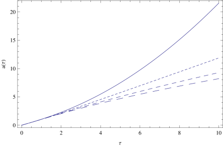
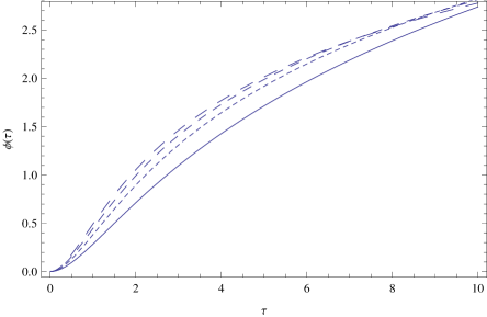
Figure 2: Variation of the scale factor of the Universe (left figure) and of the scalar field (right figure) as a function of the dimensionless time $\tau$ for the scalar field with exponential potential, for different values of the parameter $\lambda$: $\lambda=-1$ (solid curve), $\lambda=-\sqrt{2}$ (dotted curve), $\lambda=-\sqrt{3}$ (short dashed curve), and $\lambda=-2$ (dashed curve).

As one can see from the figures, the scale factor is a monotonically increasing function of time, while the scalar field also increases during the cosmological evolution. The time variation of the scalar field potential is presented in Fig. 3.

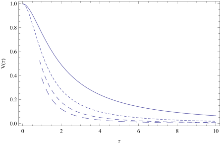
Figure 3: Variation of the scalar field potential $V=\exp(-\lambda\phi)$ as a function of the dimensionless time $\tau$ for different values of the parameter $\lambda$: $\lambda=-1$ (solid curve), $\lambda=-\sqrt{2}$ (dotted curve), $\lambda=-\sqrt{3}$ (short dashed curve), and $\lambda=-2$ (dashed curve).

The scalar field potential is a monotonically decreasing function of time, which tends, in the large time limit, to zero. The time variations of the KCC invariant $2\kappa=P_{1}^{1}+P_{2}^{2}$ and $\chi=P_{1}^{1}P_{2}^{2}-P_{2}^{1}P_{2}^{1}$ are represented in Figs. 4.

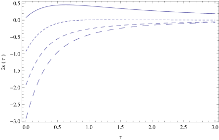
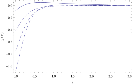
Figure 4: Time variations of the KCC invariants $2\kappa=P_{1}^{1}+P_{2}^{2}$ (left figure) and $\chi=P_{1}^{1}P_{2}^{2}-P_{2}^{1}P_{2}^{1}$ (right figure) for a Universe filled with a scalar field with exponential potential, for different values of the parameter $\lambda$: $\lambda=-1$ (solid curve), $\lambda=-\sqrt{2}$ (dotted curve), $\lambda=-\sqrt{3}$ (short dashed curve), and $\lambda=-2$ (dashed curve).

In order for the considered model of the Universe be stable, the invariants must simultaneously satisfy the conditions $2\kappa<0$ and $\chi>0$, respectively. As one can see from the Figures, from the chosen set of parameters, these conditions are not satisfied for any interval of time during the cosmological evolution. Therefore it follows that during its entire evolution an exponential potential scalar field Universe is in a Jacobi unstable state. Finally, in Figs. 5 we present the time variation of the components of the deviation vector $\xi^{i}$, $i=1,2$.

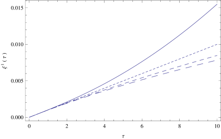
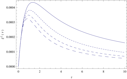
Figure 5: Time variations of the deviation vector components $\xi^{1}$ (left figure) and $\xi^{2}$ (right figure) for a Universe filled with a scalar field with exponential potential, for different values of the parameter $\lambda$: $\lambda=-1$ (solid curve), $\lambda=-\sqrt{2}$ (dotted curve), $\lambda=-\sqrt{3}$ (short dashed curve), and $\lambda=-2$ (dashed curve).

The component $\xi^{1}$ of the deviation vector increases exponentially in time, indicating that the trajectories do diverge exponentially near the origin. Thus, this result also confirms the presence of the Jacobi instability for the exponential potential scalar field cosmology.

III.2.3 Scalar fields with Higgs potential

As a next case of the investigation of the Jacobi stability of a cosmological scalar field model we consider that the Universe is filled with a Higgs-like field, with self-interaction potential given by

$$V(\phi)=V_{0}+\frac{1}{2}M^{2}\phi^{2}+\frac{\lambda}{4}\phi^{4},$$ (85)

where $V_{0}$ is a constant, and $M^{2}<0$ is related to the mass of the Higgs boson by the relation $m_{H}=V^{\prime\prime 2}$, where $v^{2}=-M^{2}/\lambda$ gives the minimum of the potential. The Higgs self-coupling constant $\lambda\approx 1/8$ Higgs , a value inferred based on the determination of $m_{H}$ from accelerator experiments. By introducing a new dimensionless time variable $\tau=Mt$, the basic equations determining the cosmological evolution are given by

$$\frac{d^{2}a}{d\tau^{2}}+\frac{1}{3}\left[\frac{1}{2}\left(\frac{d\phi}{d\tau}\right)^{2}-v_{0}+\frac{1}{2}\phi^{2}-\eta\phi^{4}\right]=0,$$ (86)

$$\frac{d^{2}\phi}{d\tau^{2}}+\sqrt{3}\sqrt{\frac{1}{2}\left(\frac{d\phi}{d\tau}\right)^{2}+v_{0}-\frac{1}{2}\phi^{2}+\eta\phi^{4}}\;\frac{d\phi}{d\tau}-\phi+4\eta\phi^{3}=0,$$ (87)

where $v_{0}=V_{0}/M^{2}$ and $\eta=\lambda/4M^{2}>0$, respectively. The time variations of the scale factor of the Higgs field filled Universe and of the scalar field are represented in Fig. 6. To numerically integrate the gravitational field equations, we have fixed the value of the constant $v_{0}$ to $v_{0}=0.005$, and we have adopted as initial conditions the values the initial conditions $a(0)=a_{0}$, $\dot{a}(0)=a_{0}H_{0}$, $\phi\left(0\right)=\phi_{0}$, and $\dot{\phi}\left(0\right)=\dot{\phi}_{0}$, respectively.

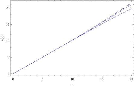
Figure 6: Variation of the scale factor of the Universe (left figure) and of the scalar field (right figure) as a function of the dimensionless time $\tau$ for the scalar field with Higgs type self-interaction potential, for different values of the parameter $\eta$: $\eta=10$ (solid curve), $\eta=20$ (dotted curve), $\eta=30$ (short dashed curve), and $\eta=40$ (dashed curve).

The Universe filled with a Higgs type scalar field is expanding, with the scale factor monotonically increasing in time. In the initial phases of the expansion the scale factor can be approximated by a linearly increasing function of time. The Higgs scalar field $\phi$ keeps a constant value in the initial stages of the evolution, followed by a rapid increase associated with an oscillatory behavior with a decreasing amplitude, associated with the energy dissipation. The variation of the Higgs potential is represented in Fig. 7.

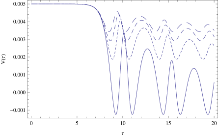
Figure 7: Variation of the Higgs type potential of the scalar field as a function of the dimensionless time $\tau$ for different values of the parameter $\eta$: $\eta=10$ (solid curve), $\eta=20$ (dotted curve), $\eta=30$ (short dashed curve), and $\eta=40$ (dashed curve).

After an initial phase in which the potential is constant, rapid oscillations with decreasing amplitude do follow, and the potential decays in time. The variation of the KCC invariants $2\kappa$ and $\chi$ is represented in Fig. 8.

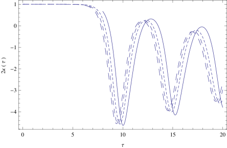
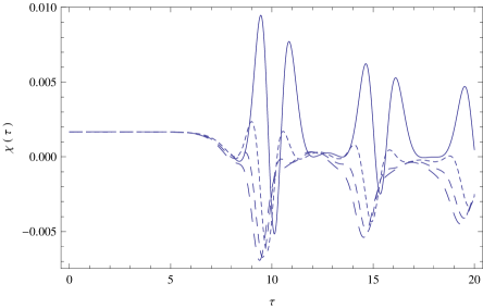
Figure 8: Time variations of the KCC invariants $2\kappa=P_{1}^{1}+P_{2}^{2}$ (left figure) and $\chi=P_{1}^{1}P_{2}^{2}-P_{2}^{1}P_{2}^{1}$ (right figure) for a Universe filled with a Higgs type scalar field, for different values of the parameter $\eta$: $\eta=10$ (solid curve), $\eta=20$ (dotted curve), $\eta=30$ (short dashed curve), and $\eta=40$ (dashed curve).

Jacobi stability of the cosmological model with Higgs type scalar field requires the conditions $2\kappa<0$ and $\chi>0$ to be simultaneously satisfied. The Jacobi stable/unstable regions formed during the cosmological expansion of scalar field cosmologies with Higgs self-interacting potential are presented in Fig. 9.

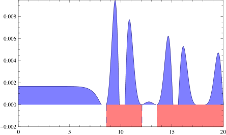
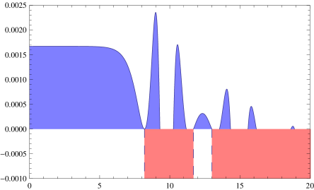
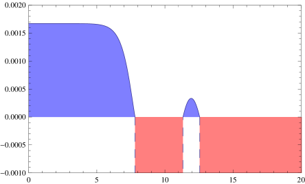
Figure 9: The Jacobi stability regions for the scalar field cosmological model with Higgs potential for different values of $\eta$: $\eta=10$ (top left), $\eta=20$ (top right), $\eta=30$ (bottom left) and $\eta=40$ (bottom right). The blue area shows the time intervals with $\chi>0$, and the black area shows the time intervals with $\kappa<0$. Where they overlap, both conditions $\chi>0$ and $\kappa<0$ are simultaneously satisfied, and the evolution is Jacobi stable.

In Figs. 10 we present the time variation of the components of the deviation vector $\xi^{i}$, $i=1,2$.

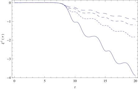
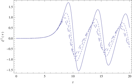
Figure 10: Time variations of the deviation vector components $\xi^{1}$ (left figure) and $\xi^{2}$ (right figure) for a Universe filled with a Higgs type scalar field, for different values of the parameter $\eta$: $\eta=10$ (solid curve), $\eta=20$ (dotted curve), $\eta=30$ (short dashed curve), and $\eta=40$ (dashed curve).

IV Jacobi stability analysis of the phantom quintessence and tachyonic cosmological models

In the present Section we will consider the Jacobi stability analysis of the standard dynamical system formulation of scalar field cosmological models. In this formulation the Friedmann equations are rewritten in the equivalent form of a three-dimensional first order dynamical system. Geometrically, we can describe the solutions of a first order dynamical system as a flow $\varphi_{t}:D\subset R^{n}\rightarrow R^{n}$, or, more generally, $\varphi_{t}:D\subset\mathcal{M}\rightarrow\mathcal{M}$, where $\mathcal{M}$ is a smooth $n$-dimensional manifold. The canonical lift of $\varphi_{t}$ to the tangent space $T\mathcal{M}$ is given by $\hat{\varphi}_{t}:T\mathcal{M}\rightarrow T\mathcal{M},\hat{\varphi}_{t}\left(u\right)=\left(\varphi_{t}\left(u\right),\dot{\varphi}_{t}\left(u\right)\right)$, where $\dot{\varphi}_{t}\left(u\right)=\frac{\partial\varphi\left(t,u\right)}{\partial t}$. Therefore, in order to apply the KCC theory to first order dynamical systems we must first lift the equations to the tangent bundle. Mathematically, this is equivalent to simply take the time derivative of the dynamical system.

IV.1 First order dynamical system formulation of quintessence and phantom quintessence scalar field cosmological models

In the following we assume that the energy density and pressure of the scalar field can be generally represented as

$$\rho_{\phi}=\zeta\frac{1}{2}\dot{\phi}^{2}+V(\phi),p_{\phi}=\zeta\frac{1}{2}\dot{\phi}^{2}-V(\phi),$$ (88)

where $\zeta=\pm 1$. The case $\zeta=+1$ corresponds to the quintessence fields, while $\zeta=-1$ describes the phantom scalar fields. We assume that the Universe is filled by ordinary matter with energy density $\rho_{m}$ and pressure $p_{m}$, and scalar fields. Each component of the model is characterized by their dimensionless density parameters $\Omega_{m}$ and $\Omega_{\phi}$, defined as

$$\Omega_{m}=\frac{\rho_{m}}{3H^{2}},\Omega_{\phi}=\frac{\rho_{\phi}}{3H^{2}},$$ (89)

and satisfying the constraint $\Omega_{m}+\Omega_{\phi}=1$. The cosmological equations describing this Universe model take the form

$$3H^{2}=\rho_{m}+\rho_{\phi},2\dot{H}=-\left(\rho_{m}+p_{m}+\rho_{\phi}+p_{\phi}\right),$$ (90)

and

$$\ddot{\phi}+3H\dot{\phi}+\zeta V^{\prime}(\phi)=0,$$ (91)

respectively. In the following we assume that the matter obeys a linear barotropic equation of state of the form $p_{m}=\left(\gamma_{m}-1\right)\rho_{m}$, where $\gamma_{m}$ is constant, and $1\leq\gamma_{m}\leq 2$. From the second Friedmann equation we immediately obtain the relation

$$-\frac{2\dot{H}}{H^{2}}=3\gamma_{m}\Omega_{m}+\zeta\frac{\dot{\phi}^{2}}{H^{2}}.$$ (92)

As basic variables in the first order dynamical description of cosmological dynamics we introduce the quantities $x$ and $y$, defined as

$$x=\frac{\dot{\phi}}{\sqrt{6}H},y=\frac{\sqrt{V}}{\sqrt{3}H}.$$ (93)

In these variables the density parameter of the scalar field is given by $\Omega_{\phi}=x^{2}+y^{2}$, while the density parameter of the matter can be written as $\Omega_{m}=1-\left(x^{2}+y^{2}\right)$. Moreover, the energy density and pressure of the scalar field are $p_{\phi}=3H^{2}\left(\zeta x^{2}+y^{2}\right)$ and $p_{\phi}=3H^{2}\left(\zeta x^{2}-y^{2}\right)$, respectively. Instead of the ordinary time variable $t$ we introduce the new independent variable $\tau$, defined as $\tau=\ln a(t)$, giving $d/dt=H\left(d/d\tau\right)$. Then, by taking the time derivative of $x$ and $y$ we obtain after some simple transformations cosm4

$$\frac{dx}{d\tau}=-3x(1-\zeta x^{2})+\frac{3\gamma_{m}}{2}x\left(1-x^{2}-y^{2}\right)-\sqrt{\frac{3}{2}}\zeta\frac{V^{\prime}}{V}y^{2},$$ (94)

$$\frac{dy}{d\tau}=\left[\frac{3\gamma_{m}}{2}\left(1-x^{2}-y^{2}\right)+3\zeta x^{2}\right]y+\sqrt{\frac{3}{2}}\frac{V^{\prime}}{V}xy.$$ (95)

The above system is not a closed system since one more equation involving $V^{\prime}/V$ is still lacking. Therefore we introduce a third variable $z$, defined as $z=V^{\prime}/V$. By taking its derivative with respect to the time $\tau$ we obtain

$$\frac{dz}{d\tau}=\sqrt{6}xz^{2}\left[\Gamma(z)-1\right],$$ (96)

where $\Gamma=VV^{\prime\prime}/V^{\prime 2}$. In order to lift this dynamical system to the tangent bundle we relabel the coordinates as

$$x=x^{1},y=x^{2},z=x^{3},y^{1}=\frac{dx^{1}}{d\tau},y^{2}=\frac{dx^{2}}{d\tau},y^{3}=\frac{dx^{3}}{d\tau}.$$ (97)

Then, by taking the derivatives with respect to $\tau$ of the first order cosmological dynamical system we obtain the equivalent second order system

$$\frac{d^{2}x^{1}}{d\tau^{2}}=-\frac{3}{2}\Bigg{\{}x^{\prime}\Bigg{(}-\gamma_{m}+3(\gamma_{m}-2\zeta)x^{2}+\gamma_{m}y^{2}+2\Bigg{)}-$$

$$y\Bigg{(}6\gamma_{m}xy^{\prime}+\sqrt{6}\zeta\left(2zy^{\prime}+yz^{\prime}\right)\Bigg{)}\Bigg{\}}=-2G^{1},$$

$$\frac{d^{2}x^{2}}{d\tau^{2}}=\frac{1}{2}\left[\sqrt{6}x^{2}x^{3}-6(\gamma_{m}-2\zeta)x^{1}x^{2}\right]y^{1}+$$

$$\frac{1}{2}\left[3\gamma_{m}-3(\gamma_{m}-2\zeta)\left(x^{1}\right)^{2}+\sqrt{6}x^{1}x^{3}-9\gamma_{m}\left(x^{2}\right)^{2}\right]y^{2}+$$

$$\sqrt{\frac{3}{2}}x^{1}x^{2}y^{3}=-2G^{2},$$ (99)

$$\frac{d^{2}x^{3}}{d\tau^{2}}=\sqrt{6}(x^{3})^{2}\left[\Gamma(x^{3})-1\right]y^{1}+\sqrt{6}x^{3}\Bigg{\{}x^{1}x^{3}\Gamma^{\prime}(x^{3})+$$

$$2x^{1}\left[\Gamma(x^{3})-1\right]\Bigg{\}}y^{3}=-2G^{3}.$$ (100)

The KCC geometric quantities (non-linear connection, deviation curvature tensor, and geodesic deviation equations) describing the Jacobi stability properties of the phantom quintessence cosmological model are presented in Appendix A.

IV.2 The phantom scalar field with power law potential

We assume that the potential of the phantom quintessence scalar field is given by a power law function, so that $V(\phi)=V_{0}\phi^{\alpha}$, where $\alpha$ is a constant. Then it follows immediately that $z=V^{\prime}/V=\alpha/\phi$, $\Gamma=(\alpha-1)/\alpha=\mathrm{constant}$, and $\Gamma^{\prime}(z)=0$. An important cosmological indicator is represented by the parameter of the total equation of state of the matter $w$, which for dust is defined as

$$w=\frac{p_{\phi}}{\rho_{\phi}+\rho_{m}}=\frac{\zeta x^{2}-y^{2}}{\left(\zeta-1\right)x^{2}+1}.$$ (101)

The variations of the density parameter of the phantom quintessence field $\Omega_{\phi}$ and of the parameter of the total equation of state are represented, as a function of the dust ($\gamma_{m}=1$) cosmological matter density parameter in Fig. 11. The initial conditions used to integrate the cosmological dynamical system are $x(0)=0.28$, $y(0)=0.47$, and $z(0)=0.1$, respectively.

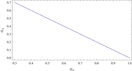
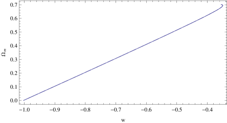
Figure 11: Variation of the density parameter of the phantom quintessence field as a function of the density parameter of the dust cosmological matter (left figure) and of the parameter $w$ of the total equation of state (right figure) for different values of $\alpha$: $\alpha=0.8$ (solid curve), $\alpha=1$ (dotted curve), $\alpha=1.2$ (short dashed curve), and $\alpha=1.4$ (dashed curve), respectively.

In this model the Universe starts its evolution in the large time limit from a matter dominated phase, with $\Omega_{m}=1$. During the cosmological expansion the role of the scalar field becomes dominant, and the Universe reaches the present day in a state of accelerated expansion, with $\Omega_{\phi}=0.75$, and $\Omega_{m}=0.25$, respectively. On the other hand, the de Sitter phase with $w=-1$ is reached only for vanishing ordinary matter density, when the Universe is fully dominated by the phantom quintessence field. It is also important to note that the cosmological evolution is basically independent on the numerical values of the exponent $\alpha$ in the scalar field potential.

The conditions of the Jacobi stability of the phantom quintessence cosmological model in its three-dimensional dynamic system representation are given by the four conditions that must be satisfied by the quantities $\left(\Sigma,\Phi,\Psi,\Omega\right)$, which are functions of the components of the deviation curvature tensor, and which are presented in Eqs. (26)-(II.4), for different values of $\alpha$. The time variations of $\left(\Sigma,\Phi,\Psi,\Omega\right)$ are represented in Fig. 12.

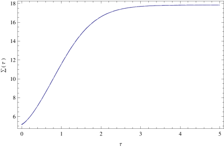
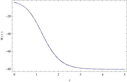
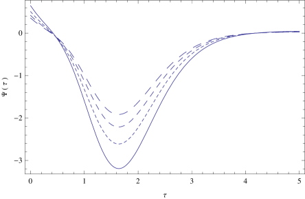
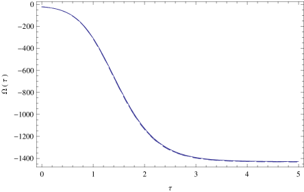
Figure 12: Time variation of the quantities $\left(\Sigma,\Phi,\Psi,\Omega\right)$, giving the Jacobi stability of the phantom quintessence field cosmological model with power law potential for different values of $\alpha$: $\alpha=0.8$ (solid curve), $\alpha=1$ (dotted curve), $\alpha=1.2$ (short dashed curve), and $\alpha=1.4$ (dashed curve), respectively.

As one can see from Fig. (12), the Jacobi stability condition $\Omega>0$ is not satisfied during the entire time evolution of this cosmological model. Therefore phantom quintessence scalar field cosmological models with power law potential are Jacobi unstable for all time intervals.

IV.3 Jacobi stability of tachyon field cosmological models

Tachyon scalar fields have been proposed as possible candidates to explain both inflation and the late acceleration of the Universe tach1 ; tach2 . It is also possible for the tachyonic field to trigger an the inflationary expansion, and at a later time generate a non-relativistic fluid, which could account for the existence of dark matter. A tachyonic scalar field is described by the Lagrangian $L=-V(\phi)\sqrt{1-\dot{\phi}^{2}}$, and it can be described in terms of an effective energy density and pressure, given by

$$\rho_{\phi}=\frac{V(\phi)}{\sqrt{1-\dot{\phi}^{2}}},p_{\phi}=-V(\phi)\sqrt{1-\dot{\phi}^{2}}.$$ (102)

The Friedmann equations are given by

$$3H^{2}=\rho_{m}+\frac{V(\phi)}{\sqrt{1-\dot{\phi}^{2}}},2\dot{H}+3H^{2}=-p_{m}+V(\phi)\sqrt{1-\dot{\phi}^{2}},$$ (103)

while the Klein-Gordon type equation satisfied by the scalar field is

$$\ddot{\phi}+3H\dot{\phi}\left(1-\dot{\phi}^{2}\right)+\frac{V^{\prime}(\phi)}{V(\phi)}\left(1-\dot{\phi}^{2}\right)=0.$$ (104)

The parameter of the equation of state of the tachyon field is given by

$$w=\frac{p_{\phi}}{\rho_{\phi}}=-\left(1-\dot{\phi}^{2}\right).$$ (105)

By adopting again for the matter the linear barotropic equation of state $p_{m}=\left(\gamma_{m}-1\right)\rho_{m}$, $1\leq\gamma_{m}\leq 2$, from the Friedmann equation we obtain first

$$\frac{2\dot{H}}{H^{2}}=-3\gamma_{m}\Omega_{m}-\frac{V(\phi)}{\sqrt{1-\dot{\phi}^{2}}}\frac{\dot{\phi}^{2}}{H^{2}}.$$ (106)

To formulate the cosmological evolution equation as a dynamical system we introduce a set of variables $(\tau,x,y,z)$ defined as

$$\tau=\ln a,x=\dot{\phi},y=\frac{\sqrt{V}}{\sqrt{3}H},z=\frac{V^{\prime}(\phi)}{V^{3/2}(\phi)}.$$ (107)

In these variables the density parameters of the scalar field and of the matter are given by

$$\Omega_{\phi}=\frac{y^{2}}{\sqrt{1-x^{2}}},\Omega_{m}=1-\frac{y^{2}}{\sqrt{1-x^{2}}}.$$ (108)

Then, by taking the derivative of $x$ and $y$ with respect to $\tau$ we obtain

$$\frac{dx}{d\tau}=-\sqrt{3}\left(1-x^{2}\right)\left(\sqrt{3}x+yz\right),$$ (109)

$$\frac{dy}{d\tau}=\frac{\sqrt{3}}{2}y\left\{xyz+\sqrt{3}\left[\gamma_{m}+\frac{y^{2}}{\sqrt{1-x^{2}}}\left(x^{2}-\gamma_{m}\right)\right]\right\},$$ (110)

$$\frac{dz}{d\tau}=\frac{3\sqrt{3}}{2}xyz^{2}\left[\Gamma(z)-1\right],$$ (111)

where $\Gamma(z)=(2/3)VV^{\prime\prime}/V^{\prime}{{}^{2}}$. By lifting the cosmological field equations to the tangent bundle we obtain

$$\frac{d^{2}x}{d\tau^{2}} = 2\sqrt{3}xx^{\prime}\left(\sqrt{3}x+yz\right)-\sqrt{3}\left(1-x^{2}\right)\Bigg{(}\sqrt{3}x^{\prime}+$$ (112)

$$y^{\prime}z+yz^{\prime}\Bigg{)}=-2G^{1},$$

$$\frac{d^{2}y}{d\tau^{2}} = \frac{\sqrt{3}}{2}\Bigg{\{}3y\Bigg{[}\gamma_{m}\left(-\frac{xy^{2}x^{\prime}}{\left(1-x^{2}\right)^{3/2}}-\frac{2yy^{\prime}}{\sqrt{1-x^{2}}}\right)$$ (113)

$$+2xy^{2}x^{\prime 2}yy^{\prime}\Bigg{]}+y^{2}zx^{\prime}+3y^{\prime}\times$$

$$\Bigg{[}\gamma_{m}\left(1-\frac{y^{2}}{\sqrt{1-x^{2}}}\right)+x^{2}y^{2}\Bigg{]}+$$

$$2xyzy^{\prime 2}z^{\prime}\Bigg{\}}=-2G^{2},$$

$$\frac{d^{2}z}{d\tau^{2}} = \frac{3}{2}\sqrt{3}z\Bigg{\{}(\Gamma(z)-1)\left[y\left(zx^{\prime}+2xz^{\prime}\right)+xzy^{\prime}\right]+$$ (114)

$$xyzz^{\prime}\Gamma^{\prime}(z)\Bigg{\}}=-2G^{3}.$$

The KCC geometric quantities (non-linear connection, deviation curvature tensor, and geodesic deviation equations) describing the Jacobi stability properties of the tachyon scalar field cosmological model are presented in Appendix B.

IV.3.1 Power law potential tachyonic scalar field cosmological models

In the following we assume again that the potential of the tachyonic scalar field is power law type, with $V(\phi)=V_{0}\phi^{\alpha}$, where $V_{0}$ and $\alpha$ are constants. This choice immediately gives $\Gamma=(2/3)\left(\alpha-1\right)/\alpha$. The parametric dependence of the density parameter $\Omega_{\phi}$ of the tachyonic scalar field with power law potential on the matter energy density $\Omega_{m}$ is represented in the left panel of Fig. 13. The parametric variation of the matter density parameter $\Omega_{m}$ as a function of the parameter of the total equation of state of matter $w$ is shown in the right panel of Fig. 13.

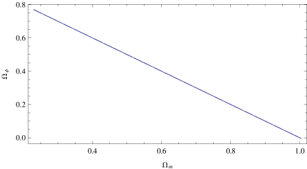
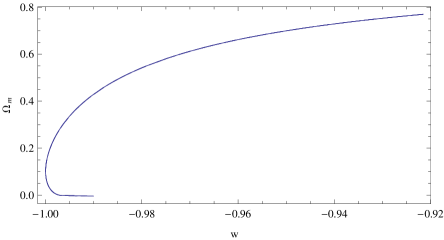
Figure 13: Variation of the density parameter of the tachyonic scalar field with power law potential as a function of the density parameter of the dust cosmological matter ($\gamma_{m}=1$) (left figure) and of the parameter $w$ of the total equation of state (right figure) for different values of $\alpha$: $\alpha=0.8$ (solid curve), $\alpha=1$ (dotted curve), $\alpha=1.2$ (short dashed curve), and $\alpha=1.4$ (dashed curve), respectively.

In order to numerically integrate the dynamical system corresponding to the tachyon scalar field model we have used the initial conditions $x(0)=0.28$, $y(0)=0.45$, and $z(0)=0.1$, respectively, and we have assumed that the ordinary matter in the Universe is in the form of zero pressure dust, with $\gamma_{m}=1$. There is a linear relation between $\Omega_{\phi}$ and $\Omega_{m}$. The Universe starts its cosmological evolution in a matter dominated phase, with $\Omega_{m}=1$, $\Omega_{\phi}=0$, with decelerating expansion. The energy density of the tachyon field increases in time, and the Universe enters in a de Sitter phase, with the matter density becoming negligibly small. The parameter of the total equation of state satisfies the condition $w<0$ during the entire cosmological evolution. It is also interesting to note that the time evolution of this model is basically independent on the numerical values of the exponent $\alpha$ in the power law potential. The time variations of $\left(\Sigma,\Phi,\Psi,\Omega\right)$ describing the Jacobi stability of the tachyon scalar field cosmological model are represented in Fig. 14.

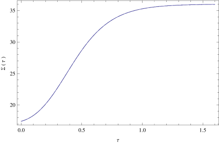
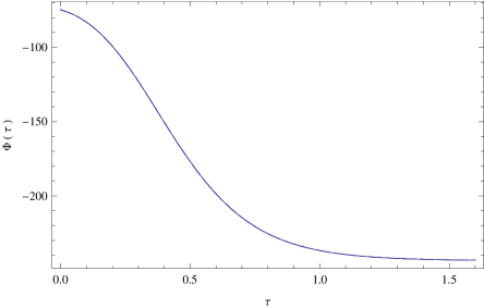
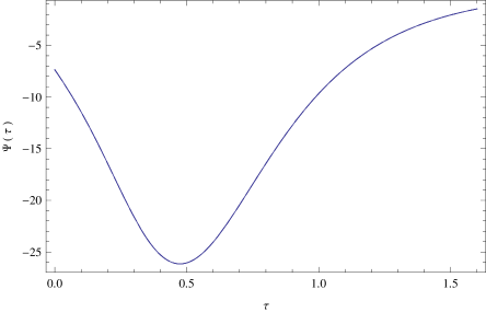
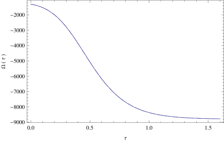
Figure 14: Time variation of the quantities $\left(\Sigma,\Phi,\Psi,\Omega\right)$, giving the Jacobi stability of the tachyon scalar field cosmological model with power law potential for different values of $\alpha$: $\alpha=0.8$ (solid curve), $\alpha=1$ (dotted curve), $\alpha=1.2$ (short dashed curve), and $\alpha=1.4$ (dashed curve), respectively.

As one can see from Fig. (14), the Jacobi stability condition $\Omega>0$ is not satisfied during the entire cosmological evolution period of this scalar field model. Therefore it follows that tachyon scalar field cosmological models with power law potential are Jacobi unstable for all time intervals. This result is independent on the numerical values of the exponent $\alpha$ in the tachyon scalar field potential.

V Discussions and final remarks

In the present paper we have investigated the Jacobi stability properties of the scalar field cosmological models by using the KCC theory, which represents a powerful mathematical method for the analysis of dynamical systems. Scalar field cosmological models represent a non-trivial testing object for studying non-linear effects in the framework of general relativity. From a mathematical point of view the Jacobi (in)stability represents a natural generalization of the (in)stability of the geodesic flow on a differentiable manifold, endowed with a Riemannian or Finslerian type metric to a non-metric setting. The KCC theory can be applied to scalar field cosmological models that can be formulated mathematically as sets of second order ordinary non-linear differential equations. Then the geometric invariants associated to this system (nonlinear and Berwald connections), and the deviation curvature tensor, as well as its eigenvalues, can be explicitly obtained. The time evolution of the components of the deviation vector can also be obtained by explicitly solving the geodesic deviation equations.

The Jacobi stability, and its theoretical foundation, the KCC theory, offers an alternative approach to the ”classical” Lyapunov approach, by investigating the deviations of the entire trajectory of the cosmological evolution equations with respect to the nearby ones under the effects of a small perturbation. In the framework of general relativity we may call the applications of the KCC theory to the study of the gravitational fields as a ”second geometrization”, in which already geometric quantities are supplemented by additional geometric structures. Hence general relativistic cosmological models can be described in geometric terms originating from their dynamical system structure, with these new geometric structure fully determined by the underlying Riemannian geometry, and the physical properties of the scalar fields (their self-interaction potential). The stability properties of the perturbations of a given trajectory describing the cosmological evolution are determined by the properties of the curvature deviation tensor, a geometric quantity constructed from the connections (non-linear and Berwald) associated to the dynamical system describing the cosmological evolution. It is important to note that the KCC theory can be directly applied to systems of second order differential equations, which can be interpreted geometrically as the paths (or geodesics) associated to a semispray. In investigating the Jacobi stability of cosmological models we have followed two approaches. Since the cosmological evolution equations (the Friedmann equations) are second order differential equations, the KCC theory can be naturally and directly applied to study the stability of the cosmic evolution. As a first step one obtains the two non-zero components of the non-linear connection, with the $N_{2}^{1}$ component depending on the product of the scale factor and of the time derivative of the field, while the $N_{2}^{2}$ component depends on the energy density of the scalar field, as well as of the scalar field potential. After obtaining the components of the deviation curvature tensor we have formulated the general condition of the stability of the scalar field cosmological models, which is determined by two inequalities involving the second and the first derivative of the scalar field potential, the energy density of the field, and the time variation of the scalar field itself.

As an applications of the developed formalism we have considered two scalar field models, both being relevant for the study of both the early and the late stages of the cosmological evolution. The first case we did consider is the scalar field with exponential potential. We have studied in detail the KCC geometric properties of this model. It turns out that the Jacobi stability condition, which can be expressed in terms of the components of the deviation curvature tensor is not satisfied during the cosmological evolution, and that the Universe described by the exponential potential scalar field is in a Jacobi unstable state. This result is independent on the numerical values of the parameter $\lambda$, describing the properties of the potential, and can also be inferred from the behavior of the components of the deviation vector $\xi^{i}$, with $\xi^{1}$ diverging exponentially in time. As a second case we have considered the case of the Higgs type potential. For this potential the KCC geometric quantities show a complex behavior. After a period in which the scalar field and the potential are almost constant, the field starts to oscillate, with the amplitude of the oscillations decreasing in time. This behavior of the Higgs field is also reflected in the behavior of the components of the deviation curvature tensor, which are also some oscillating functions. The Jacobi stability of this cosmological model strongly depends on the numerical value of the parameter $\eta=\lambda/4M^{2}$. For small values of $\eta$, the Universe evolves between successive Jacobi stable and unstable states. With the increase of the numerical value of $\eta$ the time intervals in which the Universe is Jacobi stable decrease quickly, and for large values of $\eta$ the Universe is in a Jacobi unstable state during its entire cosmological evolution.

As a second approach for the study of the Jacobi stability of scalar field cosmologies we have considered the first order dynamical system formulation of scalar field evolution equations. In this approach by introducing a new set of variables, expressed in terms of the square root of the potential, the time derivative of the scalar field, and the Hubble function, respectively, the Friedmann equations in the presence of scalar fields can be reformulated as a first order dynamical system, consisting of three highly non-linear ordinary differential equations. In order to apply the KCC theory this dynamical system must be lifted to the tangent bundle, and formulated as a second order differential system. We have analyzed, by using this approach, two specific scalar field models, the phantom quintessence and the tachyon scalar field with power law potentials. It turns out that for this choice of the potential both scalar field models are Jacobi unstable. The power law potential gives a very simple form for the function $\Gamma(z)$, which takes constant values during the cosmological evolution. This situation is similar to the case of the exponential potential, and leads to a significant simplification of the mathematical formalism.

We have started our study of the applications of the KCC theory to cosmological problems with the investigation of the standard mater dominated cosmological models in their dynamical system formulation. We have studied the Jacobi stability of the critical points of different models, and we have shown that they are Jacobi unstable. A full comparison between the Jacobi and Lyapunov properties of the critical points for second order systems was given in Sa05 and Sa05a , and hence we will not discuss in detail this relation. However, this study of the critical points of matter dominated cosmological models also shows the fundamental differences between the Lyapunov stability and KCC theories: while Lypunov stability is mostly restricted to the study of critical points, the KCC theory has the potential of investigating the deviation of the full trajectory during the entire period of the cosmological evolution. Therefore we can consider a Lyapunov stability analysis of steady states (called the linear analysis), and a ”Lyapunov type” stability analysis of the whole trajectory (the KCC or Jacobi stability analysis), and these two methods are complementary but distinct to each other.

The KCC theory also introduces the first set of KCC invariants $\epsilon^{i}$, $i=1,...,n$, giving the contravariant KCC derivative of the vector field $y^{i}$. The first KCC invariant can be interpreted as an external force. We did not study in detail the time evolution of the first KCC invariant, since its properties are not directly related to the stability issues that were our main points of interest.

In the present paper we have performed a stability analysis of the scalar field cosmological models, in which we have considered a description of the deviations of the whole trajectories of the differential system describing the cosmological dynamics, and we have provided some basic theoretical and computational tools for this study. Further investigations of the Jacobi stability properties of cosmological models may provide some methods for discriminating between different evolutionary scenarios, as well as for the better understanding of some other fundamental processes, like, for example, structure formation, that played an essential role in the evolution of our Universe.

Conflict of interest

The authors declare that there is no conflict of interest regarding the publication of this paper.

Appendix A The non-linear connection, the curvature deviation tensor and the geodesic deviation equations for the phantom quintessence scalar field cosmological model

The coefficients of the non-linear connection associated to the dynamical system describing the phantom quintessence cosmological model are given by

$$N_{1}^{1} = -3\gamma_{m}x^{2}+6\zeta x^{2}-3\left(1-\zeta x^{2}\right)+$$

$$\frac{3}{2}\gamma_{m}\left(-x^{2}-y^{2}+1\right),$$

$$N_{1}^{2}=-3\gamma_{m}xy-\sqrt{6}\zeta yz,\;\;N_{1}^{3}=-\sqrt{\frac{3}{2}}\zeta y^{2},$$

$$N_{2}^{1}=y(6\zeta x-3\gamma_{m}x)+\sqrt{\frac{3}{2}}yz,$$

$$N_{2}^{2} = 3\zeta x^{2}+\frac{3}{2}\gamma_{m}\left(-x^{2}-y^{2}+1\right)+\sqrt{\frac{3}{2}}xz-3\gamma_{m}y^{2},$$

$$N_{2}^{3}=\sqrt{\frac{3}{2}}xy,N_{3}^{1}=\sqrt{6}z^{2}\left[\Gamma(z)-1\right],N_{3}^{2}=0,$$

$$N_{3}^{3}=\sqrt{6}xz^{2}\Gamma^{\prime}(z)+2\sqrt{6}xz\left[\Gamma(z)-1\right].$$

The first KCC invariants $\epsilon^{i}$, $i=1,2,3$ are given by

$$\epsilon^{1} = \frac{3}{2}\Bigg{\{}x^{\prime}\left(\gamma_{m}-3(\gamma_{m}-2\zeta)x^{2}-\gamma_{m}y^{2}-2\right)-$$

$$y\left(6\gamma_{m}xy^{\prime}+\sqrt{6}\zeta\left(2zy^{\prime}+yz^{\prime}\right)\right)\Bigg{\}},$$

$$\epsilon^{2} = \frac{1}{2}\Bigg{\{}x\left(\sqrt{6}\left(zy^{\prime}+yz^{\prime}\right)-6(\gamma_{m}-2\zeta)yx^{\prime}\right)+$$

$$\sqrt{6}yzx^{\prime}-3(\gamma_{m}-2\zeta)x^{2}y^{\prime}-9\gamma_{m}y^{2}y^{\prime}+3\gamma_{m}y^{\prime}\Bigg{\}},$$

$$\epsilon^{3}=\sqrt{6}z\left((\Gamma(z)-1)\left(zx^{\prime}+2xz^{\prime}\right)+xzz^{\prime}\Gamma^{\prime}(z)\right).$$

All Berwald connection components are zero here.
The components of the curvature deviation tensor are

$$P_{1}^{1} = \frac{1}{4}\Bigg{\{}9\left(4(\gamma_{m}-2\zeta)xx^{\prime}+\left(\gamma_{m}-3(\gamma_{m}-2\zeta)x^{2}-2\right)^{2}\right)+$$

$$6y^{2}\Bigg{(}-3(\gamma_{m}-2)\gamma_{m}+15\gamma_{m}(\gamma_{m}-2\zeta)x^{2}-$$

$$\sqrt{6}\left(-2\gamma_{m}\zeta+\gamma_{m}+4\zeta^{2}\right)xz-2\zeta z^{2}\Gamma(z)\Bigg{)}+$$

$$12\gamma_{m}yy^{\prime}+9\gamma_{m}^{2}y^{4}\Bigg{\}},$$

$$P_{1}^{2} = 3\gamma_{m}yx^{\prime}+3x\Bigg{[}\gamma_{m}y^{\prime}+6\gamma_{m}^{2}y^{3}-y\Bigg{(}3(\gamma_{m}-1)\gamma_{m}+$$

$$\zeta z^{2}\Bigg{)}\Bigg{]}+18\gamma_{m}(\gamma_{m}-2\zeta)x^{3}y+$$

$$3\sqrt{\frac{3}{2}}\left(-4\gamma_{m}\zeta+\gamma_{m}+8\zeta^{2}\right)x^{2}yz+$$

$$\sqrt{6}\zeta\left(z\left(y^{\prime}+6\gamma_{m}y^{3}-3(\gamma_{m}-1)y\right)+yz^{\prime}\right),$$

$$P_{1}^{3} = \frac{1}{2}\sqrt{\frac{3}{2}}y\Bigg{\{}-y\Bigg{[}3(\gamma_{m}-2)\zeta+\left(-9\gamma_{m}\zeta+6\gamma_{m}+18\zeta^{2}\right)\times$$

$$x^{2}+2\sqrt{6}\zeta xz\left(z\Gamma^{\prime}(z)+2\Gamma(z)-1\right)\Bigg{]}+$$

$$4\zeta y^{\prime}+3\gamma_{m}\zeta y^{3}\Bigg{\}},$$

$$P_{2}^{1} = \frac{1}{2}\Bigg{\{}y\Bigg{[}6(\gamma_{m}-2\zeta)x^{\prime}+36(\gamma_{m}-2\zeta)^{2}x^{3}-$$

$$3x\left(6(\gamma_{m}-1)(\gamma_{m}-2\zeta)+z^{2}(1-2\Gamma(z))\right)-$$

$$9\sqrt{6}(\gamma_{m}-2\zeta)x^{2}z-\sqrt{6}z^{\prime}+3\sqrt{6}(\gamma_{m}-1)z\Bigg{]}+$$

$$y^{\prime}\left(6(\gamma_{m}-2\zeta)x-\sqrt{6}z\right)+$$

$$6\gamma_{m}y^{3}\left(6(\gamma_{m}-2\zeta)x-\sqrt{6}z\right)\Bigg{\}},$$

$$P_{2}^{2} = \frac{1}{4}\Bigg{\{}2x\Bigg{[}6(\gamma_{m}-2\zeta)x^{\prime}+3\sqrt{6}z\times$$

$$\left(\gamma_{m}+2\left(\gamma_{m}(\zeta-2)-2\zeta^{2}\right)y^{2}\right)-\sqrt{6}z^{\prime}\Bigg{]}-2\sqrt{6}zx^{\prime}+$$

$$9(\gamma_{m}-2\zeta)^{2}x^{4}+6x^{2}\left(3\gamma_{m}(\gamma_{m}-2\zeta)\left(5y^{2}-1\right)+z^{2}\right)-$$

$$6\sqrt{6}(\gamma_{m}-2\zeta)x^{3}z+9\gamma_{m}\left(4yy^{\prime}+\gamma_{m}\left(1-3y^{2}\right)^{2}\right)-$$

$$12\zeta y^{2}z^{2}\Bigg{\}},$$

$$P_{2}^{3} = -\frac{1}{2}\sqrt{\frac{3}{2}}\Bigg{\{}(y\Bigg{[}2x^{\prime}+3(\gamma_{m}-2\zeta)x^{3}-3\gamma_{m}x+$$

$$\sqrt{6}x^{2}z\left(-2z\Gamma^{\prime}(z)-4\Gamma(z)+3\right)\Bigg{]}+2xy^{\prime}$$

$$+y^{3}\left(\left(\gamma_{m}(9-6\zeta)+12\zeta^{2}\right)x+\sqrt{6}\zeta z\right)\Bigg{\}},$$

$$P_{3}^{1} = \sqrt{\frac{3}{2}}z\Bigg{\{}z\Bigg{[}-3(\Gamma(z)-1)\Bigg{(}-\gamma_{m}+3(\gamma_{m}-2\zeta)x^{2}$$

$$+\gamma_{m}y^{2}+2\Bigg{)}-2z^{\prime}\Gamma^{\prime}(z)\Bigg{]}+2\sqrt{6}xz^{3}\times$$

$$(\Gamma(z)-1)\Gamma^{\prime}(z)+4\sqrt{6}xz^{2}(\Gamma(z)-1)^{2}-$$

$$4(\Gamma(z)-1)z^{\prime}\Bigg{\}},$$

$$P_{3}^{2}=-3yz^{2}(\Gamma(z)-1)\left(\sqrt{6}\gamma_{m}x+2\zeta z\right),$$

$$P_{3}^{3} = -z\left(\sqrt{6}x^{\prime}\left(z\Gamma^{\prime}(z)+2\Gamma(z)-2\right)+3\zeta y^{2}z(\Gamma(z)-1)\right)-$$

$$\sqrt{6}xz^{\prime}\left(z^{2}\Gamma^{\prime\prime}(z)+4z\Gamma^{\prime}(z)+2\Gamma(z)-2\right)+$$

$$6x^{2}z^{2}\left(z\Gamma^{\prime}(z)+2\Gamma(z)-2\right)^{2}.$$

The geodesic deviation equations are obtained in the form

$$\frac{d^{2}\xi^{1}}{d\tau^{2}}+\xi^{1}\left(-18(\gamma_{m}-2\zeta)xx^{\prime}-6\gamma_{m}yy^{\prime}\right)-$$

$$2\xi^{2}\left(y\left(3\gamma_{m}x^{\prime}+\sqrt{6}\zeta z^{\prime}\right)+y^{\prime}\left(3\gamma_{m}x+\sqrt{6}\zeta z\right)\right)+$$

$$\frac{\xi^{1}}{d\tau}\left(3\gamma_{m}-9(\gamma_{m}-2\zeta)x^{2}-3\gamma_{m}y^{2}-6\right)-$$

$$2\frac{\xi^{2}}{d\tau}y\left(3\gamma_{m}x+\sqrt{6}\zeta z\right)-2\sqrt{6}\zeta\xi^{3}yy^{\prime}-\sqrt{6}\zeta\frac{\xi^{3}}{d\tau}y^{2}=0,$$

$$\frac{d^{2}\xi^{2}}{d\tau^{2}}+\sqrt{6}\xi^{3}\left(yx^{\prime}+xy^{\prime}\right)+\xi^{1}\times$$

$$\left(y\left(\sqrt{6}z^{\prime}-6(\gamma_{m}-2\zeta)x^{\prime}\right)+y^{\prime}\left(\sqrt{6}z-6(\gamma_{m}-2\zeta)x\right)\right)+$$

$$\xi^{2}\left(x^{\prime}\left(\sqrt{6}z-6(\gamma_{m}-2\zeta)x\right)+\sqrt{6}xz^{\prime}-18\gamma_{m}yy^{\prime}\right)+$$

$$\sqrt{6}\frac{\xi^{3}}{d\tau}xy+\frac{\xi^{1}}{d\tau}y\left(\sqrt{6}z-6(\gamma_{m}-2\zeta)x\right)+$$

$$\frac{\xi^{2}}{d\tau}\left(3\gamma_{m}-3(\gamma_{m}-2\zeta)x^{2}+\sqrt{6}xz-9\gamma_{m}y^{2}\right)=0,$$

$$\frac{d^{2}\xi^{3}}{d\tau^{2}}+2\sqrt{6}\xi^{3}\Bigg{(}zx^{\prime}\left(z\Gamma^{\prime}(z)+2\Gamma(z)-2\right)+$$

$$xz^{\prime}\left(z^{2}\Gamma^{\prime\prime}(z)+4z\Gamma^{\prime}(z)+2\Gamma(z)-2\right)\Bigg{)}+$$

$$2\sqrt{6}\frac{\xi^{3}}{d\tau}xz\left(z\Gamma^{\prime}(z)+2\Gamma(z)-2\right)+2\sqrt{6}\times$$

$$\xi^{1}zz^{\prime}\left(z\Gamma^{\prime}(z)+2\Gamma(z)-2\right)+2\sqrt{6}\frac{\xi^{1}}{d\tau}z^{2}(\Gamma(z)-1)=0.$$

Appendix B The non-linear connection, the curvature deviation tensor and the geodesic deviation equations for the tachyon scalar field cosmological model

The coefficients of the non-linear connection associated to the dynamical system describing the tachyon scalar field cosmological model are given by

$$N_{1}^{1}=2\sqrt{3}x\left(\sqrt{3}x+y\right)-3\left(1-x^{2}\right),$$

$$N_{1}^{2}=-\sqrt{3}\left(1-x^{2}\right)z,\;N_{1}^{3}=-\sqrt{3}\left(1-x^{2}\right)y,$$

$$N_{2}^{1}=\frac{\sqrt{3}}{2}\left(3y\left(2xy^{2}-\frac{\gamma_{m}xy^{2}}{\left(1-x)^{2}\right)^{3/2}}\right)+y^{2}z\right),$$

$$N_{2}^{2} = \frac{\sqrt{3}}{2}\Bigg{\{}3\left(2x^{2}y-\frac{2\gamma_{m}y}{\sqrt{1-x^{2}}}\right)+$$

$$3\Bigg{[}\gamma_{m}\left(1-\frac{y^{2}}{\sqrt{1-x^{2}}}\right)+x^{2}y^{2}\Bigg{]}+2xyz\Bigg{\}},$$

$$N_{2}^{3}=\frac{1}{2}\sqrt{3}xy^{2},\;N_{3}^{1}=\frac{3}{2}\sqrt{3}yz^{2}(\Gamma(z)-1),$$

$$N_{3}^{2}=\frac{3}{2}\sqrt{3}xz^{2}(\Gamma(z)-1),$$

$$N_{3}^{3} = \frac{3}{2}\sqrt{3}xyz^{2}\Gamma^{\prime}(z)+3\sqrt{3}xyz(\Gamma(z)-1).$$

The first KCC invariants $\epsilon^{i}$, $i=1,2,3$ are

$$\epsilon^{1} = x^{\prime}\left(9x^{2}+2\sqrt{3}xyz-3\right)+\sqrt{3}\left(x^{2}-1\right)\left(zy^{\prime}+yz^{\prime}\right),$$

$$\epsilon^{2} = \frac{1}{2\left(x^{2}-1\right)^{2}}\Bigg{\{}\sqrt{3}\Bigg{[}-3\gamma_{m}x\sqrt{1-x^{2}}y^{3}x^{\prime}+$$

$$\left(x^{2}-1\right)^{2}y^{2}x^{\prime}(6xy+z)+9\gamma_{m}x^{2}\sqrt{1-x^{2}}y^{2}y^{\prime}-$$

$$9\gamma_{m}\sqrt{1-x^{2}}y^{2}y^{\prime}+\left(x^{2}-1\right)^{2}\times$$

$$\left(y^{\prime}(3\gamma_{m}+xy(9xy+2z))+xy^{2}z^{\prime}\right)\Bigg{]}\Bigg{\}},$$

$$\epsilon^{3}=\frac{3}{2}\sqrt{3}z\left\{(\Gamma(z)-1)\left[y\left(zx^{\prime}+2xz^{\prime}\right)+xzy^{\prime}\right]+xyzz^{\prime}\Gamma^{\prime}(z)\right\}.$$

All Berwald connection components are zero here. The components of the curvature deviation tensor are

$$P_{1}^{1} = x\Bigg{[}-2\left(9x^{\prime}+\sqrt{3}zy^{\prime}\right)+\frac{9}{2}y^{3}z\left(\frac{\gamma_{m}}{\sqrt{1-x^{2}}}-2\right)$$

$$-2\sqrt{3}y\left(z^{\prime}+6z\right)\Bigg{]}-\frac{1}{2}yz\left(4\sqrt{3}x^{\prime}+3yz(3\Gamma(z)-2)\right)$$

$$+81x^{4}+\frac{9}{2}x^{2}\left(y^{2}z^{2}(\Gamma(z)+2)-12\right)$$

$$+9x^{3}y\left(y^{2}+4\sqrt{3}\right)z+9,$$

$$P_{1}^{2} = \frac{1}{2}\Bigg{\{}z\Bigg{[}-9\gamma_{m}-4\sqrt{3}xx^{\prime 2}\left(-3\gamma_{m}+9y^{2}+8\sqrt{3}\right)$$

$$+27\gamma_{m}\sqrt{1-x^{2}}y^{2}+9x^{4}\left(3y^{2}+2\sqrt{3}\right)+6\sqrt{3}\Bigg{]}$$

$$+9x\left(x^{2}-1\right)yz^{2}(\Gamma(z)+1)-2\sqrt{3}\left(x^{2}-1\right)z^{\prime}\Bigg{\}},$$

$$P_{1}^{3} = \sqrt{3}y\left(-2xx^{\prime 4}-12x^{2}+3\right)-\sqrt{3}\left(x^{2}-1\right)y^{\prime}$$

$$+\frac{3}{2}x\left(x^{2}-1\right)y^{2}z\left(3z\Gamma^{\prime}(z)+6\Gamma(z)-1\right),$$

$$P_{2}^{1} = \frac{1}{4}y\Bigg{\{}6\sqrt{3}y^{2}\left(\frac{\gamma_{m}}{\left(1-x^{2}\right)^{5/2}}-2\right)x^{\prime 2}y$$

$$\times\left(\frac{4\sqrt{3}\gamma_{m}yx^{\prime}}{\left(1-x^{2}\right)^{5/2}}+\left(45y^{2}+6\sqrt{3}\right)z\right)$$

$$+\frac{1}{\left(1-x^{2}\right)^{5/2}}\Bigg{[}9x^{3}y\Bigg{(}18\left(1-x^{2}\right)^{5/2}y^{3}+12\sqrt{3}$$

$$\times\left(1-x^{2}\right)^{5/2}y-2\sqrt{3}\gamma_{m}y^{\prime}+3\gamma_{m}^{2}y+27\gamma_{m}y^{3}$$

$$-8\sqrt{3}\gamma_{m}y\Bigg{)}\Bigg{]}+9xy\Bigg{[}2\sqrt{3}\left(\frac{\gamma_{m}}{\left(1-x^{2}\right)^{5/2}}-2\right)y^{\prime}$$

$$+\frac{9\gamma_{m}y^{3}\left(\gamma_{m}\sqrt{1-x^{2}}-2\right)}{\left(1-x^{2}\right)^{5/2}}+y$$

$$\times\Bigg{(}\frac{\left(2\sqrt{3}-3\gamma_{m}\right)\left(\gamma_{m}-2\left(1-x^{2}\right)^{5/2}\right)}{\left(1-x^{2}\right)^{5/2}}$$

$$+z^{2}(\Gamma(z)+1)\Bigg{)}\Bigg{]}+\frac{27\gamma_{m}x^{5}y^{2}\left(2\sqrt{3}-3y^{2}\right)}{\left(1-x^{2}\right)^{5/2}}$$

$$+\frac{27\gamma_{m}x^{4}y^{3}z}{\left(1-x^{2}\right)^{5/2}}-\frac{27\gamma_{m}y^{3}z}{\left(1-x^{2}\right)^{5/2}}-4\sqrt{3}zy^{\prime}$$

$$+y\left(9\gamma_{m}z-2\sqrt{3}\left(z^{\prime}+3z\right)\right)\Bigg{\}},$$

$$P_{2}^{2} = \frac{1}{4\left(x^{2}-1\right)^{2}}\Bigg{\{}-4\left(x^{2}-1\right)^{2}y\Bigg{[}z\left(\sqrt{3}x^{\prime}-9\gamma_{m}x\right)$$

$$+\sqrt{3}x\left(9xy^{\prime}+z^{\prime}\right)\Bigg{]}+18\gamma_{m}x\sqrt{3-3x^{2}}y^{2}x^{\prime}$$

$$+3\left(x^{2}-1\right)^{2}y^{2}\Bigg{[}3x\left(x\left(18\gamma_{m}+z^{2}(\Gamma(z)+1)\right)-4\sqrt{3}x^{\prime}\right)$$

$$-2z^{2}\Bigg{]}-36\gamma_{m}x^{2}\sqrt{3-3x^{2}}yy^{\prime}+36\gamma_{m}\sqrt{3-3x^{2}}yy^{\prime}$$

$$+\left(x^{2}-1\right)^{2}\left(27\gamma_{m}^{2}-4\sqrt{3}xzy^{\prime}\right)$$

$$-243\left(x^{2}-1\right)y^{4}\left(\gamma_{m}^{2}-x^{6}+x^{4}\right)$$

$$-162\gamma_{m}^{2}\sqrt{1-x^{2}}y^{2}+162\gamma_{m}^{2}x^{2}\sqrt{1-x^{2}}y^{2}$$

$$+486\gamma_{m}x^{4}\sqrt{1-x^{2}}y^{4}-486\gamma_{m}x^{2}\sqrt{1-x^{2}}y^{4}$$

$$+90\gamma_{m}x^{3}\sqrt{1-x^{2}}y^{3}z-90\gamma_{m}x\sqrt{1-x^{2}}y^{3}z$$

$$+36x\left(x^{2}-1\right)^{2}\left(4x^{2}-1\right)y^{3}z\Bigg{\}},$$

$$P_{2}^{3} = \frac{1}{4}y\Bigg{\{}y\left(9\gamma_{m}x-2\sqrt{3}x^{\prime}\right)-4\sqrt{3}xy^{\prime}$$

$$-\frac{9\gamma_{m}xy^{3}}{\sqrt{1-x^{2}}}+9x\left(7x^{2}-4\right)y^{3}$$

$$+3y^{2}z\left(x^{2}\left(3z\Gamma^{\prime}(z)+6\Gamma(z)-2\right)-2\right)\Bigg{\}},$$

$$P_{3}^{1} = -\frac{1}{4\left(1-x^{2}\right)^{3/2}}\Bigg{\{}3z\Bigg{[}-2\sqrt{3-3x^{2}}\left(x^{2}-1\right)$$

$$\times zy^{\prime}(\Gamma(z)-1)+2\sqrt{3-3x^{2}}\left(x^{2}-1\right)y\Bigg{(}(\Gamma(z)-1)$$

$$\times\left(\left(9x^{2}-3\right)z-2z^{\prime}\right)-zz^{\prime}\Gamma^{\prime}(z)\Bigg{)}$$

$$-3x\left(1-x^{2}\right)^{3/2}y^{2}z^{2}(\Gamma(z)-1)\Bigg{(}3z\Gamma^{\prime}(z)$$

$$+6\Gamma(z)-1\Bigg{)}+9x^{2}y^{3}z\Bigg{(}\gamma_{m}+2\sqrt{1-x^{2}}x^{2}$$

$$-2\sqrt{1-x^{2}}\Bigg{)}(\Gamma(z)-1)\Bigg{]}\Bigg{\}},$$

$$P_{3}^{2} = \frac{1}{4\sqrt{1-x^{2}}}\Bigg{\{}3z\Bigg{[}-2\sqrt{1-x^{2}}z(\Gamma(z)-1)$$

$$\times\left(\sqrt{3}x^{\prime}+3yz\right)+x\Bigg{(}z\Bigg{(}\sqrt{1-x^{2}}$$

$$\times\left(-9\gamma_{m}-2\sqrt{3}z^{\prime}\Gamma^{\prime}(z)+9\gamma_{m}\Gamma(z)\right)$$

$$-27\gamma_{m}y^{2}(\Gamma(z)-1)\Bigg{)}-4\sqrt{3-3x^{2}}(\Gamma(z)-1)z^{\prime}\Bigg{)}$$

$$+3\sqrt{1-x^{2}}x^{2}yz^{2}(\Gamma(z)-1)\left(3z\Gamma^{\prime}(z)+6\Gamma(z)-2\right)$$

$$+27\sqrt{1-x^{2}}x^{3}y^{2}z(\Gamma(z)-1)\Bigg{]}\Bigg{\}},$$

$$P_{3}^{3} = \frac{3}{4}\Bigg{\{}-2\sqrt{3}y\Bigg{(}2z\left(x^{\prime}(\Gamma(z)-1)+2xz^{\prime}\Gamma^{\prime}(z)\right)$$

$$+z^{2}\left(x^{\prime}\Gamma^{\prime}(z)+xz^{\prime}\Gamma^{\prime\prime}(z)\right)+2x(\Gamma(z)-1)z^{\prime}\Bigg{)}$$

$$-2\sqrt{3}xzy^{\prime}\left(z\Gamma^{\prime}(z)+2\Gamma(z)-2\right)+3y^{2}z^{2}$$

$$\times\Bigg{[}3x^{2}\Bigg{(}z^{2}\Gamma^{\prime 2}+4z(\Gamma(z)-1)\Gamma^{\prime}(z)$$

$$+4\Gamma(z)^{2}-7\Gamma(z)+3\Bigg{)}-2\Gamma(z)+2\Bigg{]}\Bigg{\}}.$$

The geodesic deviation equations are obtained in the form

$$\frac{d^{2}\xi^{1}}{d\tau^{2}}+2\frac{d\xi^{1}}{d\tau}\left(9x^{2}+2\sqrt{3}xyz-3\right)+$$

$$2\sqrt{3}\left(x^{2}-1\right)y\frac{d\xi^{3}}{d\tau}+2\sqrt{3}\left(x^{2}-1\right)z\frac{d\xi^{2}}{d\tau}+$$

$$4\xi^{1}\left[x^{\prime}\left(9x+\sqrt{3}yz\right)+\sqrt{3}x\left(zy^{\prime}+yz^{\prime}\right)\right]+$$

$$2\sqrt{3}\xi^{2}\left[\left(x^{2}-1\right)z^{\prime}+2xzx^{\prime}\right]+$$

$$2\sqrt{3}\xi^{3}\left[\left(x^{2}-1\right)y^{\prime}+2xyx^{\prime}\right]=0,$$

$$\frac{d^{2}\xi^{2}}{d\tau^{2}}+\frac{d\xi^{2}}{d\tau}\left(3\sqrt{3}\gamma_{m}-\frac{9\sqrt{3}\gamma_{m}y^{2}}{\sqrt{1-x^{2}}}+9\sqrt{3}x^{2}y^{2}+2\sqrt{3}xyz\right)+$$

$$9\sqrt{3}\xi^{1}xy^{2}\left(2-\frac{\gamma_{m}}{\left(1-x^{2}\right)^{3/2}}\right)y^{\prime}+\sqrt{3}\xi_{3}y^{2}x^{\prime}+$$

$$\sqrt{3}y^{3}\Bigg{[}3x\xi_{1}^{\prime}\left(2-\frac{\gamma_{m}}{\left(1-x^{2}\right)^{3/2}}\right)+$$

$$3\xi^{1}\left(-\frac{2\gamma_{m}x^{2}}{\left(1-x^{2}\right)^{5/2}}-\frac{\gamma_{m}}{\left(1-x^{2}\right)^{5/2}}+2\right)x^{\prime}\Bigg{]}+$$

$$\xi^{2}\Bigg{[}-\frac{18\sqrt{3}\gamma_{m}yy^{\prime}}{\sqrt{1-x^{2}}}+18\sqrt{3}x^{2}yy^{\prime}+2\sqrt{3}yzx^{\prime}+$$

$$9\sqrt{3}xy^{2}\left(2-\frac{\gamma_{m}}{\left(1-x^{2}\right)^{3/2}}\right)x^{\prime}+2\sqrt{3}xzy^{\prime}+2\sqrt{3}xyz^{\prime}\Bigg{]}+$$

$$\sqrt{3}xy^{2}\frac{d\xi^{3}}{d\tau}+2\sqrt{3}\xi^{3}xyy^{\prime}+\sqrt{3}\xi^{1}y^{2}z^{\prime}+$$

$$\sqrt{3}y^{2}z\frac{d\xi^{1}}{d\tau}+2\sqrt{3}\xi^{1}yzy^{\prime}=0,$$

$$\frac{d^{2}\xi^{3}}{d\tau^{2}}+\xi^{3}\Bigg{[}(3\sqrt{3}yz^{2}x^{\prime}\Gamma^{\prime}(z)+6\sqrt{3}yz\Bigg{(}x^{\prime}(\Gamma(z)-1)+$$

$$2xz^{\prime}\Gamma^{\prime}(z)\Bigg{)}+3\sqrt{3}xz^{2}y^{\prime}\Gamma^{\prime}(z)+6\sqrt{3}xzy^{\prime}(\Gamma(z)-1)+$$

$$6\sqrt{3}xy(\Gamma(z)-1)z^{\prime}+3\sqrt{3}xyz^{2}z^{\prime}\Gamma^{\prime\prime}(z)\Bigg{]}+$$

$$3\sqrt{3}\xi^{2}z^{2}\left[x^{\prime}(\Gamma(z)-1)+xz^{\prime}\Gamma^{\prime}(z)\right]+$$

$$\frac{d\xi^{3}}{d\tau}\left[3\sqrt{3}xyz^{2}\Gamma^{\prime}(z)+6\sqrt{3}xyz(\Gamma(z)-1)\right]+$$

$$3\sqrt{3}xz^{2}\frac{d\xi^{2}}{d\tau}(\Gamma(z)-1)+6\sqrt{3}\xi^{2}xz(\Gamma(z)-1)z^{\prime}+$$

$$3\sqrt{3}\xi^{1}z^{2}\left[y^{\prime}(\Gamma(z)-1)+yz^{\prime}\Gamma^{\prime}(z)\right]+$$

$$3\sqrt{3}yz^{2}\frac{d\xi^{1}}{d\tau}(\Gamma(z)-1)+6\sqrt{3}\xi_{1}yz(\Gamma(z)-1)z^{\prime}=0.$$

References

- (1) A. G. Riess et al., Astron. J. 116, 1009 (1998).
- (2) S. Perlmutter et al., Astrophys. J. 517, 565 (1999).
- (3) R. A. Knop et al., Astrophys. J. 598, 102 (2003).
- (4) R. Amanullah et al., Astrophys. J. 716, 712 (2010).
- (5) D. H. Weinberg, M. J. Mortonson, D. J. Eisenstein, C. Hirata, A. G. Riess, and E. Rozo, Physics Reports 530, 87 (2013).
- (6) P. A. R. Ade et al., Planck 2015 results. XVIII. Background geometry & topology, arXiv:1502.01593 [astro-ph.CO] (2015).
- (7) P. J. E. Peebles and B. Ratra, Rev. Mod. Phys. 75, 559 (2003).
- (8) T. Padmanabhan, Phys. Repts. 380, 235 (2003).
- (9) S. Nojiri and S. D. Odintsov, Physics Reports 505, 59 (2011).
- (10) M. Li, X.-D. Li, S. Wang, and Y. Wang, Frontiers of Physics 8, 828 (2013).
- (11) M. J. Mortonson, D. H. Weinberg, and M. White, arXiv:1401.0046 (2014).
- (12) R. Caldwell, R. Dave and P. J. Steinhardt, Phys. Rev. Lett. 80, 1582 (1998).
- (13) S. Tsujikawa, Class. Quant. Grav. 30, 214003 (2013).
- (14) L. P. Chimento, A. S. Jakubi and D. Pavon, Phys. Rev. D 62, 063508 (2000).
- (15) T. Chiba, T. Okabe, and M. Yamaguchi, Phys. Rev. D 62, 023511 (2000); C. Armendariz-Picon, V. F. Mukhanov, and P. J. Steinhardt, Phys. Rev. Lett. 85, 4438 (2000); C. Armendariz-Picon, V. F. Mukhanov, and P. J. Steinhardt, Phys. Rev. D 63, 103510 (2001); N. Arkani-Hamed, H. C. Cheng, M. A. Luty, and S. Mukohyama, JHEP 0405, 074 (2004); F. Piazza and S. Tsujikawa, JCAP 0407, 004 (2004).
- (16) R. R. Caldwell, Phys. Lett. B. 545, 23 (2002).
- (17) S. M. Carroll, M. Hoffman, and M. Trodden, Phys. Rev. D 68, 023509 (2003); P. Singh, M. Sami, and N. Dadhich, Phys. Rev. D 68, 023522 (2003); M. Sami and A. Toporensky, Mod. Phys. Lett. A 19, 1509 (2004); J. M. Cline, S. Jeon, and G. D. Moore, Phys. Rev. D 70, 043543 (2004); E. Elizalde, S. Nojiri and S. D. Odintsov, Phys. Rev. D 70, 043539 (2004); E. Elizalde, S. Nojiri, S. D. Odintsov, D. Saez-Gomez and V. Faraoni, Phys. Rev. D 77, 106005 (2008).
- (18) A. Yu. Kamenshchik, Class. Quantum Grav. 30, 173001 (2013).
- (19) U. Alam, V. Sahni, T. D. Saini, and A. A. Starobinsky, Mon. Not. Roy. Astron. Soc. 354, 275 (2004).
- (20) B. A. Bassett, S. Tsujikawa, and D. Wands, Rev. Mod. Phys. 78, 537 (2006).
- (21) A. Maleknejada, M. M. Sheikh-Jabbaria, and J. Soda, Physics Reports 528, 161 (2013).
- (22) A. D. Linde, Particle physics and inflationary cosmology, Harwood Academic Publishers, (1990).
- (23) A. R. Liddle, Phys. Rept. 307, 53 (1998).
- (24) E. J. Copeland, E. W. Kolb, A. R. Liddle and J. E. Lidsey, Phys. Rev. D 49, 1840 (1994).
- (25) F. E. Schunk and E. W. Mielke, Phys. Rev. D 50, 4794 (1994).
- (26) A. M. Mancho, D. Small, and S. Wiggins, Physics Reports 437, 55 (2006).
- (27) G. Boffetta, M. Cencini, M. Falcioni, and A. Vulpiani, Physics Reports 356, 367 (2002).
- (28) J. Wainwright and G. F. R. Ellis, Dynamical Systems in Cosmology, Cambridge University Press, Cambridge, UK, 1997.
- (29) A. A. Coley, Dynamical Systems and Cosmology, Kluwer Academic Publishers, Dordrecht, The Netherlands, 2003
- (30) J. Miritzis, Introduction to Cosmological Dynamical Systems, Cosmological Crossroads, Edited by S. Cotsakis, E. Papantonopoulos, Lecture Notes in Physics, vol. 592, p. 111, 2002; H. van Elst, C. Uggla, and J. Wainwright, Class. Quant. Grav. 19, 51 (2002); J. Carot and M. M. Collinge, Class. Quant. Grav. 20, 707 (2003); M. Szydlowski and A. Krawiec, Phys. Rev. D 68, 063511 (2003); L. Lara and M. Castagnino, Phys. Rev. D 70, 043535 (2004); L. Arturo Urena-Lopez, JCAP 0509, 013 (2005); N. Goheer, J. A. Leach, and P. K. S. Dunsby, Class. Quant. Grav. 24, 5689 (2007); A. Bonanno and S. Carloni, New Journal of Physics 14, 025008 (2012); D. J. E. Marsh, E. R. M. Tarrant, E. J. Copeland, and P. G. Ferreira, Phys. Rev. D 86, 023508 (2012); G. Leon and C. R. Fadragas, Cosmological Dynamical Systems: And their Applications, LAP Lambert Academic Publishing (2012), arXiv:1412.5701; S. Carloni, T. Koivisto, F. S. N. Lobo, Phys. Rev. D 92, 064035 (2015); N. Mahata and S. Chakraborty, arXiv:1512.07017 (2015); A. Stachowski and M. Szydlowski, arXiv:1601.05668 (2016).
- (31) C. G. Boehmer and N. Chan, arXiv:1409.5585 (2014).
- (32) R. Garcia-Salcedo, T. Gonzalez, F. A. Horta-Rangel, I. Quiros, and D. Sanchez-Guzmán, Eur. J. Phys. 36, 025008 (2015).
- (33) D. D. Kosambi, Math. Z. 37, 608 (1933).
- (34) E. Cartan, Math. Z. 37, 619 (1933).
- (35) S. S. Chern, Bulletin des Sciences Mathematiques 63, 206 (1939).
- (36) C. G. Boehmer, T. Harko, and S. V. Sabau, Adv. Theor. Math. Phys. 16, 1145 (2012).
- (37) P. L. Antonelli (Editor), Handbook of Finsler geometry, vol. 1, Kluwer Academic, Dordrecht, (2003).
- (38) S. V. Sabau, Nonlinear Analysis 63, 143 (2005).
- (39) S. V. Sabau, Nonlinear Analysis: Real World Applications 6, 563 (2005).
- (40) P. L. Antonelli, Tensor, N. S. bf 52, 27 (1993).
- (41) T. Yajima and H. Nagahama, J. Phys. A: Math. Theor. 40, 2755 (2007); T. Yajima and H. Nagahama, J. Phys. A: Math. Theor. 40, 2755; T. Harko and V. S. Sabau, Phys. Rev. D 77, 104009 (2008); C. G. Boehmer and T. Harko, Journal of Nonlinear Mathematical Physics 17, 503 (2010); T. Yajima and H. Nagahama, Acta Mathematica Academiae Paedagogicae Nyíregyháziensis 24, 179 (2008); T. Yajima and H. Nagahama, Physics Letters A 374, 1315 (2010); H. Abolghasem, Journal of Dynamical Systems and Geometric Theories 10, 13 (2012); H. Abolghasem, Journal of Dynamical Systems and Geometric Theories 10, 197 (2012); H. Abolghasem, International Journal of Differential Equations and Applications 12, 131 (2013); H. Abolghasem, International Journal of Pure and Applied Mathematics 87, 181 (2013); T. Harko, C. Y. Ho, C. S. Leung, and S. Yip, Int. J. of Geometric Methods in Modern Physics 12, 1550081 (2015); T. Harko, P. Pantaragphong, and S. Sabau, arXiv:1509.00168. (2015); M. J. Lake and T. Harko, The European Physical Journal C 76, 311 (2016); M. K. Gupta and C. K. Yadav, Int. J. Geom. Methods Mod. Physics 13, 1650098-818 (2016); T. Yajima and K. Yamasaki, Int. J. Geom. Methods Mod. Physics 13, 1650045-908 (2016).
- (42) T. Harko, P. Pantaragphong, and S. V. Sabau, Int. J. Geom. Methods Mod. Physics 13, 1650014 (2016).
- (43) M. Pettini, Phys. Rev. E 47, 828 (1993).
- (44) H. E. Kandrup, Phys. Rev. E 56, 2722 (1997).
- (45) M. Di Bari, D. Boccaletti, P. Cipriani, and G. Pucacco, Phys. Rev. E 55, 6448 (1997).
- (46) P. Cipriani and M. Di Bari, Phys. Rev. Lett. 81, 5532 (1998); M. Di Bari and P. Cipriani, Planet. Space. Science 46, 1543 (1998); L. Casetti, M. Pettini, and E. G. D. Cohen, Physics Reports 337, 237 (2000); G. Ciraolo and M. Pettini, Celestial Mechanics and Dynamical Astronomy 83, 171 (2002).
- (47) R. Punzi and M. N. R. Wohlfarth, Phys. Rev. E 79, 046606 (2009).
- (48) R. Miron, D. Hrimiuc, H. Shimada and V. S. Sabau, The Geometry of Hamilton and Lagrange Spaces, Kluwer Acad. Publ., Dordrecht; Boston (2001).
- (49) P. L. Antonelli and I. Bucătaru, An. St. Univ. ”Al. I. Cuza”, Iaşi 47, 405 (2001).
- (50) P. L. Antonelli, R. S. Ingarden, and M. Matsumoto, The theory of Sprays and Finsler spaces with applications in physics and biology, Kluwer Academic Publishers, Dordrecht, Boston, London, 1993.
- (51) I. Bucătaru, O. Constantinescu, and M. Dahl, Int. J. of Geom. Methods in Mod. Physics 8, 1291 (2011).
- (52) Q. I. Rahman and G. Schmeisser, Analytic theory of polynomials. London Mathematical Society Monographs. New Series 26. Oxford, Oxford University Press (2002).
- (53) G. Aad et al. [ATLAS and CMS Collaborations], Phys. Rev. Lett. 114 191803 (2015).
- (54) M. Sami, P. Chingangbam and T. Qureshi, Phys. Rev. D 66, 043530 (2002).
- (55) G. Calcagni and A. R. Liddle, Phys. Rev. D 74, 043528 (2006).