EPHOU-16-016 WU-HEP-16-017 Constraints on small-field axion inflation

1 Introduction

An axion is an attractive candidate for the inflation scenario in addition to other phenomenologically favorable scenarios such as a solution of the strong CP problem and the candidate of dark matter in our Universe. Furthermore, string theory predicts a lot of axion particles in the low-energy effective theory through the compactification of extra-dimensional space. When the axion is associated with the higher-dimensional form fields, the form of the axion potential is protected by the higher-dimensional gauge symmetries apart from other matter fields. The axion potential is then generated by the spontaneous or explicit breaking of axionic shift symmetry originating from the higher-dimensional one. The higher-dimensional operators in the axion potential are still controlled, and the cosmological observables induced by the axion inflation are predictable.

To construct the inflationary favorable axion potential, the axion decay constant is required to be enough large to obtain the flat direction in the axion potential, in particular, the trans-Planckian decay constant for the natural inflation [1]. However, in string theory, the decay constant of a closed string axion is typically around the string scale or grand unification scale $10^{16}\,{\rm GeV}$ [2, 3, 4]. When the axion decay constant is of order the Planck scale, the axion inflation generically predicts ${\cal O}(1)$ tensor-to-scalar ratio as can be seen in the Lyth bound [5], which argues that the tensor-to-scalar ratio $r$ is closely related to the inflaton field range, $\Delta\phi$, during the inflation. Under the assumption that a variation of $r$ is negligible over the period $\Delta\phi$, the approximate relation is obtained as [5],

$$\frac{\Delta\phi}{M_{\rm Pl}}\simeq{\mathcal{O}}(1)\times\left(\frac{r}{0.01}\right)^{1/2}.$$ (1)

This indicates that if $\Delta\phi<M_{\rm Pl}$, $r\lesssim 0.01$ is obtained and we call this class of inflation model the small-field inflation throughout this paper. Although the large-field axion inflations ($r\gtrsim 0.01$) are consistent with the recent Planck data [6, 7], the weak gravity conjecture [8] suggests that the higher-order instanton effects give a sizable effect for the axion potential with a trans-Planckian axion decay constant and these would generically violate the slow-roll axion inflation.

In this respect, we consider the axion inflations with the decay constant below the Planck scale or string scale, which are favorable from the aspects of the weak gravity conjecture. The flat direction required in the inflation can be realized by choosing the proper parameters in the axion potential. Since the obtained inflaton potential is categorized into the class of small-field axion inflation, it predicts the small amount of gravitational waves and low inflation scale in comparison with the prediction of large-field axion inflation. Such a low-scale inflation is also influential to the isocurvature perturbation originating from the QCD axion. When all the dark matter is dominated by the QCD axion, the current Planck result constrains the Hubble scale during the inflation $H_{\rm inf}$ [6],

$$H_{\rm inf}<0.87\times 10^{7}{\rm GeV}\left(\frac{f_{\rm QCD}}{10^{11}\,{\rm GeV}}\right)^{0.408},$$ (2)

where $f_{\rm QCD}$ is the decay constant of the QCD axion. It is then possible to avoid the isocurvature constraint by the low-scale inflation, although the upper bound of $f_{\rm QCD}$ depends on the initial misalignment angle of the axion and dilution mechanism after the inflation [9, 10, 11].

Recently, some of the authors conjectured that, in a certain class of small-field axion inflation derived from type IIB superstring theory [12], the tensor-to-scalar ratio $r$ correlates with the axion decay constant $f$ as follows [13],

$$r\sim 10^{-6}f^{2q},$$

where the fractional number $q$ depends on the model. In the example of Refs. [12, 13], we obtain $q=2$. This behavior originates from sinusoidal functions in the axion inflation potential. The above relation could also predict the magnitude of the inflation potential and the inflaton mass by $f$. In general, superstring theory leads to the axion potential with one or more sinusoidal terms induced by several non-perturbative terms. Thus, it is important to extend the previous analysis to other axion inflation scenarios. In this paper, we further study such dependence of the axion decay constant for not only cosmological observables, but also the reheating temperature and dark matter abundance for the general class of small-field axion inflations, which are the mixture of polynomial and sinusoidal functions suggested in the axion monodromy inflation [14, 15, 16] and general form of sinusoidal functions suggested in the natural and multi-natural inflations [1, 17, 18, 19]. We constrain the axion decay constant realizing the small-field axion inflations by the isocurvature perturbation originating from the QCD axion, successful Big-Bang nucleosynthesis (BBN) and dark matter abundance. As will be shown, it is quite interesting that the allowed range of the axion decay constant corresponds to the typical decay constant region realized in superstring theory, when our axion is the closed string axion [2, 3, 4].

In the remainder of this paper, we first discuss the conditions leading to the general class of small-field axion inflations and analytical form of cosmological observables as a function of the decay constant in Sec. 2. In Sec. 3, we derive the constraints for the axion decay constants from the reheating process and dark matter abundance. We summarize our conclusion in Sec. 4.

2 Small-field axion inflation

In this section, we consider the small-field axion inflations with an emphasis on the multi-natural inflation in Sec. 2.1 and axion monodromy inflation with sinusoidal functions in Sec. 2.2. The current Planck results constrain the power spectrum of curvature perturbation $P_{\xi}$, its spectral index $n_{s}$, and tensor-to-scalar ratio $r$ [6, 7], written in terms of the slow-roll parameters $\epsilon=\frac{1}{2}\left(\frac{V_{\phi}}{V}\right)^{2}$ and $\eta=\frac{V_{\phi\phi}}{V}$ with $V_{\phi}=\partial_{\phi}V$ ($V_{\phi\phi}=\partial_{\phi}\partial_{\phi}V$) being the first (second) derivative of the inflaton potential $V(\phi)$,

$$P_{\xi} =\frac{V}{24\pi^{2}\epsilon}=2.20\pm 0.10\times 10^{-9},$$

$$n_{s} =1+2\eta-6\epsilon=0.9655\pm 0.0062,$$

$$r =16\epsilon<0.12.$$ (3)

We derive the constraints for the parameters in the axion potentials leading to the successful small-field axion inflation.

2.1 Multi-natural inflation

First of all, we proceed to study the extended natural inflation, so-called multi-natural inflation [18, 19], in which the general form of inflaton potential is given by

$$V(\phi) =\sum^{M}_{m=1}A_{m}\cos\left(\frac{\phi}{f_{m}}+\theta_{m}\right)+V_{0}.$$ (4)

Here, $\phi$ is a canonically normalized axion with the decay constants $f_{m}$ with $m=1,2,\cdots,M$; $\theta_{m}$ denotes the phase of sinusoidal functions; $A_{m}$ are the real positive constants; and $V_{0}$ is the real constant to achieve the tiny cosmological constant. $M$ depends on the number of hidden gauge sectors which non-perturbatively generate the potential of the axion inflaton.

Let us demonstrate the small-field axion inflation by the small axion decay constants $f_{m}$ with $m=1,2,\cdots,M$, where a sufficiently large number of e-folding is achieved under the flat direction in the axion potential. To achieve such a situation, the first derivative of potential in Eq. (4),

$$V_{\phi}=-\sum_{m=1}^{M}\frac{A_{m}}{f_{m}}\sin\left(\frac{\phi}{f_{m}}+\theta_{m}\right),$$ (5)

is required to be smaller than its potential during the inflation, i.e., $|V_{\phi}|\ll|V|$. It can be realized with the region satisfying

$$\sin(\phi/f_{m}+\theta_{m})\sim\cos(\phi/f_{m}+\theta_{m})\sim{\cal O}(1),$$ (6)

with these proper signs and the correlated parameters in the scalar potential,

$$\frac{A_{m}}{f_{m}}\sim\frac{A_{n}}{f_{n}},$$ (7)

for any $m,n=1,2,\cdots,M$.

Since the slow-roll inflation is realized under $|V_{\phi}|\simeq 0$ and $|V_{\phi\phi}|\simeq 0$ during the inflation, the second derivative of the potential can be estimated by employing the inflaton variation $\Delta\phi$,

$$V_{\phi\phi}\sim V_{\phi\phi\phi}\Delta\phi\sim\left(-\sum_{m=1}^{M}\frac{A_{m}}{f_{m}^{3}}\sin\left(\frac{\phi}{f_{m}}+\theta_{m}\right)\right)\Delta\phi.$$ (8)

Here, we assume that all $f_{m}^{-3}$ can be dominated in the third derivative $V_{\phi\phi\phi}$. With the help of Eqs. (6) and (7), the slow-roll parameter is obtained as

$$\eta\sim\frac{\sum_{m=1}^{M}\frac{A_{m}}{f_{m}^{3}}}{\sum_{n=1}^{M}A_{n}}\Delta\phi\sim\left(\frac{\sum_{m}\frac{1}{f_{m}^{2}}}{\sum_{n}f_{n}}\right)\Delta\phi,$$ (9)

where $V\sim\sum_{m}A_{m}$ is employed. Since we concentrate on the parameter space leading to the small-field inflation, the slow-roll parameter $\epsilon$ is expected to be much smaller than unity. It is confirmed later by checking the value of the tensor-to-scalar ratio $r=16\epsilon$. Thus, slow-roll parameter $|\eta|$ is chosen as $10^{-2}$ to reproduce the observed spectral index $n_{s}\simeq 0.96$ reported by Planck.

By fixing $|\eta|\simeq 10^{-2}$, the tensor-to-scalar ratio is estimated by using the Lyth bound Eq. (1),

$$r\sim 10^{-2}\times(\Delta\phi)^{2}\sim 10^{-6}\times\left(\frac{\sum_{m}\frac{1}{f_{m}^{2}}}{\sum_{n}f_{n}}\right)^{-2}\times\left(\frac{\eta}{0.01}\right)^{2}.$$ (10)

Furthermore, we can estimate the energy scale of the scalar potential during the inflation $V_{\rm\inf}$ as a function of the axion decay constants from Eqs. (3) and (10),

$$V_{\rm\inf}^{1/4} \sim 4\times 10^{-4}\times\left(\frac{\sum_{m}f_{m}}{\sum_{n}\frac{1}{f_{n}^{2}}}\right)^{1/2},$$ (11)

and consequently the Hubble parameter $H_{\rm inf}=(V_{\rm inf}/3)^{1/2}$ becomes

$$H_{\rm inf}\sim 10^{-7}\times\left(\frac{\sum_{m}f_{m}}{\sum_{n}\frac{1}{f_{n}^{2}}}\right).$$ (12)

Finally, we estimate the inflaton mass $m_{\phi}^{2}$ as a function of the decay constant. For small $f_{m}$, the dominant term of the second derivative, $V_{\phi\phi}$, at $\phi=0$ is evaluated by using Eq. (6), $V_{\phi\phi}\sim\sum_{m}\frac{A_{m}}{f_{m}^{2}}$, and hereafter the inflaton mass is estimated as

$$m_{\phi}^{2}=V_{\phi\phi} \sim\sum_{m}\frac{A_{m}}{f_{m}^{2}}\sim\frac{\sum_{m}\frac{A_{m}}{f_{m}^{2}}}{\sum_{n}A_{n}}V_{\rm inf}\sim\left(\frac{\sum_{m}\frac{1}{f_{m}}}{\sum_{n}f_{n}}\right)V_{\rm inf}\sim 3\times 10^{-14}\left(\frac{\sum_{m}\frac{1}{f_{m}}}{\sum_{n}f_{n}}\right)\left(\frac{\sum_{n}f_{n}}{\sum_{m}\frac{1}{f_{m}^{2}}}\right)^{2}.$$ (13)

Let us summarize the result for two nonvanishing sinusoidal functions in Eq. (4). For $f_{1}\sim f_{2}\sim f\ll 1$, the obtained physical quantities have the following decay constant dependence:

$$r\sim 10^{-6}\times f^{6}\ ,\ \ \ \ V_{\rm\inf}^{1/4}\sim 4\times 10^{-4}\times f^{3/2},$$

$$H_{\rm inf}\sim 10^{-7}\times f^{3}\ ,\ \ \ \ \ m_{\phi}^{2}\sim 3\times 10^{-14}\times{f^{4}}.$$ (14)

For another case $f_{1}\gg f_{2}$, they are written as

$$r\sim 10^{-6}\times(f_{1}f_{2}^{2})^{2}\ ,\ \ \ \ V_{\rm\inf}^{1/4}\sim 4\times 10^{-4}\times(f_{1}f_{2}^{2})^{1/2},$$

$$H_{\rm inf}\sim 10^{-7}\times(f_{1}f_{2}^{2})\ ,\ \ \ \ \ m_{\phi}^{2}\sim 3\times 10^{-14}\times(f_{1}f_{2}^{3}).$$ (15)

Following this line of thought, we show the numerical analysis for specific axion potentials. For the illustrative purposes, we consider the axion potential with two sinusoidal functions,

$$V(\phi) = A_{1}\left(1-\cos\left(\frac{\phi}{f_{1}}\right)\right)+A_{2}\left(1-\cos\left(\frac{\phi}{f_{2}}\right)\right),$$ (16)

which is achieved under $\theta_{1}=\theta_{2}=-\pi$ and $V_{0}\simeq A_{1}+A_{2}$ in Eq. (4). For an illustrating example, we set the decay constants, $f_{1}=0.1$ and $f_{2}=0.01$. Fig. 1 shows the inflaton potential and the trajectory of inflaton as a function of cosmic time $t$, where the parameters are set as $A_{1}/A_{2}=22.474579785926$ and $A_{2}=6.47\times 10^{-25}$. By solving the equation of motion for the inflaton field, we numerically obtain the cosmological observables as shown in Tab. 1. It is found that the analytical forms of physical quantities derived in Eqs. (10)-(13),

$$r \sim 10^{-6}\times\left(\frac{f_{1}+f_{2}}{\frac{1}{f_{1}^{2}}+\frac{1}{f_{2}^{2}}}\right)^{2}\sim 10^{-6}\times(f_{1}f_{2}^{2})^{2}\sim 10^{-16},$$

$$V_{\rm\inf}^{1/4} \sim 4\times 10^{-4}\times\left(\frac{f_{1}+f_{2}}{\frac{1}{f_{1}^{2}}+\frac{1}{f_{2}^{2}}}\right)^{1/2}\sim 4\times 10^{-4}\times(f_{1}f_{2}^{2})^{1/2}\sim 10^{-6},$$

$$H_{\rm inf} \sim 10^{-7}\times\left(\frac{f_{1}+f_{2}}{\frac{1}{f_{1}^{2}}+\frac{1}{f_{2}^{2}}}\right)\sim 10^{-7}\times(f_{1}f_{2}^{2})\sim 10^{-12},$$

$$m_{\phi}^{2} \sim 3\times 10^{-14}\times\left(\frac{1}{f_{1}}+\frac{1}{f_{2}}\right)\left(\frac{f_{1}+f_{2}}{\frac{1}{f_{1}^{2}}+\frac{1}{f_{2}^{2}}}\right)^{2}\sim 3\times 10^{-14}\times\frac{1}{f_{2}}(f_{1}f_{2}^{2})^{2}\sim 3\times 10^{-22},$$ (17)

are consistent with our obtained numerical results in Tab. 1.

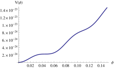
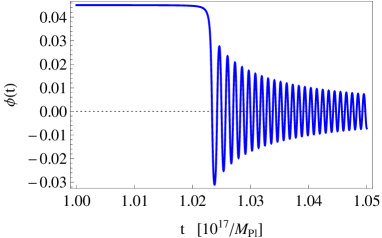
Figure 1: In the left panel, the inflaton potential is drawn by setting the parameters as $A_{1}/A_{2}=22.474579785926$ and $A_{2}=6.47\times 10^{-25}$, whereas the right panel shows the trajectory of the inflaton as a function of cosmic time $t$ for the initial value of the inflaton, $\phi_{\rm ini}=0.04508690783$.

$N$	$n_{s}$	$r$	$m_{\phi}^{2}$	$H_{\rm inf}$	$V_{\rm inf}^{1/4}$	$\frac{dn_{s}}{d\ln k}$
60.0	$0.9665$	$6.85\times 10^{-17}$	$7.92\times 10^{-21}$	$8.62\times 10^{-13}$	$1.22\times 10^{-6}$	$-2.52\times 10^{-3}$
50.0	$0.9665$	$1.61\times 10^{-16}$	$1.86\times 10^{-20}$	$1.32\times 10^{-12}$	$1.51\times 10^{-6}$	$-1.65\times 10^{-3}$

Table 1: The cosmological observables such as spectral index $n_{s}$, its running $dn_{s}/d\ln k$, tensor-to-scalar ratio $r$, Hubble scale $H_{\rm inf}$, scalar potential $V_{\rm inf}^{1/4}$ at the pivot scale and the inflaton mass $m_{\phi}^{2}$ at the vacuum. The parameters are set as $A_{1}/A_{2}=22.474579785926$ and $A_{2}=6.47\times 10^{-25}$ for the e-folding number $N=60$, whereas those are set as $A_{1}/A_{2}=22.474579787160$ and $A_{2}=6.47\times 10^{-25}$ for the e-folding number $N=50$. The initial value of the inflaton field is also set as $\phi_{{\rm ini}}=0.04508690783$ in both cases.

Tab. 1 also shows numerical results of the running, $dn_{s}/d\ln k$, which are large and negative as in the case of Ref. [21]. These values can be estimated roughly as follows. The slow-roll parameter, $\xi$, can be written

$$\xi=\frac{V_{\phi}V_{\phi\phi\phi}}{V^{2}}=\left(\frac{r}{8}\right)^{1/2}\frac{V_{\phi\phi\phi}}{V}.$$ (18)

Then, using Eq. (10) and

$$\frac{V_{\phi\phi\phi}}{V}\sim\left(\frac{\sum_{m}\frac{1}{f_{m}^{2}}}{\sum_{n}f_{n}}\right),$$ (19)

we can estimate $\xi={\cal O}(10^{-3})$ for $\eta\sim 0.01$, and this value of $\xi$ is independent of decay constants. In this model, the running is obtained as $dn_{s}/d\ln k\approx-2\xi$ and other terms are sub-dominant. Thus, it is found that $dn_{s}/d\ln k={\cal O}(10^{-3})$. Similarly, the running of running is obtained as $d^{2}n_{s}/d\ln k^{2}\approx 2\eta\xi$ in this model and other terms are sub-dominant. Then, we find that $d^{2}n_{s}/d\ln k^{2}={\cal O}(10^{-5})$, which is also independent of decay constants.

Similarly, the potential (16) with other values of $f_{1}$ and $f_{2}$ leads to results consistent with Eq. (15).

2.2 Axion monodromy inflation with sinusoidal functions

We next discuss the axion monodromy inflation with sinusoidal functions in which the general form of the axion potential is yielded by

$$V(\phi) =A_{1}\phi^{p}+\sum^{M}_{i=2}A_{i}\cos\left(\frac{\phi}{f_{i}}+\theta_{i}\right)+V_{0}.$$ (20)

Here, $\phi$ is a canonically normalized axion with the decay constants $f_{i}$; $\theta_{i}$ denotes the phase of the sinusoidal functions; $A_{i}$ are the real positive constants; and $V_{0}$ is the real constant to achieve the tiny cosmological constant. $p$ can be taken as fractional numbers or positive integers such as $p=1$ [22], $p=2/3$ [14], $p=2$ [23, 24], and $p=4/3,3$ [25], and $M$ depends on the number of hidden gauge sectors which non-perturbatively generate the potential of the axion inflaton.

We proceed to demonstrate the small-field axion inflation by the small axion decay constants $f_{i}$ in the same way as in the previous section. To obtain the sufficiently large number of e-folding, the first derivative of potential in Eq.(20),

$$V_{\phi}=A_{1}p\phi^{p-1}-\sum_{i}\frac{A_{i}}{f_{i}}\sin\left(\frac{\phi}{f_{i}}+\theta_{i}\right),$$ (21)

is required to be smaller than the potential energy, that is, $|V_{\phi}|\ll|V|$. It can be realized with the region satisfying

$$\phi\sim{\cal O}(1),$$

$$\sin(\phi/f_{i}+\theta_{i})\sim\cos(\phi/f_{i}+\theta_{i})\sim{\cal O}(1),$$ (22)

with proper signs of $\sin(\phi/f_{i}+\theta_{i})$ and $\cos(\phi/f_{i}+\theta_{i})$, and the correlated parameters in the scalar potential,

$$A_{1}p\sim\frac{A_{i}}{f_{i}}\sim\frac{A_{j}}{f_{j}},$$ (23)

for any $i,j=2,3,\cdots,M$.

Since the slow-roll inflation is realized under $|V_{\phi}|\simeq 0$ and $|V_{\phi\phi}|\simeq 0$ during the inflation, the second derivative of the potential can be estimated by employing the inflaton variation $\Delta\phi$,

$$V_{\phi\phi}\sim V_{\phi\phi\phi}\Delta\phi\sim\left(-\sum_{i}\frac{A_{i}}{f_{i}^{3}}\sin\left(\frac{\phi}{f_{i}}+\theta_{i}\right)\right)\Delta\phi,$$ (24)

for small $f_{i}$. Here, we assume that all $f_{i}^{-3}$ in the third derivative $V_{\phi\phi\phi}$ dominate the second derivative $V_{\phi\phi}$. With the help of Eqs. (22) and (23), the slow-roll parameter $\eta$ is obtained as

$$\eta\sim\frac{\sum_{i}\frac{A_{i}}{f_{i}^{3}}}{A_{1}}\Delta\phi\sim p\left(\sum_{i}\frac{1}{f_{i}^{2}}\right)\Delta\phi,$$ (25)

where the scalar potential during the inflation is approximately given by $V_{\rm inf}\sim A_{1}$ due to the conditions (22) and (23). Since we concentrate on the parameter space leading to the small-field inflation, the slow-roll parameter $\epsilon$ is expected to be much smaller than unity. It is confirmed later by checking the value of the tensor-to-scalar ratio $r=16\epsilon$. Thus, the slow-roll parameter $|\eta|$ is chosen as $10^{-2}$ to reproduce the observed spectral index $n_{s}\simeq 0.96$ reported by Planck.

By fixing $|\eta|\simeq 10^{-2}$, the tensor-to-scalar ratio is estimated by using the Lyth bound Eq.(1),

$$r\sim 10^{-2}\times(\Delta\phi)^{2}\sim 10^{-6}\times\frac{1}{p^{2}}\left(\sum_{i}\frac{1}{f_{i}^{2}}\right)^{-2}\times\left(\frac{\eta}{0.01}\right)^{2},$$ (26)

from which the power of decay constants $f$ in $r$ becomes small in comparison with that in the multi-natural inflation.

Furthermore, we can estimate the energy scale of scalar potential during the inflation $V_{\rm\inf}$ as functions of axion decay constants from Eqs. (3) and (26),

$$V_{\rm\inf}^{1/4}\sim 4\times 10^{-4}\times p^{-1/2}\left(\sum_{i}\frac{1}{f_{i}^{2}}\right)^{-1/2},$$ (27)

and consequently the Hubble parameter $H_{\rm inf}=(V_{\rm inf}/3)^{1/2}$ becomes

$$H_{\rm inf}\sim 10^{-7}\times p^{-1}\left(\sum_{i}\frac{1}{f_{i}^{2}}\right)^{-1}.$$ (28)

Finally, we estimate the inflaton mass $m_{\phi}^{2}$ as a function of the decay constant. For small $f_{i}$, the dominant term of the second derivative, $V_{\phi\phi}$, at $\phi=0$ is evaluated by using Eq. (6), $V_{\phi\phi}\sim\sum_{i}\frac{A_{i}}{f_{i}^{2}}$ and hereafter the inflaton mass is estimated as

$$m_{\phi}^{2} =V_{\phi\phi}\sim\sum_{i}\frac{A_{i}}{f_{i}^{2}}\sim\frac{\sum_{i}\frac{A_{i}}{f_{i}^{2}}}{A_{1}}V_{\rm inf}\sim p\left(\sum_{i}\frac{1}{f_{i}}\right)V_{\rm inf}\sim 3\times 10^{-14}\times p^{-1}\left(\sum_{i}\frac{1}{f_{i}}\right)\left(\sum_{i}\frac{1}{f_{i}^{2}}\right)^{-2}.$$ (29)

Let us summarize the result for two nonvanishing sinusoidal functions in Eq. (20), for simplicity. For $f_{1}\sim f_{2}\sim f\ll 1$, the obtained physical quantities have the following decay constant dependence:

$$r\sim 10^{-6}\times p^{-2}\times f^{4}\ ,\ \ \ \ V_{\rm\inf}^{1/4}\sim 4\times 10^{-4}\times p^{-1/2}\times f,$$

$$H_{\rm inf}\sim 10^{-7}\times p^{-1}\times f^{2}\ ,\ \ \ \ \ m_{\phi}^{2}\sim 3\times 10^{-14}\times p^{-1}\times f^{3}.$$ (30)

Following this line of thought, we show the numerical analysis for specific axion potentials. For the illustrative purposes, we consider the axion potential with single sinusoidal function,

$$V(\phi) = A_{1}\phi^{p}+A_{2}\left(1-\cos\left(\frac{\phi}{f}\right)\right),$$ (31)

with $f=f_{2}$, $\theta_{2}=-\pi$ and $V_{0}\simeq A_{2}$ in Eq. (20), and demonstrate the small-field axion inflation for the case with $p=2$ and small axion decay constants $f=0.1$. Fig. 2 shows the inflaton potential and the trajectory of the inflaton as a function of cosmic time $t$, where the parameters are set as $A_{1}/A_{2}=10.86169045$ and $A_{2}=6.30\times 10^{-19}$. By solving the equation of motion for the inflaton field, we numerically obtain the cosmological observables as shown in Tab. 2. It is then found that the analytical forms of physical quantities derived in Eqs. (26)-(29),

$$r \sim 10^{-6}\times\frac{1}{p^{2}}\times f^{4}\sim 3\times 10^{-11},$$

$$V_{\rm\inf}^{1/4} \sim 4\times 10^{-4}\times\frac{1}{\sqrt{p}}\times f\sim 3\times 10^{-5},$$

$$H_{\rm inf} \sim 10^{-7}\times\frac{1}{p}\times f^{2}\sim 5\times 10^{-10},$$

$$m_{\phi}^{2} \sim 3\times 10^{-14}\times\frac{1}{p}\times f^{3}\sim 8\times 10^{-17},$$ (32)

are consistent with our obtained numerical results in Tab. 2.

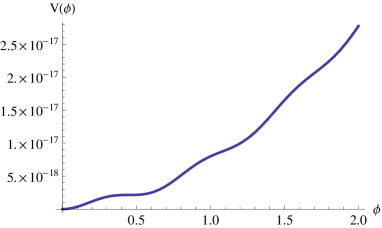
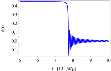
Figure 2: In the left panel, the inflaton potential is drawn by setting the parameters as $A_{1}/A_{2}=10.86169045$ and $A_{2}=6.30\times 10^{-19}$, whereas the right panel shows the trajectory of the inflaton as a function of cosmic time $t$ for the initial value of the inflaton, $\phi(0)=0.4492824$ at $t=0$.

$N$	$n_{s}$	$r$	$m_{\phi}^{2}$	$H_{\rm inf}$	$V_{\rm inf}^{1/4}$	$\frac{dn_{s}}{d\ln k}$
60.0	$0.9665$	$6.60\times 10^{-11}$	$7.67\times 10^{-17}$	$8.46\times 10^{-10}$	$3.83\times 10^{-5}$	$-2.52\times 10^{-3}$
50.0	$0.9665$	$1.55\times 10^{-10}$	$1.81\times 10^{-16}$	1.30$\times 10^{-9}$	$4.74\times 10^{-5}$	$-1.64\times 10^{-3}$

Table 2: The cosmological observables such as spectral index $n_{s}$, its running $dn_{s}/d\ln k$, tensor-to-scalar ratio $r$, Hubble scale $H_{\rm inf}$, scalar potential $V_{\rm inf}^{1/4}$ at the pivot scale and the inflaton mass $m_{\phi}^{2}$ at the vacuum. The parameters are set as $A_{1}/A_{2}=10.86169045$ and $A_{2}=6.30\times 10^{-19}$ for the e-folding number $N=60$, whereas those are set as $A_{1}/A_{2}=10.86169628$ and $A_{2}=6.30\times 10^{-19}$ for the e-folding number $N=50$. The initial value of inflaton field is also set as $\phi_{{\rm ini}}=0.4492824$ in both cases.

Tab. 2 also shows numerical results of the running, $dn_{s}/d\ln k$, and these values are large and negative, again. This value can be estimated in a way similar to the discussion in the previous section. In this model, we can estimate $\xi={\cal O}(10^{-3})$ again, which is independent of decay constants. Thus, it is found that $dn_{s}/d\ln k={\cal O}(10^{-3})$ and $d^{2}n_{s}/d\ln k^{2}={\cal O}(10^{-5})$.

Similarly, the potential (31) with other values of $p$ and $f$ leads to results consistent with Eq. (30).

3 Reheating temperature and dark matter abundance

In this section, we discuss the reheating process after the inflation dynamics. From now on, we assume that the inflaton axion discussed in the previous section couples to the gauge bosons in the standard model through tree or one-loop corrected gauge kinetic functions. In type IIB superstring theory on a toroidal background, it is known that the Kähler axion corresponding to the Kalb-Ramond field couples to the gauge boson at the tree-level, whereas the axion associated with the complex structure modulus appears in the gauge kinetic function at the one-loop level [26, 27]. In both cases, the inflaton decays into the gauge bosons $g^{(a)}$ with $a=1,2,3$ corresponding to the gauge groups of the standard model, $U(1)_{Y},SU(2)_{L},SU(3)_{C}$, and its decay width is estimated in the instantaneous decay approximation,

$$\Gamma_{\phi} = \sum_{a=1}^{3}\Gamma(\phi\rightarrow 2g^{(a)})$$ (33)

$$\simeq 5.8\times 10^{-5}c^{2}\left(\frac{m_{\phi}}{10^{13}\ {\rm GeV}}\right)^{3}\ {\rm GeV},$$

where $c$ becomes $16\pi^{2}$ and unity for the Kähler moduli and complex structure moduli. When such a decay into the gauge bosons is the dominant process, the reheating temperature is yielded as

$$T_{\rm ref}=\left(\frac{\pi^{2}g_{\ast}}{90}\right)^{-1/4}\sqrt{\Gamma_{\phi}M_{\rm Pl}}\simeq 6.4\times 10^{6}c\left(\frac{m_{\phi}}{10^{13}\ {\rm GeV}}\right)^{3/2}\ {\rm GeV},$$ (34)

with the effective degrees of freedom $g_{\ast}=106.75$.

From the results in Sec. 2.1, the reheating temperate is yielded by the axion decay constants,

$$T_{\rm ref} \simeq 5.4\times 10^{4}c\left(\frac{\sum_{m=1}^{M}\frac{1}{f_{m}}}{\sum_{n=1}^{M}f_{n}}\right)^{3/4}\left(\frac{\sum_{n=1}^{M}f_{n}}{\sum_{m=1}^{M}\frac{1}{f_{m}^{2}}}\right)^{3/2}\ {\rm GeV},$$ (35)

which is illustrated in Fig. 3 as functions of two axion decay constants for the simplified multi-natural inflation in Eq. (16). We now take into account the constraint from the isocurvature perturbation originating from the QCD axion by Eq. (2) with $f_{\rm QCD}=10^{12}\,{\rm GeV}$ and Eq. (12) with $m=1,2$, which corresponds to the blue shaded region in Fig. 3. Here and in the following analysis, we employ the maximal value of the QCD axion decay constant constrained by the upper bound of dark matter abundance, although it depends on the initial misalignment angle of the axion and dilution mechanism after the inflation [9, 10, 11]. As can be seen in Fig. 3, the smallest axion decay constant is bounded as $2\times 10^{15}\,{\rm GeV}\lesssim f\lesssim 10^{17}\,{\rm GeV}$ for the Kähler axion and $10^{16}\,{\rm GeV}\lesssim f\lesssim 10^{17}\,{\rm GeV}$ for the axion of complex structure modulus, where the lower bounds are put by $T_{\rm reh}\gtrsim{\cal O}(5)$ MeV in order not to spoil the successful BBN, whereas the upper bounds are set by the constraint from the isocurvature perturbation of the QCD axion with $f_{\rm QCD}=10^{12}\,{\rm GeV}$.

Figure 3: The reheating temperature $T_{\rm reh}$ as functions of two decay constants $f_{1,2}$ for the case of the axion of Kähler moduli in the left panel and that of the complex structure modulus in the right panel. In both panels, the solid, dashed, dotdashed and dotted curves represent the reheating temperatures, $T_{\rm reh}=1,10,10^{2},10^{3}\,{\rm MeV}$, respectively. The blue shaded region is excluded by the isocurvature perturbation originating from the QCD axion.

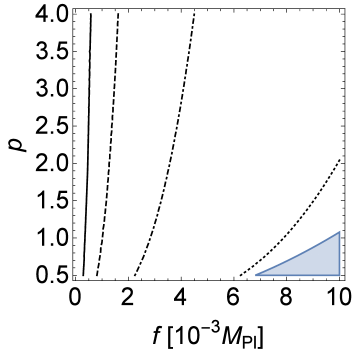
Figure 4: The reheating temperature $T_{\rm reh}$ as functions of decay constant $f$ and the power of he polynomial term $p$ for the case of the axion of Kähler moduli in the left panel and that of the complex structure modulus in the right panel. In both panels, the solid, dashed and dotdashed curves represent the reheating temperatures, $T_{\rm reh}=1,10,10^{2},10^{3}\,{\rm MeV}$, respectively. The blue shaded region is excluded by the isocurvature perturbation originating from the QCD axion.

Similarly, the reheating temperate for the axion monodromy inflation with sinusoidal functions in Sec. 2.2 is also dominated by the axion decay constants,

$$T_{\rm ref} \simeq 5.4\times 10^{4}c\ p^{-3/4}\left(\sum_{i=2}^{M}\frac{1}{f_{i}}\right)^{3/4}\left(\sum_{i=2}^{M}\frac{1}{f_{i}^{2}}\right)^{-3/2}\ {\rm GeV},$$ (36)

which is illustrated in Fig. 4 as functions of the axion decay constant $f=f_{2}\,(M=2)$ and the power of polynomial $p$ for the simplified axion monodromy inflation with sinusoidal functions in Eq. (31). In Fig. 4 and in what follows, $p$ is considered the continuous parameter for simplicity, although it is a fractional number derived in a detailed string setup. In a similar fashion as in the multi-natural inflation, the blue shaded region in Fig. 4 is excluded by the isocurvature perturbation originating from the QCD axion which is estimated by employing Eq. (2) with $f_{\rm QCD}=10^{12}\,{\rm GeV}$ and Eq. (28) with $f=f_{2}$. In order not to spoil the successful BBN and overproduce the isocurvature perturbation due to the QCD axion, Fig. 4 gives the bounds $2\times 10^{14}\,{\rm GeV}\lesssim f\lesssim 5\times 10^{16}\,{\rm GeV}$ for the Kähler axion and $2\times 10^{15}\,{\rm GeV}\lesssim f\lesssim 5\times 10^{16}\,{\rm GeV}$ for the axion of the complex structure modulus. Note that the smaller $f_{\rm QCD}$ gives the tight upper bound on $f$ from the isocurvature perturbation of the QCD axion. As a result, these regions correspond to the typical decay constant for the closed string axions [2, 3, 4]. That is surprisingly interesting. Although we focus on the simplified axion potentials in Eqs. (16) and (31), such severe constraints for the axion decay constant are also applied to the general form of the axion potential. Indeed, the larger axion decay constants lead to the large Hubble scale given in Eqs. (12) and (28).

From these considerations, the low-scale axion decay constants realizing the successful small-field axion inflations generically predict the low reheating temperature. It implies that the freeze-out temperature of dark matter would be smaller than the reheating temperature and consequently the dark matter yield is determined by the non-thermal process from the inflaton decay

$$\frac{n_{\rm dm}}{s}\simeq\frac{3T_{\rm reh}}{4m_{\phi}}{\rm Br}_{\rm dm}\simeq 4.8\times 10^{-7}c\,{\rm Br}_{\rm dm}\left(\frac{m_{\phi}}{10^{13}\ {\rm GeV}}\right)^{1/2},$$ (37)

where $n_{\rm dm}$ is the number density of dark matter, $s$ is the entropy density of the Universe and ${\rm Br}_{\rm dm}$ is the branching ratio from the inflaton to dark matter. The relic abundance of dark mater is then given in terms of the ratio of the critical density to the current entropy density of the Universe $\rho_{\rm cr}/s_{0}\simeq 3.6h^{2}\times 10^{-9}$,

$$\Omega_{\rm dm}h^{2}\simeq m_{\rm dm}\frac{n_{\rm dm}}{s}\frac{s_{0}}{\rho_{\rm cr}}\simeq 1.3c\left(\frac{m_{\rm dm}}{100\,{\rm GeV}}\right)\left(\frac{{\rm Br}_{\rm dm}}{10^{-4}}\right)\left(\frac{m_{\phi}}{10^{13}\ {\rm GeV}}\right)^{1/2},$$ (38)

with $h$ being the dimensionless Hubble parameter.

From now on, we for simplicity assume that the current dark matter abundance mainly consists of the QCD axion compared with another cold dark matter. In Figs. 5 and 6, we plot the dark matter abundance for the simplified multi-natural inflation in Eq. (16),

$$\Omega_{\rm dm}h^{2}\simeq 0.27c\left(\frac{m_{\rm dm}}{100\,{\rm GeV}}\right)\left(\frac{{\rm Br}_{\rm dm}}{10^{-4}}\right)\left(\frac{\sum_{m=1}^{2}\frac{1}{f_{m}}}{\sum_{n=1}^{2}f_{n}}\right)^{1/4}\left(\frac{\sum_{n=1}^{2}f_{n}}{\sum_{m=1}^{2}\frac{1}{f_{m}^{2}}}\right)^{1/2},$$ (39)

and for the simplified axion monodromy inflation with sinusoidal functions in Eq. (31),

$$\Omega_{\rm dm}h^{2}\simeq 0.27c\left(\frac{m_{\rm dm}}{100\,{\rm GeV}}\right)\left(\frac{{\rm Br}_{\rm dm}}{10^{-4}}\right)2^{-1/4}f^{3/4},$$ (40)

respectively. The relic dark matter abundance should be less than $\Omega_{\rm dm}h^{2}\simeq 0.12$ reported by Planck in order to not overclose our Universe [7]. Although these predictions depend on the branching ratio ${\rm Br}_{\rm dm}$ and dark matter mass, $\Omega_{\rm dm}h^{2}<0.12$ in Figs. 5 and 6 is achieved in both inflation models. For example, in simplified multi-natural inflation in Eq. (16), $\Omega_{\rm dm}h^{2}<0.12$ can be realized under e.g., ${\rm Br}_{\rm dm}<{\cal O}(10^{-4})$ and $m_{\rm dm}\simeq 100\,{\rm GeV}$ with $f_{1,2}\simeq 2\times 10^{-3}\,{\rm M_{\rm Pl}}$ for the Kähler axion and ${\rm Br}_{\rm dm}<{\cal O}(10^{-3})$ and $m_{\rm dm}\simeq 100\,{\rm GeV}$ with $f_{1,2}\simeq 2\times 10^{-2}\,{\rm M_{\rm Pl}}$ for the axion of the complex structure modulus, whereas in axion monodromy inflation with sinusoidal functions in Eq. (31), $\Omega_{\rm dm}h^{2}<0.12$ can be realized under e.g., ${\rm Br}_{\rm dm}<{\cal O}(10^{-4})$ and $m_{\rm dm}\simeq 100\,{\rm GeV}$ with $f\simeq 3\times 10^{-4}\,{\rm M_{\rm Pl}}$ for the Kähler axion and ${\rm Br}_{\rm dm}<{\cal O}(10^{-3})$ and $m_{\rm dm}\simeq 100\,{\rm GeV}$ with $f\simeq 10^{-2}\,{\rm M_{\rm Pl}}$ for the axion of complex structure modulus. However, the low-scale inflation requires enough baryon asymmetry to reproduce the current baryon asymmetry of our Universe. To explain the relic baryon asymmetry, we could combine our inflation models with the baryogenesis scenario, e.g., the Affleck-Dine mechanism [28, 29]. It would be studied in a future work.

Figure 5: The dark matter abundance $\Omega_{\rm dm}h^{2}=0.1$ as functions of two decay constants $f_{1,2}$ for the case of the axion of the Kähler moduli in the left panel and that of the complex structure modulus in the right panel. In the left panel, the black solid, dashed, and dotdashed curves are drawn by setting $m_{\rm dm}{\rm Br}_{\rm dm}=10^{-2},0.02,0.05\,{\rm GeV}$, respectively, whereas, in the right panel, the black solid, dashed and dotdashed curves are drawn by setting $m_{\rm dm}{\rm Br}_{\rm dm}=10^{-1},0.2,1\,{\rm GeV}$, respectively. The blue shaded region is excluded by the isocurvature perturbation originating from the QCD axion with $f_{\rm QCD}=10^{12}\,{\rm GeV}$.

Figure 6: The dark matter abundance $\Omega_{\rm dm}h^{2}=0.1$ as functions of decay constant $f$ and the power of polynomial term $p$ for the case of the axion of the Kähler moduli in the left panel and that of the complex structure modulus in the right panel. In the left panel, the black solid, dashed and dotdashed curves are drawn by setting $m_{\rm dm}{\rm Br}_{\rm dm}=10^{-2},0.02,0.05\,{\rm GeV}$, respectively, whereas, in the right panel, the black solid, dashed, and dotdashed curves are drawn by setting $m_{\rm dm}{\rm Br}_{\rm dm}=0.15,0.2,0.4\,{\rm GeV}$, respectively. The blue shaded region is excluded by the isocurvature perturbation originating from the QCD axion with $f_{\rm QCD}=10^{12}\,{\rm GeV}$.

4 Conclusion

We have discussed the general class of small-field axion inflation, which is the mixture of polynomial and sinusoidal functions with an emphasis on the small axion decay constant compared with the Planck scale. In contrast to the large-field axion inflation such as the natural inflation [1] and axion monodromy inflation [14], the small-field axion inflation predicts the small amount of primordial gravitational waves and low inflation scale. This class of inflation models is motivated by the weak gravity conjecture, which prohibits the trans-Planckian axion decay constant and the constraint from isocurvature perturbation due to the QCD axion. When the axion decay constants and parameters in the scalar potential satisfy the certain conditions leading to the successful small-field axion inflations as discussed in Sec. 2, we find that the cosmological observables are written in terms of the axion decay constants in a systematic way.

Furthermore, the axion decay constant is severely constrained within the range $10^{14}\,{\rm GeV}\lesssim f\lesssim 10^{17}\,{\rm GeV}$, where the lower bounds are put by $T_{\rm reh}\gtrsim{\cal O}(5)$ MeV in order not to spoil the successful BBN, whereas the upper bounds are set by the constraint from the isocurvature perturbation due to the QCD axion with $f_{\rm QCD}=10^{12}\,{\rm GeV}$. This constrained axion decay constant naturally appears in the string theory, when our discussed axion corresponds to the closed string axion [2, 3, 4]. Although the parameters in the axion potential should be properly chosen to achieve a flat enough direction in the axion potential, the small-field axion inflation is attractive from the theoretical and phenomenological points of view.

References

- [1] K. Freese, J. A. Frieman and A. V. Olinto, Phys. Rev. Lett. 65 (1990) 3233.
- [2] K. Choi and J. E. Kim, Phys. Lett. B 154 (1985) 393 Erratum: [Phys. Lett. B 156 (1985) 452].
- [3] T. Banks, M. Dine, P. J. Fox and E. Gorbatov, JCAP 0306 (2003) 001 [hep-th/0303252].
- [4] P. Svrcek and E. Witten, JHEP 0606 (2006) 051 [hep-th/0605206].
- [5] D. H. Lyth, Phys. Rev. Lett. 78 (1997) 1861 [hep-ph/9606387].
- [6] P. A. R. Ade et al. [Planck Collaboration], Astron. Astrophys. 571 (2014) A22 [arXiv:1303.5082 [astro-ph.CO]].
- [7] P. A. R. Ade et al. [Planck Collaboration], Astron. Astrophys. 594 (2016) A20 [arXiv:1502.02114 [astro-ph.CO]].
- [8] N. Arkani-Hamed, L. Motl, A. Nicolis and C. Vafa, JHEP 0706 (2007) 060 [hep-th/0601001].
- [9] M. Kawasaki and F. Takahashi, Phys. Lett. B 618 (2005) 1 [hep-ph/0410158].
- [10] H. Hattori, T. Kobayashi, N. Omoto and O. Seto, Phys. Rev. D 92 (2015) no.10, 103518 [arXiv:1510.03595 [hep-ph]].
- [11] K. Akita, T. Kobayashi, A. Oikawa and H. Otsuka, JHEP 1605 (2016) 178 [arXiv:1603.08399 [hep-ph]].
- [12] T. Kobayashi, A. Oikawa and H. Otsuka, Phys. Rev. D 93 (2016) no.8, 083508 [arXiv:1510.08768 [hep-ph]].
- [13] K. Kadota, T. Kobayashi, A. Oikawa, N. Omoto, H. Otsuka and T. H. Tatsuishi, JCAP 1610 (2016) no.10, 013 [arXiv:1606.03219 [hep-ph]].
- [14] E. Silverstein and A. Westphal, Phys. Rev. D 78 (2008) 106003 [arXiv:0803.3085 [hep-th]].
- [15] T. Kobayashi, O. Seto and Y. Yamaguchi, PTEP 2014 (2014) no.10, 103E01 [arXiv:1404.5518 [hep-ph]].
- [16] T. Higaki, T. Kobayashi, O. Seto and Y. Yamaguchi, JCAP 1410 (2014) no.10, 025 [arXiv:1405.0775 [hep-ph]].
- [17] K. Choi, H. Kim and S. Yun, Phys. Rev. D 90 (2014) 023545 [arXiv:1404.6209 [hep-th]].
- [18] M. Czerny and F. Takahashi, Phys. Lett. B 733 (2014) 241 [arXiv:1401.5212 [hep-ph]].
- [19] M. Czerny, T. Higaki and F. Takahashi, JHEP 1405 (2014) 144 [arXiv:1403.0410 [hep-ph]].
- [20] H. Abe, T. Kobayashi and H. Otsuka, JHEP 1504, 160 (2015) [arXiv:1411.4768 [hep-th]].
- [21] S. Parameswaran, G. Tasinato and I. Zavala, JCAP 1604 (2016) no.04, 008 [arXiv:1602.02812 [astro-ph.CO]].
- [22] L. McAllister, E. Silverstein and A. Westphal, Phys. Rev. D 82 (2010) 046003 [arXiv:0808.0706 [hep-th]].
- [23] E. Palti and T. Weigand, JHEP 1404 (2014) 155 [arXiv:1403.7507 [hep-th]].
- [24] N. Kaloper and L. Sorbo, Phys. Rev. Lett. 102 (2009) 121301 [arXiv:0811.1989 [hep-th]].
- [25] L. McAllister, E. Silverstein, A. Westphal and T. Wrase, JHEP 1409 (2014) 123 [arXiv:1405.3652 [hep-th]].
- [26] D. Lust and S. Stieberger, Fortsch. Phys. 55 (2007) 427 [hep-th/0302221].
- [27] R. Blumenhagen, B. Kors, D. Lust and S. Stieberger, Phys. Rept. 445 (2007) 1 [hep-th/0610327].
- [28] I. Affleck and M. Dine, Nucl. Phys. B 249 (1985) 361.
- [29] M. Dine, L. Randall and S. D. Thomas, Nucl. Phys. B 458 (1996) 291 [hep-ph/9507453].