A Database of Phase Calibration Sources and their Radio Spectra for the Giant Metrewave Radio Telescope

Abstract

We are pursuing a project to build a database of phase calibration sources suitable for Giant Metrewave Radio Telescope (GMRT). Here we present the first release of 45 low frequency calibration sources at 235 MHz and 610 MHz. These calibration sources are broadly divided into quasars, radio galaxies and unidentified sources. We provide their flux densities, models for calibration sources, ($u,v$) plots, final deconvolved restored maps and clean-component lists/files for use in the Astronomical Image Processing System (aips) and the Common Astronomy Software Applications (casa). We also assign a quality factor to each of the calibration sources. These data products are made available online through the GMRT observatory website. In addition we find that (i) these 45 low frequency calibration sources are uniformly distributed in the sky and future efforts to increase the size of the database should populate the sky further, (ii) spectra of these calibration sources are about equally divided between straight, curved and complex shapes, (iii) quasars tend to exhibit flatter radio spectra as compared to the radio galaxies or the unidentified sources, (iv) quasars are also known to be radio variable and hence possibly show complex spectra more frequently, and (v) radio galaxies tend to have steeper spectra, which are possibly due to the large redshifts of distant galaxies causing the shift of spectrum to lower frequencies.

1 Introduction

The Giant Metrewave Radio telescope (GMRT, Swarup et al., 1991) is the most sensitive radio telescope in the world that is capable of operating at low radio frequencies from 150 MHz to 1450 MHz. In order to obtain reliable information about target astronomical sources, radio sources whose structure and flux density are known a priori are routinely observed to determine antenna based calibration solutions. Any errors in the models used for these calibration sources reflect in errors in the antenna based calibration solutions, especially in the phase, and limit the quality of the radio images obtained. GMRT users have traditionally been using phase calibration sources from the Very Large Array (VLA) calibrator manual (2016), which is biased towards observations optimized for higher frequencies. In this paper we present a new database which is intended to facilitate science operations at the GMRT. The database presenting all products, i.e., their flux densities, models, ($u,v$) plots, final deconvolved restored maps and clean-component lists/files (Cornwell, Braun & Briggs, 1999; Högbom, 1974), is available at the ‘Observing Help’ web-page of the GMRT observatory.

In this paper, our motivations for such a database are discussed in Sect. 2. The sample is presented in Sect. 3 and its archival data and data reduction are detailed in Sect. 4 and Sect. 4.1, respectively. The results from the database, i.e., their quality standards, sky distribution, comparison of images made using image model from the database and made in a routine manner and radio properties are discussed in Sect. 5.1, Sect. 5.2, Sect. 5.3 and Sect. 5.4, respectively. Finally, we provide a summary in Sect. 6.

2 Motivations

The process of removing effects of phase and amplitude corruption from interferometer data is called calibration (Fomalont & Perley, 1999). Several complexities and levels in the calibration of interferometric instruments exist, for example, errors due to (i) changes in the length of transmission system or receiver sensitivity and the electronics, (ii) inaccurate antenna positions (i.e., geometric errors), which are typically known to $\approx$ cm–m, and (iii) changes in the visibility induced by the atmosphere, including ionosphere (Beasley & Conway, 1999). The observed visibility phase is defined as the relative phase of the electric fields measured simultaneously at two points along the wavefront from the radio sources. The atmospheric effects on this phase can be important on timescales ranging from less than a minute to hours or more.

Mathematically, the error in observed visibility phase $\phi_{\rm obs}(t,~{}\nu)$ from the correlator can be expressed as

$$\begin{split}\phi_{\rm obs}(t,~{}\nu)=\phi_{\rm true}(t,~{}\nu)+\phi_{\rm inst}(t,~{}\nu)\\ +\phi_{\rm geom}(t,~{}\nu)+\phi_{\rm atmos}(t,~{}\nu)\end{split}$$

where $\phi_{\rm true}(t,~{}\nu)$ is the true visibility phase, $\phi_{\rm inst}(t,~{}\nu)$ is the sum of all instrumental phase errors at the two antennas and is possibly due to propagation through the antenna optics and electronics before the sampled electric field is digitized, $\phi_{\rm geom}(t,~{}\nu)$ is the phase error due to geometrical errors in the delay model and $\phi_{\rm atmos}(t,~{}\nu)$ represent the effects of different atmospheric delays above each antenna. Note that both the ionospheric and the tropospheric (Thompson et al., 2001; Carilli & Holdaway, 1999) errors are included in phase errors due to the atmosphere. The dominant sources of errors at low frequencies ($\lesssim$ 1 GHz) are refraction, propagation delay and Faraday rotation caused by the ionosphere, while at high frequencies ($\gtrsim$ 1 GHz) they are scattering, effects of water vapor and propagation delay caused by the troposphere (Thompson et al., 2001). Instrumental, $\phi_{\rm inst}(t,~{}\nu)$ and geometrical, $\phi_{\rm geom}(t,~{}\nu)$ errors can be reduced to acceptable levels by good design, but corrections for changes in the visibility due to the atmosphere are not possible, since these changes affect visibility phases. It is well known that the ionosphere severely limits the phase stability of radio interferometers at low radio frequencies (Intema et al., 2009). In practice, if $\phi_{\rm obs}(t,~{}\nu)$ varies by a full turn over time or frequency-channel, it limits an observer’s ability to integrate data over time and frequency. Several techniques are available that use interferometry to overcome the limits imposed by the atmosphere. The technique of making observations of a bright nearby point source, called the ‘phase’ calibration source, frequently interspersed with the target source is called phase referencing (Beasley & Conway, 1999). This technique of phase referencing has been used successfully to allow correction of the fast temporal changes of relative phases of individual antennas of the interferometer.

Methodologically, consider the nodding style, where observations at time $t_{2}$ of the target source are interleaved between calibration observations at $t_{1}$ and $t_{3}$ of the phase calibration source. The observed phases for calibration source and target source, $\phi_{\rm obs}^{\rm c}$ and $\phi_{\rm obs}^{\rm t}$, respectively, will be

$$\begin{split}\phi_{\rm obs}^{\rm c}(t_{1},~{}\nu)=\phi_{\rm true}^{\rm c}(t_{1},~{}\nu),~{}\nu+\phi_{\rm inst}^{c}(t_{1},~{}\nu)\\ +\phi_{\rm geom}^{c}(t_{1},~{}\nu)+\phi_{\rm atmos}^{c}(t_{1},~{}\nu),\end{split}$$

$$\begin{split}\phi_{\rm obs}^{\rm t}(t_{2},~{}\nu)=\phi_{\rm true}^{\rm t}(t_{2},~{}\nu)+\phi_{\rm inst}^{t}(t_{2},~{}\nu)\\ +\phi_{\rm geom}^{t}(t_{2},~{}\nu)+\phi_{\rm atmos}^{t}(t_{2},~{}\nu),\end{split}$$

$$\begin{split}\phi_{\rm obs}^{\rm c}(t_{3},~{}\nu)=\phi_{\rm true}^{\rm c}(t_{3},~{}\nu)+\phi_{\rm inst}^{c}(t_{3},~{}\nu)\\ +\phi_{\rm geom}^{c}(t_{3},~{}\nu)+\phi_{\rm atmos}^{c}(t_{3},~{}\nu).\end{split}$$

Next let us represent the interpolated phase of calibration source at time $t_{2}$, by

$$\begin{split}\phi_{\rm obs}^{\prime~{}{\rm c}}(t_{2},~{}\nu)=\phi_{\rm true}^{\prime~{}{\rm c}}(t_{2},~{}\nu)+\phi_{\rm inst}^{\prime~{}{\rm c}}(t_{2},~{}\nu)\\ +\phi_{\rm geom}^{\prime~{}{\rm c}}(t_{2},~{}\nu)+\phi_{\rm atmos}^{\prime~{}{\rm c}}(t_{2},~{}\nu)\end{split}$$

where the interpolated quantities are indicated by primes. The difference between the phases of the target source and the interpolated calibration source will be

$$\begin{split}\phi_{\rm obs}^{\rm t}-\phi_{\rm obs}^{\prime~{}{\rm c}}=(\phi_{\rm true}^{\rm t}-\phi_{\rm true}^{\prime~{}{\rm c}})+(\phi_{\rm inst}^{\rm t}-\phi_{\rm inst}^{\prime~{}{\rm c}})\\ +(\phi_{\rm geom}^{t}-\phi_{\rm geom}^{\prime~{}{\rm c}})+(\phi_{\rm atmos}^{t}-\phi_{\rm atmos}^{\prime~{}{\rm c}}).\end{split}$$

Here, we have ignored the $t_{2}$ and $\nu$ notations. Also, we have determined the telescope phase corrections using the calibration source and applied to the target source using a suitable interpolation function. Now we make three reasonable assumptions: (i) The target source and the calibration source are located roughly in the same region of the sky, or in other words corrections for one source also apply to the other, so that

$$\phi_{\rm atmos}^{t}-\phi_{\rm atmos}^{\prime~{}{\rm c}}=0.$$

This is called the ‘isoplanarity’ assumption. (ii) If there exist instrumental errors, they would be the same for the target source and the phase calibration source due to the design of the instrument,

$$\phi_{\rm inst}^{\rm t}-\phi_{\rm inst}^{\prime~{}{\rm c}}=0,$$

and (iii) if there exist geometrical errors, e.g., antenna position errors, they, too will be the same for two sources with a small separation between target source and calibration source,

$$\phi_{\rm geom}^{t}-\phi_{\rm geom}^{\prime~{}{\rm c}}=0.$$

Thus we obtain,

$$\phi_{\rm obs}^{\rm t}-\phi_{\rm obs}^{\prime~{}{\rm c}}=(\phi_{\rm true}^{\rm t}-\phi_{\rm true}^{\prime~{}{\rm c}}).$$

Furthermore, either the calibration source is bright, point-like and the only source in the field-of-view or we a priori know the model of the field-of-view containing the calibration source, then we can assume

$$\phi_{\rm true}^{\prime~{}{\rm c}}=0.$$

The phase-referenced difference phase then contains only information about the target source structure, and the positions of the target source and calibration source. Fourier inverting and deconvolving the ‘phase-calibrated’ target source data should provide us with a good image of the target source.

3 Sample

The VLA varies its angular resolution through movement of its antennas, and hence has four basic antenna configurations, A, B, C and D, whose scales vary by the ratios 35.5:10.8:3.28:1 (VLA observational status summary, 2017). GMRT, unlike the VLA, has a hybrid configuration, with 14 antennas in a central array and the remaining 16 antennas spread across three arms of a ‘Y’ (Swarup et al., 1991). The central array yields baselines of $\lesssim$ 1 km and the longer baselines of the ‘Y’ yield baselines up to a maximum length of $\sim$ 25 km, i.e., ($u,v$) coverages out to $\sim$ 0.8 k$\lambda$ and $\sim$ 20 k$\lambda$, respectively at 235 MHz. In other words, a single observation with the GMRT yields information from small to large angular scales, which in the case of the VLA must be provided by using several of its antenna configurations. The quality of VLA calibration sources varies with frequency and configuration (VLA observational status summary, 2017). Their absolute position errors range from $<$0.002 arcsec (code ‘A’, VLA observational status summary, 2017) to $>$0.15 arcsec (code ‘T’, VLA observational status summary, 2017). Correspondingly the phase calibration errors have several levels, from as small as $<$3% errors (P-class) or 10% errors (S-class) to confused or to unknown or inappropriate. We selected a list of target calibration sources from the VLA calibrator manual (2016) which met the following criteria: The source should be bright, i.e., have flux density at 20 cm, S${}_{\rm 20~{}cm}$ $>$ 0.5 Jy and (i) should be P-class at A-array and B-array VLA configurations, and (ii) either P-class or S-class at C-array and D-array VLA configurations. These criteria provided us with 121 sources, whose positional uncertainties in right ascension and declination are $<$ 0.15 arcsec (VLA observational status summary, 2017). We used this list of 121 phase calibration sources to look for archival GMRT data and found observations for 45 (34%) sources listed in Table 1 at 235 MHz and 610 MHz. New observations were made only for a handful of sources when the archival data were badly affected by radio frequency interference (RFI) or challenging ionospheric conditions; otherwise no new GMRT observations were made for this project.

These phase calibration sources are broadly divided among three categories, (i) quasars, (ii) giga-hertz peaked sources, compact steep-spectrum sources and radio galaxies, which we refer indiscriminately as radio galaxies in what follows, and (iii) unidentified sources (see also Table 1). Below we present data and its analysis (Sect. 4 and 4.1) of first release of these 45 sources, forming our database of phase calibration sources.

4 Archival Data

Table 1: The observing log for phase calibration sources. The columns are as follows: (1) calibration source name. which encodes the J2000 position; (2) observing date; and (3) flux density and bandpass calibrator. Columns (4), (5) and (6), and (7), (8) and (9), respectively are for 235 MHz and 610 MHz data, where these columns are as follows: (4, 7) nominal and effective bandwidth; (5, 8) integration time; and (6, 9) FWHM of the elliptical Gaussian restoring beam and position angle (P.A.).

			235 MHz				610 MHz
Calibrator	Obs-date Flux density		$\Delta\nu$     tint		Synthesized, P.A.		$\Delta\nu$     tint		Synthesized, P.A.
(J2000)	calibrator				beam				beam
			(MHz)   (min)		(arcsec2, deg)		(MHz)   (min)		(arcsec2, deg)
(1)	(2)	(3)	(4)       (5)		(6)		(7)       (8)		(9)
Radio galaxies
0010$-$418	2013-07-05	3C48	16 / 15.2	67	21.5 $\times$ 10.3, 21.6		32 / 31.2	85	14.3 $\times$ 6.5, 14.8
0029$+$349	2006-07-10	3C48	16 / 14.9	33	13.2 $\times$ 9.9, 41.9		32 / 30.8	33	5.4 $\times$ 4.1, 50.3
0119$+$321	2007-08-17	3C48	6 / 5.4	58	14.1 $\times$ 9.7, 71.7		32 / 30.8	58	6.0 $\times$ 4.7, 82.5
0410$+$769	2005-01-22	3C147	6 / 4.9	167	18.0 $\times$ 14.6, $-$86.3		16 / 15.0	173	10.8 $\times$ 5.8, $-$68.8
0745$+$101	2011-11-17	3C48					16 / 15.2	89	7.1 $\times$ 6.1, 37.2
0943$-$083	2008-12-05	3C48					16 / 15.2	71	5.3 $\times$ 4.8, 27.8
1130$-$148	2009-06-06	3C286	6 / 5.2	53	16.3 $\times$ 10.8, 21.3		32 / 31.4	53	7.1 $\times$ 4.6, 21.2
1313$+$675	2011-02-12	3C147	6 / 4.9	48	16.9 $\times$ 13.1, $-$53.2		32 / 31.0	48	6.5 $\times$ 5.4, $-$51.8
1400$+$621	2004-01-02	3C48					16 / 14.6	62	9.3 $\times$ 5.0, $-$45.6
1445$+$099	2008-07-22	3C147	6 / 5.1	52	12.0 $\times$ 10.1, 84.1		32 / 31.2	62	5.2 $\times$ 4.2, 59.6
1602$+$334	2009-06-06	3C286	6 / 5.1	51	12.6 $\times$ 10.1, 5.8		32 / 31.4	51	5.7 $\times$ 5.0, 9.4
1944$+$548	2013-07-12	3C48	16 / 15.3	57	14.8 $\times$ 11.8, $-$50.8		32 / 31.0	57	6.1 $\times$ 5.1, $-$49.0
2011$-$067	2008-12-06	3C286	6 / 4.9	25	14.6 $\times$ 9.6, 48.0		32 / 31.2	65	5.6 $\times$ 4.6, 48.1
2212$+$018	2008-08-10	3C147	6 / 5.3	34	14.8 $\times$ 11.0, 32.0		32 / 31.2	34	6.2 $\times$ 5.3, $-$1.3
2344$+$824	2013-07-24	3C48	16 / 15.1	49	23.5 $\times$ 9.4, $-$54.1		32 / 31.0	49	12.2 $\times$ 5.3, $-$62.4
2355$+$498	2013-07-24	3C48	16 / 15.1	24	15.0 $\times$ 9.5, $-$52.1		32 / 31.0	50	8.5 $\times$ 4.7, $-$74.1
Quasars
0024$-$420	2013-07-05	3C48	16 / 15.2	67	21.5 $\times$ 10.3, 21.6		32 / 31.2	84	10.8 $\times$ 6.6, 18.8
0059$+$001	2006-07-22	3C48	6 / 5.2	36	13.4 $\times$ 10.3, 57.3		32 / 31.3	67	6.3 $\times$ 4.7, 62.7
0102$+$584	2013-07-12	3C48	16 / 15.3	55	12.1 $\times$ 9.6, $-$6.9		32 / 31.3	57	5.9 $\times$ 4.6, 6.6
0136$+$478	2013-07-12	3C48	16 / 15.3	37	12.0 $\times$ 9.7, 29.2		32 / 31.0	57	5.3 $\times$ 4.2, 27.2
0217$+$738	2013-07-12	3C48	16 / 15.3	10	18.6 $\times$ 9.0, 1.8		32 / 31.0	58	7.7 $\times$ 4.5, 11.9
0238$+$166	2007-08-17	3C48	6 / 5.4	45	14.8 $\times$ 11.3, $-$89.5		32 / 30.8	45	7.4 $\times$ 4.7, 85.6
0240$-$231	2008-07-21	3C147	6 / 5.1	63	15.6 $\times$ 12.1, $-$17.7		32 / 31.2	63	6.9 $\times$ 5.2, $-$13.0
0303$+$472	2009-10-25	3C48	6 / 5.0	99	13.5 $\times$ 10.8, 66.9		32 / 31.4	99	6.2 $\times$ 5.3, $-$77.4
0414$+$343	2013-07-26	3C48	16 / 15.1	57	11.2 $\times$ 7.9, 54.3		32 / 31.0	57	5.5 $\times$ 4.5, 73.1
0555$+$398	2009-11-20	3C147					16 / 15.2	57	6.3 $\times$ 4.2, 75.2
0607$-$085	2008-08-10	3C147	6 / 5.3	25	15.2 $\times$ 11.2, 14.1		32 / 31.2	22	7.0 $\times$ 5.1, $-$8.0
0739$+$016	2008-07-21	3C147	6 / 5.1	61	13.8 $\times$ 11.4, $-$75.4		32 / 31.2	61	6.3 $\times$ 4.8, $-$60.0
1150$-$003	2008-07-22	3C48	6 / 5.1	67	13.2 $\times$ 12.2, 71.1		32 / 31.2	67	5.7 $\times$ 4.7, 59.1
1254$+$116	2008-07-21	3C147	6 / 5.1	54	13.0 $\times$ 10.5, 63.1		32 / 31.2	54	5.1 $\times$ 3.6, 63.9
1613$+$342	2002-12-21	3C286	6 / 4.9	48	17.4 $\times$ 10.6, $-$79.7		6 / 5.4	48	5.2 $\times$ 4.9, 68.9
1743$-$038	2006-07-20	3C286	6 / 5.2	55	13.8 $\times$ 11.8, 56.6		32 / 31.3	54	6.8 $\times$ 4.9, 28.6
1923$-$210	2008-07-22	3C147	6 / 5.1	53	14.6 $\times$ 10.8, 23.3		32 / 31.2	53	6.4 $\times$ 4.3, 26.7
2005$+$778	2013-07-12	3C48	16 / 15.3	56	22.1 $\times$ 11.9, $-$37.7		32 / 31.0	57	8.6 $\times$ 4.6, $-$34.3
2015$+$371	2013-08-13	3C48	16 / 15.0	57	19.7 $\times$ 12.3, 84.1		32 / 31.0	57	8.1 $\times$ 5.0, 82.3
2025$+$337	2013-08-13	3C48	16 / 15.0	55	20.8 $\times$ 12.8, 79.2		32 / 31.0	55	8.5 $\times$ 5.0, 77.8
2202$+$422	2013-08-02	3C48	16 / 15.0	48	11.3 $\times$ 10.7, 65.2		32 / 31.0	48	7.0 $\times$ 4.9, $-$69.3
2236$+$284	2008-08-10	3C147	6 / 5.3	21	14.7 $\times$ 12.2, $-$44.7		32 / 31.2	21	6.9 $\times$ 5.0, $-$48.2
2254$+$247	2013-07-24	3C48	16 / 15.1	44	16.4 $\times$ 10.2, 75.5		32 / 31.0	44	9.9 $\times$ 4.7, 87.2
Unidentified sources
0110$+$565	2003-01-13	3C147	6 / 5.3	69	14.8 $\times$ 11.0, 45.0		6 / 5.4	69	6.1 $\times$ 4.9, 54.5
0321$+$123	2004-03-27	3C286					16 / 15.2	91	7.3 $\times$ 5.0, 17.4
0438$+$488	2013-07-26	3C48	16 / 15.1	46	13.0 $\times$ 8.7, 53.5		32 / 31.0	57	6.0 $\times$ 4.6, 56.7
0632$+$103	2004-07-24	3C147	6 / 4.9	63	13.0 $\times$ 10.4, 71.6		32 / 31.0	64	7.7 $\times$ 4.1, 57.8
1513$+$236	2008-07-27	3C286	6 / 5.1	44	13.2 $\times$ 10.8, 72.0		32 / 31.2	49	5.6 $\times$ 4.5, 66.9
2023$+$544	2013-07-12	3C48	16 / 15.3	32	13.7 $\times$ 11.1, $-$23.4		32 / 31.0	56	6.0 $\times$ 5.3, $-$34.9

Typical GMRT continuum observations are bracketed and interleaved by primary (flux density and bandpass) calibration source scans on 3C 48, 3C 147 and 3C 286 of 10–20 minute duration. Interleaved in these observations are several secondary (phase) calibration source scans, each of a few minutes long duration. We extracted primary source and secondary calibration source scans from all the archival GMRT 235 MHz, 610 MHz data and dual frequency, both 235 MHz and 610 MHz data. Table 1 gives the details of the observations. These continuum observations are usually performed in spectral line mode with the total number of channels ranging from 64 to 256 and from 128 to 512 at 235 MHz and 610 MHz, respectively, and widths of each channel ranging from 32.5 kHz to 125 kHz. Observations at 235 MHz for five sources, namely 0321$+$123, 0555$+$398, 0745$+$101, 0943$-$083 and 1400$+$621 were always more than 60% affected by RFI or bad antennas and hence these results are not included here.

4.1 Data Reduction

Table 2: The integrated flux density (in Jy) and the quality factor for all 45 phase calibration sources. Two qualities, good, ‘G’ or moderate, ‘M’ are provided based on strength of the calibration source and strengths of contaminants (see Sect. 5.1). The typical error (1 $\sigma$) on flux density is $\lesssim$ 10 mJy. The 235 MHz and 610 MHz are our GMRT measurements and rest of the measurements are gleaned from the VLA calibrator manual (2016), which are from Kuhr et al. (1981); Large et al. (1981); Condon et al. (1983, 1998); Griffith et al. (1990); Langston et al. (1990); Becker, White & Edwards (1991); White & Becker (1992).

	Frequency								Quality
Calibrator	235	610	1.42	5.00	8.10	15.00	23.06	42.83	235  610
(J2000)	(MHz)		(GHz)						(MHz)
0010$-$418	3.57	6.68	4.10	1.25	0.58	0.25			M	G
0024$-$420	4.01	3.23	2.80	1.70	0.94	0.40			M	M
0029$+$349	1.02	1.93	1.89	1.85	0.96	0.60	0.58	0.36	M	M
0059$+$001	4.70	3.61	2.50	1.35	0.96	0.70		0.42	M	G
0102$+$584	0.88	1.52	0.94	1.20	2.70	2.30		2.40	M	M
0110$+$565	3.93	2.78	1.90	0.85	0.53	0.30		0.11	M	M
0119$+$321	4.15	3.77	2.60	1.48	1.08	0.70		0.34	M	G
0136$+$478	1.09	1.24	1.62	1.88	1.80	1.60		1.60	M	M
0217$+$738	0.93	1.96	2.27	2.30	2.18	2.10		1.50	M	M
0238$+$166	0.96	1.49	1.26	1.73	1.30	3.30		3.50	M	M
0240$-$231	2.16	5.44	6.30	3.15	1.66	0.90	0.59	0.30	M	G
0303$+$472	1.74	0.94	1.80	2.47	1.43	2.90		1.20	M	M
0321$+$123		2.44	1.74	1.10	1.18	0.75				M
0410$+$769	9.65	8.15	5.76	2.79	2.21	1.46		0.66	M	G
0414$+$343	1.50	1.97	2.03	1.50	1.23	0.97		0.50	M	M
0438$+$488	3.95	2.36	1.37	0.54	0.34				M	G
0555$+$398		0.49	1.70	5.00	6.20	2.80		2.50		M
0607$-$085	3.57	3.02	3.00	2.70	3.22	2.10		3.60	M	M
0632$+$103	3.74	2.69	2.45	0.90	0.50	0.20		0.08	M	G
0739$+$016	1.50	1.64	1.95	1.80	2.00	2.05		2.10	M	M
0745$+$101		1.68	3.30	3.50	2.95	2.20				M
0943$-$083		3.01	2.70	1.20	0.68	0.40				M
1130$-$148	4.87	5.85	5.33	4.60	3.06	2.30		0.60	M	G
1150$-$003	3.20	3.64	2.80	1.92	1.25	1.40		0.65	G	G
1254$+$116	0.54	0.85	1.00	0.80	0.90	0.90		0.70	M	M
1313$+$675	6.39	4.38	2.40	0.90	0.60	0.30			M	G
1400$+$621		6.96	4.40	1.72	1.08	0.67	0.48	0.28		G
1445$+$099	0.97	2.39	2.60	1.20	0.73	0.40		0.10	M	G
1513$+$236	2.14	2.45	1.60	0.80	0.52			0.12	M	G
1602$+$334	2.21	3.03	2.60	2.00	2.05	1.40		0.41	M	G
1613$+$342	2.29	4.29	2.70	2.30	2.67	2.00		2.58	M	G
1743$-$038	1.11	1.29	1.55	2.70	3.80	3.80		5.10	M	M
1923$-$210	1.18	2.48	2.00		2.70			1.40	M	G
1944$+$548	0.77	1.96	1.66		0.67			0.15	M	M
2005$+$778	0.87	0.55	1.00	1.60	2.50	1.60		1.00	M	M
2011$-$067	0.45	2.24	2.60	1.30	0.85	0.49		0.80	M	G
2015$+$371	1.07	1.55	2.18	2.76	2.95	2.59		2.90	M	M
2023$+$544	0.92	1.33	1.20	1.05	1.00	1.10		0.70	M	M
2025$+$337	0.92	1.33	1.44	2.80	3.80	2.50	2.30	2.80	M	M
2202$+$422	2.69	4.78	6.07	5.40	3.95	3.50		2.50	M	G
2212$+$018	5.35	4.56	2.65	1.10	0.60			0.14	M	G
2236$+$284	0.75	0.83	1.50	2.00	0.90	1.50		0.80	M	M
2254$+$247	3.29	2.58	1.84	0.80	0.59	0.65		0.30	G	G
2344$+$824	5.69	5.46	3.79	1.34	0.75	0.40		0.30	M	G
2355$+$498	1.77	2.74	2.36	1.60	1.00	0.90		0.28	M	M

The raw telescope format data were converted to FITS and then analysed in aips using standard procedures. The flux density calibrators were used as an amplitude calibrator and to correct the bandpass shape. We used an extension of the Baars et al. (1977) scale to low frequencies and the uncertainty, both due to calibration and systematic typically is $\lesssim$ 5% (see also Lal & Rao, 2007, 2005, for a detailed discussion on the error in the estimated flux densities). The data were carefully inspected for bad antennas, scintillations and intermittent RFI, which were all flagged. Occasionally, we also used flagging and calibration (flagcal) software pipeline (Prasad & Chengalur, 2012) for automatic flagging and calibration of data. Typically $\lesssim$20% data were flagged for each calibration source. We left 3-5 channels on either side of the bandpass and the central channels of this flagged and calibrated data were averaged using the task splat to reduce data volume by a factor of 10–100 and making sure that the final model images will not be affected by bandwidth smearing (Cotton, 1999; Bridle & Schwab, 1999).

The averaged data were subsequently used to make continuum images using the aips task imagr. While imaging, a mosaic of 55 and 37 slightly overlapping facets covering fields-of-view of $\sim$3.2 deg² and $\sim$0.5 deg² were used at 235 MHz and 610 MHz, respectively, to account for the non-coplanarity of the incoming wavefront (Cotton, 1999; Perley, 1999). Throughout the analysis, we ran imagr in 3–D mode for w–term correction and used ‘uniform’ weighting (Briggs, Schwab & Sramek, 1999). The presence of a large number of sources in the field-of-view in each mapped field allowed us to perform 2–3 rounds of phase-only self-calibration (Pearson & Readhead, 1984; Cornwell & Fomalont, 1999), which was sufficient for the self-calibration process to converge. At each round of self-calibration, the image and the visibilities were compared to check for the improvement of the source model. While imaging, we performed deep cleaning so that the background is thermal noise-dominated and no depression/bowl is seen, and therefore we do not make any deconvolution errors. The final mosaic of facet-images were stitched using task flatn to construct a final model-image and corrected for the primary beam of the GMRT antennas. Below, in Sect. 5, we present results from these radio images at default angular resolutions (see Table 1).

5 Results

5.1 Quality Factor

There are several criteria for choosing and including a calibration source, e.g., for correcting instrumental, geometric and atmospheric gains, both amplitude and phase variations, monitoring the quality of the data and for searching for occasional amplitude and phase jumps, if any. Unlike the quality standards, e.g., ‘P’, ‘S’, etc. of phase calibration sources from the VLA calibrator manual (2016) for the desired observing frequency and array configuration, which depend on morphology of each calibration sources and hence ($u,v$)_min and ($u,v$)_max, it is difficult to provide similar quality classifications for GMRT calibration sources. This is because GMRT has a hybrid configuration (see also Sect. 3) whereby it samples the ($u,v$) plane adequately on the short baselines as well as on the long baselines, and its data often suffers from broadband RFI, and hence quantifying in absolute units of closure errors and therefore ascribing ($u,v$)_min and ($u,v$)_max limits to a calibration source is inefficient. Additionally, all models of calibration sources are self-calibrated, which provide us with adequate image models.

Here, instead we provide two qualities, good, ‘G’ or moderate, ‘M’ based on strength of the calibration source and strengths of all other sources detected in the field-of-view of the calibration source, which are above five times the root-mean-square noise. We henceforth describe all other sources detected in the calibration source field as the contaminants. Quantitatively, if a phase calibration source at the phase-centre has flux density $\gtrsim$ 1 Jy and the contaminants in its field-of-view contribute up to $\lesssim$0.01 Jy is called a ‘good’ quality calibration source. The rest of the sources are qualified as ‘moderate’ in this criteria at both frequencies. Table 2 lists good, G or moderate, M for each of the 45 low frequency calibration sources at 235 MHz and 610 MHz. To compare this criterion of good or moderate with respect to criteria of the VLA calibrator manual (2016), the contribution to the expected closure errors due to unmodeled phase of the contaminants corresponds to 10% or less for good, and more than 10% for moderate calibration sources. In other words, our criteria suggests that a good, G phase calibration source is either of the P-class or the S-class (see also Sect. 3), and a moderate, M phase calibration source is confused or unknown or inappropriate according to the quality defined by the VLA calibrator manual (2016). Note that since, we are providing a model for each calibration source field, i.e., deconvolved restored maps, the closure error is much less, $\lesssim$3%, irrespective of whether the calibration source is a good, G or a moderate, M quality.

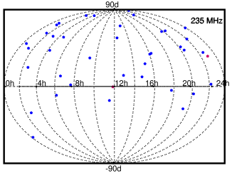
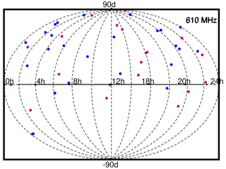
Figure 1: A Mollweide projection plot in equatorial coordinates showing the sky distribution of sources at 235 MHz (left-hand panel) and at 610 MHz (right-hand panel). The horizontal and vertical axes in each panel are right ascension and declination, respectively. The legends in the plots, i.e., red and blue points, correspond to the quality factor, good, ‘G’ and moderate, ‘M’, respectively (see Sect. 5.1) of the calibration source.

5.2 Sky Distribution

The distribution of these phase calibration radio sources on the sky reflects the structure of the observable universe on the largest possible scales that can be mapped with the GMRT via the phase-referencing technique. Fig. 1 shows the distribution of phase calibration sources on the celestial sphere. The smallest and the largest angular separations between any two phase calibration sources are $\sim$0.5 deg and $\sim$52 deg, respectively. Thus, it is possible that for a certain observation the target source may be as far as $\sim$26 deg from the nearest phase calibration source. Although Fig. 1 suggests the distribution of phase calibration sources looks patchy, there are no visible large voids in the sky. In order to provide support to this suggestion, we test the hypothesis that these phase calibration sources are randomly distributed in the sky, and hence the right ascension and sin($\pi/2-{\rm declination}$) plane will be uniformly distributed. We constructed a Halton sequence of size equal to the number of calibration sources. The Halton sequence is a deterministic sequence that produces well-spaced, uniformly distributed data, and we call this uniformly distributed sequence over the right ascension and sin($\pi/2-{\rm declination}$) plane the null distribution. We compute the gap statistics (Tibshirani, Walther & Hastie, 2000), a method for estimating the number of clusters or its nature of distribution in a set of data. Mathematically, let us consider $n$ uniform data points in $p$ dimensions, with $k$ centres, which align themselves in an equally spaced manner; then

$$\Sigma~{}{\rm log}(W_{k})\simeq{\rm log}(pn/12)-(2/p)~{}{\rm log}(k)+{\rm constant},$$

where $\Sigma~{}{\rm log}(W_{k})$ is the expectation of the error measure, log $(W_{k})$. Normalizing the graph of log $(W_{k})$ by comparing it with its expectation under the null distribution of the data gives a quantitative estimate of the uniform nature of observed distribution of phase calibration sources. We compared the gap statistics from observed and expected distributions of data and found the observed and expected curve are very close and the gap estimate is unity, suggesting uniform distribution of phase calibration sources. Alternatively, the two-point correlation function is also commonly used to quantify the clustering of distribution in a set of data. Davis & Peebles (1983) defined an estimator

$$\rho=[(\eta_{R}/\eta_{D})\times(DD/DR)]-1$$

where $DD$ and $DR$ are counts of pairs of sources (in bins of separation) in the set of observed data distribution and between the set of observed data and set of null data distributions, and $\eta_{D}$ and $\eta_{R}$ are the mean number densities of sources in the observed data and null data distributions, respectively. We find $<\rho>\simeq-0.008$ between the observed distribution of phase calibration sources and the null distribution constructed using the Halton sequence, again suggesting uniform distribution of phase calibration sources, i.e., the right ascension and sin($\pi/2-{\rm declination}$) plane is uniformly distributed.

Recall that the observations of phase calibration sources are important for (i) tracking the instrumental and the atmospheric gains, (ii) monitoring the quality and sensitivity of the data and (iii) spotting the occasional amplitude and phase jumps. Hence one chooses the calibration source closest to the target source to better calibrate atmospheric gain fluctuations. The sky distribution discussed here suggests that the phase calibration sources are uniformly distributed, but presently when making a choice with this database of calibration sources, the calibration source and the target source may have relatively large, $>$ 20 deg angular separation than the recommended proximity between the calibration source and the target source (VLA observational status summary, 2017); clearly, our ongoing efforts to increase the size of the database would address this concern.

5.3 Comparison to a Conventional Image

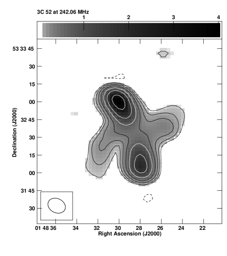
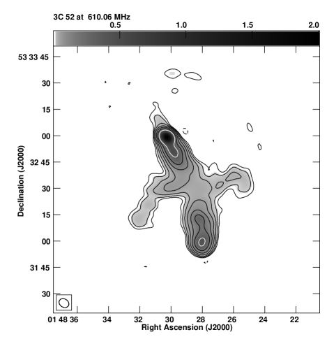
Figure 2: Upper panel: full synthesis GMRT maps of 3C 52 at 235 MHz (left-hand panel) and 610 MHz (right-hand panel). The data are reduced using the image model from the database to obtain the calibration for the secondary phase calibration source; the data reduction recipe is explained in Sect. 5.3. The synthesized beams for 235 MHz and 610 MHz are 15^′′.33 $\times$ 11^′′.92 at a P.A. of 64^∘.46 and 5^′′.92 $\times$ 4^′′.68 at a P.A. of 58^∘.35, respectively. The peak surface brightness and the RMS noises in the immediate vicinity of the source for 235 MHz and 610 MHz maps are 4.0 Jy beam^-1 and 2.0 Jy beam^-1, and 4.9 mJy beam^-1 and 0.6 mJy beam^-1, respectively. The contour levels in these two maps are RMS noise level $\times$ $-$3, 3, 6, 12, 24, 48, 96, 192 mJy beam^-1. Lower panel: the original published, full synthesis GMRT maps of 3C 52 at 235 MHz (left-hand panel) and 610 MHz (right-hand panel), Fig 2, upper-panel images of Lal & Rao (2007). The synthesized beams for 235 MHz and 610 MHz maps are 15^′′.4 $\times$ 12^′′.0 at a P.A. of 63^∘.7 and 5^′′.9 $\times$ 4^′′.7 at a P.A. of 57^∘.5, respectively; and the contour levels in the two maps are, respectively, $-$50, 50, 60, 80, 100, 160, 200, 400, 600, 800, 1200, 1600, 1800 mJy beam^-1 and $-$8, 8, 20, 30, 40, 50, 60, 80, 100, 200 mJy beam^-1, The error-bars in the full synthesis maps found at a source free location are $\sim$1.4 mJy beam^-1 and $\sim$0.3 mJy beam^-1 at 235 and 610 MHz, respectively.

In order to test our methodology, we performed data reduction in aips using standard procedures (see Sect. 4.1), but using the appropriate model image file from the database. We typically run following steps during the standard data reduction procedures, namely,

• loading the FITS file (task fitld),

• entering the absolute flux density of the primary calibration source (task setjy),

• determining calibration for the scans of primary flux density and secondary phase calibration sources (task calib),

• bootstrapping the flux density (task getjy),

• interpolating the gains (task clcal),

• perform bandpass calibration (task bpass), and

• making image of the target source (task imagr).

Instead, we used the model image file from the database to determine calibration for primary and secondary calibration sources, hence, step (3) mentioned above, was performed via. following two steps,

• solve for the antenna-based gains for primary flux density calibration source, and

• use the image model from the database, either the clean-component file or the model image file, to obtain this calibration for the secondary phase calibration source, i.e., $\phi_{\rm true}^{\rm c}$;

and rest of the data reduction steps were performed in the usual standard manner.

As a case study, we made an image of the source 3C 52 (project code 03DVL01, observing date 12 January 2003) using a image model from the database for 0110$+$565 phase calibration source of moderate M quality (see Table 2) and compared it with the image published in Lal & Rao (2007). The upper-panel of Fig. 2 shows the radio images at 235 MHz and 610 MHz using image model of phase-calibration source 0110$+$565 from the database, while the lower-panel shows the original published image (Fig 2: Lal & Rao, 2007). Clearly, we reproduce all morphological details at both these frequencies. To make further comparisons of the two images, we made difference images, subtracting upper-panel images from the corresponding lower-panel original published images (Fig. 2), at both these frequencies after matching their angular resolutions, and the RMS difference in the resultant maps was less than 4% and 3% at 235 MHz and 610 MHz, respectively. We performed similar analysis on several radio galaxies published in earlier papers e.g., Lal & Rao (2007); Lal, Hardcastle & Kraft (2008) and the RMS difference in the resultant maps was always $\lesssim$4%. We conclude that the methodology is robust and does not suffer from any systematics; thereby providing us confidence in using the image model from the database to perform phase calibration and thus fully exploiting the technique of phase-referencing.

Presently, for pulsar observations, the calibration source is used as a point source for phasing the array using an observatory based tool, rantsol. rantsol processes the raw telescope format data in real-time and determines the calibration to be applied on to the data given a model of the calibration source in order to phase the array. The output data stream would have these corrections applied. Hence only a handful of bright, P-class or S-class VLA calibration sources with flux densities more than a few Jansky are used at the observatory. Instead, a suitable image model from the GMRT calibrator database can be used to obtain antenna based solutions for all antennas. These antenna solutions would thus allow the phasing of the GMRT array for further processing by the pulsar receiver system.

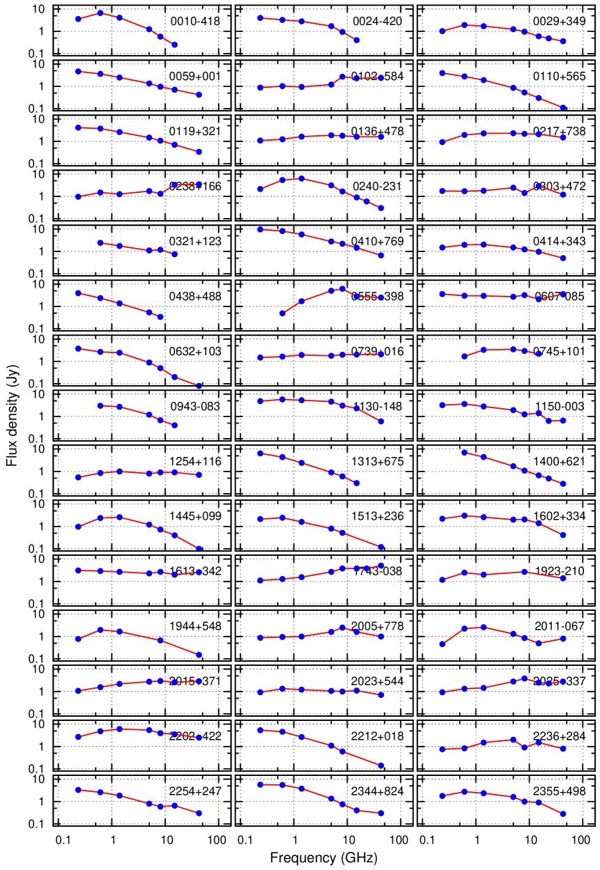
Figure 3: Integrated flux density (spectra) for the calibration sources. Various measurements along with error bars (not plotted) at 235 MHz and 610 MHz are explained in Table 2.

5.4 Integrated Radio Spectra

Table 3: Shapes of spectra for the three categories of phase calibration sources.

	Straight	Curved	Complex
Galaxies	0119$+$321, 0410$+$769, 0943$-$083,	0010$-$418, 0029$+$349, 0745$+$101,	2011$-$067, 2344$+$824, 2355$+$498
	1313$+$675, 1400$+$621, 2212$+$018	1130$-$148, 1445$+$099, 1602$+$334,
		1944$+$548
Quasars	0059$+$001, 0136$+$478, 0607$-$085,	0024$-$420, 0217$+$738, 0240$-$231,	0102$+$584, 0238$+$166, 0303$+$472,
	0739$+$016, 1613$+$342, 1743$-$038,	0414$+$343, 2202$+$422	0555$+$398, 1150$-$003, 1254$+$116,
	2015$+$371		1923$-$210, 2005$+$778, 2025$+$337,
			2236$+$284, 2254$+$247
Unidentified	0110$+$565, 0321$+$123, 0438$+$488,	1513$+$236	0632$+$103
	2023$+$544

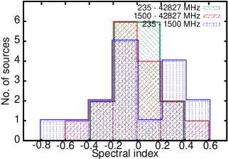
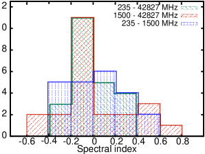
Figure 4: Histograms showing the distribution of spectral indices for calibration sources (a) at low frequencies, $\lesssim$ 1500 MHz (blue), (b) at high frequencies $\gtrsim$ 1500 MHz (red), and (c) over a complete frequency range from 235 MHz to 42.83 GHz (green) for all 45 phase calibration sources. (The borders are shifted to avoid overlapping lines and hence, for clarity.) Three panels correspond to radio galaxies (left-hand panel), quasars (middle-panel) and the unidentified sources (right-hand panel).

Determining the radio spectra of phase calibration sources is important to understand their nature and more importantly flux density scales. We analysed the integrated radio spectra of phase calibration sources by complementing the GMRT measurements at 235 MHz and 610 MHz with flux densities at other frequencies available in literature. Since all the sample phase calibration sources are unresolved; the flux densities have been determined using aips task jmfit. The integrated spectra are reported in Table 2. In Fig. 3, we present the plots of the integrated radio spectra along with a power law fit to the data. To a large extent, the GMRT measurements agree both with the fit and with the adjacent data points taken from the VLA calibrator manual (2016) database, thus providing confidence in the flux density scale in our images.

It is clear that there is considerable variety in the spectral shapes. Based on these spectral shapes (Kellermann, Pauliny-Toth & Williams, 1969), the spectra are qualitatively classified as: (i) straight, (ii) curved, both concave or convex and (iii) complex. These categories are the same as those defined by Laing & Peacock (1980); Kellermann, Pauliny-Toth & Williams (1969); Kuhr et al. (1981) in their study of radio loud quasars and radio galaxies. Briefly, sources showing straight spectra have a simple power law over the whole frequency range, sources showing curved, concave or convex spectra have positive or negative curvature, respectively, and sources showing complex spectra are thought to be the result of two or more components with different spectra. Table 3 summarizes various classes of radio spectra for these calibration sources and their radio spectra are illustrated in Fig. 3. For the straight radio spectra, the slopes tend to be steep, in the range $-1.0<\alpha<-0.5$, where $S_{\nu}\propto\nu^{\alpha}$, and $S_{\nu}$ and $\nu$ are flux density and frequency, respectively. Whenever the different components of a curved or a complex source have significantly different spectral indices, the net spectrum shows positive curvature. This suggests that when a source is made up of several components, the spectral indices and hence the electron-energy distribution of the various components are usually similar. Three sources, 1150$-$003, 1923$-$210 and 2005$+$778, all quasars, the spectra are extremely complex with several maxima and minima. Such spectra are shown by variable radio sources (Kellermann & Pauliny-Toth, 1969) and are probably the sum of a number of components each of which has a spectral cutoff at a different frequency.

Since there is no clear simple form that can be used to represent all radio spectra, we therefore fit the spectrum of each source over two ranges of frequency and a complete range of frequency. Fig. 4 shows histograms of the distribution of spectral indices for three categories, radio galaxies, quasars and the unidentified, of calibration sources at low frequencies $\lesssim$ 1500 MHz, high frequencies $\gtrsim$ 1500 MHz and over a complete frequency range from 235 MHz to 42.83 GHz. We also provide mean spectral index and dispersion for the groups of sources in Table 4 for these ranges of frequency. A summary of shapes of radio spectra and their associations with the categories of sources are as follows:

• The spectra are about equally divided between straight, curved (either concave or convex) and complex shapes.

• Quasars tend to exhibit flatter radio spectra as compared to the radio galaxies or the unidentified sources, both at low ($\lesssim$ 1500 MHz) and at high ($\gtrsim$ 1500 MHz) frequencies (see Table 4). This difference is possible because quasars have small, $<$ 1 arcsec angular diameters and in these sources synchrotron self-absorption has made a major contribution to the flattening of the spectrum at low frequencies.

• Quasars are known to be radio variable and hence possibly show complex spectra more frequently.

• Radio galaxies are found to have systematically steeper spectra than either the quasars or the unidentified sources. The steeper spectra are possibly either due to the spectral ageing of synchrotron-emitting radio lobes or due to the large redshift of distant galaxies causing the shift of the spectrum to lower frequencies.

Table 4: Mean spectral index and dispersion for the groups of sources.

	240–1500 MHz	1500–42827 MHz	240–42875 MHz
Galaxies	$<\alpha>=~{}0.03\pm 0.18$	$<\alpha>=-0.61\pm 0.06$	$<\alpha>=-0.31\pm 0.10$
Quasars	$<\alpha>=~{}0.19\pm 0.09$	$<\alpha>=-0.13\pm 0.09$	$<\alpha>=-0.02\pm 0.07$
Unidentified	$<\alpha>=-0.27\pm 0.09$	$<\alpha>=-0.57\pm 0.05$	$<\alpha>=-0.38\pm 0.10$

Note that there is evidence for time variability in the radio emission from some calibration sources (Barvainis et al., 2005), in particular the quasars, which are known to show radio variability, one must be cautious in interpreting non-simultaneous radio flux density data. Furthermore, it is unlikely that the time variability is an issue at GMRT frequencies because it is the compact core emission that shows time variability, but the low frequency emission is dominated by extended, low-surface brightness, diffuse emission, which has steeper spectra and does not show time variability (Lal, 2009, 2015; Laing & Peacock, 1980). In addition, the LOFAR Multifrequency Snapshot Sky Survey (MSSS, Heald et al., 2015) and the GaLactic and Extragalactic All-Sky MWA Survey (GLEAM, Wayth et al., 2015) would constrain the spectral properties of these calibration sources. However, the motivation of the paper is to build a database of low frequency GMRT calibrator manual, and therefore the presence or absence of time variability is not an issue as long as models for calibration sources do not change, since we use these models to determine the phase calibration for the secondary phase calibration sources.

6 Summary

It is well known that the technique of phase referencing permits the coherence time of the target source data to be extended across the entire observation (many hours). This means that the sensitivity of the observations continue to scale as the square-root of the integration-time. Here, we have introduced and made available a database of phase calibration sources for the GMRT. We provide their flux densities, models, ($u,v$) plots, final deconvolved restored maps and clean-component lists/files covering fields-of-view of $\sim$4 deg² and $\sim$0.5 deg² at 235 MHz and 610 MHz, respectively, for use in the aips and the casa for all phase calibration sources in the database. We also assign a quality factor for each of the calibration sources. The data products are available through the GMRT observatory website. A screen-shot of the GMRT calibrator manual from the online web-page is shown in Fig. 5. Additional findings from this study are:

• The distribution of these 45 phase calibration sources in the sky is uniform with no visible large gaps or voids in the sky. We used the gap statistics and the two-point correlation function to demonstrate that the distribution of phase calibration sources are random and the right ascension and sin($\pi/2-{\rm declination}$) plane is uniformly distributed. Our ongoing efforts to increase the size of this database would often provide a suitable choice of a phase calibration source that is within 20 deg to a given target source.

• Radio spectra have a variety of shapes, straight, curved and complex. We find that the relative frequencies of different shapes are nearly equal between straight, curved and complex shapes.

• Quasars tend to exhibit flatter radio spectra as compared to the radio galaxies or the unidentified sources.

• Quasars are also known to be radio variable and hence possibly tend to show complex spectra more frequently.

• Radio galaxies tend to have steeper spectra than either the quasars or the unidentified sources. The steeper spectra are possibly either due to the spectral ageing of synchrotron-emitting radio lobes or due to the large redshift of distant galaxies causing the shift of the spectrum to lower frequencies.

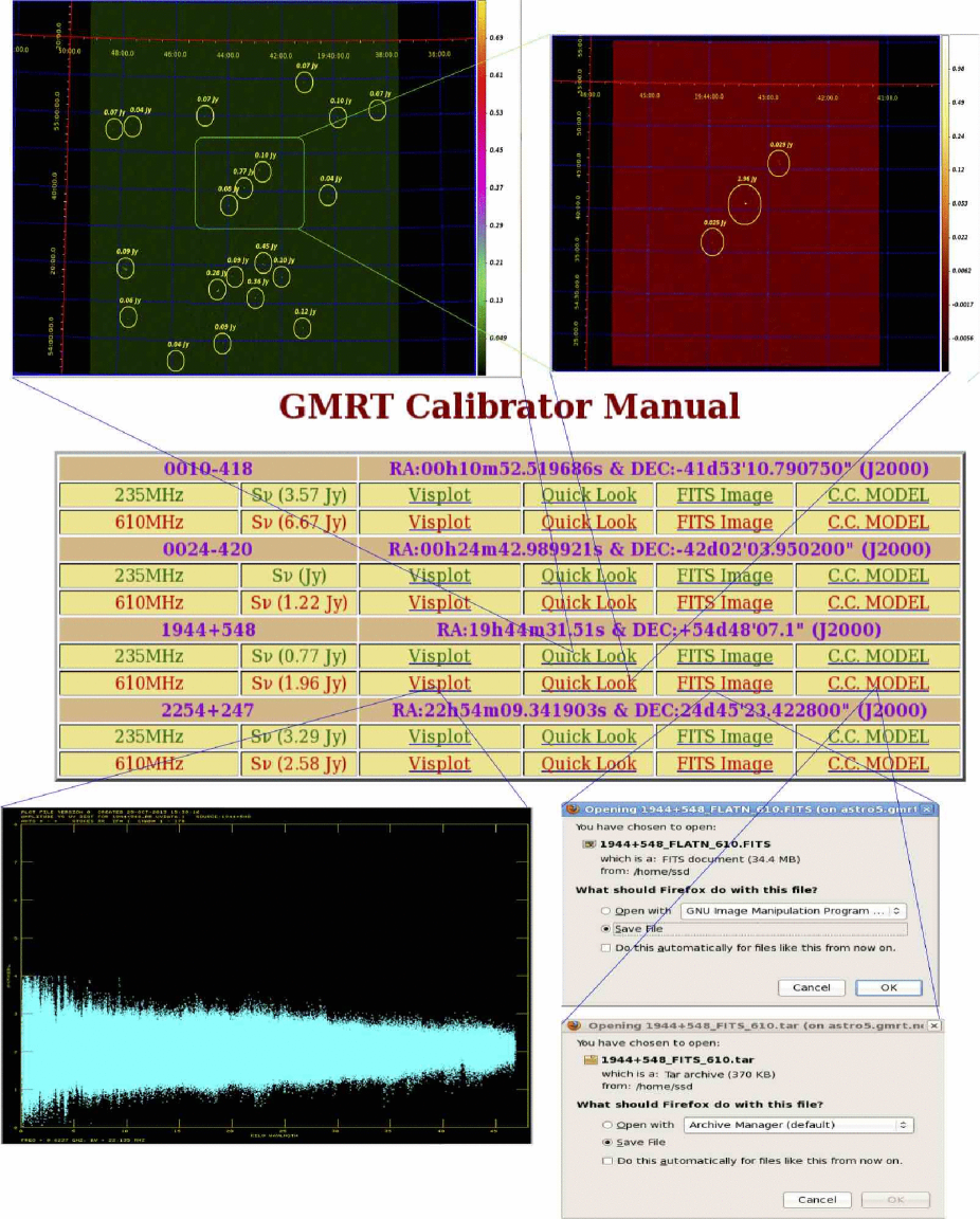
Figure 5: A screen-shot of the GMRT calibrator manual from the online web-page at the GMRT observatory. Top-left panel and top-right are the images of a calibration source at 235 MHz and 610 MHz. All the data products for a calibration source are also listed, including coordinates ($\alpha$, $\delta$), observing frequency, flux density, ($u,v$) plot (or visplot), quick-look image of the field-of-view, clean restored model map and clean-component model.

GMRT study of science target sources using calibration sources suitably chosen from the database is an effective way to determine the phase calibration for the secondary phase calibration sources and exploit fully the technique of phase-referencing. We believe this is a valuable database (available at http://gmrt.ncra.tifr.res.in) in planning a GMRT observation, be it spectral-line or continuum or pulsar. Our ongoing and future efforts will increase the size of this database, thereby allowing the user to have a larger number of calibration sources. The database at these two frequencies along with MSSS (Heald et al., 2015) and GLEAM-survey (Wayth et al., 2015) also help to interpolate the information at 325 MHz. 325 MHz band is another GMRT frequency band with very little information with regard to appropriate choices of suitable phase calibration sources. This database would also be useful at the new low-frequency bands of the upgraded GMRT (Gupta, 2016).