Study of Buffer-Aided Distributed Space-Time Coding for Cooperative Wireless Networks

Abstract

This work proposes adaptive buffer-aided distributed space-time coding schemes and algorithms with feedback for wireless networks equipped with buffer-aided relays. The proposed schemes employ a maximum likelihood receiver at the destination and adjustable codes subject to a power constraint with an amplify-and-forward cooperative strategy at the relays. Each relay is equipped with a buffer and is capable of storing blocks of received symbols and forwarding the data to the destination if selected. Different antenna configurations and wireless channels, such as static block fading channels, are considered. The effects of using buffer-aided relays to improve the bit error rate (BER) performance are also studied. Adjustable relay selection and optimization algorithms that exploit the extra degrees of freedom of relays equipped with buffers are developed to improve the BER performance. We also analyze the pairwise error probability and diversity of the system when using the proposed schemes and algorithms in a cooperative network. Simulation results show that the proposed schemes and algorithms obtain performance gains over previously reported techniques.

I Introduction

Cooperative relaying systems, which employ relay nodes with an arbitrary number of antennas between the source node and the destination node as a distributed antenna array, can obtain diversity gains by employing space-time coding (STC) schemes to improve the reliability of wireless links [1, 7]. In existing cooperative relaying systems, amplify-and-forward (AF), decode-and-forward (DF) or compress-and-forward (CF) [1] cooperation strategies are often employed with the help of multiple relay nodes.

The adoption of distributed space-time coding (DSTC) schemes at relay nodes in a cooperative network, providing more copies of the desired symbols at the destination node, can offer the system diversity and coding gains which enable more effective interference mitigation and enhanced performance. A recent focus of DSTC techniques lies in the design of full-diversity schemes with minimum outage probability [2]-[6]. In [2], the GABBA STC scheme has been extended to a distributed multiple-input and multiple-output (MIMO) network with full-diversity and full-rate, while an optimal algorithm for the design of DSTC schemes that achieve the optimal diversity and multiplexing tradeoff has been derived in [3]. A quasi-orthogonal distributed space-time block coding (DSTBC) scheme for cooperative MIMO networks is presented and shown to achieve full rate and full diversity with any number of antennas in [6]. In [19], an STC scheme that multiplies a randomized matrix by the STC code matrix at the relay node before the transmission is derived and analyzed. The randomized space-time coding (RSTC) schemes can achieve the performance of a centralized STC scheme in terms of coding gain and diversity order.

Relay selection algorithms such as those designed in [7, 8] provide an efficient way to assist the communication between the source node and the destination node. Although the best relay node can be selected according to different optimization criteria, conventional relay selection algorithms often focus on the best relay selection (BRS) scheme [9], which selects the links with maximum instantaneous signal-to-noise ratio ($SNR$). The best relay forwards the information to the destination which results in an improved BER performance. Recently, cooperative schemes with more general configurations involving a source node, a destination node and multiple relays equipped with buffers has been introduced and analyzed in [10]-[17]. The main idea is to select the best link during each time slot according to different criteria, such as maximum instantaneous $SNR$ and maximum throughput. In [10], an introduction to buffer-aided relaying networks is given, and further analysis of the throughput and diversity gain is provided in [11]. In [12] and [13], an adaptive link selection protocol with buffer-aided relays is proposed and an analysis of the network throughput and the outage probability is developed. A max-link relay selection scheme focusing on achieving full diversity gain, which selects the strongest link in each time slot is proposed in [14]. A max-max relay selection algorithm is proposed in [16] and has been extended to mimic a full-duplex relaying scheme in [15] with the help of buffer-aided relays.

Despite the early work with buffer-aided relays and its performance advantages, schemes that employ STC techniques have not been considered so far. In particular, STC and DSTC schemes encoded at the relays can provide higher diversity order and higher reliability for wireless systems. In this work, we propose adjustable buffer-aided distributed and non-distributed STC schemes, relay selection and adaptive buffer-aided relaying optimization (ABARO) algorithms for cooperative relaying systems with feedback. We examine two basic configurations of relays with STC and DSTC schemes: one in which the coding is performed independently at the relays [19], denoted multiple-antenna system (MAS) configuration, and another in which coding is performed across the relays [6], called single-antenna system (SAS) configuration. According to the literature, STC schemes can be implemented at a single relay node with multiple antennas and DSTC schemes can be used at multiple relay nodes with a single antenna. Moreover, an adjustable STC scheme is developed in [94] which indicates that by using an adjustable coding vector at single-antenna relay nodes, a complete STC scheme can be implemented. In this work, we consider a STC scheme implemented at a multiple-antenna relay node and a DSTC scheme applied at a group of single-antenna relay nodes along with adjustable STC and DSTC schemes at both types of relays. Compared to relays without buffers, buffer-aided relays help mitigate deep fading periods during communication between devices as the received symbols can be stored at the relays, which contributes to a significant BER performance improvement. Although the delay is a key issue for buffer-aided relays, their key advantage is to improve the error tolerance and transmission accuracy of the links in the network. Buffer-aided relay schemes can be used in networks in which the delay is not an issue and with delay tolerance.

The proposed schemes, relay selection and ABARO optimization algorithms can be structured into two parts, the first one is the relay selection part which chooses the best link with the maximum instantaneous $SNR$ or signal to interference and noise ratio ($SINR$) and checks if the state of the best relay node is available to transmit or receive, and the second part refers to the optimization of the adjustable STC schemes employed at the relay nodes. ABARO is based on the maximum-likelihood (ML) criterion subject to constraints on the transmitted power at the relays for different cooperative systems. STC schemes are employed at each relay node and an ML detector is employed at the destination node in order to ensure full receive diversity. Suboptimal receive and beamforming approaches [81, 82, 83, 84, 85, 86, 87, 88, 89, 90, 91, 92, 93, 94, 95, 96, 97, 98, 99, 100, 101, 102, 104, 105, 106, 107, 108, 109, 110], [111, 112, 113, 114, 115, 116, 117, 122, 119, 120, 121, 125, 122, 123, 124, 126, 127, 128, 129]. and advanced signal processing techniques [28, 29, 30, 31, 32, 33, 34, 35, 49, 37, 38, 39, 40, 41, 42, 43, 44, 45, 46, 47, 48, 49, 50, 51, 52, 53, 54, 55, 56, 60, 58, 59, 60, 61, 62, 63, 64, 65, 66, 67, 68, 69, 70, 71, 72, 73, 74, 75, 76, 77, 78, 79, 80]. can be also used at the destination node to reduce the detection complexity. Moreover, stochastic gradient (SG) adaptive algorithms [18] are developed in order to compute the required parameters at a reduced computational complexity. We study how the adjustable codes can be employed at buffer-aided relays combined with relay selection and how to optimize the adjustable codes by employing an ML criterion. A feedback channel is required in the proposed scheme and algorithms. All the computations are done at the destination node so that the useful information, such as relay selection information and optimized coding matrices are assumed known. We have studied the impact of feedback errors in [94], however, in this work we focus on the effects of using the proposed buffer-aided relay schemes, relay selection and optimization algorithms. The feedback is assumed to be error-free and the devices are assumed to have perfect channel state information (CSI). The proposed relay selection and optimization algorithms can be implemented with different types of STC and DSTC schemes in cooperative relaying systems with DF or AF protocols. We first study the design of adjustable STC schemes and relay selection algorithms for single-antenna systems and then extend it to multiple-antenna systems, which enable further diversity gains or multiplexing gains. The proposed algorithms and schemes are also considered with DSTC schemes. In single-antenna networks, DSTC schemes are used with an arbitrary number of relays and a group of relays is selected to implement the DSTC scheme. In multiple-antenna networks, a complete DSTC scheme can be obtained at each relay node and a superposition of multiple DSTC transmissions is received at the destination.

This paper is organized as follows. Section II introduces a cooperative two-hop relaying systems with multiple buffer-aided relays applying the AF strategy in SAS and MAS configurations, respectively. In Section III the detailed adjustable STC scheme is introduced. The proposed relay selection and code optimization algorithms are derived in Section IV and the DSTC schemes are considered in Section V. The analysis of the proposed algorithms is shown in Section VI, whereas in Section VII we provide the simulation results. Section VIII gives the conclusions of the work.

Notation: the italic, the bold lower-case and the bold upper-case letters denote scalars, vectors and matrices, respectively. The operator $\parallel{\boldsymbol{X}}\parallel_{F}=\sqrt{{\rm Tr}({\boldsymbol{X}}^{H}\cdot{\boldsymbol{X}})}=\sqrt{{\rm Tr}({\boldsymbol{X}}\cdot{\boldsymbol{X}}^{\emph{H}})}$ is the Frobenius norm. ${\rm Tr}(\cdot)$ stands for the trace of a matrix, and the $N\times N$ identity matrix is written as ${\boldsymbol{I}}_{N}$.

II Cooperative System Models

In this section, we introduce the cooperative system models adopted to evaluate the proposed schemes and algorithms. We consider two relay configurations: SAS in which each node contains only a single antenna and MAS in which each node contains multiple antennas. This work focuses on the relay selection and adjustable code matrices optimization algorithms so that we assume that perfect CSI is available at the relays and destination nodes. However, we remark that that CSI can be obtained in practice by using pilot sequences and cooperative channel estimation algorithms [91, 22].

II-A Cooperative System Models for SAS

Figure 1: Cooperative System Model with $n_{r}$ Relay Nodes

In this section, we consider a two-hop system that is shown in Fig.1 and which consists of a source node, a destination node and $n_{r}$ relays. Each node contains a single antenna. Let ${\boldsymbol{s}}[j]$ denote a block of modulated data symbols with length of $M$ and covariance matrix $E\big{[}{\boldsymbol{s}}[j]{\boldsymbol{s}}^{\emph{H}}[j]\big{]}=\sigma_{s}^{2}{\boldsymbol{I}}_{M}$, where $\sigma_{s}^{2}$ denotes the signal power and $j$ is the index of the blocks. We assume that the channels are static over the transmission period of ${\boldsymbol{s}}[j]$. The minimum buffer size is equal to the size of one block of symbols, $M$, and the maximum buffer size is equal to $MJ$, where $J$ is the maximum number of symbol blocks. In the first hop, the source node sends the modulated symbol vector $\boldsymbol{s}[j]$ to the relay nodes and the received data are given by

$$\boldsymbol{r}_{SR_{k}}[j] =\sqrt{P_{S}}f_{SR_{k}}[j]\boldsymbol{s}[j]+\boldsymbol{n}_{SR_{k}}[j],~{}k=1,2,...,n_{r},~{}j=1,2,...J,$$ (1)

where $f_{SR_{k}}[j]$ denotes the channel state information (CSI) between the source node and the $k$th relay, and $\boldsymbol{n}_{SR_{k}}[j]$ stands for the $M\times 1$ additive white Gaussian noise (AWGN) vector generated at the $k$th relay with variance $\sigma^{2}_{r}$. The transmission power assigned at the source node is denoted as $P_{S}$. At the relay nodes, in order to implement an STC scheme the received symbols are divided into $i=M/N$ groups, where $N$ denotes the number of symbols required to encode an STC scheme and whose value is different according to different STC schemes, e.g. $N=2$ for the $2\times 2$ Alamouti STBC scheme and $N=4$ for the linear dispersion code (LDC) scheme in [23]. The transmission in the second hop is expressed as follows:

$$\boldsymbol{r}_{R_{k}D}[i] =\sqrt{P_{R}}g_{R_{k}D}[i]{\boldsymbol{c}}_{rand}[i]+\boldsymbol{n}_{R_{k}D}[i],~{}k=1,2,...,n_{r},~{}i=1,2,...,M/N,$$ (2)

where $\boldsymbol{r}_{R_{k}D}[i]$ denotes the $i$th $T\times 1$ received symbol vector. The $T\times 1$ adjustable STC scheme is denoted by ${\boldsymbol{c}}_{rand}[i]$, and $g_{R_{k}D}[i]$ denotes the CSI factor between the $k$th relay and the destination node. The transmission power assigned at the relay node is denoted as $P_{R}$. The vector $\boldsymbol{n}_{R_{k}D}[i]$ stands for the AWGN vector generated at the destination node with variance $\sigma^{2}_{d}$. It is worth mentioning that during the transmission period of each group the channel is static. The details of adjustable STC encoding and decoding procedures are given in the next section.

II-B Cooperative System Models for MAS

Figure 2: Cooperative System Model with $n_{r}$ Relay Nodes

In this section, we extend the single-antenna system model to a two-hop multiple-antenna system that is shown in Fig.2. Each node contains $N\geq 2$ antennas. Let ${\boldsymbol{s}}[j]$ denote a modulated data symbol vector with length $M$, which is a block of symbols in a packet. The data symbol vector ${\boldsymbol{s}}[j]$ can be sent from the source to the relays within one time slot since multiple antennas are employed. We assume that the channels are static over the transmission period of ${\boldsymbol{s}}[j]$ and, for simplicity, we assume that $N=M$ and the minimum buffer size is equal to $M$. In the first hop, the source node sends ${\boldsymbol{s}}[j]$ to the relay nodes and the received data are described by

$$\boldsymbol{r}_{SR_{k}}[j] =\sqrt{\frac{P_{S}}{N}}\boldsymbol{F}_{SR_{k}}\boldsymbol{s}[j]+\boldsymbol{n}_{SR_{k}}[j],~{}k=1,2,...,n_{r},~{}j=1,2,...J,$$ (3)

where $\boldsymbol{F}_{SR_{k}}[j]$ denotes the $N\times N$ CSI matrix between the source node and the $k$th relay, and $\boldsymbol{n}_{SR_{k}}[j]$ stands for the $N\times 1$ AWGN vector generated at the $k$th relay with variance $\sigma^{2}_{r}$. At each relay node, an adjustable code vector is randomly generated before the forwarding procedure and the received data are expressed as

$${\boldsymbol{R}}_{R_{k}D}[j]=\sqrt{\frac{P_{R}}{N}}\boldsymbol{G}_{R_{k}D}[j]{\boldsymbol{V}}[j]{\boldsymbol{C}}[j]+{\boldsymbol{N}}_{R_{k}D}[j]=\sqrt{\frac{P_{R}}{N}}\boldsymbol{G}_{R_{k}D}[j]{\boldsymbol{C}}_{rand}[j]+{\boldsymbol{N}}_{R_{k}D}[j],$$ (4)

$$~{}~{}~{}~{}~{}~{}~{}~{}~{}~{}~{}~{}~{}~{}~{}~{}~{}~{}~{}~{}~{}~{}~{}~{}~{}~{}~{}k=1,2,...,n_{r},~{}j=1,2,...J,$$

where ${\boldsymbol{C}}[j]$ denotes the $N\times T$ standard STC scheme and ${\boldsymbol{V}}[j]={\rm diag}\{{\boldsymbol{v}}[j]\}$ stands for the $N\times N$ diagonal adjustable code matrix whose elements are from the adjustable vector ${\boldsymbol{v}}=[v_{1},v_{2},...,v_{N}]$. The $N\times T$ adjustable code matrix is denoted by ${\boldsymbol{C}}_{rand}[j]$. An equivalent representation of the received data is given by the received vector ${\boldsymbol{r}}_{R_{k}D}[j]$, which replaces the received symbol matrix ${\boldsymbol{R}}_{R_{k}D}[j]$ in (4) and is written as

$${\boldsymbol{r}}_{R_{k}D}[j]= \sqrt{\frac{P_{R}P_{S}}{N}}{\boldsymbol{V}}_{eq}[j]{\boldsymbol{H}}[j]{\boldsymbol{s}}[j]+\sqrt{\frac{P_{R}}{N}}{\boldsymbol{V}}_{eq}[j]{\boldsymbol{G}}_{R_{k}D}[j]{\boldsymbol{n}}_{sr_{k}}[j]+{\boldsymbol{n}}_{R_{k}D}[j]$$ (5)

$$= \sqrt{\frac{P_{R}P_{S}}{N}}{\boldsymbol{V}}_{eq}[j]{\boldsymbol{H}}[j]{\boldsymbol{s}}[j]+{\boldsymbol{n}}[j],$$

where ${\boldsymbol{V}}_{eq}[j]={\boldsymbol{I}}_{T\times T}\otimes{\boldsymbol{V}}[j]$ denotes the $TN\times TN$ block diagonal equivalent adjustable code matrix and $\otimes$ is the Kronecker product, and ${\boldsymbol{H}}[j]$ stands for the equivalent channel matrix which is the combination of ${\boldsymbol{F}}_{SR_{k}}[j]$ and ${\boldsymbol{G}}_{R_{k}D}[j]$. The $TN\times 1$ vector ${\boldsymbol{n}}[i]$ contains the equivalent received noise vector at the destination node, which can be modeled as an AWGN with zero mean and covariance matrix $(\sigma^{2}_{d}+\|{\boldsymbol{V}}_{eq}[j]{\boldsymbol{G}}_{R_{k}D}[j]\|^{2}_{F}\sigma^{2}_{r}){\boldsymbol{I}}_{NT}$.

III Adjustable Space-Time Coding Scheme

In this section, we detail the adjustable STC schemes in the SAS and MAS configurations. The encoding procedure of the adjustable coding schemes as compared to standard STC and DSTC schemes is different in the SAS and the MAS configuration, and we describe them in the following.

III-A Adjustable Space-Time Coding Scheme for SAS

Here, we develop the procedure of adjustable STC for the SAS configuration. In [19] and [94], adjustable codes are employed to allow relays with a single antenna to transmit STC schemes. In the second hop, the whole packet will be forwarded to the destination node. Due to the consideration of the performance of an $N\times T$ STC scheme, the received packet is divided into $i=M/N$ groups and each group contains $N$ symbols. These $N$ symbols will be encoded by an STC generation matrix and then forwarded to the destination. For example, suppose that a packet contains $M=100$ symbols and the $2\times 2$ Alamouti space-time block coding (STBC) scheme is used at the relay nodes. We first split ${\boldsymbol{r}}_{SR_{k}}$ into $50$ groups, encode the symbols in the first group by the Alamouti STBC scheme and then multiply a $1\times 2$ randomized vector ${\boldsymbol{v}}$. The original $2\times 2$ orthogonal Alamouti STBC scheme ${\boldsymbol{C}}$ results in the following code:

$${\boldsymbol{c}}_{rand} ={\boldsymbol{v}}{\boldsymbol{C}}=\left[v_{1}~{}v_{2}\right]\left[\begin{array}[]{cc}r_{SR_{k}}1&-r^{*}_{SR_{k}}2\\ r_{SR_{k}}2&~{}r^{*}_{SR_{k}}1\end{array}\right]$$ (6)

$$=\left[v_{1}r_{SR_{k}}1+v_{2}r_{SR_{k}}2~{}~{}v_{2}r^{*}_{SR_{k}}1-v_{1}r^{*}_{SR_{k}}2\right],$$

where $r_{SR_{k}}1$ and $r_{SR_{k}}2$ are symbols in the first group, and the $1\times 2$ vector ${\boldsymbol{v}}$ denotes the randomized vector whose elements are generated randomly according to different criteria described in [19]. As shown in (6), the $2\times 2$ STBC matrix changes to a $1\times 2$ STBC vector which can be transmitted by a relay node with a single antenna in $2$ time slots. Different STC schemes such as the LDC scheme in [23] can be easily adapted to the randomized vector encoding in (6). Therefore, the transmission of the randomized STC schemes can be described as

$${\boldsymbol{r}}=\sqrt{P_{T}}h{\boldsymbol{c}}_{rand}+{\boldsymbol{n}}=\sqrt{P_{T}}h{\boldsymbol{v}}{\boldsymbol{C}}+{\boldsymbol{n}},$$ (7)

where $h$ denotes the channel coefficient which is assumed to be constant within the transmission time slots, and ${\boldsymbol{n}}$ stands for the noise vector. The decoding methods of the randomized STC schemes are the same as that of the original STC schemes. At the destination, instead of the estimation of the channel coefficient $h$, the resulting composite parameter vector ${\boldsymbol{v}}h$ is estimated. As a result, the transmission of a randomized STC vector is similar to the transmission of a deterministic STC scheme over an effective channel. Taking the randomized Alamouti scheme as an example, the linear ML decoding for the information symbols $s_{1}$ and $s_{2}$ is given by

$$\tilde{s_{1}}=h^{*}_{rand1}r_{1}+h_{rand2}r^{*}_{2},~{}\tilde{s_{2}}=h^{*}_{rand2}r^{*}_{1}+h_{rand1}r^{*}_{2},$$ (8)

where $h_{rand1}$ and $h_{rand2}$ are the randomized channel coefficients in ${\boldsymbol{v}}h$. Different decoding methods can be employed in this context. In [94], optimization algorithms to compute the randomized code vector ${\boldsymbol{v}}$ are proposed in order to obtain a performance improvement.

Since the adjustable STC scheme is employed at the relay node, the received vector ${\boldsymbol{r}}_{R_{k}D}[i]$ in (2) can be rewritten as

$${\boldsymbol{r}}_{R_{k}D}[i]= \sqrt{P_{R}P_{S}}{\boldsymbol{V}}_{eq}[i]h[i]{\boldsymbol{s}}[i]+\sqrt{P_{R}}{\boldsymbol{V}}_{eq}[i]g_{R_{k}D}[i]{\boldsymbol{n}}_{sr_{k}}[i]+{\boldsymbol{n}}_{R_{k}D}[i]$$ (9)

$$= \sqrt{P_{R}P_{S}}{\boldsymbol{V}}_{eq}[i]h[i]{\boldsymbol{s}}[i]+{\boldsymbol{n}}[i],$$

where ${\boldsymbol{V}}_{eq}[i]$ denotes the $T\times N$ block diagonal equivalent adjustable code matrix, and $h[i]=f_{SR_{k}}[i]g_{R_{k}D}[i]$ stands for the equivalent channel. The vector ${\boldsymbol{n}}[i]$ contains the equivalent received noise vector at the destination node, which can be modeled as an AWGN with zero mean and covariance matrix $(\sigma^{2}_{d}+\|{\boldsymbol{V}}_{eq}[i]g_{R_{k}D}[i]\|^{2}_{F}\sigma^{2}_{r}){\boldsymbol{I}}_{NT}$.

III-B Adjustable Space-Time Coding Scheme for MAS

In this section, the details of the adjustable STC encoding procedure in the MAS configuration are given. As mentioned in the previous section, we assume $M=N$ so that in the MAS configuration we do not need to divide the received symbols into different groups to implement the adjustable STC scheme. Take the $2\times 2$ Alamouti STBC scheme as an example, the adjustable STC scheme is encoded as:

$${\boldsymbol{C}}_{rand} ={\boldsymbol{V}}{\boldsymbol{C}}=\left[\begin{array}[]{cc}v_{1}&0\\ 0&v_{2}\end{array}\right]\left[\begin{array}[]{cc}r_{SR_{k}}1&-r^{*}_{SR_{k}}2\\ r_{SR_{k}}2&~{}r^{*}_{SR_{k}}1\end{array}\right]$$ (10)

$$=\left[\begin{array}[]{cc}v_{1}r_{SR_{k}}1&-v_{1}r^{*}_{SR_{k}}2\\ v_{2}r_{SR_{k}}2&v_{2}r^{*}_{SR_{k}}1\end{array}\right],$$

where $r_{SR_{k}}1$ and $r_{SR_{k}}2$ are the first symbols in the separate groups, and the $2\times 2$ matrix ${\boldsymbol{V}}$ denotes the randomized matrix whose elements at the main diagonal are generated randomly according to different criteria described in [19]. The transmission of the randomized STC schemes is described in (4) and the decoding is given in (8).

IV Adaptive Buffer-Aided STC And Relay Optimization Algorithms

In this section, the proposed ABARO algorithm in SAS is derived in detail. The optimization in MAS follows a similar procedure with different channel vectors so that we will skip the derivation. The main idea of the ABARO algorithm is to choose the best relay node which contains the highest instantaneous $SNR$ for transmission and reception in order to achieve full diversity order and higher coding gain as compared to standard STC and DSTC designs. The relay nodes are assumed to contain buffers to store the received data and forward the data to the destination over the best available channels. In addition, the best relay node is always chosen in order to enhance the detection performance at the destination. As a result, with buffer-aided relays the proposed ABARO algorithm will result in improved performance.

Before each transmission, the instantaneous $SNR$ ($SNR_{ins}$) of the $SR$ and $RD$ links are calculated at the destination and conveyed with the help of signaling and feedback channels [15]. The expressions for the instantaneous $SNR$ of the $SR$ and $RD$ links are respectively given by

$$SNR_{SR_{k}}[i]=\frac{\|f_{SR_{k}}[i]\|^{2}_{F}}{\sigma^{2}_{r}},~{}SNR_{R_{k}D}[i]=\frac{\|{\boldsymbol{V}}_{eq}[i]g_{R_{k}D}[i]\|^{2}_{F}}{\sigma^{2}_{d}},$$ (11)

and the best link is chosen according to

$$SNR_{\rm opt}[i]=\arg\max_{k,b}SNR_{{\rm ins}_{k,b}}[i],~{}k=1,2,...,n_{r},~{}b=1,2,...,B,~{}i=1,2,...,M/N,$$ (12)

where $b$ denotes the occupied number of packets in the buffer. After the best relay is determined, the transmission described in (1) and (2) is implemented. The $SNR_{ins}$ is calculated first and then the destination chooses a suitable relay which has enough room in the buffer for the incoming data. For example, if the $k$th $SR$ link is chosen but the buffer at the $k$th relay node is full, the destination node will skip this node and check the state of the buffer which has the second best link. In this case the optimal relay with maximum instantaneous $SNR$ and minimum buffer occupation at a certain $SNR$ level will be chosen for transmission.

After the detection of the first group of the received symbol vector at the destination node, the adjustable code ${\boldsymbol{v}}$ will be optimized. The constrained ML optimization problem that involves the detection of the transmitted symbols and the computation of the adjustable code matrix at the destination is written as

$$\left[\hat{\boldsymbol{s}}[i],\hat{\boldsymbol{V}}_{eq}[i]\right]=\operatornamewithlimits{argmin}_{{\boldsymbol{s}}[i],{\boldsymbol{V}}_{eq}[i]}\|{\boldsymbol{r}}[i]-\sqrt{P_{R}P_{S}}{\boldsymbol{V}}_{eq}[i]h[i]\hat{\boldsymbol{s}}[i]\|^{2},$$ (13)

$$~{}~{}~{}~{}~{}~{}~{}s.t.~{}{\rm Tr}({\boldsymbol{V}}_{eq}[i]{\boldsymbol{V}}^{\emph{H}}_{eq}[i])\leq{P_{\boldsymbol{V}}},~{}i=1,2,...,M/N,$$

where ${\boldsymbol{r}}[i]$ is the received symbol vector in the $i$th group and $\hat{\boldsymbol{s}}[i]$ denotes the detected symbol vector in the $i$th group. For example, if the number of antennas $N=4$ and the number of symbols stored at the buffer is $M=8$, we have $M/N=2$ groups of symbols to implement the adjustable STC scheme. According to the properties of the adjustable code vector, the computation of $\hat{\boldsymbol{s}}[i]$ is the same as the decoding procedure of the original STC schemes. In order to obtain the optimal code vector ${\boldsymbol{v}}[i]$, the cost function in (13) should be minimized with respect to the equivalent code matrix ${\boldsymbol{V}}_{eq}[i]$ subject to a constraint on the transmitted power. The Lagrangian expression of the optimization problem in (13) is given by

$$\mathcal{L}= \|{\boldsymbol{r}}[i]-\sqrt{P_{R}P_{S}}{\boldsymbol{V}}_{eq}[i]h[i]\hat{\boldsymbol{s}}[i]\|^{2}+\lambda(Tr({\bf V}_{\rm eq}[i]{\bf V}_{\rm eq}^{\emph{H}}[i])-P_{\boldsymbol{V}}).$$ (14)

It is worth mentioning that the power constraint expressed in (13) is ignored during the optimization of the adjustable code and in order to enforce the power constraint, we introduce a normalization procedure after the optimization which reduces the computational complexity. A stochastic gradient algorithm is used to solve the optimization algorithm in (14) with lower computational complexity as compared to least-squares algorithms which require the inversion of matrices. By taking the instantaneous gradient of $\mathcal{L}$, discarding the power constraint and equating it to zero, we obtain

$$\nabla\mathcal{L}=-\sqrt{P_{R}P_{S}}({\boldsymbol{r}}[i]-\sqrt{P_{R}P_{S}}{\boldsymbol{V}}_{eq}[i]h\hat{\boldsymbol{s}}[i])\hat{\boldsymbol{s}}^{\emph{H}}[i]h^{\emph{H}},$$ (15)

and the ABARO algorithm for the proposed scheme can be expressed as follows

$${\boldsymbol{V}}_{eq}[i+1]= {\boldsymbol{V}}_{eq}[i]-\mu\sqrt{P_{R}P_{S}}({\boldsymbol{r}}[i]-\sqrt{P_{R}P_{S}}{\boldsymbol{V}}_{eq}[i]h\hat{\boldsymbol{s}}[i])\hat{\boldsymbol{s}}^{\emph{H}}[i]h^{\emph{H}}[i],$$ (16)

where $\mu$ is the step size. After the update of the equivalent coding matrix ${\boldsymbol{V}}_{eq}$ in SAS, we can recover the original coding vector ${\boldsymbol{v}}[i]$ from the entries of the main diagonal of ${\boldsymbol{V}}_{eq}$. A normalization of the original code vector ${\boldsymbol{v}}[i]$ that circumvents the power constraint in (13) is given by

$${\boldsymbol{v}}[i+1]={\boldsymbol{v}}[i+1]\frac{P_{\boldsymbol{v}}}{\sqrt{{\boldsymbol{v}}^{\emph{H}}[i+1]{\boldsymbol{v}}[i+1]}}.$$ (17)

Similarly, the ABARO algorithm in the MAS configuration can be implemented step-by-step as shown in (11) to (17). A summary of the ABARO algorithm in the MAS configuration is shown in Table I.

TABLE I: Summary of the Adaptive Buffer-Aided Relaying Optimization Algorithm for MAS configuration

Initialization:

Empty the buffer at the relays,

for $j=1,2,...$

if $j=1$

compute: ${SNR_{SR_{k}}[j]=\frac{\|\boldsymbol{F}_{SR_{k}}[j]\|_{F}^{2}}{\sigma^{2}_{n}},~{}k=1,2,...,n_{r},}$

compare: $SNR_{opt}[j]=\arg\min_{k,b}SNR^{-1}_{{\rm ins}_{k,b}}[j],~{}k=1,2,~{}...~{},n_{r},~{}b=1,2,~{}...~{},B,$

$\boldsymbol{r}_{SR_{k}}[j]=\sqrt{\frac{P_{S}}{N}}\boldsymbol{F}_{SR_{k}}[j]\boldsymbol{s}[j]+\boldsymbol{n}_{SR_{k}}[j]$,

else

compute: ${SNR_{SR_{k}}[j]=\frac{\|\boldsymbol{F}_{SR_{k}}[j]\|_{F}^{2}}{\sigma^{2}_{n}},~{}k=1,2,...,n_{r}}$

${SNR_{R_{k}D}[j]=\frac{\|{\boldsymbol{V}}_{eq}[j]{\boldsymbol{G}}_{R_{k}D}[j]\|^{2}_{F}}{\sigma^{2}_{d}},~{}k=1,2,...,n_{r}}$,

compare: $SNR_{opt}[j]=\arg\max\{SNR_{SR_{k}}[j],SNR_{R_{k}D}[j]\}$,  $k=1,2,...,n_{r}$,

if $SNR_{max}[j]=SNR_{SR_{k}}[j]~{}\&\rm{~{}Relay_{k}~{}is~{}not~{}full}$

$\boldsymbol{r}_{SR_{k}}[j]=\sqrt{\frac{P_{S}}{N}}\boldsymbol{F}_{SR_{k}}[j]\boldsymbol{s}[j]+\boldsymbol{n}_{SR_{k}}[j]$,

elseif $SNR_{max}[j]=\arg\max SNR_{R_{k}D}[j]~{}\&\rm{~{}Relay_{k}~{}is~{}not~{}empty}$

${\boldsymbol{r}}_{R_{k}D}[j]=\sqrt{\frac{P_{R}}{N}}{\boldsymbol{V}}_{eq}[j]{\boldsymbol{H}}[j]{\boldsymbol{s}}[j]+{\boldsymbol{n}}[j]$,

ML detection:

$\hat{\boldsymbol{s}}[j]=\arg\min_{\hat{\boldsymbol{s}}[j]}\|{\boldsymbol{r}}_{R_{k}D}[j]-\sqrt{\frac{P_{R}P_{S}}{N}}{\boldsymbol{V}}_{eq}[j]{\boldsymbol{H}}[j]\hat{\boldsymbol{s}}[j]\|^{2}$,

Adjustable Matrix Optimization:

${\boldsymbol{V}}_{eq}[j+1]={\boldsymbol{V}}_{eq}[j]-\mu\sqrt{\frac{P_{R}P_{S}}{N}}({\boldsymbol{r}}_{R_{k}D}[j]-\sqrt{\frac{P_{R}P_{S}}{N}}{\boldsymbol{V}}_{eq}[j]{\boldsymbol{H}}[j]\hat{\boldsymbol{s}}[j])\hat{\boldsymbol{s}}^{\emph{H}}[j]{\boldsymbol{H}}^{\emph{H}}[j]$,

Normalization:

${\boldsymbol{V}}[j+1]={\boldsymbol{V}}[j+1]\frac{P_{\boldsymbol{V}}}{\sqrt{\|{\boldsymbol{V}}[j+1]\|_{F}^{2}}}$,

elseif $SNR_{SR_{k}}\rm{~{}is~{}max}~{}\&\rm{~{}Relay_{k}~{}is~{}full}$

skip this Relay,

elseif $SNR_{R_{k}D}\rm{~{}is~{}max}~{}\&\rm{~{}Relay_{k}~{}is~{}empty}$

skip this Relay,

…repeat…

end

end

end

V Best Relay Selection with DSTC Schemes

In this section, we assume that the relays contain buffers and employ DSTC schemes in the second hop for the SAS and MAS configurations. In particular, we also present the design of a best group relay selection algorithm for performance enhancement. The details of the deployment of DSTC schemes in the MAS configuration is similar to that in the SAS scheme. Therefore, we will not repeat it to avoid redundancy. The main difference between the relay selection algorithm for DSTC schemes as compared to that for STC schemes is due to the fact that for DSTC schemes a group of relays is selected. Specifically for DSTC schemes, the source node broadcasts data to all the relays and a DF protocol is employed at the relays. After the detection, the proposed group relay selection algorithm is employed. It is important to notice that if the DSTC schemes are used at the relays, each relay has to contain one copy of the modulated symbol vector which means in the first hop the source node cannot choose the best relay but only broadcast the symbol vector to all relays. The adjustable code vectors can be considered at each relay as well.

V-A DSTBC schemes

In this subsection, we detail the DSTBC scheme used in this study. In the SAS configuration, a single antenna is used in each node and the DF protocol is employed at the relay nodes. In the first hop, the source node broadcasts information symbol vector ${\boldsymbol{s}}$ to the relay node which is given by

$$\boldsymbol{r}_{SR_{k}}[j] =\sqrt{P_{S}}f_{SR_{k}}[j]\boldsymbol{s}[j]+\boldsymbol{n}_{SR_{k}}[j],~{}k=1,2,...,n_{r},~{}j=1,2,...,J,$$ (18)

where $\boldsymbol{s}[j]$ is a block of symbols with length of $M$, $f_{SR_{k}}[j]$ denotes the CSI and $\boldsymbol{n}_{SR_{k}}[j]$ stands for the $M\times 1$ AWGN. The transmission power assigned at the source node is denoted as $P_{S}$. After the detection at the $k$th node, $\hat{\boldsymbol{s}}_{k}$ can be obtained. The relays are then divided into $m=N_{DSTC}/n_{r}$ groups to implement the DSTC scheme, where $N_{DSTC}$ denotes the number of antennas to form the DSTC scheme. It should be noted that synchronization at the symbol level and of the carrier phase is assumed in this work. If one considers the distributed Alamouti STBC as an example, the encoding procedure is detailed in Table II, where ${\boldsymbol{s}}=[s^{(1)}_{1}$ $s^{(1)}_{2}]$ denotes the estimated symbols at relay $1$, and ${\boldsymbol{s}}=[s^{(2)}_{1}s^{(2)}_{2}]$ denotes the symbols estimated at relay $2$.

TABLE II: Distributed Alamouti in SAS

	1st Time Slot	2nd Time Slot
Relay 1	$s^{(1)}_{1}$	$-s^{(1)*}_{2}$
Relay 2	$s^{(2)}_{2}$	$-s^{(2)*}_{1}$

Note that it is assumed that the best relays will be chosen in the second hop and synchronization is perfect so after the relays forward the DSTC schemes to the destination, a composite signal comprising DSTC transmissions from multiple relays is received. The signal received in the second hop is described by

$$\boldsymbol{r}_{RD_{m}}[j] =\sum_{m=1}^{N_{DSTC}/n_{r}}\sqrt{\frac{P_{R}}{N_{DSTC}}}{\boldsymbol{g}}_{RD_{m}}[j]{\boldsymbol{C}}_{m}[j]+\boldsymbol{n}_{RD_{m}}[j],~{}j=1,2,...,M/N_{DSTC},~{}m=1,2,...,N_{DSTC}/n_{r},$$ (19)

where $\boldsymbol{r}_{RD_{m}}[j]$ denotes the $T\times 1$ received symbol matrix, and ${\boldsymbol{g}}_{RD_{m}}[j]$ denotes the $m$th channel coefficients vector. The parameter $M$ denotes the number of symbols stored in the buffers, $m$ denotes the number of relay groups to implement the DSTC scheme and $j$ denotes the DSTC scheme index.

V-B Best Relay Selection with DSTC in SAS

In this subsection, we describe the best relay selection algorithm used in conjunction with the DSTC scheme in the SAS configuration. In particular, the best relay selection algorithm is based on the techniques reported in [9] and [26], however, the approach presented here is modified for DSTC schemes and buffer-aided relay systems. In the first hop, the $M\times 1$ modulated signal vector ${\boldsymbol{s}}[j]$ is broadcast to the relays during $M$ time slots and the $M\times 1$ received symbol vector ${\boldsymbol{r}}_{SR_{k}}[j]$ is given by

$${\boldsymbol{r}}_{SR_{k}}[j]=\sqrt{P}f_{SR_{k}}[j]{\boldsymbol{s}}[j]+{\boldsymbol{n}}[j],~{}k=1,2,...,n_{r},~{}j=1,2,...,J,$$ (20)

where $f_{SR_{k}}[j]$ denotes the complex scalar channel gain between the $k$th relay and the destination, and the AWGN noise vector ${\boldsymbol{n}}[j]$ is generated at the $k$th relay node with variance equal to $\sigma^{2}_{n}$. The relays are equipped with buffers to store the received symbol vectors and the optimal relays are chosen according to the approach reported in [27] in order to implement the DSTC scheme among the relays. Specifically, all the relays will be divided into $m=\frac{N_{DSTC}}{n_{r}}$ groups and the best relay group with the highest $SINR$ will be chosen to forward the received symbols. The opportunistic relay selection algorithm is given by

$$SINR_{k}[j]=\operatornamewithlimits{argmax}_{{\boldsymbol{g}}_{RD_{k}}[j]}\frac{\|{\boldsymbol{g}}_{RD_{k}}[j]\|^{2}_{F}}{\sum_{m=1,m\neq k}^{K}\sqrt{\|{\boldsymbol{g}}_{RD_{m}}[j]\|^{2}_{F}}+\sigma^{2}_{d}},$$ (21)

where ${\boldsymbol{g}}_{RD_{m}}[j]$ denote the $1\times N_{DSTC}$ channel vector between the chosen relays and the destination to implement the DSTC scheme and $K=C_{n_{r}}^{N_{DSTC}}$ denotes all possible relay group combinations. The noise variance is given by $\sigma^{2}_{d}$. After the relay group selection, the optimal relay group transmits the DSTC signals to the destination node and the received data at the destination is described by

$$\boldsymbol{r}_{RD_{m}}[j] =\sqrt{\frac{P_{R}}{N_{DSTC}}}{\boldsymbol{g}}_{RD_{m}}[j]{\boldsymbol{C}}_{m}[j]+\boldsymbol{n}_{RD_{m}}[j],$$ (22)

where ${\boldsymbol{C}}_{m}[j]$ denotes the DSTC scheme encoded among the chosen relays. The DSTC decoding process is similar to that of the original STC scheme. It is worth mentioning that the adjustable coding schemes can be introduced in DSTC schemes and the optimization of the adjustable code vector will result in a performance improvement. The summary of the ABARO algorithm for DSTC schemes in the SAS configuration is shown in Table III.

TABLE III: Summary of the Adaptive Buffer-Aided Relaying Optimization Algorithm for DSTC Schemes in SAS

Initialization:

Empty the buffer at the relays,

for $j=1,2,...$

if $j=1$

${\boldsymbol{r}}_{SR_{k}}[j]=\sqrt{P_{S}}f_{SR_{k}}[j]{\boldsymbol{s}}[j]+{\boldsymbol{n}}[j]$,

else

compute: ${SNR_{SR_{k}}[j]=\sum_{k=1}^{n_{r}}\frac{\|f_{SR_{k}}[j]\|_{F}^{2}}{\sigma^{2}_{n}}}$,

${SNR_{R_{k}D}[j]=\sum_{k=1}^{n_{r}}\frac{\|g_{R_{k}D}[j]\|^{2}_{F}}{\sigma^{2}_{d}}}$,

compare: $SNR_{opt}[j]=\arg\max\{SNR_{SR_{k}}[j],SNR_{R_{k}D}[j]\}$,

if $SNR_{max}[j]=SNR_{SR_{k}}[j]~{}\&\rm{~{}All~{}the~{}Relays~{}are~{}not~{}full}$

$\boldsymbol{r}_{SR_{k}}[j]=\sqrt{P_{S}}f_{SR_{k}}[j]\boldsymbol{s}[j]+\boldsymbol{n}_{SR_{k}}[j]$,

elseif $SNR_{max}[j]=SNR_{R_{k}D}[j]~{}\&~{}All~{}the~{}Relays\rm{~{}are~{}not~{}empty}$

${SINR_{k}[j]=\arg\max_{{\boldsymbol{g}}_{RD_{k}}[j]}\frac{\|{\boldsymbol{g}}_{RD_{m}}[j]\|^{2}_{F}}{\sum_{m=1,m\neq k}^{K}\sqrt{\|{\boldsymbol{g}}_{RD_{m}}[j]\|^{2}_{F}}+\sigma^{2}_{d}}}$,

$\boldsymbol{r}_{R_{k}D}[j]=\sqrt{\frac{P_{R}}{N_{DSTC}}}{\boldsymbol{g}}_{R_{k}D}[j]{\boldsymbol{C}}_{k}[j]+\boldsymbol{n}_{R_{k}D}[j]$,

elseif $SNR_{SR_{k}}[j]\rm{~{}is~{}max}~{}\&~{}Relay_{k}\rm{~{}is~{}full}$

skip this Relay,

elseif $SNR_{R_{k}D}\rm{~{}is~{}max}~{}\&~{}Relay_{k}\rm{~{}is~{}empty}$

skip this Relay,

…repeat…

end

end

end

V-C Best Relay Selection with DSTC in MAS

The best relay selection algorithm described in the previous section is now extended to the MAS configuration in this subsection. The main difference between the best relay selection for SAS and MAS is the use of multiple antennas at each node. Moreover, the relays equipped with multiple antennas will obtain a complete STC scheme and only one best relay node will be chosen according to the BRS algorithm. Assuming $M=N$, each node equips $N\geq 2$ antennas and in the first hop, the $M\times 1$ modulated signal vector ${\boldsymbol{s}}[j]$ is broadcast to the relays within $1$ time slot and the $M\times 1$ received symbol matrix ${\boldsymbol{r}}_{SR_{k}}[j]$ is given by

$${\boldsymbol{r}}_{SR_{k}}[j]=\sqrt{\frac{P}{N}}{\boldsymbol{F}}_{SR_{k}}[j]{\boldsymbol{s}}[j]+{\boldsymbol{n}}[j],~{}k=1,2,...,n_{r},~{}j=1,2,...J,$$ (23)

where ${\boldsymbol{F}}_{SR_{k}}[j]$ denotes the channel coefficient matrix between the $k$th relay and the destination, and the AWGN noise vector ${\boldsymbol{n}}[j]$ is generated at the $k$th relay node with variance $\sigma^{2}_{n}$. The $N\times 1$ received symbol vector is stored at the relays and the optimal relay will be chosen according to [27]. The opportunistic relay selection algorithm for the DSTC scheme and the MAS configuration is given by

$$SNR_{k}[j]=\operatornamewithlimits{argmax}_{{\boldsymbol{G}}_{R_{k}D}[j]}\frac{\|{\boldsymbol{G}}_{R_{k}D}[j]\|^{2}_{F}}{\sigma^{2}_{d}},~{}k=1,2,...,n_{r},$$ (24)

where ${\boldsymbol{G}}_{R_{k}D}[j]$ denotes the $N\times N$ channel matrix between the $k$th relay and the destination. After the best relay with the maximum $SNR$ is chosen, the data is encoded by the DSTC scheme. The DSTC encoded and transmitted data in the second hop is received at the destination as described by

$${\boldsymbol{R}}[j]=\sqrt{\frac{P}{N}}{\boldsymbol{G}}_{R_{k}D}[j]{\boldsymbol{M}}[j]+{\boldsymbol{N}}[j],$$ (25)

where ${\boldsymbol{M}}[j]$ denotes the $N\times T$ DSTC encoded data, ${\boldsymbol{R}}[j]$ denotes the $N\times T$ received data matrix, and ${\boldsymbol{N}}[j]$ is the AWGN matrix with variance $\sigma^{2}_{d}$.

VI Analysis

In this section, we assess the computational complexity of the proposed algorithms and derive the pairwise error probability (PEP) of cooperative systems that employ adaptive STC and DSTC schemes. The expression of the PEP upper bound is adopted due to its relevance to assess STC and DSTC schemes. We also study the effects of the use of buffers and adjustable codes at the relays, and derive analytical expressions for their impact on the PEP. As mentioned in Section II, the adjustable codes are considered in the derivation as it affects the performance by reducing the upper bound of the PEP. Similarly, the buffers store the data and forward it by selecting the best available associated channel for transmission so that the performance improvement is quantified in our analysis. The PEP upper bound of the traditional STC schemes in [24] is used for comparison purposes. The main difference between the PEP upper bound in [24] and that derived in this section lies in the increase of the eigenvalues of the adjustable codes and channels which leads to higher coding gains. The derived upper bound holds for systems with different sizes and an arbitrary number of relay nodes.

VI-A Computational Complexity Analysis

According to the description of the proposed algorithms in Sections IV and V, the SG algorithms reduces the computational complexity by avoiding the channel inversion as compared to the existing algorithms. The computational complexity of the proposed SG adjustable matrix optimization in the SAS and MAS configurations is $(3+T)N$ and $(3+T)N^{2}$, respectively. The main difference between the proposed algorithms in the SAS and MAS configurations is the number of antennas. For example, the computational complexity of $SNR$ in $SR$ and $RD$ links in SAS configuration is $2N(1+T)$ according to (11), while the computational complexity of $SNR$ in $SR$ and $RD$ links in the MAS configuration is $2N^{2}(1+T)$. In addition, if a higher-level modulation scheme is employed, larger relay networks and more antennas are used at the relay node, the STC and DSTC schemes and the relay selection algorithm as well as the coding vector optimization algorithm become more complex. For example, if a $4$-antenna relay node is employed, the number of multiplications will be increased from $10$ when using a $2$-antenna relay node to $28$, and if $4$ single-antenna relay nodes are employed to implement a DSTC scheme the number of multiplications will be increased from $20$ to $112$.

VI-B Pairwise Error Probability

Consider an $N\times N$ STC scheme at the relay node with $T$ codewords. The codeword ${\boldsymbol{C}}^{1}$ is transmitted and decoded as another codeword ${\boldsymbol{C}}^{i}$ at the destination node, where $i=1,2,...,T$. According to [24], the probability of error for this code can be upper bounded by the sum of all the probabilities of incorrect decoding, which is given by

$${\rm P_{e}}\leq\sum_{i=2}^{T}{\rm P}({\boldsymbol{C}}^{1}\rightarrow{\boldsymbol{C}}^{i}).$$ (26)

Assuming that the codeword ${\boldsymbol{C}}^{2}$ is decoded at the destination node and that we know the channel information perfectly, we can derive the conditional PEP of the STC encoded with the adjustable code matrix ${\boldsymbol{V}}$ as [25]

$${\rm P}({\boldsymbol{C}}^{1}\rightarrow{\boldsymbol{C}}^{2}\mid{{\boldsymbol{V}}})={\rm Q}\left(\sqrt{\frac{\gamma}{2}}\parallel{\boldsymbol{V}}{\boldsymbol{G}}_{R_{k}D}({\boldsymbol{C}}^{1}-{\boldsymbol{C}}^{2})\parallel_{F}\right),$$ (27)

where ${\boldsymbol{G}}_{R_{k}D}$ stands for the channel coefficients matrix. Let ${\boldsymbol{U}}^{\emph{H}}{\boldsymbol{\Lambda}}_{\boldsymbol{C}}{\boldsymbol{U}}$ be the eigenvalue decomposition of $({\boldsymbol{C}}^{1}-{\boldsymbol{C}}^{2})^{\emph{H}}({\boldsymbol{C}}^{1}-{\boldsymbol{C}}^{2})$, where ${\boldsymbol{U}}$ is a unitary matrix with the eigenvectors and ${\boldsymbol{\Lambda}}_{\boldsymbol{C}}$ is a diagonal matrix which contains all the eigenvalues of the difference between two different codewords ${\boldsymbol{C}}^{1}$ and ${\boldsymbol{C}}^{2}$. Let ${\boldsymbol{Y}}^{\emph{H}}{\boldsymbol{\Lambda}}_{{\boldsymbol{G}}_{n}}{\boldsymbol{Y}}$ stand for the eigenvalue decomposition of $({\boldsymbol{G}}_{RkD}{\boldsymbol{U}})^{H}{\boldsymbol{G}}_{RkD}{\boldsymbol{U}}$, where ${\boldsymbol{Y}}$ is a unitary matrix that contains the eigenvectors and ${\boldsymbol{\Lambda}}_{\boldsymbol{V}}$ is a diagonal matrix with the eigenvalues arranged in decreasing order. The eigenvalue decomposition of $({\boldsymbol{Y}}{\boldsymbol{V}}{\boldsymbol{U}})^{\emph{H}}{\boldsymbol{Y}}{\boldsymbol{V}}{\boldsymbol{U}}$ is denoted by ${\boldsymbol{W}}^{\emph{H}}{\boldsymbol{\Lambda}}_{{\boldsymbol{V}}_{n}}{\boldsymbol{W}}$, where ${\boldsymbol{W}}$ is a unitary matrix that contains the eigenvectors and ${\boldsymbol{\Lambda}}_{{\boldsymbol{V}}_{n}}$ is a diagonal matrix with the eigenvalues. Therefore, the conditional PEP can be written as

$${\rm P}({\boldsymbol{C}}^{1}\rightarrow{\boldsymbol{C}}^{2}\mid{\boldsymbol{V}})={\rm Q}\left(\sqrt{\frac{\gamma}{2}\sum^{NT}_{m=1}\sum^{N}_{n=1}\lambda_{{\boldsymbol{V}}_{n}}\lambda^{opt}_{{\boldsymbol{G}}_{n}}\lambda_{{\boldsymbol{C}}_{n}}|\xi_{n,m}|^{2}}\right),$$ (28)

where $\xi_{n,m}$ is the $(n,m)$th element in ${\boldsymbol{Y}}$, and $\lambda_{{\boldsymbol{V}}_{n}}$, $\lambda^{opt}_{{\boldsymbol{G}}_{n}}$ and $\lambda_{{\boldsymbol{C}}_{n}}$ are the $n$th eigenvalues in ${\boldsymbol{\Lambda}}_{\boldsymbol{V}}$, ${\boldsymbol{\Lambda}}_{{\boldsymbol{G}}_{n}}$ and ${\boldsymbol{\Lambda}}_{\boldsymbol{C}}$, respectively. It is important to note that the value of $\lambda_{\boldsymbol{V}}$ and $\lambda^{opt}_{{\boldsymbol{G}}_{n}}$ are positive and real because $({\boldsymbol{G}}_{R_{k}D}{\boldsymbol{U}})^{H}{\boldsymbol{G}}_{RkD}{\boldsymbol{U}}$ and $({\boldsymbol{Y}}{\boldsymbol{V}}{\boldsymbol{U}})^{\emph{H}}{\boldsymbol{Y}}{\boldsymbol{V}}{\boldsymbol{U}}$ are Hermitian symmetric matrices. According to [24], an appropriate upper bound assumption of the ${\rm Q}$ function is ${\rm Q}(x)\leq\frac{1}{2}e^{\frac{-x^{2}}{2}}$, thus the upper bound of the PEP for an adaptive STC scheme is given by

$${\rm P}_{e_{\boldsymbol{V}}}\leq E\left[\frac{1}{2}\exp\left(-\frac{\gamma}{4}\sum^{NT}_{m=1}\sum^{N}_{n=1}\lambda_{{\boldsymbol{V}}_{n}}\lambda^{opt}_{{\boldsymbol{G}}_{n}}\lambda_{{\boldsymbol{C}}_{n}}|\xi_{n,m}|^{2}\right)\right]=\frac{1}{\prod_{n=1}^{N}(1+\frac{\gamma}{4}\lambda_{{\boldsymbol{V}}_{n}}\lambda^{opt}_{{\boldsymbol{G}}_{n}}\lambda_{{\boldsymbol{C}}_{n}})^{NT}}.$$ (29)

The key elements of the PEP are $\lambda_{{\boldsymbol{V}}_{n}}$ and $\lambda^{opt}_{{\boldsymbol{G}}_{n}}$ which related to the adjustable code matrices and the channels in the second hop. In the following subsection we will provide an analysis of these key elements separately.

VI-C Effect of Adjustable Code Matrices

Before the analysis of the effect of the adjustable code matrices, we derive the expression of the upper bound of the error probability expression for a traditional STC. It is worth mentioning that in this section, we focus on the effort of using adjustable code matrices at the relays and the relay selection and the effort of buffers are not considered.

According to [24], the PEP upper bound of the SAS configuration using traditional STC schemes is given by

$${\rm P}_{e}\leq E\left[\frac{1}{2}\exp\left(-\frac{\gamma}{4}\sum^{NT}_{m=1}\sum^{N}_{n=1}\lambda_{{\boldsymbol{C}}_{n}}|\xi_{n,m}|^{2}\right)\right]=\frac{1}{\prod_{n=1}^{N}(1+\frac{\gamma}{4}\lambda_{{\boldsymbol{C}}_{n}})^{NT}},$$ (30)

where $\lambda_{{\boldsymbol{C}}_{n}}$ denotes the $n$th eigenvalue of the distance matrix by using a traditional STC scheme. If we rearrange the terms in (30), we can rewrite the upper bound of the PEP of traditional STC scheme as

$${\rm P}_{e}\leq\left(\frac{\gamma}{4}\right)^{-N^{2}T}\prod_{n=1}^{N}\lambda^{-NT}_{{\boldsymbol{C}}_{n}}.$$ (31)

If we only consider adjustable code matrices at relays without the relay selection and buffers, the upper bound of the PEP of the proposed ABARO algorithm is derived as

$${\rm P}_{e_{\boldsymbol{V}}}\leq\frac{1}{\prod_{n=1}^{N}(1+\frac{\gamma}{4}\lambda_{{\boldsymbol{V}}_{n}}\lambda_{{\boldsymbol{C}}_{n}})^{NT}}\approx\left(\left(\frac{\gamma}{4}\right)^{-N^{2}T}\prod_{n=1}^{N}\lambda^{-NT}_{{\boldsymbol{C}}_{n}}\right)\prod_{n=1}^{N}\lambda^{-NT}_{{\boldsymbol{V}}_{n}}={\rm P}_{e}\prod_{n=1}^{N}\lambda^{-NT}_{{\boldsymbol{V}}_{n}},$$ (32)

By comparing (31) and (32), employing an adjustable code matrix for an STC scheme at the relay node introduces $\lambda_{{\boldsymbol{V}}_{n}}$ in the PEP upper bound. The adjustable code matrices are chosen according to the criterion introduced in [19] and the Hermitian matrix ${\boldsymbol{V}}^{\emph{H}}_{n}{\boldsymbol{V}}_{n}$ is positive semi-definite. With the aid of numerical tools, we have found that ${\boldsymbol{\Lambda}}_{\boldsymbol{V}}$ is diagonal with one eigenvalue less than $1$ and others much greater than $1$. We define the coding gain factor $\eta$ which denotes the quotient of the traditional STC PEP and the adjustable STC PEP as described by

$$\eta\triangleq\frac{P_{e}}{P_{e_{\boldsymbol{V}}}}=\prod_{n=1}^{N}\lambda^{NT}_{{\boldsymbol{V}}_{n}}\gg 1.$$ (33)

As a result, by using the adjustable code matrices at the relays contributes to a decrease of the BER performance. The effect of employing and optimizing the adjustable code matrix corresponds to introducing coding gain into the STC schemes. The power constraint enforced by (17) introduces no additional power and energy during the optimization. As a result, employing the adjustable code matrices in the MAS and the SAS configurations can provide a decrease in the BER upper bound since the value in the denominator increases without additional transmit power.

VI-D Effect of Buffer-aided Relays

In this subsection, the effect of using buffers at the relays is mathematically analyzed. The expression of the PEP upper bound is adopted again in this subsection. The traditional STC scheme is employed in this subsection in order to highlight the performance improvement by using buffers at the relays.

Let ${\boldsymbol{U}}^{\emph{H}}{\boldsymbol{\Lambda}}_{\boldsymbol{C}}{\boldsymbol{U}}$ be the eigenvalue decomposition of $({\boldsymbol{C}}^{1}-{\boldsymbol{C}}^{2})^{\emph{H}}({\boldsymbol{C}}^{1}-{\boldsymbol{C}}^{2})$ and ${\boldsymbol{Y}}^{\emph{H}}{\boldsymbol{\Lambda}}_{{\boldsymbol{G}}_{R_{k}D}}{\boldsymbol{Y}}$ be the eigenvalue decomposition of $({\boldsymbol{G}}_{RkD}{\boldsymbol{U}})^{H}{\boldsymbol{G}}_{RkD}{\boldsymbol{U}}$, the PEP upper bound of a traditional STC scheme in buffer-aided relays is given by

$$P_{e_{{\boldsymbol{G}}^{opt}_{n}}} \leq E\left[\frac{1}{2}\exp\left(-\frac{\gamma}{4}\sum^{NT}_{m=1}\sum^{N}_{n=1}\lambda^{opt}_{{\boldsymbol{G}}_{n}}\lambda_{{\boldsymbol{C}}_{n}}|\xi_{n,m}|^{2}\right)\right]=\frac{1}{\prod_{n=1}^{N}(1+\frac{\gamma}{4}\lambda^{opt}_{{\boldsymbol{G}}_{n}}\lambda_{{\boldsymbol{C}}_{n}})^{NT}}$$ (34)

$$\approx\left(\frac{\gamma}{4}\right)^{-N^{2}T}\prod_{n=1}^{N}\lambda^{-NT}_{{\boldsymbol{C}}_{n}}\prod_{n=1}^{N}\lambda^{-NT}_{{\boldsymbol{G}}^{opt}_{n}},$$

where $\lambda_{{\boldsymbol{C}}_{n}}$ denotes the eigenvalues of the traditional STC scheme and $\lambda_{{\boldsymbol{G}}^{opt}_{n}}$ denotes the eigenvalue of the channel components. The PEP performance of a traditional STC scheme without buffer-aided relays is given by

$$P_{e}\leq\frac{1}{\prod_{n=1}^{N}(1+\frac{\gamma}{4}\lambda_{{\boldsymbol{G}}_{n}}\lambda_{{\boldsymbol{C}}_{n}})^{NT}}\approx\left(\frac{\gamma}{4}\right)^{-N^{2}T}\prod_{n=1}^{N}\lambda^{-NT}_{{\boldsymbol{C}}_{n}}\prod_{n=1}^{N}\lambda^{-NT}_{{\boldsymbol{G}}_{n}},$$ (35)

where $\lambda_{{\boldsymbol{C}}_{n}}$ denotes the eigenvalues of the traditional STC scheme and $\lambda_{{\boldsymbol{G}}_{n}}$ denotes the eigenvalue of the channels in second hop. By comparing (34) and (35), the only difference is the product of the channel eigenvalues. To show the advantage of employing buffer-aided relays, we need to prove that $P_{e_{{\boldsymbol{G}}^{opt}_{n}}}<P_{e}$.

We can simply divide (34) by (35) and obtain

$$\beta=\frac{P_{e}}{P_{e_{{\boldsymbol{G}}^{opt}_{n}}}}=\frac{\left(\frac{\gamma}{4}\right)^{-N^{2}T}\prod_{n=1}^{N}\lambda^{-NT}_{{\boldsymbol{C}}_{n}}\prod_{n=1}^{N}\lambda^{-NT}_{{\boldsymbol{G}}_{n}}}{\left(\frac{\gamma}{4}\right)^{-N^{2}T}\prod_{n=1}^{N}\lambda^{-NT}_{{\boldsymbol{C}}_{n}}\prod_{n=1}^{N}\lambda^{-NT}_{{\boldsymbol{G}}^{opt}_{n}}}=\frac{\prod_{n=1}^{N}\lambda^{NT}_{{\boldsymbol{G}}^{opt}_{n}}}{\prod_{n=1}^{N}\lambda^{NT}_{{\boldsymbol{G}}_{n}}}.$$ (36)

As derived in Section IV, the instantaneous SNR of the channels is computed and the channel with highest SNR is chosen which contains the largest eigenvalues among all the channels. As a result, we have

$$\lambda^{opt}_{{\boldsymbol{C}}_{n}}>\lambda_{{\boldsymbol{C}}_{n}},n=1,2,...,N,$$ (37)

which gives

$$\beta=\frac{P_{e}}{P_{e_{{\boldsymbol{G}}^{opt}_{n}}}}=\frac{\prod_{n=1}^{N}\lambda^{NT}_{{\boldsymbol{G}}^{opt}_{n}}}{\prod_{n=1}^{N}\lambda^{NT}_{{\boldsymbol{G}}_{n}}}\gg 1.$$ (38)

Through (38), we have proved that $P_{e_{{\boldsymbol{G}}^{opt}_{n}}}<P_{e}$ which indicates the BER performance of a system that employs buffer-aided relays is improved as compared to that of a system using relays without buffers.

VII Simulation

The simulation results are provided in this section to assess the proposed scheme and algorithms in the SAS and the MAS configurations. In this work, we consider the AF protocol with the standard Alamouti STBC scheme and randomized Alamouti (R-Alamouti) scheme in [19]. The BPSK modulation is employed and each link between the nodes is characterized by static block fading with AWGN. The period during which the channel is static is equal to one symbol transmission period in Figs. 4, 5 and 6, whereas in Figs. 3 and 7 such period is equal to one packet size. The packet size is $M=100$ symbols and the number of packets is $J=200$. The effects of different buffer sizes are also evaluated. Different STC schemes can be employed with a simple modification as well as the proposed relay selection and ABARO algorithms can be incorporated. We employ $n_{r}=1,2$ relay nodes and $N=1,2$ antennas at each node, and we set the symbol power $\sigma^{2}_{s}$ to 1.

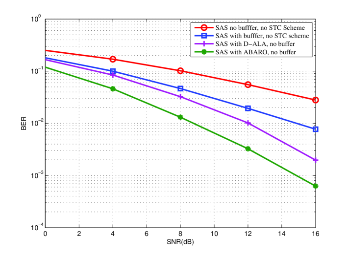
Figure 3: Buffer v.s. No Buffer in SAS

The upper bounds of the D-Alamouti, the proposed ABARO algorithm and the buffer-aided relays in the SAS configurations are shown in Fig. 3. The theoretical PEP result of a standard SAS configuration, which does not employ STC schemes or buffer-aided relays, is shown as the curve contains the largest decoding errors. By comparing the first two BER curves in Fig. 3 we can conclude that by employing buffers at relays, the decoding error upper bound is decreased. In this case, the effect of using buffers at the relays contributes to reducing the PEP performance dramatically. If the STC scheme is employed at the relays, an increase of diversity order is observed in Fig. 3. By comparing the lower BER curves in Fig. 3, we can see that by employing the ABARO algorithm which optimizes the adjustable matrices after each transmission contributes to a lower error probability upper bound. As shown in the previous section, by employing adjustable code matrices and the proposed ABARO algorithm, an improvement of the coding gain is obtained which reduces the error probability.

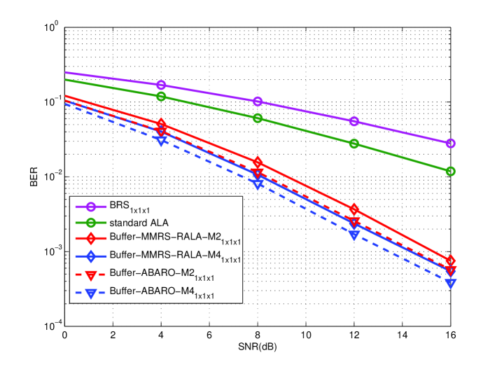
Figure 4: BER Performance vs. $SNR$ for SAS, $1$ Relay

The proposed ABARO algorithm with the Alamouti scheme and an ML receiver in the SAS configuration is evaluated with a single-relay system in Figs. 4 and 5. Different buffer sizes are considered at the relay node. A static channel is employed during the simulation and the corresponding period in which the channel is static is equal to one symbol. The BER results of the cooperative system with the best relay selection (BRS) algorithm in [9] and the max-max relay selection (MMRS) protocols in [16] are shown in both figures. The BER performance of using standard Alamouti scheme at the relays is given as well. No STC schemes are used in Fig. 5 so that the curves achieve a first order diversity. A $2$dB to $3$dB BER improvement in Fig. 5 can be observed by employing MMRS algorithms as compared to the BRS algorithm. According to the simulation results, with the increase of the buffer size at the relay nodes, the improvement in the BER reduces and with the buffer size greater than $6$ the advantages of using buffer-aided relays are not that obvious.

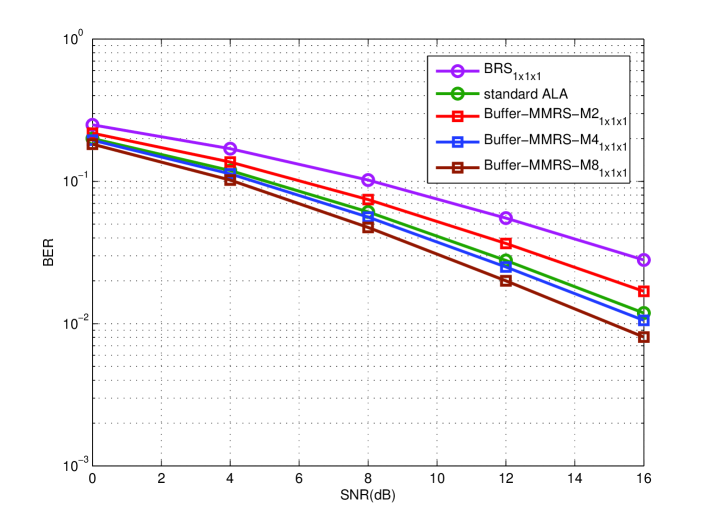
Figure 5: BER Performance vs. $SNR$ for SAS, $1$ Relay

An improvement of diversity order can be observed when using STBC schemes at the relays which is shown in Fig. 6. With the buffer size greater than $4$, the advantage of using STBC schemes at the relays disappears as a function of the diminishing returns in performance. As shown in the simulation results, when the RSTC scheme is considered at the relay node, the BER curve with buffer size of $6$ approaches that with buffer size of $8$ as well. In Fig. 6, the proposed ABARO algorithm is employed in the single-antenna systems with $n_{r}=2$ relay nodes. According to the simulation results in Fig. 6, a $1$dB to $2$dB gain can be achieved by using the proposed ABARO algorithm at the relays as compared to the network using the RSTC scheme at the relay node. The diversity order of the curves associated with the proposed ABARO algorithm is the same as that of using the RSTC scheme at the relay node. Compared to the MMRS algorithm derived in [16] with the same buffer size, the ABARO algorithm achieves a $1$dB to $2$dB improvement.

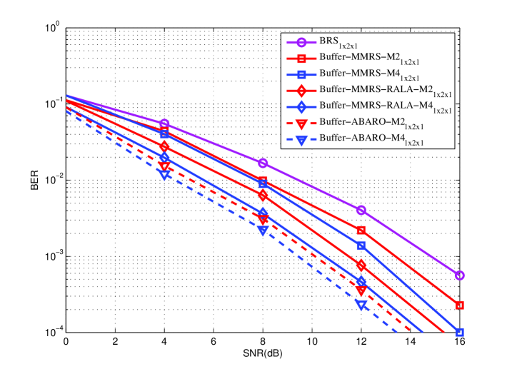
Figure 6: BER Performance vs. $SNR$ for Buffer-Aided Relaying System, $2$ Relays

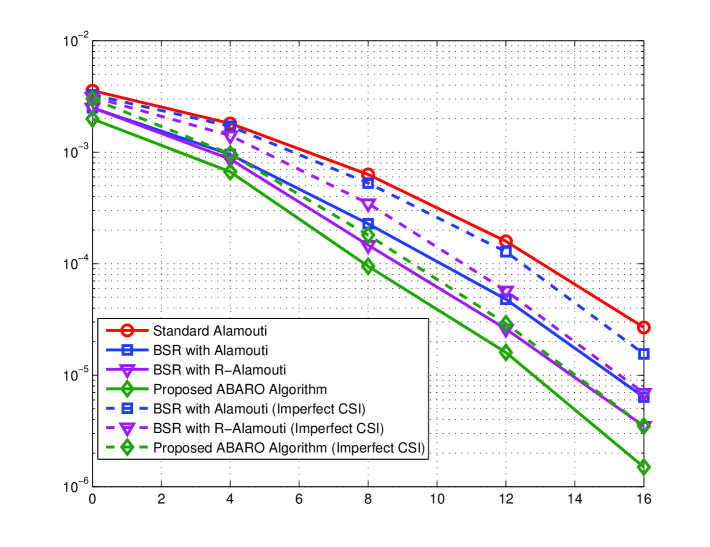
Figure 7: BER Performance vs. $SNR$ for Buffer-Aided Relaying System

The proposed ABARO algorithm with the Alamouti scheme and an ML receiver is evaluated in a MAS configuration with two relays in Fig. 7. It is shown in the figure that the buffer-aided relay selection systems achieve $3$dB to $5$dB gains compared to the previously reported relay systems. When the BSR algorithm is considered at the relay node, an improvement of diversity order is shown in Fig. 7 which leads to significantly improved BER performance. According to the simulation results in Fig. 7, a $1$dB gain can be achieved by using the RSTC scheme at the relays as compared to the network using the standard STC scheme at the relay node. When the proposed ABARO algorithm is employed at the relays, a $2$dB saving for the same BER performance as compared to the standard STC encoded system can be observed. The diversity order of using the proposed ABARO algorithm is the same as that of using the RSTC scheme at the relay node.

The impact of imperfect CSI at the destination node is considered for different schemes as shown in Fig. 7. It is clear that a $2$dB loss of the BER performance is obtained in BRS with Alamouti and R-Alamouti schemes due to the imperfect CSI obtained at the destination node. As we introduce errors in the channel elements in (13)-(16), the accuracy of optimal coding vector is affected. However, according to the simulation result, a $1$dB BER loss is observed in Fig. 7 due to the channel errors. The proposed optimization algorithm is able to maintain the BER performance under the imperfect CSI obtained at the destination node.

VIII Conclusion

We have proposed a buffer-aided space-time coding scheme, relay selection and the ABARO algorithms for cooperative systems with limited feedback using an ML receiver at the destination node to achieve a better BER performance. Simulation results have illustrated the advantage of using the adjustable STC and DSTC schemes in the buffer-aided cooperative systems compared to the BRS algorithms. In addition, the proposed ABARO algorithm can achieve a better performance in terms of lower BER at the destination node as compared to prior art. The ABARO algorithm can be used with different STC schemes and can also be extended to cooperative systems with any number of antennas.

References

- [1] J. N. Laneman and G. W. Wornell, “Cooperative Diversity in Wireless Networks: Efficient Protocols and Outage Behaviour”, IEEE Trans. Inf. Theory, vol. 50, no. 12, pp. 3062-3080, Dec. 2004.
- [2] B. Maham, A. Hjrungnes, G. Abreu, Distributed GABBA Space-Time Codes in Amplify-and-Forward Relay Networks, IEEE Transactions on Wireless Communications, vol.8, Issuse: 4, pp. 2036 - 2045, April 2009.
- [3] S. Yang, J.-C. Belfiore, Optimal Space-Time Codes for the MIMO Amplify-and-Forward Cooperative Channel, IEEE Transactions on Information Theory, vol. 53, Issue: 2, pp. 647-663, Feb. 2007.
- [4] S. Yiu, R. Schober, L. Lampe, Distributed Space-Time Block Coding, IEEE Transactions on Wireless Communications, vol. 54, no. 7, pp. 1195-1206, July 2006.
- [5] J. Abouei, H. Bagheri, A. Khandani, An Efficient Adaptive Distributed Space-Time Coding Scheme for Cooperative Relaying, IEEE Transactions on Wireless Communications, vol. 8, Issue: 10, pp. 4957-4962, October 2009.
- [6] B. Maham, A. Hjrungnes, B. S. Rajan, Quasi-Orthogonal Design and Performance Analysis of Amplify-And-Forward Relay Networks with Multiple-Antennas, IEEE Wireless Communications and Networking Conference (WCNC), 18-21 April 2010.
- [7] P. Clarke and R. C. de Lamare, “Joint Transmit Diversity Optimization and Relay Selection for Multi-relay Cooperative MIMO Systems Using Discrete Stochastic Algorithms”, IEEE Communications Letters, vol. 15, p.p. 1035-1037, Oct. 2011.
- [8] P. Clarke and R. C. de Lamare, “Transmit Diversity and Relay Selection Algorithms for Multi-relay Cooperative MIMO Systems”, IEEE Transactions on Vehicular Technology, vol. 61 , no. 3, March 2012, Page(s): 1084 - 1098.
- [9] A. Bletsas, A. Khisti, D. Reed and A. Lippman, “A simple cooperative diversity method based on network path selection”, IEEE Journal on Selected Areas in Communications, vol. 24 , page(s): 659 - 672, Mar. 2006.
- [10] N. Zlatanov, A. Ikhlef, T. Islam and R. Schober, “Buffer-aided cooperative communications: opportunities and challenges”, IEEE Communications Magazine, vol. 52, pp. 146-153, May 2014.
- [11] N. Zlatanov, R. Schober and P. Popovski, “Throughput and Diversity Gain of Buffer-Aided Relaying”, IEEE GLOBECOM, Dec., 2011.
- [12] N. Zlatanov, R. Schober and P. Popovski, “Buffer-Aided Relaying with Adaptive Link Selection”, IEEE Journal on Selected Areas in Communications, vol. 31, no. 8, Aug. 2013, pp. 1530-1542.
- [13] N. Zlatanov and R. Schober, “Buffer-Aided Relaying with Adaptive Link Selection - Fixed and Mixed Rate Transmission”, IEEE Transactions on Information Theory, vol. 59, no. 5, May 2013, pp. 2816-2840.
- [14] I. Krikidis, T. Charalambous and J. Thompson, “Buffer-Aided Relay Selection for Cooperative Diversity Systems Without Delay Constraints”, IEEE Transactions on Wireless Communications, vol. 11, no. 5, May 2012, pp. 1957-1967.
- [15] A. Ikhlef, J. Kim and R. Schober, “Mimicking Full-Duplex Relaying Using Half-Duplex Relays With Buffers”, IEEE Transactions on Vehicular Technology, vol.61, May 2012, pp. 3025 - 3037.
- [16] A. Ikhlef, D. S. Michalopoulos and R. Schober, “Max-Max Relay Selection for Relays with Buffers”, IEEE Transactions on Wireless Communications, vol.11, January 2012, pp. 1124 - 1135.
- [17] T. Peng and R. C. de Lamare, “Adaptive Buffer-Aided Distributed Space-Time Coding for Cooperative Wireless Networks,” in IEEE Transactions on Communications, vol. 64, no. 5, pp. 1888-1900, May 2016.
- [18] S. Haykin, “Adaptive Filter Theory”, ed., Englewood Cliffs, NJ: Prentice- Hall, 2002.
- [19] B. Sirkeci-Mergen and A. Scaglione, “Randomized Space-Time Coding for Distributed Cooperative Communication”, IEEE Transactions on Signal Processing, vol. 55, no. 10, Oct. 2007.
- [20] T. Peng, R. C. de Lamare and A. Schmeink, “Adaptive Distributed Space-Time Coding Based on Adjustable Code Matrices for Cooperative MIMO Relaying Systems”, IEEE Transactions on Communications, vol. 61, no. 7, July 2013.
- [21] T. Wang, R. C. de Lamare, and P. D. Mitchell, “Low-Complexity Set-Membership Channel Estimation for Cooperative Wireless Sensor Networks,” IEEE Transactions on Vehicular Technology, vol.60, no.6, pp.2594-2607, July 2011.
- [22] S. Zhang, F. Gao, C. Pei, X. He, “Segment Training Based Individual Channel Estimation in One-Way Relay Network with Power Allocation,” IEEE Transactions on Wireless Communications, vol. 12, no. 3, pp. 1300-1309, March 2013.
- [23] B. Hassibi and B. Hochwald, “High-rate codes that are linear in space and time”, IEEE Transactions on Information Theory, vol. 48, Issue 7, pp. 1804-1824, July 2002.
- [24] H. Jafarkhani, Space-Time Coding Theory and Practice, Cambridge University Press, 2005.
- [25] J. Yuan, Z. Chen, B. S. Vucetic, and W. Firmanto, Performance and design of space-time coding in fading channels, IEEE Transactions on Communications, vol. 51, no. 12, p.p. 1991-1996, Dec. 2003.
- [26] N. Nomikos, T. Charalambous, I. Krikidis, D. Skoutas, D. Vouyioukas and M. Johansson, “A Buffer-aided Successive Opportunistic Relay Selection Scheme with Power Adaptation and Inter-Relay Interference Cancellation for Cooperative Diversity Systems”, IEEE International Symposium on Personal Indoor and Mobile Radio Communications, September 2013.
- [27] B. Maham, A. Hjørungnes, “Opportunistic Relaying for MIMO Amplify-and-Forward Cooperative Networks”, Wireless Personal Communications, DOI 10.1007/s11277-011-0499-9, January 2012.
- [28] L. L. Scharf and D. W. Tufts, “Rank reduction for modeling stationary signals,” IEEE Transactions on Acoustics, Speech and Signal Processing, vol. ASSP-35, pp. 350-355, March 1987.
- [29] A. M. Haimovich and Y. Bar-Ness, “An eigenanalysis interference canceler,” IEEE Trans. on Signal Processing, vol. 39, pp. 76-84, Jan. 1991.
- [30] D. A. Pados and S. N. Batalama ”Joint space-time auxiliary vector filtering for DS/CDMA systems with antenna arrays” IEEE Transactions on Communications, vol. 47, no. 9, pp. 1406 - 1415, 1999.
- [31] J. S. Goldstein, I. S. Reed and L. L. Scharf ”A multistage representation of the Wiener filter based on orthogonal projections” IEEE Transactions on Information Theory, vol. 44, no. 7, 1998.
- [32] Y. Hua, M. Nikpour and P. Stoica, ”Optimal reduced rank estimation and filtering,” IEEE Transactions on Signal Processing, pp. 457-469, Vol. 49, No. 3, March 2001.
- [33] M. L. Honig and J. S. Goldstein, “Adaptive reduced-rank interference suppression based on the multistage Wiener filter,” IEEE Transactions on Communications, vol. 50, no. 6, June 2002.
- [34] E. L. Santos and M. D. Zoltowski, “On Low Rank MVDR Beamforming using the Conjugate Gradient Algorithm”, Proc. IEEE International Conference on Acoustics, Speech and Signal Processing, 2004.
- [35] Q. Haoli and S.N. Batalama, “Data record-based criteria for the selection of an auxiliary vector estimator of the MMSE/MVDR filter”, IEEE Transactions on Communications, vol. 51, no. 10, Oct. 2003, pp. 1700 - 1708.
- [36] R. C. de Lamare and R. Sampaio-Neto, “Reduced-Rank Adaptive Filtering Based on Joint Iterative Optimization of Adaptive Filters”, IEEE Signal Processing Letters, Vol. 14, no. 12, December 2007.
- [37] Z. Xu and M.K. Tsatsanis, “Blind adaptive algorithms for minimum variance CDMA receivers,” IEEE Trans. Communications, vol. 49, No. 1, January 2001.
- [38] R. C. de Lamare and R. Sampaio-Neto, “Low-Complexity Variable Step-Size Mechanisms for Stochastic Gradient Algorithms in Minimum Variance CDMA Receivers”, IEEE Trans. Signal Processing, vol. 54, pp. 2302 - 2317, June 2006.
- [39] C. Xu, G. Feng and K. S. Kwak, “A Modified Constrained Constant Modulus Approach to Blind Adaptive Multiuser Detection,” IEEE Trans. Communications, vol. 49, No. 9, 2001.
- [40] Z. Xu and P. Liu, “Code-Constrained Blind Detection of CDMA Signals in Multipath Channels,” IEEE Sig. Proc. Letters, vol. 9, No. 12, December 2002.
- [41] R. C. de Lamare and R. Sampaio Neto, ”Blind Adaptive Code-Constrained Constant Modulus Algorithms for CDMA Interference Suppression in Multipath Channels”, IEEE Communications Letters, vol 9. no. 4, April, 2005.
- [42] L. Landau, R. C. de Lamare and M. Haardt, “Robust adaptive beamforming algorithms using the constrained constant modulus criterion,” IET Signal Processing, vol.8, no.5, pp.447-457, July 2014.
- [43] R. C. de Lamare, “Adaptive Reduced-Rank LCMV Beamforming Algorithms Based on Joint Iterative Optimisation of Filters”, Electronics Letters, vol. 44, no. 9, 2008.
- [44] R. C. de Lamare and R. Sampaio-Neto, “Adaptive Reduced-Rank Processing Based on Joint and Iterative Interpolation, Decimation and Filtering”, IEEE Transactions on Signal Processing, vol. 57, no. 7, July 2009, pp. 2503 - 2514.
- [45] R. C. de Lamare and Raimundo Sampaio-Neto, “Reduced-rank Interference Suppression for DS-CDMA based on Interpolated FIR Filters”, IEEE Communications Letters, vol. 9, no. 3, March 2005.
- [46] R. C. de Lamare and R. Sampaio-Neto, “Adaptive Reduced-Rank MMSE Filtering with Interpolated FIR Filters and Adaptive Interpolators”, IEEE Signal Processing Letters, vol. 12, no. 3, March, 2005.
- [47] R. C. de Lamare and R. Sampaio-Neto, “Adaptive Interference Suppression for DS-CDMA Systems based on Interpolated FIR Filters with Adaptive Interpolators in Multipath Channels”, IEEE Trans. Vehicular Technology, Vol. 56, no. 6, September 2007.
- [48] R. C. de Lamare, “Adaptive Reduced-Rank LCMV Beamforming Algorithms Based on Joint Iterative Optimisation of Filters,” Electronics Letters, 2008.
- [49] R. C. de Lamare and R. Sampaio-Neto, “Reduced-rank adaptive filtering based on joint iterative optimization of adaptive filters”, IEEE Signal Process. Lett., vol. 14, no. 12, pp. 980-983, Dec. 2007.
- [50] R. C. de Lamare, M. Haardt, and R. Sampaio-Neto, “Blind Adaptive Constrained Reduced-Rank Parameter Estimation based on Constant Modulus Design for CDMA Interference Suppression”, IEEE Transactions on Signal Processing, June 2008.
- [51] M. Yukawa, R. C. de Lamare and R. Sampaio-Neto, “Efficient Acoustic Echo Cancellation With Reduced-Rank Adaptive Filtering Based on Selective Decimation and Adaptive Interpolation,” IEEE Transactions on Audio, Speech, and Language Processing, vol.16, no. 4, pp. 696-710, May 2008.
- [52] R. C. de Lamare and R. Sampaio-Neto, “Reduced-rank space-time adaptive interference suppression with joint iterative least squares algorithms for spread-spectrum systems,” IEEE Trans. Vehi. Technol., vol. 59, no. 3, pp. 1217-1228, Mar. 2010.
- [53] R. C. de Lamare and R. Sampaio-Neto, “Adaptive reduced-rank equalization algorithms based on alternating optimization design techniques for MIMO systems,” IEEE Trans. Vehi. Technol., vol. 60, no. 6, pp. 2482-2494, Jul. 2011.
- [54] R. C. de Lamare, L. Wang, and R. Fa, “Adaptive reduced-rank LCMV beamforming algorithms based on joint iterative optimization of filters: Design and analysis,” Signal Processing, vol. 90, no. 2, pp. 640-652, Feb. 2010.
- [55] R. Fa, R. C. de Lamare, and L. Wang, “Reduced-Rank STAP Schemes for Airborne Radar Based on Switched Joint Interpolation, Decimation and Filtering Algorithm,” IEEE Transactions on Signal Processing, vol.58, no.8, Aug. 2010, pp.4182-4194.
- [56] L. Wang and R. C. de Lamare, ”Low-Complexity Adaptive Step Size Constrained Constant Modulus SG Algorithms for Blind Adaptive Beamforming”, Signal Processing, vol. 89, no. 12, December 2009, pp. 2503-2513.
- [57] L. Wang and R. C. de Lamare, “Adaptive Constrained Constant Modulus Algorithm Based on Auxiliary Vector Filtering for Beamforming,” IEEE Transactions on Signal Processing, vol. 58, no. 10, pp. 5408-5413, Oct. 2010.
- [58] L. Wang, R. C. de Lamare, M. Yukawa, ”Adaptive Reduced-Rank Constrained Constant Modulus Algorithms Based on Joint Iterative Optimization of Filters for Beamforming,” IEEE Transactions on Signal Processing, vol.58, no.6, June 2010, pp.2983-2997.
- [59] L. Wang, R. C. de Lamare and M. Yukawa, “Adaptive reduced-rank constrained constant modulus algorithms based on joint iterative optimization of filters for beamforming”, IEEE Transactions on Signal Processing, vol.58, no. 6, pp. 2983-2997, June 2010.
- [60] L. Wang and R. C. de Lamare, “Adaptive constrained constant modulus algorithm based on auxiliary vector filtering for beamforming”, IEEE Transactions on Signal Processing, vol. 58, no. 10, pp. 5408-5413, October 2010.
- [61] R. Fa and R. C. de Lamare, “Reduced-Rank STAP Algorithms using Joint Iterative Optimization of Filters,” IEEE Transactions on Aerospace and Electronic Systems, vol.47, no.3, pp.1668-1684, July 2011.
- [62] Z. Yang, R. C. de Lamare and X. Li, “L1-Regularized STAP Algorithms With a Generalized Sidelobe Canceler Architecture for Airborne Radar,” IEEE Transactions on Signal Processing, vol.60, no.2, pp.674-686, Feb. 2012.
- [63] Z. Yang, R. C. de Lamare and X. Li, “Sparsity-aware space-time adaptive processing algorithms with L1-norm regularisation for airborne radar,” IET signal processing, vol. 6, no. 5, pp. 413-423, 2012.
- [64] Neto, F.G.A.; Nascimento, V.H.; Zakharov, Y.V.; de Lamare, R.C., “Adaptive re-weighting homotopy for sparse beamforming,” in Signal Processing Conference (EUSIPCO), 2014 Proceedings of the 22nd European , vol., no., pp.1287-1291, 1-5 Sept. 2014
- [65] Almeida Neto, F.G.; de Lamare, R.C.; Nascimento, V.H.; Zakharov, Y.V.,“Adaptive reweighting homotopy algorithms applied to beamforming,” IEEE Transactions on Aerospace and Electronic Systems, vol.51, no.3, pp.1902-1915, July 2015.
- [66] L. Wang, R. C. de Lamare and M. Haardt, “Direction finding algorithms based on joint iterative subspace optimization,” IEEE Transactions on Aerospace and Electronic Systems, vol.50, no.4, pp.2541-2553, October 2014.
- [67] S. D. Somasundaram, N. H. Parsons, P. Li and R. C. de Lamare, “Reduced-dimension robust capon beamforming using Krylov-subspace techniques,” IEEE Transactions on Aerospace and Electronic Systems, vol.51, no.1, pp.270-289, January 2015.
- [68] S. Xu and R.C de Lamare, , Distributed conjugate gradient strategies for distributed estimation over sensor networks, Sensor Signal Processing for Defense SSPD, September 2012.
- [69] S. Xu, R. C. de Lamare, H. V. Poor, “Distributed Estimation Over Sensor Networks Based on Distributed Conjugate Gradient Strategies”, IET Signal Processing, 2016 (to appear).
- [70] S. Xu, R. C. de Lamare and H. V. Poor, Distributed Compressed Estimation Based on Compressive Sensing, IEEE Signal Processing letters, vol. 22, no. 9, September 2014.
- [71] S. Xu, R. C. de Lamare and H. V. Poor, “Distributed reduced-rank estimation based on joint iterative optimization in sensor networks,” in Proceedings of the 22nd European Signal Processing Conference (EUSIPCO), pp.2360-2364, 1-5, Sept. 2014
- [72] S. Xu, R. C. de Lamare and H. V. Poor, “Adaptive link selection strategies for distributed estimation in diffusion wireless networks,” in Proc. IEEE International Conference onAcoustics, Speech and Signal Processing (ICASSP), , vol., no., pp.5402-5405, 26-31 May 2013.
- [73] S. Xu, R. C. de Lamare and H. V. Poor, “Dynamic topology adaptation for distributed estimation in smart grids,” in Computational Advances in Multi-Sensor Adaptive Processing (CAMSAP), 2013 IEEE 5th International Workshop on , vol., no., pp.420-423, 15-18 Dec. 2013.
- [74] S. Xu, R. C. de Lamare and H. V. Poor, “Adaptive Link Selection Algorithms for Distributed Estimation”, EURASIP Journal on Advances in Signal Processing, 2015.
- [75] N. Song, R. C. de Lamare, M. Haardt, and M. Wolf, “Adaptive Widely Linear Reduced-Rank Interference Suppression based on the Multi-Stage Wiener Filter,” IEEE Transactions on Signal Processing, vol. 60, no. 8, 2012.
- [76] N. Song, W. U. Alokozai, R. C. de Lamare and M. Haardt, “Adaptive Widely Linear Reduced-Rank Beamforming Based on Joint Iterative Optimization,” IEEE Signal Processing Letters, vol.21, no.3, pp. 265-269, March 2014.
- [77] R.C. de Lamare, R. Sampaio-Neto and M. Haardt, ”Blind Adaptive Constrained Constant-Modulus Reduced-Rank Interference Suppression Algorithms Based on Interpolation and Switched Decimation,” IEEE Trans. on Signal Processing, vol.59, no.2, pp.681-695, Feb. 2011.
- [78] Y. Cai, R. C. de Lamare, “Adaptive Linear Minimum BER Reduced-Rank Interference Suppression Algorithms Based on Joint and Iterative Optimization of Filters,” IEEE Communications Letters, vol.17, no.4, pp.633-636, April 2013.
- [79] R. C. de Lamare and R. Sampaio-Neto, “Sparsity-Aware Adaptive Algorithms Based on Alternating Optimization and Shrinkage,” IEEE Signal Processing Letters, vol.21, no.2, pp.225,229, Feb. 2014.
- [80] L. Qiu, Y. Cai, R. C. de Lamare and M. Zhao, “Reduced-Rank DOA Estimation Algorithms Based on Alternating Low-Rank Decomposition,” in IEEE Signal Processing Letters, vol. 23, no. 5, pp. 565-569, May 2016.
- [81] R. C. de Lamare, “Massive MIMO Systems: Signal Processing Challenges and Future Trends”, Radio Science Bulletin, December 2013.
- [82] W. Zhang, H. Ren, C. Pan, M. Chen, R. C. de Lamare, B. Du and J. Dai, “Large-Scale Antenna Systems With UL/DL Hardware Mismatch: Achievable Rates Analysis and Calibration”, IEEE Trans. Commun., vol.63, no.4, pp. 1216-1229, April 2015.
- [83] M. Costa, ”Writing on dirty paper,” IEEE Trans. Inform. Theory, vol. 29, no. 3, pp. 439-441, May 1983.
- [84] R. C. de Lamare and A. Alcaim, ”Strategies to improve the performance of very low bit rate speech coders and application to a 1.2 kb/s codec” IEE Proceedings- Vision, image and signal processing, vol. 152, no. 1, February, 2005.
- [85] P. Clarke and R. C. de Lamare, ”Joint Transmit Diversity Optimization and Relay Selection for Multi-Relay Cooperative MIMO Systems Using Discrete Stochastic Algorithms,” IEEE Communications Letters, vol.15, no.10, pp.1035-1037, October 2011.
- [86] P. Clarke and R. C. de Lamare, ”Transmit Diversity and Relay Selection Algorithms for Multirelay Cooperative MIMO Systems” IEEE Transactions on Vehicular Technology, vol.61, no. 3, pp. 1084-1098, March 2012.
- [87] T. Peng, R. C. de Lamare and A. Schmeink, “Adaptive Distributed Space-Time Coding Based on Adjustable Code Matrices for Cooperative MIMO Relaying Systems,” IEEE Transactions on Communications, vol. 61, no. 7, pp. 2692-2703, July 2013.
- [88] T. Peng and R. C. de Lamare, “Adaptive Buffer-Aided Distributed Space-Time Coding for Cooperative Wireless Networks,” IEEE Transactions on Communications, vol. 64, no. 5, pp. 1888-1900, May 2016.
- [89] Y. Cai, R. C. de Lamare, and R. Fa, “Switched Interleaving Techniques with Limited Feedback for Interference Mitigation in DS-CDMA Systems,” IEEE Transactions on Communications, vol.59, no.7, pp.1946-1956, July 2011.
- [90] Y. Cai, R. C. de Lamare, D. Le Ruyet, “Transmit Processing Techniques Based on Switched Interleaving and Limited Feedback for Interference Mitigation in Multiantenna MC-CDMA Systems,” IEEE Transactions on Vehicular Technology, vol.60, no.4, pp.1559-1570, May 2011.
- [91] T. Wang, R. C. de Lamare, and P. D. Mitchell, “Low-Complexity Set-Membership Channel Estimation for Cooperative Wireless Sensor Networks,” IEEE Transactions on Vehicular Technology, vol.60, no.6, pp.2594-2607, July 2011.
- [92] T. Wang, R. C. de Lamare and A. Schmeink, ”Joint linear receiver design and power allocation using alternating optimization algorithms for wireless sensor networks,” IEEE Trans. on Vehi. Tech., vol. 61, pp. 4129-4141, 2012.
- [93] R. C. de Lamare, “Joint iterative power allocation and linear interference suppression algorithms for cooperative DS-CDMA networks”, IET Communications, vol. 6, no. 13 , 2012, pp. 1930-1942.
- [94] T. Peng, R. C. de Lamare and A. Schmeink, “Adaptive Distributed Space-Time Coding Based on Adjustable Code Matrices for Cooperative MIMO Relaying Systems”, IEEE Transactions on Communications, vol. 61, no. 7, July 2013.
- [95] K. Zu, R. C. de Lamare, “Low-Complexity Lattice Reduction-Aided Regularized Block Diagonalization for MU-MIMO Systems”, IEEE. Communications Letters, Vol. 16, No. 6, June 2012, pp. 925-928.
- [96] K. Zu, R. C. de Lamare, “Low-Complexity Lattice Reduction-Aided Regularized Block Diagonalization for MU-MIMO Systems”, IEEE. Communications Letters, Vol. 16, No. 6, June 2012.
- [97] K. Zu, R. C. de Lamare and M. Haart, “Generalized design of low-complexity block diagonalization type precoding algorithms for multiuser MIMO systems”, IEEE Trans. Communications, 2013.
- [98] M. Tomlinson, ”New automatic equaliser employing modulo arithmetic,” Electronic Letters, vol. 7, Mar. 1971.
- [99] C. T. Healy and R. C. de Lamare, “Decoder-optimised progressive edge growth algorithms for the design of LDPC codes with low error floors”, IEEE Communications Letters, vol. 16, no. 6, June 2012, pp. 889-892.
- [100] A. G. D. Uchoa, C. T. Healy, R. C. de Lamare, R. D. Souza, “LDPC codes based on progressive edge growth techniques for block fading channels”, Proc. 8th International Symposium on Wireless Communication Systems (ISWCS), 2011, pp. 392-396.
- [101] A. G. D. Uchoa, C. T. Healy, R. C. de Lamare, R. D. Souza, “Generalised Quasi-Cyclic LDPC codes based on progressive edge growth techniques for block fading channels”, Proc. International Symposium Wireless Communication Systems (ISWCS), 2012, pp. 974-978.
- [102] A. G. D. Uchoa, C. T. Healy, R. C. de Lamare, R. D. Souza, “Design of LDPC Codes Based on Progressive Edge Growth Techniques for Block Fading Channels”, IEEE Communications Letters, vol. 15, no. 11, November 2011, pp. 1221-1223.
- [103] C. T. Healy and R. C. de Lamare, “Design of LDPC Codes Based on Multipath EMD Strategies for Progressive Edge Growth”, IEEE Transactions on Communications, 2016.
- [104] H. Harashima and H. Miyakawa, ”Matched-transmission technique for channels with intersymbol interference,” IEEE Trans. Commun., vol. 20, Aug. 1972.
- [105] K. Zu, R. C. de Lamare and M. Haardt, “Multi-branch tomlinson-harashima precoding for single-user MIMO systems,” in Smart Antennas (WSA), 2012 International ITG Workshop on , vol., no., pp.36-40, 7-8 March 2012.
- [106] K. Zu, R. C. de Lamare and M. Haardt, “Multi-Branch Tomlinson-Harashima Precoding Design for MU-MIMO Systems: Theory and Algorithms,” IEEE Transactions on Communications, vol.62, no.3, pp.939,951, March 2014.
- [107] L. Zhang, Y. Cai, R. C. de Lamare and M. Zhao, “Robust Multibranch Tomlinson-Harashima Precoding Design in Amplify-and-Forward MIMO Relay Systems,” IEEE Transactions on Communications, vol.62, no.10, pp. 3476-3490, Oct. 2014.
- [108] Y. Cai, R. C. de Lamare, L. L. Yang and M. Zhao, “Robust MMSE Precoding Based on Switched Relaying and Side Information for Multiuser MIMO Relay Systems,” IEEE Transactions on Vehicular Technology, vol. 64, no. 12, pp. 5677-5687, Dec. 2015.
- [109] B. Hochwald, C. Peel and A. Swindlehurst, ”A vector-perturbation technique for near capacity multiantenna multiuser communication - Part II: Perturbation,” IEEE Trans. Commun., vol. 53, no. 3, Mar. 2005.
- [110] C. B. Chae, S. Shim and R. W. Heath, ”Block diagonalized vector perturbation for multiuser MIMO systems,” IEEE Trans. Wireless Commun., vol. 7, no. 11, pp. 4051 - 4057, Nov. 2008.
- [111] R. C. de Lamare, R. Sampaio-Neto, “Adaptive MBER decision feedback multiuser receivers in frequency selective fading channels”, IEEE Communications Letters, vol. 7, no. 2, Feb. 2003, pp. 73 - 75.
- [112] A. Rontogiannis, V. Kekatos, and K. Berberidis,” A Square-Root Adaptive V-BLAST Algorithm for Fast Time-Varying MIMO Channels,” IEEE Signal Processing Letters, Vol. 13, No. 5, pp. 265-268, May 2006.
- [113] R. C. de Lamare, R. Sampaio-Neto, A. Hjorungnes, “Joint iterative interference cancellation and parameter estimation for CDMA systems”, IEEE Communications Letters, vol. 11, no. 12, December 2007, pp. 916 - 918.
- [114] Y. Cai and R. C. de Lamare, ”Adaptive Space-Time Decision Feedback Detectors with Multiple Feedback Cancellation”, IEEE Transactions on Vehicular Technology, vol. 58, no. 8, October 2009, pp. 4129 - 4140.
- [115] J. W. Choi, A. C. Singer, J Lee, N. I. Cho, “Improved linear soft-input soft-output detection via soft feedback successive interference cancellation,” IEEE Trans. Commun., vol.58, no.3, pp.986-996, March 2010.
- [116] R. C. de Lamare and R. Sampaio-Neto, “Blind adaptive MIMO receivers for space-time block-coded DS-CDMA systems in multipath channels using the constant modulus criterion,” IEEE Transactions on Communications, vol.58, no.1, pp.21-27, January 2010.
- [117] R. Fa, R. C. de Lamare, “Multi-Branch Successive Interference Cancellation for MIMO Spatial Multiplexing Systems”, IET Communications, vol. 5, no. 4, pp. 484 - 494, March 2011.
- [118] R.C. de Lamare and R. Sampaio-Neto, “Adaptive reduced-rank equalization algorithms based on alternating optimization design techniques for MIMO systems,” IEEE Trans. Veh. Technol., vol. 60, no. 6, pp. 2482-2494, July 2011.
- [119] P. Li, R. C. de Lamare and R. Fa, “Multiple Feedback Successive Interference Cancellation Detection for Multiuser MIMO Systems,” IEEE Transactions on Wireless Communications, vol. 10, no. 8, pp. 2434 - 2439, August 2011.
- [120] R.C. de Lamare, R. Sampaio-Neto, “Minimum mean-squared error iterative successive parallel arbitrated decision feedback detectors for DS-CDMA systems,” IEEE Trans. Commun., vol. 56, no. 5, May 2008, pp. 778-789.
- [121] R.C. de Lamare, R. Sampaio-Neto, “Minimum mean-squared error iterative successive parallel arbitrated decision feedback detectors for DS-CDMA systems,” IEEE Trans. Commun., vol. 56, no. 5, May 2008.
- [122] R.C. de Lamare and R. Sampaio-Neto, “Adaptive reduced-rank equalization algorithms based on alternating optimization design techniques for MIMO systems,” IEEE Trans. Veh. Technol., vol. 60, no. 6, pp. 2482-2494, July 2011.
- [123] P. Li, R. C. de Lamare and J. Liu, “Adaptive Decision Feedback Detection with Parallel Interference Cancellation and Constellation Constraints for Multiuser MIMO systems”, IET Communications, vol.7, 2012, pp. 538-547.
- [124] J. Liu, R. C. de Lamare, “Low-Latency Reweighted Belief Propagation Decoding for LDPC Codes,” IEEE Communications Letters, vol. 16, no. 10, pp. 1660-1663, October 2012.
- [125] C. T. Healy and R. C. de Lamare, “Design of LDPC Codes Based on Multipath EMD Strategies for Progressive Edge Growth,” in IEEE Transactions on Communications, vol. 64, no. 8, pp. 3208-3219, Aug. 2016.
- [126] P. Li and R. C. de Lamare, Distributed Iterative Detection With Reduced Message Passing for Networked MIMO Cellular Systems, IEEE Transactions on Vehicular Technology, vol.63, no.6, pp. 2947-2954, July 2014.
- [127] A. G. D. Uchoa, C. T. Healy and R. C. de Lamare, “Iterative Detection and Decoding Algorithms For MIMO Systems in Block-Fading Channels Using LDPC Codes,” IEEE Transactions on Vehicular Technology, 2015.
- [128] R. C. de Lamare, “Adaptive and Iterative Multi-Branch MMSE Decision Feedback Detection Algorithms for Multi-Antenna Systems”, IEEE Trans. Wireless Commun., vol. 14, no. 10, October 2013.
- [129] Y. Cai, R. C. de Lamare, B. Champagne, B. Qin and M. Zhao, ”Adaptive Reduced-Rank Receive Processing Based on Minimum Symbol-Error-Rate Criterion for Large-Scale Multiple-Antenna Systems,” in IEEE Transactions on Communications, vol. 63, no. 11, pp. 4185-4201, Nov. 2015.