Quantum dynamics of a macroscopic magnet operating as environment of a mechanical oscillator

Abstract

We study the dynamics of a bipartite quantum system in a way such that its formal description keeps holding even if one of its parts becomes macroscopic: the problem is related with the analysis of the quantum-to-classical crossover, but our approach implies that the whole system stays genuinely quantum. Aim of the work is to understand 1) if, 2) to what extent, and possibly 3) how, the evolution of a macroscopic environment testifies to the coupling with its microscopic quantum companion. To this purpose we consider a magnetic environment made of a large number of spin-$\frac{1}{2}$ particles, coupled with a quantum mechanical oscillator, possibly in the presence of an external magnetic field. We take the value of the total environmental-spin $S$ constant and large, which allows us to consider the environment as one single macroscopic system, and further deal with the hurdles of the spin-algebra via approximations that are valid in the large-$S$ limit. We find an insightful expression for the propagator of the whole system, where we identify an effective ”back-action” term, i.e. an operator acting on the magnetic environment only, and yet missing in the absence of the quantum principal system. This operator emerges as a time-dependent magnetic anisotropy whose character, whether uniaxial or planar, also depends on the detuning between the level-splitting in the spectrum of the free magnetic system, induced by the possible presence of the external field, and the frequency of the oscillator. The time-dependence of the anisotropy is analysed, and its effects on the dynamics of the magnet, as well as its relation with the entangling evolution of the overall system, are discussed.

Introduction

For almost the whole last century the problem of how a principal quantum system ($\Gamma$) behaves when interacting with a macroscopic environment ($\Xi$) has been considered assuming the latter to be a classical system. If this is the case, a quantum analysis of how the two subsystems evolve due to their reciprocal interaction is hindered, which is quite a severe limitation since macroscopic environments are the tools by which we ultimately extract information about, or exercise control upon, any microscopic quantum system (Schlosshauer, 2007; Rivas and Huelga, 2012; Breuer and Petruccione, 2002; Paladino et al., 2002). In particular, the effects of the presence of $\Gamma$ on the way $\Xi$ evolves (often referred to as ”back-action” in the literature) have no place in the description, and entanglement between the twos is neglected.

Recently, however, hybrid schemes in which micro- and macroscopic systems coexist in a quantum device have been considered in different frameworks, from the analysis of foundational issues via optomechanical setups, to quantum thermodynamics or nanoelectronics (Lo Franco et al., 2013; Xu et al., 2013; Matsumoto, 2015; Kippenberg and Vahala, 2008; Verhagen et al., 2012). In fact, it is not completely clear why one should renounce a quantum description of a macroscopic system: after all, this is nothing but a system made of many quantum particles that, for one reason or another, can be described regardless of its internal structure as if it were a single object with its own, effective, Hilbert space. The exemplary case of such situation is when $\Xi$ is made by a large number $N$ of spin-$\frac{1}{2}$ particles and is such that its total spin $S$ is a conserved quantity: no matter how large $N$ is, the corresponding magnetic environment behaves, in general, as a quantum system: this is clearly seen if its total spin equals, say, $S=1/2$ or $S=1$. On the other hand, for $S\propto N\to\infty$ a classical-like dynamics is expected Lieb (1973), while large-$S$ approximations are ideal tools for studying macroscopic, and yet quantum, magnetic systems. In general, models that are hybrid in the sense explained above must be studied with the toolkit of open quantum systems enriched by specific accessories for dealing with the macroscopicity of some of their elements.

With this in mind, we here consider a magnetic environment $\Xi$, made by a large number $N$ of spin-$\frac{1}{2}$ particles, featuring a global symmetry that guarantees the total spin $S$ to be a constant of motion. As far as $S$ is finite, such magnet is the prototype of a system that exhibits a distinct quantum behaviour despite being macroscopic ($N\gg 1$). The microscopic companion of the magnet is assumed to be a quantum mechanical oscillator $\Gamma$, with which $\Xi$ exchanges energy according to a model-Hamiltonian that goes beyond the pure-dephasing interaction (Palma et al., 1996; Cucchietti et al., 2010).

We address the time evolution of the composite system $\Gamma+\Xi$ by a large-$S$ approximation that represents the macroscopicity of $\Xi$, since $N\geq 2S$ holds, without totally wiping out its quantum character, since $S$ is finite. Moreover, such an approximation allows us to deal with the complications due to the involved algebra of the spins; in fact, making use of recent results Fernando Casas (2012) on the factorization of operatorial exponentials, and the Zassenhaus formulaZassenhaus (1939); Fernando Casas (2012), we obtain a factorized expression for the propagator of the composite system and find that, due to the coupling between $\Gamma$ and $\Xi$, a specific term appears, effectively representing the back-action of the principal system on its environment. Indeed, the factorization of the propagator allows us to define a free effective Hamiltonian which includes the back-action term in the form of a time-dependent magnetic anisotropy, whose intensity and character (axial or planar) vary, to represent the non-entangling component of the dynamics due to the interaction with the underlying quantum oscillator.

The work is structured as follows: in Sec. I we define the magnetic environment $\Xi$ and briefly discuss the relation between the large-$S$ condition and macroscopicity. The principal system $\Gamma$ enters the scene in Sec. II, where the Hamiltonian, containing an interaction of Tavis-Cummings form Tavis and Cummings (1968), is introduced. The propagator is evaluated in Sec.III, making use of the Zassenhaus expression in the large-$S$ approximation. Results are presented in Secs. IV-V, and conclusions drawn in Sec. VI.

I The magnetic environment

Let us consider a magnetic system $\Xi$ made of $N$ spin-$\frac{1}{2}$ particles, each described by its Pauli matrices $(\hat{\sigma}_{i}^{x},\hat{\sigma}_{i}^{y},\hat{\sigma}_{i}^{z})\equiv\hat{\boldsymbol{\sigma}}_{i}$. As we will always understand $\hslash$ finite, we can hereafter set $\hslash=1$. Be $\hat{\boldsymbol{S}}\equiv\frac{1}{2}\sum_{i}^{N}\hat{\boldsymbol{\sigma}}_{i}$ the total spin of $\Xi$ and $|\hat{\boldsymbol{S}}|^{2}\equiv(\hat{S}^{x})^{2}+(\hat{S}^{y})^{2}+(\hat{S}^{z})^{2}=S(S+1)$, with $S$ ranging from $0$ to $N/2$ if $N$ is even (from $1/2$ to $N/2$ if $N$ is odd). When $|\hat{\boldsymbol{S}}|^{2}$ commutes with the propagator, the value $S$ stays constant and $\Xi$ can be seen as one single physical system described by the spin operators closed under the $su(2)$ commutation relations $[\hat{S}^{\alpha},\hat{S}^{\beta}]=i\varepsilon_{\alpha\beta\gamma}\hat{S}^{\gamma}$, with $\alpha(\beta,\gamma)=x,y,z$. Notice that taking $|\hat{\boldsymbol{S}}|^{2}$ conserved implies assuming that a global symmetry exists in the Hamiltonian acting on $\Xi$, where ”global” means that its generators, amongst which $|\hat{\boldsymbol{S}}|^{2}$ itself, have the same, non-trivial, action on the Hilbert space of any of the $\Xi$-components. One such symmetry characterizes, for instance, a system made by $N$ spin-$\frac{1}{2}$ particles, possibly distributed on the sites of a ring (see Fig. 1), which are either independent or coupled amongst themselves via a homogeneous, isotropic (or Ising) nearest-neighbour interaction, $j\sum_{i}\hat{\boldsymbol{\sigma}}_{i}\cdot\hat{\boldsymbol{\sigma}}_{i+1}$ (or $j\sum_{i}\hat{\sigma}^{\alpha}_{i}\hat{\sigma}^{\alpha}_{i+1}$).

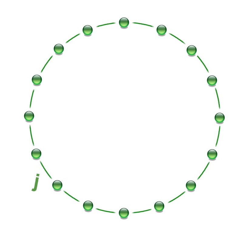
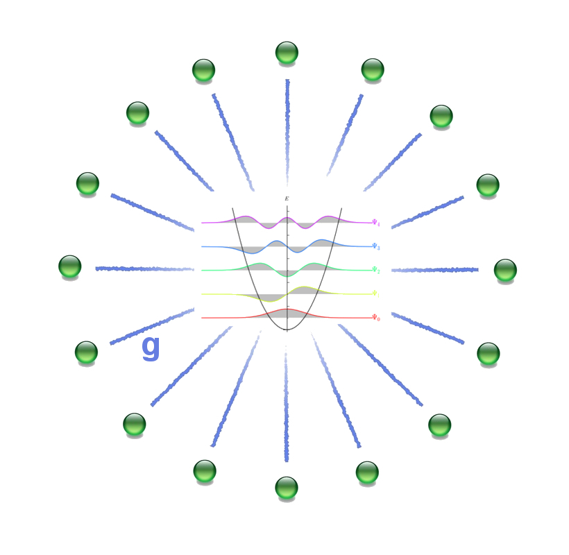
Figure 1: Graphical representation of a magnetic system made of distinguishable particles, with equal spin, distributed on a ring-shaped lattice (referred to as a ”spin-ring” in the text). In panel (a) the system is isolated and its components interact with each other; in panel (b) the system is coupled with a quantum mechanical oscillator and its components are independent from each other.

Once the total spin is guaranteed a constant value $S$, one can consider that $S\to\infty$ is a necessary condition for spin systems to behave classically. In fact, without entering into the detailed formalism that allows one to consistently describe the quantum-to-classical crossover of a magnetic system Lieb (1973); Yaffe (1982), this can be naively understood by the following argument: defining the normalized spin operator $\hat{\boldsymbol{s}}{\equiv}\hat{\boldsymbol{S}}/S$, it is $[\hat{\boldsymbol{s}}^{\alpha},\hat{\boldsymbol{s}}^{\beta}]=i\varepsilon_{\alpha\beta\gamma}\hat{\boldsymbol{s}}^{\gamma}/S$, which implies that $\hat{\boldsymbol{s}}$ becomes a classical vector in the $S\rightarrow\infty$ limit. In Sec. III.1 we will show how to introduce a large-$S$ approximation, essentially based on the above argument.

II The quantum partner

The ”spin-ring” introduced in the previous Section, see Fig. 1(a), is now identified as the magnetic environment $\Xi$ of a quantum mechanical oscillator $\Gamma$, see Fig. 1(b). We choose the Hamiltonian of the overall system of the form

$$\hat{H}=\omega\hat{a}^{\dagger}\hat{a}+\frac{h}{2}\sum_{i}^{N}\hat{\sigma}_{i}^{z}+\frac{1}{2}\sum_{i}^{N}g_{i}(\hat{a}\hat{\sigma}_{i}^{+}+\hat{a}^{\dagger}\hat{\sigma}_{i}^{-})~{},$$ (1)

where $h$ is an external field defining the $z$ axis, and $\hat{\sigma}^{\pm}_{i}\equiv\hat{\sigma}_{i}^{x}\pm i\hat{\sigma}_{i}^{y}$; the different $g_{i}$ are the couplings between each spin of the ring and the oscillator. Being $\hbar=1$, for the bosonic operators describing the principal system it holds $[\hat{a},\hat{a}^{\dagger}]=\hat{\mathbb{I}}$.

In order for the model (1) to describe a system whose environment can be made macroscopic, one needs guaranteeing the existence of a global symmetry such that the total spin is conserved. This can be accomplished implementing different conditions, amongst which we choose $g_{i}=g~{}\forall i$, leading to the Tavis-Cummings (TC) model (Tavis and Cummings, 1968; Garraway, 2011; Bennett et al., 2013)

$$\hat{H}=g(\hat{a}\hat{S}^{+}+\hat{a}^{\dagger}\hat{S}^{-})+(\omega\hat{a}^{\dagger}\hat{a}+h\hat{S}_{z})=\hat{Y}+\hat{X}~{},$$ (2)

where we have defined the free, $\hat{X}\equiv\omega\hat{a}^{\dagger}\hat{a}+h\hat{S}_{z}$, and interacting, $\hat{Y}\equiv g(\hat{a}\hat{S}^{+}+\hat{a}^{\dagger}\hat{S}^{-})$, terms. This is an exactly solvable model Tavis and Cummings (1968), and analytic expressions for its eigenvectors and eigenvalues exist; however, these expressions are useless if one aims at writing the propagator in a form that lend for the recognition of different components in the overall dynamics, which is indeed our goal. In fact, the TC model is usually studied taking the bosonic mode as the environment, for a principal system which is, in a way or another, described by the spin operators $\hat{\boldsymbol{S}}$ (Härkönen et al., 2009; Feng et al., 2015). If one tries to analyze the TC dynamics regarding the spin as the environment, formal problems due to the spin-operator algebra for large $S$ emerge, which is the reason why this choice most often trails behind itself that of a completely classical treatment of the environment, resulting in the replacement of the Hamiltonian’s spin operators with a classical field $\boldsymbol{B}(t)$, with ”ad hoc” time-dependences Paladino et al. (2002, 2014); Benedetti et al. (2013); Wold et al. (2012). To this respect, we notice that describing a quantum system via a time-dependent Hamiltonian implies assuming that an environment exists, which is not however sensitive to the presence of the principal system itself. In fact, the time dependence of the field $\boldsymbol{B}(t)$ is arbitrarily chosen and does not change with the principal system’s evolution, a condition that defines the so called ”no back-action” approximation. On the other hand, if one aims at studying quite the back-action that the environment experiences because of its interaction with the principal system, it is necessary to consider the TC model with the spin system described as a genuinely quantum, magnetic environment.

III The propagator

The evolution induced by the TC Hamiltonian is severely convoluted: not only the free ($\hat{X}$) and interacting ($\hat{Y}$) terms of Eq. (2) do not commute, but the spin-commutation relations further prevent one from obtaining usable expressions via the Backer-Campbell-Haussdorff formula. In fact, it is quite clear that, as far as the coupling $g$ in Eq.(2) is finite, any attempt of disentangling the propagator $\exp(-i\hat{H}t)$ by taking out factors separately acting on $\Gamma$ and $\Xi$ will face the problem of dealing with infinitely nested commutators.

We take on the problem of studying the evolution

$$|{\Psi(t)}\rangle=e^{-i\hat{H}t}|{\Psi(0)}\rangle=e^{\lambda(\hat{Y}+\hat{X})}|{\Psi(0)}\rangle~{},$$ (3)

with $\lambda\equiv-it$, by means of the left-oriented version of the Zassenhaus formula, so as to make the free term $\hat{X}$ act directly on the initial state $|{\Psi(0)}\rangle$, as will be done in Sec. V. The left oriented Zassenhaus formula can be written Fernando Casas (2012), as follows

$$e^{\lambda(\hat{Y}+\hat{X})}=\cdots e^{\lambda^{n}\widetilde{C}_{n}}\cdots e^{\lambda^{3}\widetilde{C}_{3}}e^{\lambda^{2}\widetilde{C}_{2}}e^{\lambda\hat{Y}}e^{\lambda\hat{X}}\;,$$ (4)

where $\widetilde{C}_{n}=(-1)^{n+1}C_{n}$ with $n\geq 2$, and the Zassenhaus operators $C_{n}$ are given in terms of

$$ad_{\hat{X}}^{0}\hat{Y}=\hat{Y}\;\;\; \;\;\;ad_{\hat{X}}\hat{Y}=[\hat{X},\hat{Y}]$$ ,

$$ad_{\hat{X}}^{k}\hat{Y} = [\underbrace{\hat{X},[\hat{X}\;...\;[\hat{X}}_{k-times},\hat{Y}]...]]~{},$$ (5)

and the same for $\hat{X}\leftrightarrow\hat{Y}$. In particular it is

$$C_{n+1}=\frac{1}{n+1}\sum_{i_{0},\;i_{1},\;...\;,\;i_{n}} \frac{(-1)^{i_{0}+i_{1}+\cdots+i_{n}}}{i_{0}!i_{1}!\cdots i_{n}!}$$ (6)

$$\cdot ad^{i_{n}}_{C_{n}}\cdots ad^{i_{2}}_{C_{2}}ad^{i_{1}}_{\hat{Y}}ad^{i_{0}}_{\hat{X}}\hat{Y}\;,$$

where each $(n+1)$-tuple of non negative integers $(i_{0},\;i_{1},\;...\;,\;i_{n})$ must satisfy

$$i_{0}+i_{1}+2i_{2}+...+ni_{n}=n$$

$${\rm and}$$

$$i_{0}+i_{1}+2i_{2}+...+ji_{j}\geq j+1\;\mbox{for}\;j=0,...,n-1.$$

We underline that, as demonstrated in Ref. Fernando Casas (2012), the commutators defining the separate terms of the sum in Eq.(6) are all linearly independent: this means that, once the commutator defined by a certain $(n+1)$-tuple has been determined, it is guaranteed that no other $(n+1)$-tuple will give the same operator. Moreover, we notice that the time-dependence of each exponential in Eq. (4) follows the ordering of the Zassenhaus terms in powers of $t$, so that $t^{m}$ exclusively multiplies $\widetilde{C}_{m}$, for all $m$. As for the order in $g$, it is easily seen that each commutator in Eq. (6) is proportional to $g^{l}$, where $l$ is the number of operators $\hat{Y}$ entering its definition. These features allow us to monitor the validity of the approximation scheme hereafter adopted, as extensively discussed at the end of Sec. III.2.

III.1 Large-$S$ approximation

In the Introduction we have underlined that one of the features that characterizes a system as ”environment” is that of being macroscopic. We have then seen, in Sec. I, that when dealing with an environment described by spin operators, one can consistently implement macroscopicity by choosing a large value of $S$. On the other hand, if we take a large $S$ and still want to mantain the original picture of a quantum system $\Gamma$ interacting with its equally quantum environment $\Xi$, we must require that the interaction Hamiltonian stay finite for $S\gg 1$, implying that the coupling $g$ in Eq. (2) scales as $1/S$ not . Therefore, we take $gS$ constant (in fact we set $gS=1$ in what follows) and assume

$$g^{m}\prod_{i=1}^{n<m}\hat{S}^{\alpha_{i}}\sim 0\;;$$ (8)

the symbol ”$\sim$” will be hereafter used to explicitely remind that condition (8) is assumed. It is important to notice that this large-$S$ approximation is utterly different from those required for making spin-boson transformations tractable by truncating square roots of operators, as done when using the Holstein-Primakoff or Villain transformations (Mattis, 1981-). In these cases the spin-sphere, i.e. the isomorphic manifold of the $su(2)$ algebra, is projected onto a plane or a cylinder, respectively, which is parametrized by the usual conjugate coordinates: this implies that the algebra of the analyzed quantum system is substantially altered. On the contrary, Eq.(8) keeps the spin-character of the magnetic operators without modifying their associated geometry, so that terms like axial, planar, pole, equator… simultaneously mantain their meaning.

Let us now get back to Eq.(4): in order to obtain the operators $\widetilde{C}_{n}$, we define

$$\delta\equiv(h-\omega)~{}~{}~{}{\rm and}~{}~{}~{}\hat{\overline{Y}}\equiv g(\hat{a}\hat{S}^{+}-\hat{a}^{\dagger}\hat{S}^{-})~{},$$ (9)

use

$$[\hat{X},\hat{Y}]=\delta\hat{\overline{Y}}~{}~{}~{},~{}~{}~{}[\hat{X},\hat{\overline{Y}}]=\delta\hat{Y}$$ (10)

$$[\hat{Y},\hat{\overline{Y}}]=-2g^{2}(2\hat{\textit{a}}^{\dagger}\hat{\textit{a}}\hat{S}_{z}+\hat{S}^{+}\hat{S}^{-})\;,$$

and find that, due to condition (8), only two types of commutators survive:

$$[\underbrace{\hat{X},[\hat{X}\;...\;[\hat{X}}_{n-times},\hat{Y}]...]] \equiv ad^{\;n}_{\hat{X}}\hat{Y}=$$ (11)

$$= g\delta^{n}\left(\hat{a}\hat{S}^{+}+(-1)^{n}\hat{a}^{\dagger}\hat{S}^{-}\right)~{}~{}~{}$$

and

$${[\hat{Y},\underbrace{[\hat{X},[\hat{X}\;...\;[\hat{X}}_{(n-1)-times\;,\;n\;even}}\! {,\!} \hat{Y}]...]]]\equiv ad_{\hat{Y}}ad_{\hat{X}}^{\;n-1}\;\hat{Y}=$$ (12)

$$= -2g^{2}\delta^{n-1}\hat{S}^{+}\hat{S}^{-}~{}.$$

This implies, referring to conditions (III), that only the following $(n+1)$-tuples remain in the sum entering Eq.(6):

$$i_{0}=n\;\;\mbox{with}\;\;i_{k}=0\;\;\forall k\neq 0~{},{\rm and}$$

$$i_{0}=n-1\;\;,\;\;i_{1}=1\;\;\mbox{with}\;\;i_{k}=0\;\;\forall k\neq 0,1\;.$$ (13)

Therefore, defining $\hat{Y}^{+}\equiv g\hat{a}\hat{S}^{+}$ and $\hat{Y}^{-}\equiv g\hat{a}^{\dagger}\hat{S}^{-}$, the Zassenhaus operators are found to be:

$$\widetilde{C}_{2m+1} = C_{2m+1}\sim\frac{1}{(2m+1)!}\delta^{2m}(\hat{Y}^{+}+\hat{Y}^{-})$$ (14)

$$+ \frac{2m}{(2m+1)!}\delta^{2m-1}(-2g^{2}\hat{S}^{+}\hat{S}^{-})$$

$$\widetilde{C}_{2m} = -C_{2m}\sim\frac{1}{(2m)!}\delta^{2m-1}(\hat{Y}^{+}-\hat{Y}^{-})\;.$$

We underline that the Zassenhaus operators $\widetilde{C}_{2}$ and $\widetilde{C}_{3}$ only contain commutators of the form (11)-(12), meaning that expressions (14) are exact for $m=1$. Finally, based on condition (8), we will hereafter use

$$[\hat{Y}^{+},\hat{Y}^{-}] = [g\hat{a}\hat{S}^{+},g\hat{a}^{\dagger}\hat{S}^{-}]\sim$$ (15)

$$\sim g^{2}\hat{S}^{+}\hat{S}^{-}\sim g^{2}\hat{S}^{-}\hat{S}^{+}\sim$$

$$\sim g^{2}\left[S(S+1)-\hat{S}_{z}^{2}\right]~{},$$ (16)

$$[[\hat{Y}^{+},\hat{Y}^{-}],\hat{Y}^{\pm}]\sim[[\hat{Y}^{+},\hat{Y}^{-}],h\hat{S}^{z}]\sim 0~{},$$ (17)

and hence, as far as the evaluation of the propagator (3) is concerned,

$$e^{\hat{Y}^{+}+\hat{Y}^{-}}\sim e^{\hat{Y}^{+}}e^{\hat{Y}^{-}}e^{-\frac{1}{2}g^{2}\hat{S}^{+}\hat{S}^{-}}~{}.$$ (18)

We underline that $[\hat{Y}^{+},\hat{Y}^{-}]$ does not vanish, despite condition (8) being enforced, because of the non-commutativity of $\hat{a}$ and $\hat{a}^{\dagger}$, an evidence that we will comment further at the end of Sec.III.3.

III.2 Propagator

We now get back to Eq. (3) and

i) Isolate $e^{\lambda\hat{X}}$:

$$\exp\left[\lambda(\hat{Y}+\hat{X})\right]\sim$$

$$\cdots\exp\left[\frac{\lambda^{n}(\delta)^{n}}{n!\delta}(\hat{Y}^{+}-(-1)^{n}\hat{Y}^{-})\right]\cdots$$

$$\times\exp\left[\lambda(\hat{Y}^{+}+\hat{Y}^{-})\right]$$

$$\times\exp\left(-2g^{2}K_{1\delta}(\lambda)\hat{S}^{+}\hat{S}^{-}\right)\exp\left(\lambda\hat{X}\right)~{};$$ (19)

ii) Factorize the exponentials containing both $\hat{Y}^{+}$ and $\hat{Y}^{-}$:

$$\exp\left[\lambda(\hat{Y}+\hat{X})\right]\sim$$

$$\cdots\exp\left(\frac{\lambda^{n}\delta^{n}}{n!\delta}\hat{Y}^{+}\right)\exp\left[-\frac{(-\lambda)^{n}\delta^{n}}{n!\delta}\hat{Y}^{-}\right]$$

$$\cdots\exp\left(\lambda\hat{Y}^{+}\right)\exp\left[-(-\lambda)\hat{Y}^{-}\right]$$

$$\times\exp\left(-2g^{2}K_{2\delta}(\lambda)\hat{S}^{+}\hat{S}^{-}\right)\exp\left(\lambda\hat{X}\right)~{};$$ (20)

iii) Group together the $\hat{Y}^{-}$ ($\hat{Y}^{+}$):

$$\exp\left[\lambda(\hat{Y}+\hat{X})\right]\sim$$

$$\exp\left[\frac{1}{\delta}\sum_{n\geq 1}\frac{\lambda^{n}\delta^{n}}{n!}\hat{Y}^{+}\right]\exp\left[-\frac{1}{\delta}\;\sum_{n\geq 1}\frac{(-\lambda)^{n}\delta^{n}}{n!}\hat{Y}^{-}\right]$$

$$\times\exp\left(K_{3\delta}(\lambda)g^{2}\hat{S}^{+}\hat{S}^{-}\right)\exp\left(\lambda\hat{X}\right)~{}.$$ (21)

The second to last exponential in Eqs. (III.2), and (21), accounts for the commutators introduced via Eq.(18) while first factoring, and then swapping, all the exponentials of $\hat{Y}^{+}$ and/or $\hat{Y}^{-}$; the explicit forms of the functions $K_{*\delta}(\lambda)$, as well as the details of the above three steps, are given in Appendix.

We are now in the position of summing up the series in Eq. (21), which are equal to $(e^{\pm\lambda\delta}-1)$, and finally get the global propagator in the form

$$\exp(-i\hat{H}t) \sim$$ (22)

$$\exp \left\{g\left[f_{\delta}(t)\hat{a}\hat{S}^{+}-f_{\delta}^{*}(t)\hat{a}^{\dagger}\hat{S}^{-}\right]\right\}$$ (23)

$$\times \exp \left[g^{2}G_{\delta}(t)\hat{S}^{+}\hat{S}^{-}\right]$$ (24)

$$\times \exp \left(-it\hat{X}\right)~{},$$ (25)

where the real time $t=i\lambda$ is back, $f_{\delta}(t)\equiv(e^{-it\delta}-1)/\delta$, and the function $G_{\delta}(t)\equiv K_{3}(-it)-|f_{\delta}(t)|^{2}/2$ is pure imaginary (as shown in Appendix).

The conditions under which the above form of the propagator holds are determined as follows. Since products of $n$ spin operators have been neglected if multiplied by $g^{m}$ with $m>n$, according to condition (8), it must be $g\ll 1$, consistently with the large-$S$ assumption with $gS$ finite. As for the time-dependence, we remind that the condition (8) does not affect $\widetilde{C}_{2}$ and $\widetilde{C}_{3}$, and Eq.(4) with Zassenhaus coefficients from Eqs.(14) is exact up to the third order in $t$. Moreover, we notice that terms linear in whatever spin-operator $\hat{S}^{*}$ appear, through steps i)-iii), as $g^{n}t^{n}\hat{S}^{*}$ and are only kept for $n=1$, which is a valid choice if $gt\ll 1$ i.e, as we have set $gS=1$, $t\ll S$. On the whole, the condition $t\ll S$, with $S$ large, defines the proper time-scale in which our results hold true.

III.3 Back-Action

The most relevant feature of the above expression (22-25) is the appearance of the term $g^{2}G_{\delta}(t)\hat{S}^{+}\hat{S}^{-}$ that has no equivalent in the original Hamiltonian and, despite regarding the magnetic system only, is effectively generated (as made evident by its being proportional to the square of the coupling) by its interaction with the mechanical oscillator, thus standing as the type of back-action we were actually aiming at describing. In fact, if one reviews the way the above term is obtained, it becomes clear that condition (8) can be enforced without wiping the back-action off the global dynamics, if and only if $[\hat{a},\hat{a}^{\dagger}]$ does not vanish (see comment at the end of Sec.III.1). In other terms, it is the quantum character of the oscillator that keeps the back-action alive in the large-$S$ limit, i.e. when the magnet becomes macroscopic.

In order to better understand the effects of the $\hat{S}^{+}\hat{S}^{-}$ term, we remind that $G_{\delta}(t)\in\Im$, notice that Eq.(17) ensures that $[g^{2}G_{\delta}(t)\hat{S}^{+}\hat{S}^{-}{-}it\hat{X}]$ commutes with itself at different times, and set

$$g^{2}G_{\delta}(t)=-i\int_{0}^{t}A_{\delta}(\tau)\,d\tau~{},$$ (26)

with $A_{\delta}(t)$ real: this allows us to define the effective time-dependent free Hamiltonian

$$\hat{X}_{\delta}^{\rm eff}(t)\equiv A_{\delta}(t)\hat{S}^{+}\hat{S}^{-}+\hat{X}~{},$$ (27)

such that

$$\exp(-i\hat{H}t) \sim$$ (28)

$$\exp \left\{g\left[f_{\delta}(t)\hat{a}\hat{S}^{+}-f_{\delta}^{*}(t)\hat{a}^{\dagger}\hat{S}^{-}\right]\right\}$$ (29)

$$\times \exp \left[-i\int_{0}^{t}\hat{X}_{\delta}^{\rm eff}(\tau)\,d\tau\right]~{}.$$ (30)

As for the interaction term, we notice that despite being $f_{\delta}(t)=-i\int_{0}^{t}d\tau\;e^{-i\delta\tau}$ one is unable to find an effective time-dependent interaction Hamiltonian, $\hat{Y}^{\rm eff}_{\delta}(t)$ analogous to $\hat{X}^{\rm eff}_{\delta}(t)$, as the argument of the exponential (29) does not commute with itself at different times, unless $\delta=0$. If this is the case, however, $f_{0}(t)=-it$ and the exponential (29) transforms into the propagator of $g(\hat{a}\hat{S}^{+}+\hat{a}^{\dagger}\hat{S}^{-})$; moreover, from the general form of $G_{\delta}(t)$ given in Appendix, one easily finds $G_{0}(t)=0$, implying that a genuine interaction picture for $\Psi$ emerges; in other terms, when the free evolutions of $\Gamma$ and $\Xi$ are resonant there is no back-action whatsoever, and information is not transferred from one system to the other.

The emergence of an effective Hamiltonian for the magnetic system containing a term $\propto\hat{S}^{+}\hat{S}^{-}$ is consistent with the results of Ref.(Bennett et al., 2013), where however different approximations are considered that do not include any time dependence for such effective term.

IV Effective environmental hamiltonian

The operator $\hat{X}^{\rm eff}_{\delta}(t)$ can be interpreted as the sum of the original free Hamiltonian for the bosonic mode, $\hat{H}_{\Gamma}=\omega\hat{a}^{\dagger}\hat{a}$, plus an effective, time dependent, environmental one

$$\hat{H}^{\rm eff}_{\Xi}(t) \equiv h\hat{S}^{z}+A_{\delta}(t)\hat{S}^{+}\hat{S}^{-}$$ (31)

$$\sim h\hat{S}^{z}-A_{\delta}(t)(\hat{S}^{z})^{2}-\epsilon_{\delta}(t)~{},$$

where we have used Eqs. (15-16) and set $\epsilon_{\delta}(t)=A_{\delta}(t)S(S+1)$. In this way, we see that the presence of $\Gamma$ makes the environment feel an effective magnetic anisotropy $-A_{\delta}(t)(\hat{S}^{z})^{2}$ that favours or hinders the alignment of its spin along the quantization axis, depending on the sign of $A_{\delta}(t)$. The time-dependence of $A_{\delta}(t)$ represents the continuous updating of the back-action, which is ruled by the energy exchange between $\Gamma$ and $\Xi$. In particular, it is $A_{\delta}(t)\propto t^{2}+{\mathcal{O}}(t^{4})$ (from the analytical expression of $G_{\delta}(t)$ in Appendix and Eq. (26)), meaning that there exists an initial time-interval during which the environment is not affected by the presence of $\Gamma$ in any way other than that due to their explicit interaction.

After some time, however, the energy exchange implied by that very same interaction becomes so costly to cause a reaction that switches on the back-action, in the form of a magnetic anisotropy. We analyze this fenomenology in some details with the help of Figs. 2-4, where lines fade if the conditions that guarantee the validity of our results ($t\ll S$) are not rigorously met.

In Fig. 2 we show the time evolution of the effective anisotropy $A_{\delta}(t)$ for $S=10$ and some negative values of $\delta$: We see that $A_{\delta}(t)$ initially works against the magnetic field, favoring the spread of the environmental magnetic moment on the $xy$-plane. As time goes by, however, $A_{\delta}(t)$ changes its sign (for $t\simeq 1/|\delta|$), thus preventing the dynamics to freeze by reverting its character into an easy-axis one. As for the dependence on the detuning, we observe that $A_{\delta}(t)$ stays negative for longer time and displays a deeper minimum for smaller values of $|\delta|$: we understand this evidence by noticing that small values of the detuning entail energy scales for the two subsystems comparable to each other, which implies that the environment closely follows the beat of its quantum partner for a longer time-interval.

In Fig. 3 we set $\delta=-0.5$ and consider different values of $S$: we find that $|A_{\delta}(t)|$ decreases as $S$ increases, to represent the growing inefficacy of $\Gamma$ in altering the dynamics of its environment as this becomes macroscopic. In fact, as briefly discussed in the Introduction, a classical-like dynamics, with no back-action at all, must characterize the magnetic environment when $S\to\infty$, which conforms to the vanishing of the anisotropy observed for large $S$ in the plot.

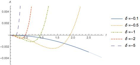
Figure 2: Effective anisotropy $A_{\delta}(t)$ as a function of $t$, for $S=10$ and different values of negative $\delta$, as indicated. The curve for $\delta=-0.1$ fades when the validity of the results is not fully under control (specifically for $t>S/4$).

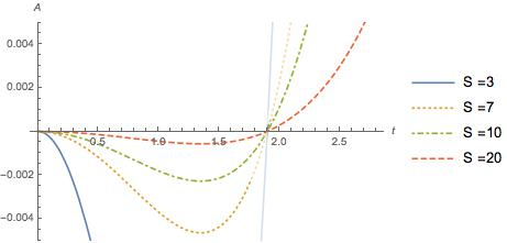
Figure 3: Effective anisotropy $A_{\delta}(t)$ as a funcion of $t$, for $\delta=-0.5$ and different values of $S$, as indicated. Lines as in Fig.2.

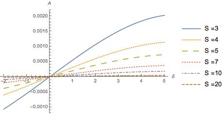
Figure 4: Effective anisotropy $A_{\delta}(t)$ as a function of $\delta$, for $t=0.1$ and different values of $S$, as indicated.

In the above comments, and figures 2-3, we have considered the case of negative detuning, $h<\omega$. The opposite case, $h>\omega$, trivially follows from $A_{\delta}(t)=-A_{-\delta}(t)$, as seen from the expression of $G_{\delta}(t)$ in the Appendix, as well as from Fig. 4, where we see that the effective anisotropy at a given time is an odd function of $\delta$, for all values of $S$.

V The evolved state

The factorized form of the propagator Eqs. (22-25) allows us to identify, amongst the overall effects of the interaction between $\Gamma$ and $\Xi$, those that do not generate entanglement between the twos. This is better seen and understood considering the evolved state for the entire system $\Psi=\Gamma\cup\Xi$, assuming its initial state $|{\Psi(0)}\rangle$ be separable, i.e. $|{\Psi(0)}\rangle=|{\Gamma}\rangle\otimes|{\Xi}\rangle$ (we will hereafter understand the symbol $\otimes$ whenever possible). From Eqs. (28-30) we get

$$|{\Psi(t)}\rangle = e^{-i\hat{H}t}|{\Gamma}\rangle|{\Xi}\rangle\sim$$ (32)

$$\sim e^{g(f_{\delta}(t)\hat{a}\hat{S}^{+}-f_{\delta}^{*}(t)\hat{a}^{\dagger}\hat{S}^{-})}e^{-i\omega\hat{a}^{\dagger}\hat{a}t}|{\Gamma}\rangle$$

$$\otimes\;e^{-i\int_{0}^{t}\hat{X}^{\rm eff}_{\Xi}(\tau)\,d\tau}|{\Xi}\rangle\sim$$

$$\sim e^{g(f_{\delta}(t)\hat{a}\hat{S}^{+}-f_{\delta}^{*}(t)\hat{a}^{\dagger}\hat{S}^{-})}|{\Gamma(t)}\rangle|{\tilde{\Xi}(t)}\rangle~{},$$

where $|{\Gamma(t)}\rangle=e^{-i\omega\hat{a}^{\dagger}\hat{a}t}|{\Gamma}\rangle$ and $|{\tilde{\Xi}(t)}\rangle=\exp[-i\int_{0}^{t}\hat{X}^{\rm eff}_{\Xi}(\tau)\,d\tau]|{\Xi}\rangle$ describe the free evolution of the bosonic system and the effective free evolution of the magnetic one, respectively. We have used the notation $|{\tilde{\Xi}(t)}\rangle$ to underline that while $|{\Gamma(t)}\rangle$ does not depend on the interaction between $\Gamma$ and $\Xi$, the evolution of $|{\tilde{\Xi}(t)}\rangle$ is induced not only by the free Hamiltonian $h\hat{S}_{z}$, but also by the back-action $g^{2}G_{\delta}(t)\hat{S}^{+}\hat{S}^{-}$ that follows from its coupling with $\Gamma$.

In the above expression (32) we can recognize a sort of interaction picture with two distinct rotating frames, one for the principal system and one for the environment, that do not move independently. In particular, it is the latter that changes its pace according to the continuous update of the non-commuting components of the environmental magnetic moment implied by an interaction of the TC form. It is worth noticing, to this respect, that the spin commutation relations, that in our case are the obstacle to the adoption of an exact interaction picture and the reason why an approximation scheme must be adopted, effectively manifest themselves in the non trivial time-dependence of the back-action, to represent their essential role in the quantum dynamics generated by the Hamiltonian (2).

Reminding that $G$ is pure imaginary, in Fig. 5 we plot $g^{2}|G_{\delta}(t)|$ as a function of time for $\delta=-0.5$ and $S=3,10$. Its behaviour qualitatively shows that the back-action has its maximum effect, at least as far as the time-interval where our approximation holds, for $t\simeq 1/|\delta|$ and vanishes for $t>\simeq 1/|\delta|$, no matter the value of the $S$.

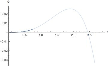
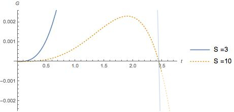
Figure 5: The back-action $g^{2}|G_{\delta}(t)|$ for $\delta=-0.5$ and different values of $S$; the inset shows the $S=3$ case in its proper plot-range. Lines as in Fig. 2.

Let us finally focus our attention upon the environmental reduced density matrix; writing the projector $\varrho(t)=|{\Psi(t)}\rangle\langle{\Psi(t)}|$ and tracing out the $\Gamma$-degrees of freedom, we get

$$\varrho_{\Xi}(t)\sim\sum_{\gamma}\hat{O}^{{\gamma,\Gamma}}_{{\Xi}}(t)|{\tilde{\Xi}(t)}\rangle\langle{\tilde{\Xi}(t)}|\hat{O}^{{\gamma,\Gamma}\;\dagger}_{{\Xi}}(t)\;,$$ (33)

where we have defined the operators

$$\hat{O}^{\gamma}_{\Xi}(t)\equiv\hat{O}^{\gamma}_{\Xi}(t;|{\Gamma(t)}\rangle)\equiv\langle{\gamma}|e^{g(f_{\delta}(t)\hat{a}\hat{S}^{+}-f_{\delta}^{*}(t)\hat{a}^{\dagger}\hat{S}^{-})}|{\Gamma(t)}\rangle\;$$ (34)

and $\{|{\gamma}\rangle\}$ is an orthonormal basis on $\mathcal{H}_{\Gamma}$. The set of operators $\{\hat{O}^{\gamma}_{\Xi}(t)\}$ acting on the Hilbert space of the environment can be interpreted as one set of Kraus operators (Nielsen and Chuang, 2004), since the completeness relation

$$\sum_{\gamma}\hat{O}^{\gamma\dagger}_{{\Xi}}(t)\hat{O}^{\gamma}_{{\Xi}}(t)=\hat{\mathbb{I}}_{\Xi}$$ (35)

holds for all $t$, as one can easily verify. The fact that the emerging Kraus operators do not depend on $G_{\delta}(t)$ is fully consistent with the fact that the back-action does not generate entanglement, as commented above, and rather dinamically renormalizes the environmental free Hamiltonian $\hat{H}^{\rm eff}_{\Xi}(t)$. We do also notice that, in order for the back-action to have a non trivial effect on the environment, the initial state $|{\Xi(0)}\rangle$ must be different from whatever eigenstate of $\hat{S}^{z}$, to avoid the anisotropy term in $\hat{X}^{\rm eff}_{\delta}(t)$ to affect $|{\tilde{\Xi}(t)}\rangle$ only by a phase factor.

VI Conclusions

In this concluding section we gather the information obtained so far in order to devise a strategy that make the dynamics of $\Xi$ the most sensitive possible to its interaction with $\Gamma$. In fact, as mentioned in the Introduction, if $\Xi$ is the measuring instrument used for getting information on, or exert our control upon, the quantum system $\Gamma$, one such strategy might reveal details, or allow a steering precision, otherwise inaccessible. To this respect, the lesson learnt in this work goes as follows.

1) Detuning: $\delta=h-\omega$ must be finite if one wants to observe footprints of $\Gamma$ into an effectively-free evolution of $\Xi$, i.e. without further interacting with $\Gamma$ itself. Off-resonance is a necessary condition for the back-action to switch on.

2) Timing: depending on the value of $\delta$ and $S$, there exist a finite time interval, that can be well within the range of validity of our results as shown in Figs. 2-5, where the back-action is larger, meaning that effects of $\Gamma$ on the dynamics of $\Xi$ could be more pronounced.

3) Magnetic properties: although our results are obtained in the large-$S$ approximation, it is important that $S$ stays finite, to avoid the disentangled dynamics of $\Xi$ to be just a silent Larmor precession. For the same reason, it is important that $\Xi$ be prepared in an initial state which is not an eigenstate of $\hat{S}^{z}$: significantly, in Ref. Foti (2015) we have seen that spin coherent states (Lieb, 1973; Gilmore, 1972) might be a particularly significant choice.

We conclude by mentioning that the method here used for implementing the large-$S$ approximation, i.e. making explicit the dependence of the spin-algebra on the quanticity parameter $1/S$ and then requiring the interaction Hamiltonian to stay finite as such parameter drops, is general and might turn useful in studying other quantum systems with several interacting components, amongst which a macroscopic one, furthermore preserving the geometry of the spin-sphere.

*

Appendix A

The results of points i)-ii) of Sec.III.2 are obtained by the repeated use of Eq. (18), realizing in Eq. (19) with

$$K_{1\delta}(\lambda) = \frac{1}{\delta^{2}}\sum_{m\geq 1}\frac{2m}{(2m+1)!}\lambda^{2m+1}\delta^{2m+1}$$ (36)

$$= \frac{1}{\delta^{2}}\left(-it\delta\cos t\delta+i\sin t\delta\right)~{},$$

and Eq. (III.2) with

$$K_{2\delta}(\lambda)=K_{1\delta}(\lambda)-\frac{1}{4\delta^{2}}\sum_{n\geq 1}(-1)^{n}\left[\frac{\lambda^{n}\delta^{n}}{n!}\right]^{2}\;.$$ (37)

As for the point iii), in order to group together all the terms proportional to $\hat{Y}^{+}$ ($\hat{Y}^{-}$), we perform the necessary $\hat{Y}^{+}\leftrightarrow\hat{Y}^{-}$ permutations in the infinite product of exponentials entering Eq. (III.2), and get

$$\exp\left[\lambda(\hat{Y}+\hat{X})\right]\sim$$ (38)

$$\sim \exp\left[\frac{1}{\delta}\sum_{n\geq 1}\frac{\lambda^{n}\delta^{n}}{n!}\hat{Y}^{+}\right]\exp\left[-\frac{1}{\delta}\;\sum_{n\geq 1}\frac{(-\lambda)^{n}\delta^{n}}{n!}\hat{Y}^{-}\right]$$

$$\times\exp\left[-2g^{2}K_{2\delta}(\lambda)\hat{S}^{+}\hat{S}^{-}\right]$$

$$\times\exp\left[\zeta_{\delta}(\lambda)g^{2}\hat{S}^{+}\hat{S}^{-}\right]\exp\left(\lambda\hat{X}\right)~{},$$

where $\zeta_{\delta}(\lambda)$ is the coefficient resulting from the commutators $[\hat{Y}^{+},\hat{Y}^{-}]$, introduced while moving all the $\hat{Y}^{-}$ to the right.

In order to determine $\zeta_{\delta}(\lambda)$, we consider

$$e^{\mu\hat{Y}^{-}}e^{\pi\hat{Y}^{+}}\sim e^{\mu\hat{Y}^{-}+\pi\hat{Y}^{+}+\frac{1}{2}\mu\pi[\hat{Y}^{-},\hat{Y}^{+}]}=$$

$$=e^{\pi\hat{Y}^{+}}e^{\mu\hat{Y}^{-}}e^{-\mu\pi[\hat{Y}^{+},\hat{Y}^{-}]}=e^{\pi\hat{Y}^{+}}e^{\mu\hat{Y}^{-}}e^{-\mu\pi g^{2}\hat{S}^{+}\hat{S}^{-}}\;$$ (39)

and define

$$\pi_{n}=\frac{\lambda^{n}\delta^{n}}{n!\delta}\;\;\;\mbox{and}\;\;\;\mu_{n}=-\;\frac{(-\lambda)^{n}\delta^{n}}{n!\delta}\;,$$ (40)

so that the expression from which we will get $\zeta_{\delta}(\lambda)$ (see Eq. (38)) reads

$$\cdots\;e^{\mu_{\ell+1}\hat{Y}^{-}}\;e^{\pi_{\ell}\hat{Y}^{+}}\;\cdots\;e^{\mu_{3}\hat{Y}^{-}}\;e^{\pi_{2}\hat{Y}^{+}}\;e^{\mu_{2}\hat{Y}^{-}}\;e^{\pi_{1}\hat{Y}^{+}}e^{\mu_{1}\hat{Y}^{-}}\;.$$ (41)

We then need to exchange every $\pi_{n}\hat{Y}^{+}$ with all the $\mu_{\ell}\hat{Y}^{-}$ of the following orders, i.e. such that $n>\ell$: after the first permutation we get

$$\cdots\;e^{\mu_{\ell+1}\hat{Y}^{-}}\;e^{\pi_{\ell}\hat{Y}^{+}}\;\cdots\;e^{\pi_{3}\hat{Y}^{+}}e^{\mu_{3}\hat{Y}^{-}}$$

$$\underbrace{e^{\pi_{2}\hat{Y}^{+}}e^{\pi_{1}\hat{Y}^{+}}}_{e^{(\pi_{1}+\pi_{2})\hat{Y}^{+}}}e^{\mu_{2}\hat{Y}^{-}}e^{-\mu_{2}\pi_{1}g^{2}\hat{S}^{+}\hat{S}^{-}}e^{\mu_{1}\hat{Y}^{-}}\;,$$ (42)

and one can easily check that successive permutations give the terms

$$e^{-\mu_{2}\pi_{1}g^{2}\hat{S}^{+}\hat{S}^{-}}$$

$$e^{-\mu_{3}(\pi_{1}+\pi_{2})g^{2}\hat{S}^{+}\hat{S}^{-}}$$

$$\vdots$$

$$e^{-\mu_{\ell+1}(\pi_{1}+\pi_{2}+\pi_{3}+...+\pi_{\ell})g^{2}\hat{S}^{+}\hat{S}^{-}}\;,$$

so that

$$\exp\left[\zeta_{\delta}(\lambda)g^{2}\hat{S}^{+}\hat{S}^{-}\right]\sim$$

$$\sim\exp\left[-\left(\sum_{\ell\geq 2}\mu_{\ell}\sum_{1\leq j<\ell}\pi_{j}\right)g^{2}\hat{S}^{+}\hat{S}^{-})\right]=$$

$$=\exp\left[\frac{1}{\delta^{2}}\left(\sum_{\ell\geq 2}\frac{(-\lambda)^{\ell}\delta^{\ell}}{\ell!}\sum_{1\leq j<\ell}\frac{\lambda^{j}\delta^{j}}{j!}\right)g^{2}\hat{S}^{+}\hat{S}^{-}\right]\;.$$

Therefore, from Eq. (21), it is

$$K_{3\delta}(\lambda)=-2K_{2\delta}(\lambda)+\zeta_{\delta}(\lambda)=$$ (44)

$$= -2K_{2\delta}(\lambda)+\frac{1}{\delta^{2}}\sum_{\ell\geq 2}\frac{(-\lambda)^{\ell}\delta^{\ell}}{\ell!}\sum_{1\leq j<\ell}\frac{\lambda^{j}\delta^{j}}{j!}=$$

$$= -2K_{1\delta}(\lambda)+\frac{1}{2\delta^{2}}\sum_{n\geq 1}\frac{(-\lambda\delta)^{n}}{n!}\frac{(\lambda\delta)^{n}}{n!}+$$

$$+\frac{1}{\delta^{2}}\sum_{\ell\geq 2}\frac{(-\lambda\delta)^{\ell}}{\ell!}\sum_{1\leq j<\ell}\frac{(\lambda\delta)^{j}}{j!}~{}.$$

Being $\lambda=-it$, we notice that $-\lambda=\lambda^{*}$ and set $x=\lambda\delta$, $x^{*}=\lambda^{*}\delta$; the last two terms can be written as

$$\frac{1}{\delta^{2}}\left(\frac{1}{2}\sum_{n\geq 1}\frac{x^{*n}}{n!}\frac{x^{n}}{n!}+\sum_{\ell\geq 2}\frac{x^{*\ell}}{\ell!}\sum_{1\leq j<\ell}\frac{x^{j}}{j!}\right)=$$ (45)

$$= \frac{1}{2\delta^{2}}\sum_{n\geq 1}\frac{x^{n}}{n!}\sum_{\ell\geq 1}\frac{x^{*\ell}}{\ell!}-\frac{1}{2\delta^{2}}\sum_{n\geq 1}\frac{x^{n}}{n!}\sum_{\ell\neq n}\frac{x^{*\ell}}{\ell!}+$$

$$+\frac{1}{\delta^{2}}\sum_{\ell\geq 2}\frac{x^{*\ell}}{\ell!}\sum_{1\leq j<\ell}\frac{x^{j}}{j!}$$

$$= \frac{1}{2}|f_{\delta}(\lambda)|^{2}+M_{\delta}(\lambda)~{},$$

where, going back to $\lambda$ and $\delta$, the first serie can be written in terms of $f_{\delta}(\lambda)\equiv(e^{\lambda\delta}-1)/\delta$, i.e. the function defined in Eq. (23), and

$$M_{\delta}(\lambda) = -\frac{1}{2\delta^{2}}\sum_{n\geq 1}\frac{(\lambda\delta)^{n}}{n!}\sum_{\ell\neq n}\frac{(\lambda^{*}\delta)^{\ell}}{\ell!}+$$ (46)

$$+\frac{1}{\delta^{2}}\sum_{\ell\geq 2}\frac{(\lambda^{*}\delta)^{\ell}}{\ell!}\sum_{1\leq j<\ell}\frac{(\lambda\delta)^{j}}{j!}~{}.$$

The propagator (38) is then

$$\exp\left[\lambda(\hat{Y}+\hat{X})\right]\sim$$ (47)

$$\sim \exp\left[f_{\delta}(\lambda)\hat{Y}^{+}\right]\exp\left[-f^{*}_{\delta}(\lambda)\hat{Y}^{-}\right]$$

$$\times\exp\left(K_{3\delta}(\lambda)g^{2}\hat{S}^{+}\hat{S}^{-}\right)\exp\left(\lambda\hat{X}\right)$$

$$\sim \exp\left[f_{\delta}(\lambda)\hat{Y}^{+}-f^{*}_{\delta}(\lambda)\hat{Y}^{-}\right]\exp\left(-\frac{1}{2}|f_{\delta}(\lambda)|^{2}g^{2}\hat{S}^{+}\hat{S}^{-}\right)$$

$$\times\exp\left(K_{3\delta}(\lambda)g^{2}\hat{S}^{+}\hat{S}^{-}\right)\exp\left(\lambda\hat{X}\right)~{},$$

where in the last step we have used $e^{f_{\delta}(\lambda)\hat{Y}^{+}}e^{-f^{*}_{\delta}(\lambda)\hat{Y}^{-}}\sim e^{f_{\delta}(\lambda)\hat{Y}^{+}-f^{*}_{\delta}(\lambda)\hat{Y}^{-}-\frac{1}{2}\left|f_{\delta}(\lambda)\right|^{2}[\hat{Y}^{+},\hat{Y}^{-}]}$ and Eq. (15). Looking at Eq. (24), we therefore have

$$G_{\delta}(\lambda)=K_{3\delta}(\lambda)-\frac{1}{2}|f_{\delta}(\lambda)|^{2}=-2K_{1\delta}(\lambda)+M_{\delta}(\lambda)~{}.$$ (48)

We now want to show that the above expression is a pure imaginary one; since $K_{1\delta}(\lambda)\in\Im$, this means actually to show that $M_{\delta}(\lambda)\in\Im$. Restoring $x=\lambda\delta$ and $x^{*}=\lambda^{*}\delta$ to have a simpler notation, we have

$$M(x) = -\frac{1}{2\delta^{2}}\sum_{n\geq 1}\frac{x^{n}}{n!}\sum_{\ell\neq n}\frac{x^{*\ell}}{\ell!}+\frac{1}{\delta^{2}}\sum_{\ell\geq 2}\frac{x^{*\ell}}{\ell!}\sum_{1\leq j<\ell}\frac{x^{j}}{j!}=$$

$$= -\frac{1}{2\delta^{2}}\sum_{n\geq 1}\frac{x^{n}}{n!}\sum_{\ell>n}\frac{x^{*\ell}}{\ell!}-\frac{1}{2\delta^{2}}\sum_{n\geq 2}\frac{x^{n}}{n!}\sum_{1\leq\ell<n}\frac{x^{*\ell}}{\ell!}$$

$$+\frac{1}{2\delta^{2}}\sum_{\ell\geq 2}\frac{x^{*\ell}}{\ell!}\sum_{1\leq j<\ell}\frac{x^{j}}{j!}+\frac{1}{2\delta^{2}}\sum_{\ell\geq 2}\frac{x^{*\ell}}{\ell!}\sum_{1\leq j<\ell}\frac{x^{j}}{j!}~{}.$$

One can easily verify that the first and the third term sum up to zero, therefore it is

$$M(x)=-\frac{1}{2\delta^{2}}\sum_{n\geq 2}\frac{x^{n}}{n!}\sum_{1\leq\ell<n}\frac{x^{*\ell}}{\ell!}+\frac{1}{2\delta^{2}}\sum_{\ell\geq 2}\frac{x^{*\ell}}{\ell!}\sum_{1\leq j<\ell}\frac{x^{j}}{j!}~{},$$ (50)

and, noticing that the expression above is nothing but the sum of the quantity $-\frac{1}{2\delta^{2}}\sum_{n\geq 2}\frac{x^{n}}{n!}\sum_{1\leq\ell<n}\frac{x^{*\ell}}{\ell!}$ with its complex conjugate, we have $M(x)\in\Im$: this implies that only the odd terms (looking at the exponents $n+\ell$ as powers of $t\delta$) survive in the sum of the two series above. Finally, going back at Eq. (48), we get the pure imaginary quantity

$$G_{\delta}(t) = i{\Big{\{}}-\frac{1}{\delta^{2}}{\Big{[}}-2t\delta\cos t\delta+2\sin t\delta+$$

$$+\Im{\rm m}{\Big{(}}\sum_{n\geq 2}\frac{(-it\delta)^{n}}{n!}\sum_{1\leq\ell<n}\frac{(it\delta)^{\ell}}{\ell!}{\Big{)}}{\Big{]}}{\Big{\}}}\;,$$

where the real time $t$ is back. This is the back-action term Eq. (24) defined and analyzed in Sec. III.1.

References

• Schlosshauer (2007) M. Schlosshauer, Decoherence and the Quantum-To-Classical Transition, The Frontiers Collection (Springer, 2007).
• Rivas and Huelga (2012) A. Rivas and S. F. Huelga, Open Quantum Systems: An Introduction (Springer Berlin Heidelberg, 2012).
• Breuer and Petruccione (2002) H. P. Breuer and F. Petruccione, The theory of open quantum systems (Oxford University Press, Great Clarendon Street, 2002).
• Paladino et al. (2002) E. Paladino, L. Faoro, G. Falci, and R. Fazio, Phys. Rev. Lett. 88, 228304 (2002), URL http://link.aps.org/doi/10.1103/PhysRevLett.88.228304.
• Lo Franco et al. (2013) R. Lo Franco, B. Bellomo, S. Maniscalco, and G. Compagno, Int. J. Mod. Phys. B 27, 1345053 (2013).
• Xu et al. (2013) J.-S. Xu, K. Sun, C.-F. Li, X.-Y. Xu, G.-C. Guo, E. Andersson, R. Lo Franco, and G. Compagno, Nat Commun 4, (2013), URL http://dx.doi.org/10.1038/ncomms3851.
• Matsumoto (2015) N. Matsumoto, Classical Pendulum Feels Quantum Back-Action, Springer Theses (Springer, 2015), ISBN 4431558802,9784431558804.
• Kippenberg and Vahala (2008) T. J. Kippenberg and K. J. Vahala, Science 321, 1172 (2008), ISSN 0036-8075, URL http://science.sciencemag.org/content/321/5893/1172.
• Verhagen et al. (2012) E. Verhagen, S. Deleglise, S. Weis, A. Schliesser, and T. J. Kippenberg, Nature 482, 63 (2012), ISSN 0028-0836, URL http://dx.doi.org/10.1038/nature10787.
• Lieb (1973) E. H. Lieb, Communications in Mathematical Physics 31, 327 (1973), URL http://projecteuclid.org/euclid.cmp/1103859040.
• Palma et al. (1996) G. M. Palma, K.-A. Suominen, and A. K. Ekert, Proceedings of the Royal Society of London. Series A: Mathematical, Physical and Engineering Sciences 452, 567 (1996), URL http://rspa.royalsocietypublishing.org/content/452/1946/567.abstract.
• Cucchietti et al. (2010) F. M. Cucchietti, J.-F. Zhang, F. C. Lombardo, P. I. Villar, and R. Laflamme, Phys. Rev. Lett. 105, 240406 (2010), URL http://link.aps.org/doi/10.1103/PhysRevLett.105.240406.
• Fernando Casas (2012) M. N. Fernando Casas, Ander Murua, Computer Physics Communications 20 (2012).
• Zassenhaus (1939) H. Zassenhaus, in Abhandlungen aus dem Mathematischen Seminar der Universität Hamburg (1939), vol. 13, pp. 1–100.
• Tavis and Cummings (1968) M. Tavis and F. W. Cummings, Phys. Rev. 170, 379 (1968), URL http://link.aps.org/doi/10.1103/PhysRev.170.379.
• Yaffe (1982) L. G. Yaffe, Rev. Mod. Phys. 54, 407 (1982), URL http://link.aps.org/doi/10.1103/RevModPhys.54.407.
• Garraway (2011) B. M. Garraway, Phil. Trans. R. Soc. A 20 (2011).
• Bennett et al. (2013) S. D. Bennett, N. Y. Yao, J. Otterbach, P. Zoller, P. Rabl, and M. D. Lukin, Phys. Rev. Lett. 110, 156402 (2013), URL http://link.aps.org/doi/10.1103/PhysRevLett.110.156402.
• Härkönen et al. (2009) K. Härkönen, F. Plastina, and S. Maniscalco, Phys. Rev. A 80, 033841 (2009), URL http://link.aps.org/doi/10.1103/PhysRevA.80.033841.
• Feng et al. (2015) M. Feng, Y. Zhong, T. Liu, L. Yan, W. Yang, J. Twamley, and H. Wang, Nat Commun 6, (2015), URL http://dx.doi.org/10.1038/ncomms8111.
• Paladino et al. (2014) E. Paladino, Y. M. Galperin, G. Falci, and B. L. Altshuler, Rev. Mod. Phys. 86, 361 (2014), URL http://link.aps.org/doi/10.1103/RevModPhys.86.361.
• Benedetti et al. (2013) C. Benedetti, F. Buscemi, P. Bordone, and M. G. A. Paris, Phys. Rev. A 87, 052328 (2013), URL http://link.aps.org/doi/10.1103/PhysRevA.87.052328.
• Wold et al. (2012) H. J. Wold, H. Brox, Y. M. Galperin, and J. Bergli, Phys. Rev. B 86, 205404 (2012), URL http://link.aps.org/doi/10.1103/PhysRevB.86.205404.
• (24) It might seem that the same reasoning should also hold for the external field $h$, but that is actually a different issue: the role of $h$ is that of defining an energy scale for the magnetic system, and the free Hamiltonian stays physical in the $S\rightarrow\infty$ limit.
• Mattis (1981-) D. C. Mattis, The theory of magnetism - Vol I (Springer-Verlag, Berlin ; New York, 1981-).
• Nielsen and Chuang (2004) M. A. Nielsen and I. L. Chuang, Quantum Computation and Quantum Information (Cambridge Series on Information and the Natural Sciences) (Cambridge University Press, 2004), 1st ed., ISBN 0521635039.
• Foti (2015) C. Foti, Ph.D. thesis, University of Florence (2015).
• Gilmore (1972) R. Gilmore, Annals of Physics 74, 391 (1972), ISSN 0003-4916, URL http://www.sciencedirect.com/science/article/pii/0003491672901479.