Reachability for dynamic parametric processes

Abstract

In a dynamic parametric process every subprocess may spawn arbitrarily many, identical child processes, that may communicate either over global variables, or over local variables that are shared with their parent. We show that reachability for dynamic parametric processes is decidable under mild assumptions. These assumptions are e.g. met if individual processes are realized by pushdown systems, or even higher-order pushdown systems. We also provide algorithms for subclasses of pushdown dynamic parametric processes, with complexity ranging between NP and DEXPTIME.

1 Introduction

Programming languages such as Java, Erlang, Scala offer the possibility to generate recursively new threads (or processes, actors,…). Threads may exchange data through globally accessible data structures, e.g. via static attributes of classes like in Java, Scala. In addition, newly created threads may locally communicate with their parent threads, in Java, e.g., via the corresponding thread objects, or via messages like in Erlang.

Various attempts have been made to analyze systems with recursion and dynamic creation of threads that may or may not exchange data. A single thread executing a possibly recursive program operating on finitely many local data, can conveniently be modeled by a pushdown system. Intuitively, the pushdown formalizes the call stack of the program while the finite set of states allows to formalize the current program state together with the current values of the local variables. For such systems reachability of a bad state or a regular set of bad configurations is decidable [17, 1]. The situation becomes more intricate if multiple threads are allowed. Already for two pushdown threads reachability is undecidable if communication via a 2-bit global is allowed. In absence of global variables, reachability becomes undecidable already for two pushdown threads if a rendez-vous primitive is available [16]. A similar result holds if finitely many locks are allowed [10]. Interestingly, decidability is retained if locking is performed in a disciplined way. This is, e.g., the case for nested [10] and contextual locking [3]. These decidability results have been extended to dynamic pushdown networks as introduced by Bouajjani et al. [2]. This model combines pushdown threads with dynamic thread creation by means of a spawn operation, while it ignores any exchange of data between threads. Indeed, reachability of dedicated states or even regular sets of configurations stays decidable in this model, if finitely many global locks together with nested locking [12, 14] or contextual locking [13] are allowed. Such regular sets allow, e.g., to describe undesirable situations such as concurrent execution of conflicting operations.

Here, we follow another line of research where models of multi-threading are sought which allow exchange of data via shared variables while still being decidable. The general idea goes back to Kahlon, who observed that various verification problems become decidable for multi-pushdown systems that are parametric [9], i.e., systems consisting of an arbitrary number of indistinguishable pushdown threads. Later, Hague extended this result by showing that an extra designated leader thread can be added without sacrificing decidability [7]. All threads communicate here over a shared, bounded register without locking. It is crucial for decidability that only one thread has an identity, and that the operations on the shared variable do not allow to elect a second leader. Later, Esparza et al. clarified the complexity of deciding reachability in that model [5]. La Torre et al. generalized these results to hierarchically nested models [11]. Still, the question whether reachability is decidable for dynamically evolving parametric pushdown processes, remained open.

We show that reachability is decidable for a very general class of dynamic processes with parametric spawn. We require some very basic properties from the class of transitions systems that underlies the model, like e.g. effective non-emptiness check. In our model every sub-process can maintain e.g. a pushdown store, or even a higher-order pushdown store, and can communicate over global variables, as well as via local variables with its sub-processes and with its parent. As in [7, 5, 11], all variables have bounded domains and no locks are allowed.

Since the algorithm is rather expensive, we also present meaningful instances where reachability can be decided by simpler means. As one such instance we consider the situation where communication between sub-processes is through global variables only. We show that reachability for this model with pushdowns can effectively be reduced to reachability in the parametric model of Hague [7, 5], called $(C,D)$-systems — giving us a precise characterization of the complexity as Pspace. As another instance, we consider a parametric variant of generalized futures where spawned sub-processes may not only return a single result but create a stream of answers. For that model, we obtain complexities between NP and DExptime. This opens the venue to apply e.g. SAT-solving to check safety properties of such programs.

Overview. Section 2 provides basic definitions, and the semantics of our model. In Section 3 we show a simpler semantics, that is equivalent w.r.t. reachability. Section 4 introduces some prerequisites for Section 5, which is the core of the proof of our main result. Section 6 considers the complexity for some special instances of dynamic parametric pushdown processes.

2 Basic definitions

In this section we introduce our model of dynamic parametric processes. We refrain from using some particular program syntax; instead we use potentially infinite state transition systems with actions on transitions. Actions may manipulate local or global variables, or spawn parametrically some sub-processes: this means that an unspecified number of sub-processes is created — all with the same designated initial state. Making the spawn operation parametric is the main abstraction step that allows us to obtain decidability results.

Before giving formal definitions we present two examples in order to give an intuitive understanding of the kind of processes we are interested in.

Example 1

A parametric system could, e.g., be defined by an explicitly given finite transition system:

In this example, the root starts in state $q$ by spawning a number of sub-processes, each starting in state $p$. Then the root writes the value 1 into the local variable $x$, and waits for some child to change the value of $x$ first to $2$, and subsequently to $3$. Only then, the root will write value $\#$ into the global variable $g_{0}$. Every child on the other hand, when starting execution at state $p$, waits for value $1$ in the variable $x$ of the parent and then chooses either to write $2$ or $3$ into $x$, then returns to the initial state. The read/write operations of the children are denoted as input/output operations $\mathit{i}(x,v),\mathit{o}(x,v)$, because they act on the parent’s local. Note that at least two children are required to write $\#$.

More interesting examples require more program states. Here, it is convenient to adopt a programming-like notation as in the next example.

Example 2

⬇

1root() {

spawn(p);

switch (x) {

4 case 2: write(#);

}

}

7

p() {

switch (parent.x) {

10 case 0 : spawn(p);

if (*) parent.x = 1

else switch (x) {

13 case 1 : parent.x = 1; break;

case 2 : break;

}; break;

16 case 1 : spawn(p);

if (*) parent.x = 0

else switch (x) {

19 case 1: parent.x = 2; break;

case 2: parent.x = 2; break;

};

22 }

}

Figure 1: A program defining a dynamic parametric process.

Consider the program from Figure 1. The states of the system correspond to the lines in the listing, and $\textsf{if}(*)$ denotes non-deterministic choice. There is a single global variable which is written to by the call write(#), and a single local variable $x$ per sub-process, with initial value 0. The corresponding local of the parent is accessed via the keyword parent.

The question is whether the root can eventually write #? This would be the case if the value of the root’s local variable becomes 2. This in turn may occur once the variable x of some descendant is set to 1. In order to achieve this, cooperation of several sub-processes is needed. Here is one possible execution.

1. The root spawns two sub-processes in state $p$, say $T_{1}$ and $T_{2}$.

2. $T_{1}$ changes the value of the local variable of the root to 1 (line 11).

3. $T_{2}$ then can take the case 1 branch and first spawn $T_{3}$.

4. $T_{3}$ takes the case 0 branch, spawns a new process and changes the value of parent.x to 1.

5. As the variable parent.x of $T_{3}$ is the local variable of $T_{2}$, the latter can now take the second branch of the nondeterministic choice and change parent.x to 2 (line 19) — which is the local variable of the root.

∎

In the following sections we present a formal definition of our parametric model, state the reachability problem, and the main results. This is done in three steps. In the first subsection, we introduce the syntax that will be given in a form of a transition system, as the one from the first example. Next, we give the formal operational semantics that captures the behavior described in the above examples. Finally, we formulate general requirements on a class of systems and state the result saying that for every class satisfying these requirements, the reachability problem for the associated dynamic parametric processes is decidable.

2.1 Transition systems

A dynamic parametric process $\mathcal{S}$ is a transition system over a dedicated set of action names. One can think of it as a control flow graph of a program. In this transition system the action names are uninterpreted. In Section 2.2 we will define their semantics. Such a transition system can be obtained by symbolically executing a program, say, expanding while loops and procedure calls. Another possibility is that the control flow of a program is given by a pushdown automaton; in this case the transition system will have configurations of the pushdown automaton as states.

The transition system is specified by a tuple $\mathcal{S}=\langle Q,G,X,V,\Delta,q_{\mathsf{init}},v_{\mathsf{init}}\rangle$ consisting of:

• a (possibly infinite) set $Q$ of states,

• finite sets $G$ and $X$ of global and local variables, respectively, and a finite set $V$ of values for variables; these are used to define the set of labels,

• an initial state $q_{\mathsf{init}}\in Q$, and an initial value $v_{\mathsf{init}}\in V$ for variables,

• a set of rules $\Delta$ of the form $q\stackrel{{\scriptstyle a}}{{\longrightarrow}}q^{\prime}$, where the label $a$ is one of the following:

  • $\tau$, that will be later interpreted as a silent action,

  • $\mathit{r}(x,v)$, $\mathit{w}(x,v)$, will be interpreted as a read or a write of value $v\in V$ from or to a local or global variable $x\in X\cup G$ of the process,

  • $\mathit{i}(x,v)$, $\mathit{o}(x,v)$, will be interpreted as a read or a write of value $v\in V$ to or from a local variable $x\in X$ of the parent process,

  • ${\sf spawn}(q)$, will be interpreted as a spawn of an arbitrary number (possibly zero) of new sub-processes, all starting in state $q\in Q$. We assume that the number of different ${\sf spawn}(q)$ operations appearing in $\Delta$ is finite.

Observe that the above definition ensures that the set of labels of transitions is finite.

We are particularly interested in classes of systems when $Q$ is not finite. This is the case when, for example, individual sub-processes execute recursive procedures. For that purpose, the transition system $\mathcal{S}$ may be chosen as a configuration graph of a pushdown system. In this case the set $Q$ of states is $Q_{l}\cdot\Gamma^{*}$ where $Q_{l}$ is a finite set of control states, and $\Gamma$ is a finite set of pushdown symbols. The (infinite) transition relation $\Delta$ between states is specified by a finite set of rewriting rules of the form $qv\stackrel{{\scriptstyle a}}{{\longrightarrow}}q^{\prime}w$ for suitable $q,q^{\prime}\in Q_{l},v\in\Gamma^{*},w\in\Gamma^{*}$.

Instead of plain recursive programs, we could also allow higher-order recursive procedures, realized by higher-order pushdown systems or even collapsible pushdown systems as considered, e.g., in [15, 8]. Here, procedures may take other procedures as arguments.

2.2 Multiset semantics

A dynamic parametric process is a transition system with labels of a special form. As we have seen from the examples, such a transition system can be provided either directly, or as the configuration graph of a machine, or as the flow-graph of a program with procedure calls. In this subsection we provide the operational semantics of programs given by such transition systems, where we interpret the operations on variables as expected, and the spawns as creation of sub-processes. The latter operation will not create one sub-process, but rather an arbitrary number of sub-processes. There will be also a set of global variables to which every sub-process has access by means of reads and writes.

As a dynamic parametric process executes, sub-processes may change the values of local and global variables and spawn new children. The global state of the entire process can be thus represented as a tree of sub-processes with the initial process at the root. Nodes at depth 1 are the sub-processes spawned by the root; these children can also spawn sub-processes that become nodes at depth $2$, etc, see e.g., Figure 3(a). Every sub-process has a set of local variables, that can be read and written by itself, as well as by its children.

A global state of a dynamic parametric process $\mathcal{S}$ has the form of a multiset configuration tree, or m-tree for short. An m-tree is defined recursively by

$$\begin{array}[]{lll}t&{::=}&(q,\lambda,M)\end{array}$$

where $q\in Q$ is a sub-process state, $\lambda:X\to V$ is a valuation of (local) variables, and $M$ is a finite multiset of m-trees. We consider only m-trees of finite depth. Another way to say this is to define m-trees of depth at most $k$, for every $k\in\mathbb{N}$

$$\text{{M-trees}}_{0} = Q\times(X\to V)\times[]$$

$$\text{{M-trees}}_{k} = Q\times(X\to V)\times\mathcal{M}(\text{{M-trees}}_{k-1})\qquad\mbox{for $k>0$}$$

where for any $U$, $\mathcal{M}(U)$ is the set of all finite multisubsets of $U$. Then the set of all m-trees is given by $\bigcup_{k\in\mathbb{N}}\text{{M-trees}}_{k}$.

We use standard notation for multisets. A multiset $M$ over a universe $U$ is a mapping $M:U\to{\mathbb{N}}_{0}$. It is finite if $\sum_{t\in U}M(t)<\infty$. A finite multiset $M$ may also be represented by $M=[n_{1}\cdot t_{1},\ldots,n_{k}\cdot t_{k}]$ if $M(t_{i})=n_{i}$ for $i=1,\ldots,k$ and $M(t)=0$ otherwise. In particular, the empty multiset is denoted by $[]$. For convenience we may omit multiplicities $n_{i}=1$. We say that $t\in M$ whenever $M(t)\geq 1$, and $M\subseteq M^{\prime}$ whenever $M(t)\leq M^{\prime}(t)$ for all $t\in M^{\prime}$. Finally, $M+M^{\prime}$ is the mapping with $(M+M^{\prime})(t)=M(t)+M^{\prime}(t)$ for all $t\in U$. For convenience, we also allow the short-cut $[n_{1}\cdot t_{1},\ldots,n_{k}\cdot t_{k}]$ for $[n_{1}\cdot t_{1}]+\ldots+[n_{k}\cdot t_{k}]$, i.e., we allow also multiple occurrences of the same tree in the list. Thus, e.g., $[3\cdot t_{1},5\cdot t_{2},1\cdot t_{1}]=[4\cdot t_{1},5\cdot t_{2}]$.

The semantics of a dynamic parametric process $\mathcal{S}$ is a transition system denoted ${[\![\mathcal{S}]\!]}$. The states of ${[\![S]\!]}$ are m-trees, and the set of possible edge labels is:

$$\Sigma = \{\tau\}\cup\{{\sf spawn}\}\times Q\,\cup$$

$$\{\mathit{i}(x,v),\mathit{o}(x,v),\mathit{r}(y,v),\mathit{w}(y,v),\overline{\mathit{r}}(y,v),\overline{\mathit{w}}(y,v):$$

$$\qquad x\in X,\,y\in X\cup G,v\in V\}\,.$$

Notice that we have two new kinds of labels $\overline{\mathit{r}}(y,v)$ and $\overline{\mathit{w}}(y,v)$. These represent the actions of child sub-processes on global variables $y\in G$, or on the local variables $x\in X$ shared with the parent.

Throughout the paper we will use the notation

$$\Sigma_{\mathit{ext}}=\{\mathit{i}(x,v),\mathit{o}(x,v),\mathit{r}(g,v),\mathit{w}(g,v):x\in X,g\in G,v\in V\}$$

for the set of so-called external actions. They are called external because they concern either the global variables, or the local variables of the parent of the sub-process. Words in $\Sigma_{\mathit{ext}}^{*}$ will describe the external behaviors of a sub-process, i.e., the interactions with the external world.

The initial state is given by $t_{\mathsf{init}}=(q_{\mathsf{init}},\lambda_{\mathsf{init}},[])$, where $\lambda_{\mathsf{init}}$ maps all locals to the initial value $v_{\mathsf{init}}$. A transition between two states of ${[\![\mathcal{S}]\!]}$ (m-trees) $t_{1}\stackrel{{\scriptstyle a}}{{\Longrightarrow}}_{\mathcal{S}}t_{2}$ is defined by induction on the depth of m-trees. We will omit the subscript $\mathcal{S}$ for better readability. The definition is given in Figure 2.

External transitions:

$$\begin{array}[]{lllll}(q_{1},\lambda,M)&\stackrel{{\scriptstyle a}}{{\Longrightarrow}}&(q_{2},\lambda,M)&\text{ if $q_{1}\stackrel{{\scriptstyle a}}{{\longrightarrow}}q_{2}$}&\text{for $a\in\Sigma_{\mathit{ext}}$}\\ (q,\lambda,M_{1})&\stackrel{{\scriptstyle\overline{\mathit{r}}(g,v)}}{{\Longrightarrow}}&(q,\lambda,M_{2})&\text{ if }M_{1}\stackrel{{\scriptstyle\mathit{r}(g,v)}}{{\Longrightarrow}}M_{2}&\text{for $g\in G$}\\ (q,\lambda,M_{1})&\stackrel{{\scriptstyle\overline{\mathit{w}}(g,v)}}{{\Longrightarrow}}&(q,\lambda,M_{2})&\text{ if }M_{1}\stackrel{{\scriptstyle\mathit{w}(g,v)}}{{\Longrightarrow}}M_{2}&\text{for $g\in G$}\\ \end{array}$$

Internal transitions:

$$\begin{array}[]{llll}(q_{1},\lambda,M)&\stackrel{{\scriptstyle\tau}}{{\Longrightarrow}}&(q_{2},\lambda,M)&\text{if $q_{1}\stackrel{{\scriptstyle\tau}}{{\longrightarrow}}q_{2}$}\\ (q_{1},\lambda,M_{1})&\stackrel{{\scriptstyle{\sf spawn}(p)}}{{\Longrightarrow}}&(q_{2},\lambda,M_{2})&\text{if $q_{1}\stackrel{{\scriptstyle{\sf spawn}(p)}}{{\longrightarrow}}q_{2}$ and $M_{2}=M_{1}+[n\cdot(p,\lambda_{\mathsf{init}},[])]$}\;\text{for some}\;m\geq 0\\ (q_{1},\lambda,M)&\stackrel{{\scriptstyle\mathit{w}(x,v)}}{{\Longrightarrow}}&(q_{2},\lambda^{\prime},M)&\text{if $q_{1}\stackrel{{\scriptstyle\mathit{w}(x,v)}}{{\longrightarrow}}q_{2}$ and $\lambda^{\prime}=\lambda[v/x]$}\\ (q_{1},\lambda,M)&\stackrel{{\scriptstyle\mathit{r}(x,v)}}{{\Longrightarrow}}&(q_{2},\lambda,M)&\text{if $q_{1}\stackrel{{\scriptstyle\mathit{r}(x,v)}}{{\longrightarrow}}q_{2}$ and $v=\lambda(x)$}\\ (q,\lambda,M_{1})&\stackrel{{\scriptstyle\overline{\mathit{r}}(x,v)}}{{\Longrightarrow}}&(q,\lambda,M_{2})&\text{if $M_{1}\stackrel{{\scriptstyle\mathit{i}(x,v)}}{{\Longrightarrow}}M_{2}$ and $v=\lambda(x)$}\\ (q,\lambda,M_{1})&\stackrel{{\scriptstyle\overline{\mathit{w}}(x,v)}}{{\Longrightarrow}}&(q,\lambda^{\prime},M_{2})&\text{if $M_{1}\stackrel{{\scriptstyle\mathit{o}(x,v)}}{{\Longrightarrow}}M_{2}$ and $\lambda^{\prime}=\lambda[v/x]$}\\ \end{array}$$

Here, we say that

$$\begin{array}[]{lll}M_{1}&\stackrel{{\scriptstyle a}}{{\Longrightarrow}}&M_{2}\quad\text{for }a\in\Sigma_{\mathit{ext}}\end{array}$$

if there is a multi-subset $M_{1}=M^{\prime}+[n_{1}\cdot t_{1},\ldots,n_{r}\cdot t_{r}]$ (where the $t_{i}$ need not necessarily be distinct) and executions $t_{i}\stackrel{{\scriptstyle\alpha_{i}a}}{{\Longrightarrow}}t^{\prime}_{i}$ for $i=1,\ldots,r$ for sequences $\alpha_{i}\in(\Sigma\setminus\Sigma_{\mathit{ext}})^{*}$ and $M_{2}=M^{\prime}+[n_{1}\cdot t^{\prime}_{1},\ldots,n_{r}\cdot t^{\prime}_{r}]$.

Figure 2: Multiset semantics of dynamic parametric processes.

External transitions (cf. Figure 2) describe operations on external variables, be they global or local. If the actions come from child sub-processes then for technical convenience we add a bar to them. Thanks to adding a bar, a label determines the rule that has been used for the transition (This is important in Prop. 2). The values of global variables are not part of the program state. Accordingly, these operations therefore can be considered as unconstrained input/output actions.

Internal transitions may silently change the current state, spawn new sub-processes or update or read the topmost local variables of the process. The expression $\lambda[v/x]$ denotes the function $\lambda^{\prime}:X\to V$ defined by $\lambda^{\prime}(x^{\prime})=\lambda(x^{\prime})$ for $x^{\prime}\neq x$ and $\lambda^{\prime}(x)=v$. In the case of spawn, the initial state of the new sub-processes is given by the argument, while the fresh local variables are initialized with the default value. In the last two cases (cf. Figure 2) the external actions $\mathit{i}(x,v),\mathit{o}(x,v)$ of the child sub-processes get relabeled as the corresponding internal actions $\overline{\mathit{r}}(x,v),\overline{\mathit{w}}(x,v)$ on the local variables of the parent.

We write $t_{1}\stackrel{{\scriptstyle\alpha}}{{\Longrightarrow}}t_{2}$ for a sequence of transitions complying with the sequence $\alpha$ of action labels. We have chosen the option to allow several child sub-processes to move in one step. While this makes the definition slightly more complicated, it simplifies some arguments later. Observe that the semantics makes the actions (labels) at the top level explicit, while the actions of child sub-processes are explicit only if they refer to globals or affect the local variables of the parent.

2.3 Problem statement and main result

In this section we define the reachability problem and state our main theorem: it says that the reachability problem is decidable for dynamic parametric processes built upon an admissible class of systems. The notion of admissible class will be introduced later in this section. Before we do so, we introduce a consistency requirement for runs of parametric processes. In our semantics we have chosen not to constrain the operations on global variables. Their values are not stored in the overall state. At some moment, though, we must require that sequences of read/write actions on some global variable $y\in G$ can indeed be realized via reading from and writing to $y$.

Definition 1 (Consistency)

Let $y\in G$ be a global variable. A sequence $\alpha\in\Sigma_{\mathit{ext}}^{*}$ is $y$-consistent if in the projection of $\alpha$ on operations on $y$, every read action $\mathit{r}(y,v)$ or $\overline{\mathit{r}}(y,v)$ which is not the first operation on $y$ in $\alpha$ is immediately preceded either by $\mathit{r}(y,v),\overline{\mathit{r}}(y,v)$ or by $\mathit{w}(y,v)$ or $\overline{\mathit{w}}(y,v)$. The first operation on $y$ in $\alpha$ can be either $\mathit{r}(y,v_{\mathsf{init}}),\overline{\mathit{r}}(y,v_{\mathsf{init}})$ or $\mathit{w}(y,v),\overline{\mathit{w}}(y,v)$ for some $v$.

A sequence $\alpha$ is consistent if it is $y$-consistent for every variable $y\in G$. Let $\mathit{Consistent}$ be the set of all consistent sequences. As we assume both $G$ and $V$ to be finite, this is a regular language.

Our goal is to decide reachability for dynamic parametric processes.

Definition 2 (Consistent run, reachability)

A run of a dynamic parametric process $\mathcal{S}$ is a path in ${[\![S]\!]}$ starting in the initial state, i.e., a sequence $\alpha$ such that $t_{\mathsf{init}}\stackrel{{\scriptstyle\alpha}}{{\Longrightarrow}}_{\mathcal{S}}t$ holds. If $\alpha$ is consistent, it is called a consistent run.

The reachability problem is to decide if for a given $\mathcal{S}$, there is a consistent run of ${[\![\mathcal{S}]\!]}$ containing an external write or an output action of some distinguished value $\#$.

Our definition of reachability talks about a particular value of some variable, and not about a particular state of the process. This choice is common, e.g., reaching a bad state may be simulated by writing a particular value, that is only possible from bad states. The definition admits not only external writes but also output actions because we will also consider processes without external writes.

We cannot expect the reachability problem to be decidable without any restriction on $\mathcal{S}$. Instead of considering a particular class of dynamic parametric processes, like those build upon pushdown systems, we will formulate mild conditions on a class of such systems that turn out to be sufficient for deciding the reachability problem. These conditions will be satisfied by the class of pushdown systems, that is our primary motivation. Still we prefer this more abstract approach for two reasons. First, it simplifies notations. Second, it makes our results applicable to other cases as, for example, configuration graphs of higher-order pushdown systems with collapse.

In order to formulate our conditions, we require the notion of automata, with possibly infinitely many states. An automaton is a tuple:

$$\mathcal{A}=\langle Q,\Sigma,\Delta\subseteq Q\times\Sigma\times Q,F\subseteq Q\rangle$$

where $Q$ is a set of states, $\Sigma$ is a finite alphabet, $\Delta$ is a transition relation, and $F$ is a set of accepting states. Observe that we do not single out an initial state. Apart from the alphabet, all other components may be infinite sets.

We now define what it means for a class of automata to have sufficiently good decidability and closure properties.

Definition 3 (Admissible class of automata)

We call a class $\mathcal{C}$ of automata admissible if it has the following properties:

• Constructively decidable emptiness check: For every automaton $\mathcal{A}$ from $\mathcal{C}$ and every state $q$ of $\mathcal{A}$, it is decidable if $\mathcal{A}$ has some path from $q$ to an accepting state, and if the answer is positive then the sequence of labels of one such path can be computed.

• Alphabet extension: There is an effective construction that given an automaton $\mathcal{A}$ from $\mathcal{C}$, and an alphabet $\Gamma$ disjoint from the alphabet of $\mathcal{A}$, produces the automaton $\mathcal{A}\!\circlearrowleft\!\Gamma$ that is obtained from $\mathcal{A}$ by adding a self-loop on every state of $\mathcal{A}$ on every letter from $\Gamma$. Moreover, $\mathcal{A}\!\circlearrowleft\!\Gamma$ also belongs to $\mathcal{C}$.

• Synchronized product with finite-state systems: There is an algorithm that from a given automaton $\mathcal{A}$ from $\mathcal{C}$ and a finite-state automaton $\mathcal{A}^{\prime}$ over the same alphabet, constructs the synchronous product $\mathcal{A}\times\mathcal{A}^{\prime}$, that belongs to $\mathcal{C}$, too. The states of the product are pairs of states of $\mathcal{A}$ and $\mathcal{A}^{\prime}$; there is a transition on some letter from such a pair if there is one from both states in the pair. A pair of states $(q,q^{\prime})$ is accepting in the synchronous product iff $q$ is an accepting state of $\mathcal{A}$ and $q^{\prime}$ is an accepting state of $\mathcal{A}^{\prime}$.

There are many examples of admissible classes of automata. The simplest is the class of finite automata. Other examples are (configuration graphs of) pushdown automata, higher-order pushdown automata with collapse, VASS with action labels, communicating automata, etc.

Given a dynamic parametric process $\mathcal{S}$, we obtain an automaton $\mathcal{A}_{\mathcal{S}}$ by declaring all states final. That is, given the transition system $\mathcal{S}=\langle Q,G,X,V,\Delta,q_{\mathsf{init}},v_{\mathsf{init}}\rangle$ we set $\mathcal{A}_{\mathcal{S}}=\langle Q,\Sigma_{G,X,V},\Delta,Q\rangle$, where $\Sigma_{G,X,V}$ is the alphabet of actions appearing in $\Delta$. The automaton $\mathcal{A}_{\mathcal{S}}$ is referred to as the associated automaton of $\mathcal{S}$. The main result of this paper is:

Theorem 2.1

Let $\mathcal{C}$ be an admissible class of automata. The reachability problem for dynamic parametric processes with associated automata in $\mathcal{C}$, is decidable.

As a corollary, we obtain that the reachability problem is decidable for pushdown dynamic parametric processes, that is where each sub-process is a pushdown automaton. Indeed, in this case $\mathcal{C}$ is the class of pushdown automata. Similarly, we get decidability for dynamic parametric processes with subprocesses being higher-order pushdown automata with collapse, and the other classes listed above.

3 Set semantics

The first step towards deciding reachability for dynamic parametric processes is to simplify the semantics. The idea of using a set semantics instead of a multiset semantics has already been suggested in  [9, 4, 11, 5]. We adapt it to our model, and show that the resulting set semantics is equivalent to the multiset semantics — at least as far as the reachability problem is concerned. We conclude this section with several useful properties of runs of our systems that are easy to deduce from the set semantics.

Set configuration trees or s-trees for short, are of the form

$$s::=(q,\lambda,S)$$

where $q\in Q$, $\lambda:X\to V$, and $S$ is a finite set of s-trees. As in the case of m-trees, we consider only finite s-trees. In particular, this means that s-trees necessarily have finite depth. Configuration trees of depth $0$ are those where $S$ is empty. The set $\text{{S-trees}}_{k}$ of s-trees of depth $k\geq 0$ is defined in a similar way as the set $\text{{M-trees}}_{k}$ of multiset configuration trees of depth $k$.

With a given dynamic parametric process $\mathcal{S}$, the set semantics associates a transition system ${[\![\mathcal{S}]\!]}_{s}$ with s-trees as states. Its transitions have the same labels as in the case of multiset semantics. Moreover, we will use the same notation as for multiset transitions. It should be clear which semantics we are referring to, as we use $t$ for m-trees and $s$ for s-trees.

As expected, the initial s-tree is $s_{\mathsf{init}}=(q_{\mathsf{init}},\lambda_{\mathsf{init}},\emptyset)$.

The transitions are defined as in the multiset case but for multiset actions that become set actions:

$$S\stackrel{{\scriptstyle{\sf spawn}(p)}}{{\Longrightarrow}}S\cup\{(p,\lambda_{\mathsf{init}},\emptyset)\}\qquad\text{and}\qquad S_{1}\stackrel{{\scriptstyle a}}{{\Longrightarrow}}S_{2}\text{\quad if }a\in\Sigma_{\mathit{ext}}$$

for $S_{2}=S_{1}\cup B$ where for each $s_{2}\in B$ there is some $s_{1}\in S_{1}$ so that $s_{1}\stackrel{{\scriptstyle\alpha a}}{{\Longrightarrow}}s_{2}$ for some sequence $\alpha\in(\Sigma\setminus\Sigma_{\mathit{ext}})^{*}$.

The reachability problem for dynamic parametric processes under the set semantics asks, like in the multiset case, whether there is some consistent run of ${[\![\mathcal{S}]\!]}_{s}$ that contains an external write or an output of a special value $\#$.

Proposition 1

The reachability problems of dynamic parametric processes under the multiset and the set semantics, respectively, are equivalent.

We proceed to show that the set and the multiset semantics are equivalent in the context of reachability.

On s-trees and sets of s-trees, we define inductively the preorder $\sqsubseteq$ by

• $s\sqsubseteq s$;

• if $S\sqsubseteq S^{\prime}$ then $(q,\lambda,S)\sqsubseteq(q,\lambda,S^{\prime})$;

• if for all $s\in S$ there is some $s^{\prime}\in S^{\prime}$ with $s\sqsubseteq s^{\prime}$, then $S\sqsubseteq S^{\prime}$.

The relation $\sqsubseteq$ is reflexive and transitive, but not necessarily anti-symmetric. Thus, it defines an equivalence relation on s-trees.

Every m-tree determines an s-tree by changing multisets to sets:

$$\textsf{set}((q,\lambda,M))=(q,\lambda,\{\textsf{set}(t):t\in M\})$$

The next two lemmas state a correspondence between multiset and set semantics.

Lemma 1

For all m-trees $t_{1}$, $t_{2}$, multisets $M_{1}$, $M_{2}$, s-tree $s_{1}$, and set of s-trees $S_{1}$:

• If $t_{1}\stackrel{{\scriptstyle a}}{{\Longrightarrow}}t_{2}$ and $\textsf{set}(t_{1})\sqsubseteq s_{1}$ then $s_{1}\stackrel{{\scriptstyle a}}{{\Longrightarrow}}s_{2}$ for some $s_{2}$ with $\textsf{set}(t_{2})\sqsubseteq s_{2}$.

• If $M_{1}\stackrel{{\scriptstyle a}}{{\Longrightarrow}}M_{2}$ and $\textsf{set}(M_{1})\sqsubseteq S_{1}$ then $S_{1}\stackrel{{\scriptstyle a}}{{\Longrightarrow}}S_{2}$ for some $S_{2}$ with $\textsf{set}(M_{2})\sqsubseteq S_{2}$.

Proof.

We will show only the most involved case of multiset transitions. Suppose $M_{1}\stackrel{{\scriptstyle a}}{{\Longrightarrow}}M_{2}$. Then we have by definition some subset $B=[n_{1}\cdot t_{1},\ldots,n_{r}\cdot t_{r}]$ of $M_{1}$ where for $i=1,\ldots,r$, $t_{i}\stackrel{{\scriptstyle\alpha_{i}a}}{{\Longrightarrow}}t^{\prime}_{i}$ holds for a sequence $\alpha_{i}\in(\Sigma\setminus\Sigma_{\mathit{ext}})^{*}$, and $M_{2}=M_{1}\mathbin{\dot{\smash{-}}}B+[n_{1}\cdot t^{\prime}_{1},\ldots,n_{r}\cdot t^{\prime}_{r}]$. Since $\textsf{set}(M_{1})\sqsubseteq S_{1}$, we have for all $i$, some $s_{i}\in S_{1}$ with $\textsf{set}(t_{i})\sqsubseteq s_{i}$. Then by induction assumption $s_{i}\stackrel{{\scriptstyle\alpha_{i}a}}{{\Longrightarrow}}s^{\prime}_{i}$ with $\textsf{set}(t^{\prime}_{i})\sqsubseteq s^{\prime}_{i}$. Taking $S_{2}=S_{1}\cup\{s^{\prime}_{1},\ldots,s^{\prime}_{r}\}$ we obtain $\textsf{set}(M_{2})\sqsubseteq S_{2}$ and $S_{1}\stackrel{{\scriptstyle a}}{{\Longrightarrow}}S_{2}$. ∎∎

For the next lemma we introduce the auxiliary notions of $n$-thick multisets and $n$-thick m-trees for $n\in\mathbb{N}$. They are defined by mutual recursion. A multiset is $n$-thick if every element in $M$ is $n$-thick and appears with the multiplicity at least $n$ (note that $M=[]$ is $n$-thick for every $n$). An m-tree $t=(q,\lambda,M)$ is $n$-thick if $M$ is $n$-thick.

Lemma 2

• If $s_{1}\stackrel{{\scriptstyle a}}{{\Longrightarrow}}s_{2}$ for s-trees $s_{1},s_{2}$, then there is some factor $m\geq 1$ so that for every $n\geq 1$ and $(m\cdot n)$-thick $t_{1}$ with $\textsf{set}(t_{1})=s_{1}$, $t_{1}\stackrel{{\scriptstyle a}}{{\Longrightarrow}}t_{2}$ holds for some $n$-thick $t_{2}$ with $\textsf{set}(t_{2})=s_{2}$.

• If $S_{1}\stackrel{{\scriptstyle a}}{{\Longrightarrow}}S_{2}$ for sets of s-trees $S_{1},S_{2}$, then there is some factor $m\geq 1$ so that for every $n\geq 1$ and $(m\cdot n)$-thick $M_{1}$ with $\textsf{set}(M_{1})=S_{1}$, $M_{1}\stackrel{{\scriptstyle a}}{{\Longrightarrow}}M_{2}$ holds for some $n$-thick multiset $M_{2}$ with $\textsf{set}(M_{2})=S_{2}$.

Proof.

We consider only set transitions. If $a={\sf spawn}(p)$, then $S_{2}=S_{1}\cup\{(p,\lambda_{\mathsf{init}},\emptyset)\}$ and we can choose $m$ as $1$. Now assume that $S_{2}=S_{1}\cup\{s^{\prime}_{1},\ldots,s^{\prime}_{m^{\prime}}\}$ where for each $i$, there is some $s_{i}\in S_{1}$ with $s_{i}\stackrel{{\scriptstyle\alpha_{i}a}}{{\Longrightarrow}}s^{\prime}_{i}$ for some sequence $\alpha_{i}\in(\Sigma\setminus\Sigma_{\mathit{ext}})^{*}$ of actions with corresponding factor $m_{i}$. Then define $m$ as the maximum of $m^{\prime}+1$ and $m_{i},i=1,\ldots,m^{\prime}$. Consider some $M_{1}$ with $\textsf{set}(M_{1})=S_{1}$ which is $(m\cdot n)$-thick. Thus, for each $i$, there is some $t_{i}$ with $\textsf{set}(t_{i})=s_{i}$ with $M_{1}(t_{1})\geq mn\geq m_{i}n$. The induction hypothesis gives us some $t^{\prime}_{i}$ with $\textsf{set}(t^{\prime}_{i})=s^{\prime}_{i}$ which is $n$-thick so that $t_{i}\stackrel{{\scriptstyle\alpha_{i}a}}{{\Longrightarrow}}t^{\prime}_{i}$. We define $M_{2}=M_{1}\mathbin{\dot{\smash{-}}}[n\cdot t_{1},\ldots,n\cdot t_{m^{\prime}}]+[n\cdot t^{\prime}_{1},\ldots,n\cdot t^{\prime}_{m^{\prime}}]$. Then $M_{2}$ is $n$-thick and $M_{1}\stackrel{{\scriptstyle a}}{{\Longrightarrow}}M_{2}$. ∎∎

Corollary 1

The reachability problems for the multiset and set semantics are equivalent.

Proof.

Lemma 1 implies that if $t_{\mathsf{init}}\stackrel{{\scriptstyle\alpha}}{{\Longrightarrow}}t$ for some sequence $\alpha$ and some $t$ then $s_{\mathsf{init}}\stackrel{{\scriptstyle\alpha}}{{\Longrightarrow}}s$ for some $s$.

For the opposite direction take an execution $s_{\mathsf{init}}\stackrel{{\scriptstyle\alpha}}{{\Longrightarrow}}s$ for some $s$. By definition, $t_{\mathsf{init}}$ is $m$-thick for every $m\geq 1$. Then Lemma 2 gives us an execution $t_{\mathsf{init}}\stackrel{{\scriptstyle\alpha}}{{\Longrightarrow}}t$. ∎∎

4 External sequences and signatures

In this section we define some useful languages describing the behavior of dynamic parametric processes. Since our constructions and proofs will proceed by induction on the depth of s-trees, we will be particularly interested in sequences of external actions of subtrees of processes, nd in signatures of such sequences, as defined below. Recall the definition of the alphabet of external actions $\Sigma_{\mathit{ext}}$ (see page 2.2). Other actions of interest are the spawns occurring in $\mathcal{S}$:

$$\Sigma_{\mathit{sp}}=\{{\sf spawn}(p):\text{${\sf spawn}(p)$ is a label of a transition in $\mathcal{S}$}\}$$

Recall that according to our definitions, $\Sigma_{\mathit{sp}}$ is finite.

For a sequence of actions $\alpha$, let $\mathit{ext}(\alpha)$ be the subsequence of external actions in $\alpha$, with additional renaming of $\overline{\mathit{w}}$, and $\overline{\mathit{r}}$ actions to actions without a bar, if they refer to global variables $g\in G$:

$$\mathit{ext}(a)\;=\;\left\{\begin{array}[]{lll}\mathit{r}(g,v)&\text{if}&a=\mathit{r}(g,v)\text{ or }a=\overline{\mathit{r}}(g,v)\\ \mathit{w}(g,v)&\text{if}&a=\mathit{w}(g,v)\text{ or }a=\overline{\mathit{w}}(g,v)\\ a&\text{if}&a=\mathit{i}(x,v)\text{ or }a=\mathit{o}(x,v)\\ \epsilon&\lx@intercol\text{otherwise}\hfil\lx@intercol\end{array}\right.$$

Let $\stackrel{{\scriptstyle\alpha}}{{\Longrightarrow}}_{k}$ stand for the restriction of $\stackrel{{\scriptstyle\alpha}}{{\Longrightarrow}}$ to s-trees of depth at most $k$ (the trees of depth $0$ have only the root). This allows to define a family of languages of external behaviors of trees of processes of height $k$. This family will be the main object of our study.

$$\mathit{Ext}_{k}=\{{\sf spawn}(p)\,\mathit{ext}(\alpha):(p,\lambda_{\mathsf{init}},\emptyset)\stackrel{{\scriptstyle\alpha}}{{\Longrightarrow}}_{k}s~{}\text{for some $s$, ${\sf spawn}(p)\in\Sigma_{\mathit{sp}}$}\}$$

The following definitions introduce abstraction and concretization operations on (sets of) sequences of external actions. The abstraction operation extracts from a sequence its signature, that is, the subsequence of first occurrences of external actions:

Definition 4 (Signature, canonical decomposition)

The signature of a word $\alpha\in\Sigma_{\mathit{ext}}^{*}$, denoted $\mathsf{sig}(\alpha)$, is the subsequence of first appearances of actions in $\alpha$.

For a word $\alpha$ with signature $\mathsf{sig}(\alpha)=b_{0}b_{1}\cdots b_{k}$, the (canonical) decomposition is $\alpha=b_{0}\alpha_{1}b_{1}\alpha_{2}b_{2}\cdots\alpha_{k}b_{k}\alpha_{k+1}$, where $b_{i}$ does not appear in $\alpha_{1}\cdots\alpha_{i}$, for all $i$.

For words $\beta\in\Sigma_{\mathit{sp}}\cdot\Sigma_{\mathit{ext}}^{*}$ the signature is defined by $\mathsf{sig}({\sf spawn}(p)\alpha)={\sf spawn}(p)\cdot\mathsf{sig}(\alpha)$.

The above definition implies that $\alpha_{1}$ consists solely of repetitions of $b_{0}$. In Example 2 the signatures of the executions at level 1 are ${\sf spawn}(p)\mathit{i}(x,0)\mathit{o}(x,1)$, ${\sf spawn}(p)\mathit{i}(x,1)\mathit{o}(x,2)$, and ${\sf spawn}(p)\mathit{i}(x,1)\mathit{o}(x,0)$. Observe that all signatures at level 1 in this example are prefixes of the above signatures.

While the signature operation removes actions from a sequence, the concretization operation $\mathsf{lift}$ inserts them in all possible ways.

Definition 5 (lift)

Let $\alpha\in\Sigma_{\mathit{ext}}^{*}$ be a word with signature $b_{0},\dots,b_{n}$ and canonical decomposition $\alpha=b_{0}\alpha_{1}b_{1}\alpha_{2}b_{2}\cdots\alpha_{k}b_{k}\alpha_{k+1}$. A lift of $\alpha$ is any word $\beta=b_{0}\beta_{1}b_{1}\beta_{2}b_{2}\cdots\beta_{k}b_{k}\beta_{k+1}$, where $\beta_{i}$ is obtained from $\alpha_{i}$ by inserting some number of actions $b_{0},\dots,b_{i-1}$, for $i=1,\dots,k+1$. We write $\mathsf{lift}(\alpha)$ for the set of all such words $\beta$. For a set $L\subseteq\Sigma_{\mathit{ext}}^{*}$ we define

$$\mathsf{lift}(L)=\bigcup\{\mathsf{lift}(\alpha):\alpha\in L\}$$

We also define $\mathsf{lift}({\sf spawn}(p)\cdot\alpha)$ as the set ${\sf spawn}(p)\cdot\mathsf{lift}(\alpha)$, and similarly $\mathsf{lift}(L)$ for $L\subseteq\Sigma_{\mathit{sp}}\cdot\Sigma_{\mathit{ext}}^{*}$.

Observe that $\alpha\in\mathsf{lift}(\mathsf{sig}(\alpha))$. Another useful property is that if $\beta\in\mathsf{lift}(\alpha)$ then $\alpha,\beta$ agree in their signatures.

5 Systems under hypothesis

This section presents the proof of our main result, namely, Theorem 2.1 stating that the reachability problem for dynamic parametric processes is decidable for an admissible class of systems. The corresponding algorithm will analyze a process tree level by level. The main tool is an abstraction of child sub-processes by their external behaviors. We call it systems under hypothesis.

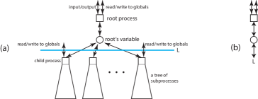
Figure 3: Reduction to a system under hypothesis.

Let us briefly outline this idea. A configuration of a dynamic parametric process is a tree of sub-processes, Figure 3(a). The root performs (1) input/output external operations, (2) read/writes to global variables, and (3) internal operations in form of reads/writes to its local variables, that are also accessible to the child sub-processes. We are now interested in possible sequences of operations on the global variables and the local variables of the root, that can be done by the child sub-processes. If somebody provided us with the set $L_{p}$ of all such possible sequences, for child sub-processes starting at state $p$, for all $p$, we could simplify our system as illustrated in Figure 3(b). We would replace the set of all sub-trees of the root by (a subset of) $L=\{{\sf spawn}(p)\beta:\beta\in\mathsf{pref}(L_{p}),{\sf spawn}(p)\in\Sigma_{\mathit{sp}}\}$ summarizing the possible behaviors of child sub-processes.

A set $L\subseteq\Sigma_{\mathit{sp}}\cdot\Sigma_{\mathit{ext}}^{*}$ is called a hypothesis, as it represents a guess about the possible behaviors of child sub-processes.

Let us now formalize the notion of execution of the system under hypothesis. For that, we define a system $\mathcal{S}_{L}$ that cannot spawn child sub-processes, but instead may use the hypothesis $L$. We will show that if $L$ correctly describes the behavior of child sub-processes then the set of runs of $\mathcal{S}_{L}$ equals the set of runs of $\mathcal{S}$ with child sub-processes. This approach provides a way to compute the set of possible external behaviors of the original process tree level-wise: first for systems restricted to s-trees of height at most $1$, then $2$, …, until a fixpoint is reached.

The configurations of $\mathcal{S}_{L}$ are of the form $(q,\lambda,B)$, where $\lambda$ is as before a valuation of local variables, and $B\subseteq\mathsf{pref}(L)$ is a set of sequences of external actions for sets of sub-processes.

The initial state is $r_{\mathsf{init}}=(q_{\mathsf{init}},\lambda_{\mathsf{init}},\emptyset)$. We will use $r$ to range over configurations of $\mathcal{S}_{L}$. Transitions between two states $r_{1}\stackrel{{\scriptstyle a}}{{\dashrightarrow}}_{L}r_{2}$ are listed in Figure 4. Notice that transitions on actions of child sub-processes are modified so that now $L$ is used to test if an action of a simulated child sub-process is possible.

External transitions under hypothesis:

$$\begin{array}[]{lclll}(q_{1},\lambda,B)&\stackrel{{\scriptstyle a}}{{\dashrightarrow}}_{L}&(q_{2},\lambda,B)&\text{if}&q_{1}\stackrel{{\scriptstyle a}}{{\longrightarrow}}q_{2}\;\text{if $a\in\Sigma_{\mathit{ext}}$}\\ (q,\lambda,B)&\stackrel{{\scriptstyle\overline{\mathit{w}}(g,v)}}{{\dashrightarrow}}_{L}&(q,\lambda,B\cup B^{\prime}\cdot\{\mathit{w}(g,v)\})&\text{if}&\emptyset\neq B^{\prime}\subseteq B,\;B^{\prime}\cdot\{\mathit{w}(g,v)\}\subseteq\mathsf{pref}(L)\\ (q,\lambda,B)&\stackrel{{\scriptstyle\overline{\mathit{r}}(g,v)}}{{\dashrightarrow}}_{L}&(q,\lambda,B\cup B^{\prime}\cdot\{\mathit{r}(g,v)\})&\text{if}&\emptyset\neq B^{\prime}\subseteq B,\;B^{\prime}\cdot\{\mathit{r}(g,v)\}\subseteq\mathsf{pref}(L)\end{array}$$

Internal transitions under hypothesis:

$$\begin{array}[]{lclll}(q_{1},\lambda,B)&\stackrel{{\scriptstyle\tau}}{{\dashrightarrow}}_{L}&(q_{2},\lambda,B)&\text{if}&q_{1}\stackrel{{\scriptstyle\tau}}{{\longrightarrow}}q_{2}\\ (q_{1},\lambda,B)&\stackrel{{\scriptstyle{\sf spawn}(p)}}{{\dashrightarrow}}_{L}&(q_{2},\lambda,B\cup\{{\sf spawn}(p)\})&\text{if}&q_{1}\stackrel{{\scriptstyle{\sf spawn}(p)}}{{\longrightarrow}}q_{2}\;\text{and}\;{\sf spawn}(p)\in\mathsf{pref}(L)\\ (q_{1},\lambda,B)&\stackrel{{\scriptstyle\mathit{w}(x,v)}}{{\dashrightarrow}}_{L}&(q_{2},\lambda^{\prime},B)&\text{if}&q_{1}\stackrel{{\scriptstyle\mathit{w}(x,v)}}{{\longrightarrow}}q_{2}\;\text{and}\;\lambda^{\prime}=\lambda[v/x]\\ (q_{1},\lambda,B)&\stackrel{{\scriptstyle\mathit{r}(x,v)}}{{\dashrightarrow}}_{L}&(q_{2},\lambda,B)&\text{if}&q_{1}\stackrel{{\scriptstyle\mathit{r}(x,v)}}{{\longrightarrow}}q_{2}\;\text{and}\;\lambda(x)=v\\ (q,\lambda,B)&\stackrel{{\scriptstyle\overline{\mathit{w}}(x,v)}}{{\dashrightarrow}}_{L}&(q,\lambda^{\prime},B\cup B^{\prime}\cdot\{\mathit{o}(x,v)\})&\text{if}&\emptyset\neq B^{\prime}\subseteq B,\;B^{\prime}\cdot\{\mathit{o}(x,v)\}\subseteq\mathsf{pref}(L)\\ &&&&\lambda^{\prime}=\lambda[v/x]\\ (q,\lambda,B)&\stackrel{{\scriptstyle\overline{\mathit{r}}(x,v)}}{{\dashrightarrow}}_{L}&(q,\lambda,B\cup B^{\prime}\cdot\{\mathit{i}(x,v)\})&\text{if}&\emptyset\neq B^{\prime}\subseteq B,\;B^{\prime}\cdot\{\mathit{i}(x,v)\}\subseteq\mathsf{pref}(L),\\ &&&&\lambda(x)=v\end{array}$$

Figure 4: Transitions under hypothesis ($g\in G$, $x\in X$).

We list below two properties of $\stackrel{{\scriptstyle}}{{\dashrightarrow}}_{L}$. In order to state them in a convenient way, we introduce a filtering operation $\mathsf{filter}$ on sequences. The point is that external actions of child sub-processes are changed to $\overline{\mathit{r}}$ and $\overline{\mathit{w}}$, when they are exposed at the root of a configuration tree. In the definition below we rename them back; additionally, we remove irrelevant actions. So $\mathsf{filter}(\alpha)$ is obtained by the following renaming of $\alpha$:

$$\mathsf{filter}:\qquad\begin{array}[]{lll}\overline{\mathit{r}}(x,v)\to\mathit{i}(x,v)\,,&&\overline{\mathit{r}}(g,v)\to\mathit{r}(g,v)\,,\\ \overline{\mathit{w}}(x,v)\to\mathit{o}(x,v)\,,&&\overline{\mathit{w}}(g,v)\to\mathit{w}(g,v)\,,\\ a\to a&&\text{if }a\in\Sigma_{\mathit{sp}}\,,\\ a\to\epsilon&&\text{otherwise}\end{array}$$

The next two lemmas follow directly from the definition of $\stackrel{{\scriptstyle\alpha}}{{\dashrightarrow}}_{L}$.

Lemma 3

If $(q,\lambda,\emptyset)\stackrel{{\scriptstyle\alpha}}{{\dashrightarrow}}_{L}(q^{\prime},\lambda^{\prime},B)$ then $B\subseteq\mathsf{pref}(L)$, and every $\beta\in B$ is a scattered subword of $\mathsf{filter}(\alpha)$.

Lemma 4

If $L_{1}\subseteq L_{2}$ and $(p,\lambda,\emptyset)\stackrel{{\scriptstyle\alpha}}{{\dashrightarrow}}_{L_{1}}r$ then $(p,\lambda,\emptyset)\stackrel{{\scriptstyle\alpha}}{{\dashrightarrow}}_{L_{2}}r$.

The next lemma states a basic property of the relation $\stackrel{{\scriptstyle\alpha}}{{\dashrightarrow}}_{L}$. If we take for $L$ the set of all possible behaviors of child sub-processes with s-trees of height at most $k$, then $\stackrel{{\scriptstyle\alpha}}{{\dashrightarrow}}_{L}$ gives us all possible behaviors of a system with s-trees of height at most $k+1$. This corresponds exactly to the situation depicted in Figure 3.

Lemma 5

Suppose $L=\mathit{Ext}_{k}$. For every $p,q$, $\lambda$, and $\alpha$ we have: $(p,\lambda_{\mathsf{init}},\emptyset)\stackrel{{\scriptstyle\alpha}}{{\dashrightarrow}}_{L}(q,\lambda,B)$ for some $B$ iff $(p,\lambda_{\mathsf{init}},\emptyset)\stackrel{{\scriptstyle\alpha}}{{\Longrightarrow}}_{k+1}(q,\lambda,S)$ for some $S$.

Proof.

The statement may look almost tautological, but is not. We prove two directions:

1. Whenever $(p,\lambda_{\mathsf{init}},\emptyset)\stackrel{{\scriptstyle\alpha}}{{\Longrightarrow}}_{k+1}(q,\lambda,S)$, then there is some $B$ so that $(p,\lambda_{\mathsf{init}},\emptyset)\stackrel{{\scriptstyle\alpha}}{{\dashrightarrow}}_{L}(q,\lambda,B)$ holds.

2. Whenever $(p,\lambda_{\mathsf{init}},\emptyset)\stackrel{{\scriptstyle\alpha}}{{\dashrightarrow}}_{L}(q,\lambda,B)$, then there is some finite set $S$ of s-trees of depth at most $k$ so that $(p,\lambda_{\mathsf{init}},\emptyset)\stackrel{{\scriptstyle\alpha}}{{\Longrightarrow}}_{k+1}(q,\lambda,S)$.

Statement 1 follows by induction on the length of $\alpha$ where the set $B$ satisfies the invariant that for every $s\in S$, there is some $\beta={\sf spawn}(p^{\prime})\beta^{\prime}$ in $B$ such that $(p^{\prime},\lambda_{\mathsf{init}},\emptyset)\stackrel{{\scriptstyle\alpha^{\prime}}}{{\Longrightarrow}}_{k}s$ holds for some $\alpha^{\prime}$, with $\mathit{ext}(\alpha^{\prime})=\beta^{\prime}$.

The proof of statement 2 is more technical. Assume that $\alpha=a_{1}\cdots a_{n}$ and $(p_{i},\lambda_{i},B_{i})\stackrel{{\scriptstyle a_{i}}}{{\dashrightarrow}}_{L}(p_{i+1},\lambda_{i+1},B_{i+1})$ for $i=1,\ldots,n$, where $(p_{1},\lambda_{1},B_{1})=(p,\lambda_{\mathsf{init}},\emptyset)$ and $(p_{n+1},\lambda_{n+1},B_{n+1})=(q,\lambda,B)$. We construct below a corresponding sequence of sets of $s$-trees $S_{1},\ldots,S_{n+1}$ with $(p_{i},\lambda_{i},S_{i})\stackrel{{\scriptstyle a_{i}}}{{\Longrightarrow}}_{k}(p_{i+1},\lambda_{i+1},S_{i+1})$, $i=1,\ldots,n$.

Since $B_{n+1}\subseteq\mathsf{pref}(\mathit{Ext}_{k})$, we have for every $\beta={\sf spawn}(p_{\beta})\beta^{\prime}\in B_{n+1}$ that $(p_{\beta},\lambda_{\mathsf{init}},\emptyset)\stackrel{{\scriptstyle\gamma_{\beta}}}{{\Longrightarrow}}_{k}(q_{\beta},\lambda,S_{\beta})$, for some $\gamma_{\beta}$ with $\mathit{ext}(\gamma_{\beta})=\beta^{\prime}$. This means for $\beta^{\prime}=b_{\beta,1}\cdots b_{\beta,n_{\beta}}$ that $\gamma_{\beta}$ has the form: $\gamma_{\beta}=\gamma_{\beta,1}b_{\beta,1}\cdots\gamma_{\beta,n_{\beta}}b_{\beta,n_{\beta}}$ with $\mathit{ext}(\gamma_{\beta,j})=\varepsilon$ for all $j$. Moreover, there are s-trees $s_{\beta,j}$ of depth at most $k$ so that $s_{\beta,j}\stackrel{{\scriptstyle\gamma_{\beta,j}b_{\beta,j}}}{{\Longrightarrow}}_{k}s_{\beta,j+1}$ for $j=1,\ldots,n_{\beta}$ with $s_{\beta,1}=(p_{\beta},\lambda_{\mathsf{init}},\emptyset)$ and $s_{\beta,n_{\beta}+1}=(q_{\beta},\lambda,S_{\beta})$. Then we define $S_{i}$ as the set of all $s_{\beta,j}$ such that ${\sf spawn}(p_{\beta})b_{\beta,1}\cdots b_{\beta,j-1}$ is a scattered subword of $\mathsf{filter}(a_{1}\cdots a_{i-1})$.

It remains to prove that $(p_{i},\lambda_{i},S_{i})\stackrel{{\scriptstyle a_{i}}}{{\Longrightarrow}}_{k}(p_{i+1},\lambda_{i+1},S_{i+1})$ holds for every $i=1,\ldots,n$. For that we perform a case distinction on action $a_{i}$. If $a_{i}$ is of the form $\tau,\mathit{r}(g,v),\mathit{w}(g,v),\mathit{i}(x,v)$ or $\mathit{o}(x,v)$, then $B_{i+1}=B_{i}$, $S_{i+1}=S_{i}$ and the assertion holds. If $a_{i}$ is the action ${\sf spawn}(p^{\prime})$, then $B_{i+1}=B_{i}\cup\{{\sf spawn}(p^{\prime})\}$. Likewise, $S_{i+1}=S_{i}\cup\{(p^{\prime},\lambda_{\mathsf{init}},\emptyset)\}$ in accordance with our claim.

The most complicated case is when $a_{i}$ is of one of the forms $\overline{\mathit{r}}(y,v),\overline{\mathit{w}}(y,v)$ for $y\in X\cup G$ and $v\in V$. Then $B_{i+1}=B_{i}\cup B^{\prime}\cdot\{b\}$ for $b=\mathsf{filter}(a_{i})$ and some $B^{\prime}\subseteq B_{i}$ with $B^{\prime}\cdot\{b_{i}\}\subseteq B_{n+1}\subseteq\mathsf{pref}(L)$. Let $S$ be the set consisting of all $s_{\beta,j+1}$ such that ${\sf spawn}(p_{\beta})b_{\beta,1}\cdots b_{\beta,j}$ is a scattered subword of $\mathsf{filter}(a_{1}\dots a_{i})$ and $b_{\beta,j}=b$. This set $S$ is not empty since $B^{\prime}$ is not empty. We have $S_{i+1}=S_{i}\cup S$ by the definition of $S_{i}$ and $S_{i+1}$. Now for every $s_{\beta,j+1}\in S$ we have by definition $s_{\beta,j}\stackrel{{\scriptstyle\gamma_{\beta,j}b_{\beta,j}}}{{\Longrightarrow}}_{k}s_{\beta,j+1}$, and $b_{\beta,j}=b$. Since ${\sf spawn}(p_{\beta})b_{\beta,1}\cdots b_{\beta,j-1}$ is a scattered subword of $\mathsf{filter}(a_{1}\cdots a_{i-1})$, we have $s_{\beta,j}\in S_{i}$. This shows that we have indeed $(p_{i},\lambda_{i},S_{i})\stackrel{{\scriptstyle a_{i}}}{{\Longrightarrow}}_{k}(p_{i+1},\lambda_{i+1},S_{i}\cup S)$, with $S_{i}\cup S=S_{i+1}$.

∎∎

The question we will pursue now is whether in the lemma above, we may replace $\mathit{Ext}_{k}$ with some simpler set and still get all computations of the system of height $k+1$. Of central importance here is the following lemma saying that the lift operation (cf. Definition 5) does not add new behaviours.

Lemma 6

Assume that $L\subseteq\Sigma_{\mathit{sp}}\cdot\Sigma_{\mathit{ext}}^{*}$ and $L^{\prime}=\mathsf{lift}(L)$. Then $(p,\lambda_{\mathsf{init}},\emptyset)\stackrel{{\scriptstyle\alpha}}{{\dashrightarrow}}_{L}(q,\lambda,B)$ for some $B\subseteq\mathsf{pref}(L)$ iff $(p,\lambda_{\mathsf{init}},\emptyset)\stackrel{{\scriptstyle\alpha}}{{\dashrightarrow}}_{L^{\prime}}(q,\lambda,B^{\prime})$ for some $B^{\prime}\subseteq\mathsf{pref}(L^{\prime})$.

Proof.

The left-to-right direction is obvious by monotonicity, since $L\subseteq L^{\prime}$.

We focus on the right-to-left direction. The main idea is that the first occurrences of actions in sequences from $B$ suffice to simulate any sequence from $B^{\prime}$.

Assume that $\alpha=a_{1}\cdots a_{n}$, and $(p_{i},\lambda_{i},B^{\prime}_{i})\stackrel{{\scriptstyle a_{i}}}{{\dashrightarrow}}_{L^{\prime}}(p_{i+1},\lambda_{i+1},B^{\prime}_{i+1})$ for $i=1,\ldots,n$ where $(p_{1},\lambda_{1},B^{\prime}_{1})=(p,\lambda_{\mathsf{init}},\emptyset)$ and $(p_{n+1},\lambda_{n+1},B^{\prime}_{n+1})=(q,\lambda,B^{\prime})$. For $i=1,\ldots,n+1$, we define a subset $B_{i}\subseteq\mathsf{pref}(L)$ by $B_{i}=\{\beta\in\mathsf{pref}(L):\mathsf{lift}(\beta)\cap B^{\prime}_{i}\neq\emptyset\}$. By case distinction, we verify that indeed $(p_{i},\lambda_{i},B_{i})\stackrel{{\scriptstyle a_{i}}}{{\dashrightarrow}}_{L}(p_{i+1},\lambda_{i+1},B_{i+1})$ holds for $i=1,\ldots,n$. If $a_{i}$ is either $\tau,\mathit{r}(x,v),\mathit{w}(x,v)$ or in $\Sigma_{\mathit{ext}}$, then $B^{\prime}_{i+1}=B^{\prime}_{i}$, $B_{i+1}=B_{i}$, and the assertion holds inductively. If $a_{i}$ is the action ${\sf spawn}(p^{\prime})$, then $B^{\prime}_{i+1}=B^{\prime}_{i}\cup\{{\sf spawn}(p^{\prime})\}$, $B_{i+1}=B_{i}\cup\{{\sf spawn}(p^{\prime})\}$, and the assertion holds, again by induction.

It remains to consider the case where $a_{i}$ is $\overline{\mathit{r}}(y,v)$ or $\overline{\mathit{w}}(y,v)$, where $y\in X\cup G$, $v\in V$. Let $b=\mathsf{filter}(a_{i})$, and $B^{\prime}_{i+1}=B^{\prime}_{i}\cup B^{\prime}\cdot\{b\}$ for some $\emptyset\neq B^{\prime}\subseteq B^{\prime}_{i}$ with $B^{\prime}\cdot\{b\}\subseteq\mathsf{pref}(L^{\prime})$. We need to find some $B\subseteq B_{i}$ such that $B_{i+1}=B_{i}\cup B\cdot\{b\}$.

Let $B=\{\beta\in B_{i}:\mathsf{lift}(\beta)\cap B^{\prime}\not=\emptyset\}$. We claim that $B_{i}\cup B\cdot\{b\}=B_{i+1}$. To show $B_{i}\cup B\cdot\{b\}\subseteq B_{i+1}$ we argue that for every $\beta\in B$, $\mathsf{lift}(\beta b)\cap B^{\prime}b\not=\emptyset$. Conversely, let $\beta^{\prime}b\in B^{\prime}\{b\}$, and $\beta\in B_{i+1}$ such that $\beta^{\prime}b\in\mathsf{lift}(\beta)$. We need to show that $\beta\in B_{i}\cup B\{b\}$. In particular, we know that $\beta\in\mathsf{pref}(L)$. Either $\beta$ is of the form $\beta=\beta_{1}b$ and $\beta_{1}$ has no $b$. Thus, $\beta^{\prime}\in\mathsf{lift}(\beta_{1})$, so $\beta_{1}\in B$ and $\beta\in B\{b\}$. Or $\beta=\beta_{1}b\beta_{2}$ with $\beta^{\prime}\in\mathsf{lift}(\beta)$. Since $\beta^{\prime}\in B^{\prime}_{i}$ we have in this case $\beta\in B_{i}$ by definition.∎

∎

So Lemma 5 says that child sub-processes can be abstracted by their external behaviors. Lemmas 4 and 6 allow to abstract a set $L$ of external behaviors by a subset $L_{1}\subseteq L$, as long as $L\subseteq\mathsf{lift}(L_{1})$ holds. In the following, we introduce a well-quasi-order to characterize a smallest such subset, which we call core.

Definition 6 (Order, core)

We define an order on $\Sigma_{\mathit{ext}}^{*}$ by $\alpha\preccurlyeq\beta$ if $\beta\in\mathsf{lift}(\alpha)$. This extends to an order on $\Sigma_{\mathit{sp}}\cdot\Sigma_{\mathit{ext}}^{*}$: ${\sf spawn}(p)\alpha\preccurlyeq{\sf spawn}(q)\beta$ if $p=q$ and $\alpha\preccurlyeq\beta$. For a set $L\subseteq\Sigma_{\mathit{sp}}\cdot\Sigma_{\mathit{ext}}^{*}$, we define $\operatorname{\textsf{core}}(L)$ as the set of minimal words in $L$ with respect to the relation $\preccurlyeq$.

The following lemma states the most important property of the order $\preccurlyeq$:

Lemma 7

The relation $\preccurlyeq$ is a well-quasi-order on words with equal signature. Since the number of signatures is finite, the set $\operatorname{\textsf{core}}(L)$ is finite for every set $L\subseteq\Sigma_{\mathit{sp}}\cdot\Sigma_{\mathit{ext}}^{*}$.

Proof.

We spell out what it means that $\alpha\preccurlyeq\beta$, by expanding the definition of $\mathsf{lift}(\alpha)$. First recall that if $\alpha\preccurlyeq\beta$ then the two sequences have the same signatures. Let $\alpha={\sf spawn}(p)\alpha^{\prime}$ and $\beta={\sf spawn}(p)\beta^{\prime}$, $\mathsf{sig}(\alpha^{\prime})=\mathsf{sig}(\beta^{\prime})=b_{1}\cdots b_{k}$ for some $p$. Consider the canonical decompositions of $\alpha^{\prime},\beta^{\prime}$:

$$\alpha^{\prime}=b_{1}\alpha^{\prime}_{1}b_{2}\alpha^{\prime}_{2}\cdots b_{k}\alpha_{k}\,,\qquad\beta^{\prime}=b_{1}\beta^{\prime}_{1}b_{2}\beta^{\prime}_{2}\cdots b_{k}\beta_{k}\ .$$

We have $\alpha\preccurlyeq\beta$ iff $\alpha^{\prime}_{i}$ is a scattered subword of $\beta^{\prime}_{i}$, for every $i=1,\dots,k+1$. Since being a scattered subword is a well-quasi-order relation, the lemma follows. ∎∎

Consider, e.g., the set $L=\mathit{Ext}_{1}$ of all external behaviors of depth 1 in Example 1. Then $\operatorname{\textsf{core}}(L)$ consists of the sequences:

$${\sf spawn}(q)\,\mathit{w}(g_{0},\#),\;{\sf spawn}(p)\,\mathit{i}(x,1)\mathit{o}(x,2)\mathit{o}(x,3),\;{\sf spawn}(p)\,\mathit{i}(x,1)\mathit{o}(x,3)\mathit{o}(x,2)$$

together with all their prefixes (recall that $k$ in $\mathit{Ext}_{k}$ refers to s-trees of depth at most $k$).

The development till now can be summarized by the following:

Corollary 2

For a set $L\subseteq\Sigma_{\mathit{sp}}\cdot\Sigma_{\mathit{ext}}^{*}$, and $L^{\prime}=\operatorname{\textsf{core}}(L)$: $(p,\lambda_{\mathsf{init}},\emptyset)\stackrel{{\scriptstyle\alpha}}{{\dashrightarrow}}_{L}(q,\lambda,B)$ for some $B\subseteq L$ iff $(p,\lambda_{\mathsf{init}},\emptyset)\stackrel{{\scriptstyle\alpha}}{{\dashrightarrow}}_{L^{\prime}}(q,\lambda,B^{\prime})$ for some $B^{\prime}\subseteq L^{\prime}$.

Proof.

Since $\operatorname{\textsf{core}}(L)\subseteq L$, the right-to-left implication follows by monotonicity. For the other direction we observe that $L\subseteq\mathsf{lift}(\operatorname{\textsf{core}}(L))$, so we can use Lemma 6 and monotonicity. ∎∎

Now we turn to the question of computing the relation $\stackrel{{\scriptstyle\alpha}}{{\dashrightarrow}}_{L}$ for a finite set $L$. For this we need our admissibility assumptions from page 3.

Proposition 2

Let $\mathcal{C}$ be an admissible class of automata, and let $\mathcal{S}$ be a transition system whose associated automaton is in $\mathcal{C}$. Suppose we have two sets $L,L^{\prime}\subseteq\Sigma_{\mathit{sp}}\cdot\Sigma_{\mathit{ext}}^{*}$ with $L\subseteq L^{\prime}\subseteq\mathsf{lift}(L)$. Consider the set

$$K=\{{\sf spawn}(p)\mathit{ext}(\alpha):{\sf spawn}(p)\in\Sigma_{\mathit{sp}}\text{ and }(p,\lambda_{\mathsf{init}},\emptyset)\stackrel{{\scriptstyle\alpha}}{{\dashrightarrow}}_{L^{\prime}}r^{\prime},\text{for some $r^{\prime}$}\}$$

determined by $\mathcal{S}$ and $L^{\prime}$. If $L$ is finite then we can compute the sets

$$\operatorname{\textsf{core}}(K)\quad\text{and}\quad\operatorname{\textsf{core}}(\{\alpha\in K:\text{$\alpha$ consistent}\})\ .$$

The proof of the above proposition works by augmenting the transition system $\mathcal{S}$ by a finite-state component taking care of the valuation of local variables and of prefixes of $L$ that were used in the hypothesis. The admissibility of $\mathcal{C}$ is then used to compute the core of the language of the automaton thus obtained.

Proof.

By Lemmas 4 and 6, the relations $\stackrel{{\scriptstyle\alpha}}{{\dashrightarrow}}_{L}$ and $\stackrel{{\scriptstyle\alpha}}{{\dashrightarrow}}_{L^{\prime}}$ are the same. Since $L$ is finite, there are only finitely many sets $B\subseteq L$. Moreover, the number of valuations $\lambda$ is finite by our initial definitions. This allows to construct a finite automaton $\mathcal{A}$, whose states are pairs $(\lambda,B)$ and transitions are as those of $\stackrel{{\scriptstyle}}{{\dashrightarrow}}_{L}$ but without the first component:

$$\begin{array}[]{lclll}(\lambda,B)&\stackrel{{\scriptstyle\overline{\mathit{w}}(g,v)}}{{\longrightarrow}}&(\lambda,B\cup B^{\prime}\cdot\{\mathit{w}(g,v)\})&\text{if}&\emptyset\neq B^{\prime}\subseteq B,\;B^{\prime}\cdot\{\mathit{w}(g,v)\}\subseteq\mathsf{pref}(L),\\ (\lambda,B)&\stackrel{{\scriptstyle\overline{\mathit{r}}(g,v)}}{{\longrightarrow}}&(\lambda,B\cup B^{\prime}\cdot\{\mathit{r}(g,v)\})&\text{if}&\emptyset\neq B^{\prime}\subseteq B,\;B^{\prime}\cdot\{\mathit{r}(g,v)\}\subseteq\mathsf{pref}(L)\end{array}$$

$$\begin{array}[]{lclll}(\lambda,B)&\stackrel{{\scriptstyle{\sf spawn}(p)}}{{\longrightarrow}}&(\lambda,B\cup\{{\sf spawn}(p)\})&\text{if ${\sf spawn}(p)\in\mathsf{pref}(L)$}\\ (\lambda,B)&\stackrel{{\scriptstyle\mathit{w}(x,v)}}{{\longrightarrow}}&(\lambda[v/x],B)\\ (\lambda,B)&\stackrel{{\scriptstyle\mathit{r}(x,v)}}{{\longrightarrow}}&(\lambda,B)&\text{if $\lambda(x)=v$}\\ (\lambda,B)&\stackrel{{\scriptstyle\overline{\mathit{w}}(x,v)}}{{\longrightarrow}}&(\lambda[v/x],B\cup B^{\prime}\cdot\{\mathit{o}(x,v)\})&\text{if }\emptyset\neq B^{\prime}\subseteq B,\;B^{\prime}\cdot\{\mathit{o}(x,v)\}\subseteq\mathsf{pref}(L)\\ (\lambda,B)&\stackrel{{\scriptstyle\overline{\mathit{r}}(x,v)}}{{\longrightarrow}}&(\lambda,B\cup B^{\prime}\cdot\{\mathit{i}(x,v)\})&\text{if }\lambda(x)=v,\,\emptyset\neq B^{\prime}\subseteq B,\;B^{\prime}\cdot\{\mathit{i}(x,v)\}\subseteq\mathsf{pref}(L)\\ (\lambda,B)&\stackrel{{\scriptstyle a}}{{\longrightarrow}}&(\lambda,B)&\text{for all }a\in\Sigma_{\mathit{ext}}\end{array}$$

Now consider the automaton $\mathcal{A}_{\mathcal{S}}$ associated to $\mathcal{S}$. This automaton belongs to our admissible class $\mathcal{C}$, so its alphabet extension is also in $\mathcal{C}$:

$$\mathcal{A}^{\prime}_{\mathcal{S}}=\mathcal{A}_{\mathcal{S}}\!\circlearrowleft\!\{\overline{\mathit{r}}(y,v),\overline{\mathit{w}}(y,v):y\in X\cup G,v\in V\}\ .$$

Intuitively, we add to $\mathcal{A}_{\mathcal{S}}$ self-loops on actions that are in $\mathcal{A}_{L}$ but not in $\mathcal{A}_{\mathcal{S}}$. Finally, consider the product $\mathcal{A}^{K}=\mathcal{A}^{\prime}_{\mathcal{S}}\times\mathcal{A}_{L}$. We have that for every pair of states $q,q^{\prime}$, valuations $\lambda,\lambda^{\prime}$, and sets $B,B^{\prime}$: $(q,\lambda,B)\stackrel{{\scriptstyle\alpha}}{{\dashrightarrow}}_{L}(q^{\prime},\lambda,B^{\prime})$ iff there is a path labeled $\alpha$ from $(q,\lambda,B)$ to $(q^{\prime},\lambda,B^{\prime})$ in $\mathcal{A}^{K}$. Then ${\sf spawn}(p)\alpha\in K$ iff there is path in $\mathcal{A}^{K}$ from $(p,\lambda_{\mathsf{init}},\emptyset)$ labeled by some $\alpha^{\prime}$ with $\mathit{ext}(\alpha^{\prime})=\alpha$.

The above paragraph says that in order to compute $\operatorname{\textsf{core}}(K)$ it is enough to compute $\operatorname{\textsf{core}}(\mathit{ext}(K_{p}))$ where $K_{p}$ is the set of labels of runs of $\mathcal{A}^{K}$ from $(p,\lambda_{\mathsf{init}},\emptyset)$. Since $\mathcal{A}^{K}$ belongs to our admissible class $\mathcal{C}$, we can use the effective emptiness test. If the language of $\mathcal{A}^{K}$ is not empty then we can find a word $\alpha_{1}$ that is accepted from $(p,\lambda_{\mathsf{init}},\emptyset)$. Next we look for $\beta\in\operatorname{\textsf{core}}(\mathit{ext}(K_{p}))$ with $\beta\preccurlyeq\mathit{ext}(\alpha_{1})$. To this end, for every $\beta\preccurlyeq\mathit{ext}(\alpha_{1})$ we consider an automaton $\mathcal{A}^{\beta}$ accepting all the words $\alpha^{\prime}$ such that $\mathit{ext}(\alpha^{\prime})=\beta$. We build the product of $\mathcal{A}^{K}$ with $\mathcal{A}^{\beta}$ and check for emptiness. Then we choose one minimal $\beta_{1}$ for which this product is non-empty.

To find a next word from $\operatorname{\textsf{core}}(ext(K_{p}))$ we construct a finite automaton $\mathcal{N}_{\beta_{1}}$ accepting all words $\alpha^{\prime}$ such that $\beta_{1}\not\preccurlyeq\mathit{ext}(\alpha^{\prime})$. Then we consider $\mathcal{A}^{K}\times\mathcal{N}_{\beta_{1}}$ instead of $\mathcal{A}^{K}$. If the language accepted by $\mathcal{A}^{K}\times\mathcal{N}_{\beta_{1}}$ is not empty then we get a word $\alpha_{2}$ in the language. We apply the above procedure to $\alpha_{2}$, iterating through all words $\beta\preccurlyeq\mathit{ext}(\alpha_{2})$ and checking if the language of $\mathcal{A}^{K}\times\mathcal{A}^{\beta}_{\beta_{1}}$ is empty; here $\mathcal{A}^{\beta}_{\beta_{1}}$ is a finite automaton accepting all words $\alpha^{\prime}$ such that $\mathit{ext}(\alpha^{\prime})=\beta$ and $\alpha^{\prime}\in\mathcal{N}_{\beta_{1}}$. We choose one minimal $\beta_{2}$ for which such a product is non-empty. For the following iteration we construct $\mathcal{N}_{\beta_{2}}$ accepting all words $\alpha^{\prime}$ such that $\beta_{2}\not\preccurlyeq\mathit{ext}(\alpha^{\prime})$. So $\mathcal{N}_{\beta_{1}}\times\mathcal{N}_{\beta_{2}}$ accepts all words $\alpha^{\prime}$ that $\beta_{1}\not\preccurlyeq\mathit{ext}(\alpha^{\prime})$ and $\beta_{2}\not\preccurlyeq\mathit{ext}(\alpha^{\prime})$. We continue this way, finding words $\beta_{1},\dots,\beta_{k}\in\operatorname{\textsf{core}}(\mathit{ext}(K_{p}))$ till $\mathcal{A}^{K}\times\mathcal{N}_{\beta_{1}}\times\dots\times\mathcal{N}_{\beta_{k}}$ is empty. At that point we know that $\{\beta_{1},\dots,\beta_{k}\}=\operatorname{\textsf{core}}(\mathit{ext}(K_{p}))$.

This procedure works also for the second statement by observing that the set of all consistent sequences, let us call it $\mathit{Consistent}$, is a regular language. So instead of starting with $K$ in the above argument we start with $K\cap\mathit{Consistent}$. ∎

∎

In the next two corollaries, $\mathcal{S}$ is such that its associated automaton $\mathcal{A}_{\mathcal{S}}$ belongs to an admissible class.

Corollary 3

The sets $\operatorname{\textsf{core}}(\mathit{Ext}_{0})$ and $\operatorname{\textsf{core}}(\mathit{Ext}_{0}\cap\mathit{Consistent})$ are computable.

Proof.

As we are concerned with s-trees of depth 0, all occurring configurations are of the form $(q,\lambda,\emptyset)$. This means that ${\sf spawn}(p)\alpha\in\mathit{Ext}_{0}$ iff $(p,\lambda_{\mathsf{init}},\emptyset)\stackrel{{\scriptstyle\alpha}}{{\dashrightarrow}}_{\emptyset}(q,\lambda,\emptyset)$ for some $q$ and $\lambda$. We can then use Proposition 2 with $L=L^{\prime}=\emptyset$. ∎∎

Corollary 4

Under the hypothesis of Proposition 2: for every $k\geq 0$, we can compute $\operatorname{\textsf{core}}(\mathit{Ext}_{k})$ and $\operatorname{\textsf{core}}(\mathit{Ext}_{k}\cap\mathit{Consistent})$.

Proof.

We start with $L_{0}=\operatorname{\textsf{core}}(\mathit{Ext}_{0})$ that we can compute by Corollary 3. Now assume that $L_{i}=\operatorname{\textsf{core}}(\mathit{Ext}_{i})$ has already been computed. By Lemma 5, $L_{i+1}$ equals the core of $\{{\sf spawn}(p)\mathit{ext}(\alpha):(p,\lambda_{\mathsf{init}},\emptyset)\stackrel{{\scriptstyle\alpha}}{{\dashrightarrow}}_{L_{i}}r,\;\text{some $r$}\}$ which, by Proposition 2, is effectively computable. ∎∎

Now we have all ingredients to prove Theorem 2.1.

of Theorem 2.1.

Take a process $\mathcal{S}$ as in the statement of the theorem. The external behaviors of $\mathcal{S}$ are described by the language

$$L=\bigcup_{k\in\mathbb{N}}\{{\sf spawn}(p)\mathit{ext}(\alpha):(p,\lambda_{\mathsf{init}},\emptyset)\stackrel{{\scriptstyle\alpha}}{{\dashrightarrow}}_{\mathit{Ext}_{k}}r,\text{ for some }r\}$$

If we denote $L_{k}=\operatorname{\textsf{core}}(\mathit{Ext}_{k})$ then by Corollary 2, the language $L$ is equal to

$$L^{\prime}=\bigcup_{k\in\mathbb{N}}\{{\sf spawn}(p)\mathit{ext}(\alpha):(p,\lambda_{\mathsf{init}},\emptyset)\stackrel{{\scriptstyle\alpha}}{{\dashrightarrow}}_{L_{k}}r,\text{ for some }r\}$$

By definition, $\mathit{Ext}_{0}\subseteq\mathit{Ext}_{1}\subseteq\cdots$ is an increasing sequence of sets. By Lemma 7, this means that there is some $m$ so that $\operatorname{\textsf{core}}(\mathit{Ext}_{m})=\operatorname{\textsf{core}}(\mathit{Ext}_{m+i})$, for all $i$. Therefore, $L^{\prime}$ is equal to

$$\{{\sf spawn}(p)\mathit{ext}(\alpha):(p,\lambda_{\mathsf{init}},\emptyset)\stackrel{{\scriptstyle\alpha}}{{\dashrightarrow}}_{L_{m}}r,\text{ for some }r\}$$

By Corollary 4, the set $L_{m}=\operatorname{\textsf{core}}(\mathit{Ext}_{m})$ is computable and so is $\operatorname{\textsf{core}}(L^{\prime}\cap\mathit{Consistent})$. Finally, we check if in this latter set there is a sequence starting with ${\sf spawn}(q_{\mathsf{init}})$ and an external write or an output of $\#$.∎∎

6 Processes with generalized features

In this section we consider pushdown dynamic parametric processes where a sub-process cannot write to its own variables, but only to the variables of its parent. This corresponds to the situation when after a parent has created sub-processes, the latter may communicate computed results to the parent and to their siblings, but the parent cannot communicate to child sub-processes. We call such a model a pushdown dynamic parametric process with generalized futures. We have seen an example of such a system in Figure 1. Technically, processes with generalized futures are obtained by disallowing $\mathit{w}(x,v)$ actions in our general definition. Additionally, we rule out global variables, i.e., $G=\emptyset$. Accordingly, we may no longer define reachability via reachability of a write action to some global variable, but as reachability of an output action $\mathit{o}(x,\#)$ of some special value $\#$ to some variable $x$ of the root process.

For processes with generalized futures, reachability can be decided by a somewhat simpler approach. In particular, we present an Exptime algorithm to decide reachability.

In this section we need an additional assumption concerning the initial value of variables. Since this initial value causes problems as it is the one that cannot be reproduced once overwritten, we require:

Proviso: We consider systems where the initial value $v_{\mathsf{init}}$ of a variable can be neither read nor written.

Since in the case that we consider in this section there are no global variables, the external alphabet simplifies to:

$$\Sigma_{\mathit{ext}}=\{\mathit{i}(x,v),\mathit{o}(x,v):x\in X,v\in V\}\,.$$

From the definition of transitions $r_{1}\stackrel{{\scriptstyle a}}{{\dashrightarrow}}_{L}r_{2}$ of sub-processes modulo hypothesis we can see that the label $a$ can be either an external action, or internal action of the form: $\tau,{\sf spawn}(p),\mathit{r}(x,v),\overline{\mathit{w}}(x,v),\overline{\mathit{r}}(x,v)$.

Disallowing $\mathit{w}(x,v)$ operations has an important impact on the $\stackrel{{\scriptstyle\alpha}}{{\dashrightarrow}}_{L}$ semantics. By inspecting the rules, we notice that there is only one remaining rule, namely $\overline{\mathit{w}}(x,v)$, that changes the value of the component $\lambda$, and this rule does not change the state component.

The next lemma is the main technical step in this section. It says that for processes with generalized futures, $\mathsf{sig}(\mathit{Ext}_{k})$ as hypothesis yields the same behaviors as $\mathit{Ext}_{k}$.

Lemma 8

For a dynamic parametric process $\mathcal{S}$ with generalized futures, let $L=\mathsf{sig}(\mathit{Ext}_{k})$ and $L^{\prime}=\mathit{Ext}_{k}$. We have: $(p,\lambda_{\mathsf{init}},\emptyset)\stackrel{{\scriptstyle\alpha}}{{\dashrightarrow}}_{L}(q,\lambda,B)$ for some $\lambda$, $B\subseteq L$ iff $(p,\lambda_{\mathsf{init}},\emptyset)\stackrel{{\scriptstyle\alpha^{\prime}}}{{\dashrightarrow}}_{L^{\prime}}(q,\lambda^{\prime},B^{\prime})$ for some $\lambda^{\prime}$, $B^{\prime}\subseteq L^{\prime}$, and some $\alpha^{\prime}$ with $\mathit{ext}(\alpha)=\mathit{ext}(\alpha^{\prime})$.

Proof.

For the right-to-left implication observe that $\mathit{Ext}_{k}\subseteq\mathsf{lift}(\mathsf{sig}(\mathit{Ext}_{k}))$. So, if $(p,\lambda_{\mathsf{init}},\emptyset)\stackrel{{\scriptstyle\alpha}}{{\dashrightarrow}}_{L^{\prime}}(q,\lambda,B)$ then $(p,\lambda_{\mathsf{init}},\emptyset)\stackrel{{\scriptstyle\alpha}}{{\dashrightarrow}}_{L^{\prime\prime}}(q,\lambda,B)$ for $L^{\prime\prime}=\mathsf{lift}(\mathsf{sig}(\mathit{Ext}_{k}))$. But then Lemma 6 gives us $(p,\lambda_{\mathsf{init}},\emptyset)\stackrel{{\scriptstyle\alpha}}{{\dashrightarrow}}_{L}(q,\lambda,B^{\prime})$ for some $B^{\prime}$.

For the left-to-right implication note first that it does not follow from monotonicity, since $\mathsf{sig}(\mathit{Ext}_{k})$ may contain sequences that are not in $\mathit{Ext}_{k}$. So assume that $\alpha=a_{1}\cdots a_{n}$, and $(p_{i},\lambda_{i},B_{i})\stackrel{{\scriptstyle a_{i}}}{{\dashrightarrow}}_{L}(p_{i+1},\lambda_{i+1},B_{i+1})$ for $i=1,\ldots,n$ where $(p_{1},\lambda_{1},B_{1})=(p,\lambda_{\mathsf{init}},\emptyset)$ and $(p_{n+1},\lambda_{n+1},B_{n+1})=(q,\lambda,B)$. We look for subsets $B^{\prime}_{i}$ of $\mathit{Ext}_{k}$, for $i=1,\dots,n+1$, such that $(p_{i},\lambda^{\prime}_{i},B^{\prime}_{i})\stackrel{{\scriptstyle\delta_{i}a_{i}}}{{\dashrightarrow}}_{L^{\prime}}(p_{i+1},\lambda^{\prime}_{i+1},B^{\prime}_{i+1})$ for some sequence $\delta_{i}$ of internal actions. The additional $\delta$’s are needed since the elements of $L$ are subsequences of those from $L^{\prime}$.

For every maximal signature $\beta\in B_{n+1}\subseteq\mathsf{pref}(L)$, we fix a sequence $\beta^{\prime}\in\mathsf{pref}(L^{\prime})$ such that $\mathsf{sig}(\beta^{\prime})=\beta$: for $\beta={\sf spawn}(p_{\beta})b_{\beta,1}\cdots b_{\beta,n_{\beta}}$ we will write $\beta^{\prime}={\sf spawn}(p_{\beta})b_{\beta,1}\gamma_{\beta,1}\cdots b_{\beta,n_{\beta}}\gamma_{\beta,n_{\beta}}$, for some $\gamma_{\beta,j}\in\Sigma_{\mathit{ext}}^{*}$.

We define $B^{\prime}_{i}$ as the smallest prefix closed set that satisfies the following property for every maximal sequence $\beta\in B_{n+1}$: if the prefix ${\sf spawn}(\beta)b_{\beta,1}\cdots b_{\beta,j}$ is in $B_{i}$ (for some $j\leq n_{\beta}$) then ${\sf spawn}(p_{\beta})b_{\beta,1}\gamma_{\beta,2}\cdots b_{\beta,j-1}\gamma_{\beta,j-1}b_{\beta,j}$ is in $B^{\prime}_{i}$.

It remains to prove that $(p_{i},\lambda^{\prime}_{i},B^{\prime}_{i})\stackrel{{\scriptstyle\delta_{i}a_{i}}}{{\dashrightarrow}}_{L^{\prime}}(p_{i+1},\lambda^{\prime}_{i+1},B^{\prime}_{i+1})$ for some sequence $\delta_{i}$ of internal actions. For that we perform a case distinction on the action $a_{i}$. If $a_{i}$ is $\tau$, $\mathit{i}(x,v)$ or $\mathit{o}(x,v)$, then only the state changes, so the assertion holds by induction. If $a_{i}$ is ${\sf spawn}(p^{\prime})$, then $B_{i+1}=B_{i}\cup\{{\sf spawn}(p^{\prime})\}$. Likewise, $B^{\prime}_{i+1}=B^{\prime}_{i}\cup\{{\sf spawn}(p^{\prime})\}$ according to our claim.

The case $a_{i}=\mathit{r}(x,v)$ is a bit more tricky. If $\lambda^{\prime}_{i}(x)=v$ then we can do $(p_{i},\lambda^{\prime}_{i},B^{\prime}_{i})\stackrel{{\scriptstyle a_{i}}}{{\dashrightarrow}}_{L^{\prime}}(p_{i+1},\lambda^{\prime}_{i+1},B^{\prime}_{i+1})$ immediately. If not, we need to re-establish the value $v$ for $x$. Since by our assumption the initial value is neither read nor written, we know that there must be some $j<i$ with $a_{j}=\overline{\mathit{w}}(x,v)$. So $B^{\prime}_{i}$ contains some sequence ending with $\mathit{o}(x,v)$. But then we can “replay” this output and do $a_{i}$: $(p_{i},\lambda^{\prime}_{i},B^{\prime}_{i})\stackrel{{\scriptstyle\overline{\mathit{w}}(x,v)}}{{\dashrightarrow}}_{L^{\prime}}(p_{i},\lambda^{\prime\prime}_{i},B^{\prime}_{i})\stackrel{{\scriptstyle\mathit{r}(x,v)}}{{\dashrightarrow}}_{L^{\prime}}(p_{i+1},\lambda^{\prime\prime}_{i},B^{\prime}_{i})$.

The last, more involved case is when $a_{i}\in\{\overline{\mathit{r}}(x,v),\overline{\mathit{w}}(x,v):x\in X,v\in V\}$. Then $B_{i+1}=B_{i}\cup B\cdot\{b_{i}\}$ for $b_{i}=\mathsf{filter}(a_{i})$ and some non-empty $B\subseteq B_{i}$ with $B\cdot\{b_{i}\}\subseteq B_{n+1}$. Consider the set

$$B^{\prime}=\{{\sf spawn}(p_{\beta})b_{\beta,1}\gamma_{\beta,2}\cdots b_{\beta,j}:{\sf spawn}(p_{\beta})b_{\beta,1}\cdots b_{\beta,j}\in B\}\,.$$

By definition, $B^{\prime}\subseteq B^{\prime}_{i}$, and $B^{\prime}$ is not empty since $B$ is not empty. Take some element of $B^{\prime}$, say $\beta^{\prime}={\sf spawn}(p_{\beta})b_{\beta,1}\gamma_{\beta,2}\cdots b_{\beta,j}$. For $\gamma=\gamma_{\beta,j+1}$ we have $\beta^{\prime}\gamma\in\mathsf{pref}(L^{\prime})$ and $\mathsf{sig}(\beta^{\prime}\,\gamma)=\mathsf{sig}(\beta^{\prime})$. We claim that we can construct a run $(p_{i},\lambda^{\prime}_{i},\overline{B}_{1})\stackrel{{\scriptstyle\delta}}{{\dashrightarrow}}_{L^{\prime}}(p_{i},\lambda^{\prime\prime}_{i},\overline{B}_{2})$, for every $\overline{B}_{1}$ containing $\beta^{\prime}$, and $\overline{B}_{2}$ consisting of $\overline{B}_{1}$ and all prefixes of $\beta^{\prime}\gamma$. The sequence $\delta$ consists of internal actions.

Assuming this claim, that we prove in the next paragraph, we proceed as above for each sequence in $B^{\prime}$, one after the other. Since $B^{\prime}$ is finite, say with $k$ elements, at the end we get a computation $(p_{i},\lambda^{\prime}_{i},B^{\prime}_{i})\stackrel{{\scriptstyle\delta_{1}\cdots\delta_{k}}}{{\dashrightarrow}}_{L^{\prime}}(p_{i},\lambda^{\prime\prime}_{i},B^{\prime\prime}_{i})$ with $B^{\prime\prime}_{i}$ consisting of $B^{\prime}_{i}$ and all prefixes of the set

$$B^{\prime\prime}=\{{\sf spawn}(p_{\beta})b_{\beta,1}\gamma_{\beta,2}\cdots b_{\beta,j-1}\gamma_{\beta,j}:{\sf spawn}(p_{\beta})b_{\beta,1}\cdots b_{\beta,j-1}\in B\}\,.$$

Observe that $B^{\prime\prime}_{i}\cup B^{\prime\prime}\cdot\{b_{i}\}=B^{\prime}_{i+1}$. Then we can do $(p_{i},\lambda^{\prime}_{i},B^{\prime\prime}_{i})\stackrel{{\scriptstyle a_{i}}}{{\dashrightarrow}}_{L^{\prime}}(p_{i+1},\lambda^{\prime}_{i+1},B^{\prime}_{i+1})$ as claimed at the beginning.

It remains to prove the claim from the above paragraph. Consider a configuration $(q,\lambda^{\prime},\overline{B})$ with $\overline{B}\subseteq\mathsf{pref}(L^{\prime})$ a prefix closed set, and a sequence $\beta^{\prime}\in\overline{B}$. We want to show that for every sequence $\gamma$ of external actions such that $\beta^{\prime}\gamma\in\mathsf{pref}(L^{\prime})$ and $\mathsf{sig}(\beta^{\prime})=\mathsf{sig}(\beta^{\prime}\gamma)$, there is a sequence $\delta$ of internal actions such that $(q,\lambda^{\prime},\overline{B})\stackrel{{\scriptstyle\delta}}{{\dashrightarrow}}_{L}(q,\lambda^{\prime\prime},\overline{B}_{1})$, with $\overline{B}_{1}$ consisting of $\overline{B}$ and all prefixes of $\beta^{\prime}\gamma$.

Let $\gamma=c_{1}\cdots c_{k}$. Since $\mathsf{sig}(\beta^{\prime})=\mathsf{sig}(\beta^{\prime}\gamma)$, for every $c_{i}$ there is a prefix of $\beta^{\prime}$ ending in $c_{i}$, say $\beta^{\prime}_{i}c_{i}$. If $c_{i}$ is an input action, say $\mathit{i}(x,v)$, then we must have that at the moment when $\beta^{\prime}_{i}c_{i}$ was added into the $\overline{B}$ component, the valuation $\lambda$ was such that $\lambda(x)=v$. Thanks to our assumption that the initial value cannot be read, $v$ is not an initial value. So the only way to have $\lambda(x)=v$ was to execute an output $\mathit{o}(x,v)$ before. This action gives a sequence $\beta^{\prime\prime}_{i}\,\mathit{o}(x,v)\in\overline{B}$, for some $\beta^{\prime\prime}_{i}$; in particular $\beta^{\prime\prime}_{i}\,\mathit{o}(x,v)\in\mathsf{pref}(L^{\prime})$.

After these preparations we show how to execute the sequence $\gamma$. If $c_{i}$ is an output action then we just execute it since this is always possible as $\beta^{\prime}_{i}c_{i}\in\overline{B}$, and so $\beta^{\prime}_{i}\in\overline{B}$, by prefix closure. If $c_{i}$ is an input action, say $\mathit{i}(x,v)$, then we first execute $\mathit{o}(x,v)$, that si possible since $\beta^{\prime}_{i}\mathit{o}(x,v)\in\overline{B}$. Then we execute $\mathit{i}(x,v)$. ∎∎

Next we turn the question how to compute the set of signatures of executions efficiently.

Lemma 9

Let $\mathcal{S}$ be a pushdown dynamic parametric process with generalized futures. For any state $p$ of $\mathcal{S}$, and any prefix closed set $L\subseteq\Sigma_{\mathit{sp}}\Sigma_{\mathit{ext}}^{*}$ of signatures, $L=\mathsf{sig}(L)$, consider the language

$$K_{p}=\{\mathit{ext}(\alpha):(p,\lambda_{\mathsf{init}},\emptyset)\stackrel{{\scriptstyle\alpha}}{{\dashrightarrow}}_{L}(q,\lambda,B)\text{ for some }B\}\ .$$

We can compute in Exptime the sets

$$\{\mathsf{sig}(\alpha):\alpha\in K_{p}\}\;,\qquad\{\mathsf{sig}(\alpha):\alpha\in K_{p}\cap\mathit{Consistent}\}\,.$$

The computation time is exponential in $|V|$, $|X|$, and polynomial in the size of $p$ and the pushdown automaton defining $\mathcal{S}$.

Proof.

Assume that $\alpha=a_{1}\cdots a_{n}$, and $(p_{i},\lambda_{i},B_{i})\stackrel{{\scriptstyle a_{i}}}{{\dashrightarrow}}_{L}(p_{i+1},\lambda_{i+1},B_{i+1})$ for $i=1,\ldots,n$ where $(p_{1},\lambda_{1},B_{1})=(p,\lambda_{\mathsf{init}},\emptyset)$ and $(p_{n+1},\lambda_{n+1},B_{n+1})=(q,\lambda,B)$. Recall that the configurations of $\stackrel{{\scriptstyle}}{{\dashrightarrow}}_{L}$ are $(q,\lambda,B)$ where $q$ is the state of the system, $\lambda:X\to V$ is a valuation of the internal variables, and $B\subseteq\mathsf{pref}(L)$ is a set of words in $\Sigma_{\mathit{sp}}\Sigma_{\mathit{ext}}^{*}$. Since $L$ is a set of signatures its size is at most exponential in $|V|$ and $|X|$. So there are at most doubly exponentially many $B$’s. This is too much, as we are after a single exponential complexity. We will show that the same sequence can be executed with $B$’s of polynomial size.

Let $b_{1}\cdots b_{k}$ be the subsequence of first occurrences of actions of the form $\overline{\mathit{r}}(x,v)$, $\overline{\mathit{w}}(x,v)$ in $a_{1}\cdots a_{n}$. For every $b_{j}$ we choose a sequence $\beta_{j}\in B$ that is used to perform $b_{j}$. In other words, if the first occurrence of $b_{j}$ is $a_{l}$ then $\beta_{j}\in B_{l}$ and $\beta_{j}b_{j}\in B_{l+1}$. We define $B^{\prime}_{i}$ as the subset of $B_{i}$ consisting all the prefixes of words $\beta_{j}$ that are in $B_{i}$; more precisely for every $i=1,\dots,n$ we set:

$$B^{\prime}_{i}=\{\beta\in B:\beta\text{ prefix of some }\beta_{j},\,j=1,\dots,k\}$$

By induction on $i$ we show that $(p_{i},\lambda_{i},B^{\prime}_{i})\stackrel{{\scriptstyle a_{i}}}{{\dashrightarrow}}_{L}(p_{i+1},\lambda_{i+1},B^{\prime}_{i+1})$, for $i=1,\dots,n$. So every sequence of actions can be executed using configurations where the $B$-component is of polynomial size.

For every ${\sf spawn}(p)\in\Sigma_{\mathit{sp}}$, from the pushdown automaton defining $\mathcal{S}$ we can construct a pushdown automaton $\mathcal{P}^{p}$ for the language

$$K^{p}=\{\alpha:(p,\lambda_{\mathsf{init}},\emptyset)\stackrel{{\scriptstyle\alpha}}{{\dashrightarrow}}_{L}(q,\lambda,B)\}).$$

For this we take the product of the automaton for $\mathcal{S}$ with a finite-state automaton taking care of the $\lambda$-component and the $B$-component. Note that thanks to the previous paragraph, this finite state automaton is of exponential size (the $\lambda$-component is exponential in $N=\textsf{max}(|X|,|V|)$, and the sets $B$ consist of at most $N^{2}$ sequences and their prefixes).

The statement of the lemma requires us to compute the set $\mathsf{sig}(\mathit{ext}(K^{p}))$. This can be done by the following general algorithm starting with $i=0$ and $K_{0}=K^{p}$:

1. Find a word $\alpha_{i}\in K_{i}$. Let $\beta_{i}=\mathsf{sig}(\mathit{ext}(\alpha_{i}))$.

2. Consider $K_{i+1}=K_{i}\cap N_{i}$ where $N_{i}$ is the set of words $\alpha$ such that $\mathsf{sig}(\mathit{ext}(\alpha))$ is not $\beta_{i}$ ($N_{i}$ is a regular language).

3. if $K_{i+1}$ not empty, go to the first step.

This iteration terminates in exponential number of iterations, since there are exponentially many signatures, and after every iteration we find one new signature. Each iteration of the above algorithm takes exponential time: this is because the pushdown automaton for $\mathcal{S}$ is of exponential-size, and so is every pushdown automaton obtained by taking consecutive intersections with the finite automata for $N_{i}$. Accordingly, the set $\mathsf{sig}(\exp(K^{p}))$ can be computed in Exptime for $\mathcal{S}$ given by a pushdown system.

The statement concerning the consistent sequences follows by the same argument using the fact that the set $\mathit{Consistent}$ of consistent sequences is regular. So it is enough to start the iteration from $K^{p}\cap\mathit{Consistent}$ instead of $K^{p}$. ∎∎

Lemma 10

Let $\mathcal{S}$ be a pushdown dynamic parametric process with generalized futures. Then for every $k\geq 0$, the sets $\mathsf{sig}(\mathit{Ext}_{k})$ as well as $\mathsf{sig}(\mathit{Ext}_{k}\cap\mathit{Consistent})$ are computable in Exptime (exponential in $|V|$, $|X|$, polynomial in the pushdown automaton defining $\mathcal{S}$, and independent of $k$).

Proof.

We start with $L_{0}=\mathsf{sig}(\mathit{Ext}_{0})$. We can compute it in Exptime thanks to Lemma 9 by taking $L=\emptyset$.

Assume now that $L_{k}=\mathsf{sig}(\mathit{Ext}_{k})$ is already computed, and set $L^{\prime}_{k}=\mathit{Ext}_{k}$. By Lemmas 5 and 8, $\mathit{Ext}_{k+1}$ is equal to

$$\{{\sf spawn}(p)\mathit{ext}(\alpha):(p,\lambda_{\mathsf{init}},\emptyset)\stackrel{{\scriptstyle\alpha}}{{\dashrightarrow}}_{L^{\prime}_{k}}(q,\lambda,B)\text{ for some }B\}\;=$$

$$\{{\sf spawn}(p)\mathit{ext}(\alpha):(p,\lambda_{\mathsf{init}},\emptyset)\stackrel{{\scriptstyle\alpha}}{{\dashrightarrow}}_{L_{k}}(q,\lambda,B)\text{ for some }B\}$$

We can now apply Lemma 9 with $L=L_{k}$ to compute $L_{k+1}=\mathsf{sig}(\mathit{Ext}_{k+1})$.

Every step can be done in deterministic exponential time. The complexity bound follows since the number of steps is at most exponential: the sets increase after each iteration and the number of signatures is exponential in $|X|,|V|$ (and polynomial in the number of states of the automaton defining $\mathcal{S}$). ∎∎

Theorem 6.1

The reachability problem for pushdown dynamic parametric processes with generalized futures is in DExptime (exponential in $|V|$, $|X|$, and polynomial in the size of the pushdown automaton defining $\mathcal{S}$.)

Proof.

Let $\mathcal{S}$ be a pushdown dynamic parametric process with generalized futures. The external behaviors of $\mathcal{S}$ are described by the language

$$L=\bigcup_{k\in\mathbb{N}}\{{\sf spawn}(p)\mathit{ext}(\alpha):(p,\lambda_{\mathsf{init}},\emptyset)\stackrel{{\scriptstyle\alpha}}{{\dashrightarrow}}_{\mathit{Ext}_{k}}r,\text{ for some }r\}\ .$$

If we denote $L_{k}=\mathsf{sig}(\mathit{Ext}_{k})$ then by Lemma 8 the language $L$ is equal to

$$L^{\prime}=\bigcup_{k\in\mathbb{N}}\{{\sf spawn}(p)\mathit{ext}(\alpha):(p,\lambda_{\mathsf{init}},\emptyset)\stackrel{{\scriptstyle\alpha}}{{\dashrightarrow}}_{L_{k}}r,\text{ for some }r\}\ .$$

By definition, $\mathit{Ext}_{0}\subseteq\mathit{Ext}_{1}\subseteq\cdots$ is an increasing sequence of sets. As there are finitely many signatures, this means that there is some $m$ so that $\mathsf{sig}(\mathit{Ext}_{m})=\mathsf{sig}(\mathit{Ext}_{m+i})$, for all $i$. Therefore, $L^{\prime}$ is equal to

$$L^{\prime\prime}=\{{\sf spawn}(p)\mathit{ext}(\alpha):(p,\lambda_{\mathsf{init}},\emptyset)\stackrel{{\scriptstyle\alpha}}{{\dashrightarrow}}_{L_{m}}r,\text{ for some }r\}$$

By Lemma 10, the set $L_{m}=\mathsf{sig}(\mathit{Ext}_{m})$ can be computed in Exptime, and so can be $\mathsf{sig}(L^{\prime\prime}\cap\mathit{Consistent})$. Finally we check if in the latter language there is a sequence starting with ${\sf spawn}(q_{\mathsf{init}})$ and containing $\mathit{o}(x,\#)$. ∎∎

6.1 Simple futures

Here we consider pushdown processes with simple futures, where every sub-process communicates only with its parent, by writing values into the registers shared with the parent. So there is no communication between siblings, therefore we work with $\Sigma_{\mathit{ext}}=\{\mathit{o}(x,v):x\in X,v\in V\}$. Internal transitions are with actions of the form $\tau,{\sf spawn}(p),\mathit{r}(x,v),\overline{\mathit{w}}(x,v)$.

For $\beta\in\Sigma_{\mathit{ext}}^{*}$ let $\mathit{out}(\beta)=\{\mathit{o}(x,v):\beta={\sf spawn}(p^{\prime})\beta_{1}\mathit{o}(x,v)\beta_{2}\}$, and let $\mathit{out}({\sf spawn}(p)\alpha)=\{{\sf spawn}(p)\}\cup{\sf spawn}(p)\mathit{out}(\alpha)$. For a set $L\subseteq\Sigma_{\mathit{sp}}\cdot\Sigma_{\mathit{ext}}^{*}$ let $\mathit{out}(L)=\{\mathit{out}(\beta):\beta\in L\}$.

Lemma 11

Let $L\subseteq\Sigma_{\mathit{ext}}^{*}$ be a prefix-closed set of signatures and $L^{\prime}=\mathit{out}(L)$. Then $(p,\lambda_{\mathsf{init}},\emptyset)\stackrel{{\scriptstyle\alpha}}{{\dashrightarrow}}_{L}(q,\lambda,B)$ for some $\lambda$ and $B\subseteq L$ iff $(p,\lambda_{\mathsf{init}},\emptyset)\stackrel{{\scriptstyle\alpha^{\prime}}}{{\dashrightarrow}}_{L^{\prime}}(q,\lambda^{\prime},B^{\prime})$ for some $\lambda^{\prime}$ and $B^{\prime}\subseteq L^{\prime}$, with $\mathit{ext}(\alpha)=\mathit{ext}(\alpha^{\prime})$.

Proof.

For the left-to-right direction we show by induction that $(p,\lambda_{\mathsf{init}},\emptyset)\stackrel{{\scriptstyle\alpha}}{{\dashrightarrow}}_{L}(q,\lambda,B)$ implies $(p,\lambda_{\mathsf{init}},\emptyset)\stackrel{{\scriptstyle\alpha}}{{\dashrightarrow}}_{L^{\prime}}(q,\lambda,B^{\prime})$ for $B^{\prime}=\mathit{out}(B)$. Let us assume that $(p_{1},\lambda_{1},B_{1})\stackrel{{\scriptstyle a}}{{\dashrightarrow}}_{L}(p_{2},\lambda_{2},B_{2})$. We show that $(p_{1},\lambda_{1},\mathit{out}(B_{1}))\stackrel{{\scriptstyle a}}{{\dashrightarrow}}_{L^{\prime}}(p_{2},\lambda_{2},\mathit{out}(B_{2}))$. If $a$ is either $\tau$, $\mathit{r}(x,v)$ or $\mathit{o}(x,v)$, then the transition changes only the state. If $a$ is ${\sf spawn}(p^{\prime})$ then $B_{2}=B_{1}\cup\{{\sf spawn}(p^{\prime})\}$ and also $\mathit{out}(B_{2})=\mathit{out}(B_{1})\cup\{{\sf spawn}(p^{\prime})\}$. If $a=\overline{\mathit{w}}(x,v)$, then $B_{2}=B_{1}\cup B\{\mathit{o}(x,v)\}$ for some $B\subseteq B_{1}$ with $B\{\mathit{o}(x,v)\}\subseteq L$. Let $B^{\prime}=\{{\sf spawn}(p^{\prime}):{\sf spawn}(p^{\prime})\beta\in B,\text{ for some }\beta\}$. We have $B^{\prime}\subseteq\mathit{out}(B_{1})$ and $\mathit{out}(B_{2})=\mathit{out}(B_{1})\cup B^{\prime}\{\mathit{o}(x,v)\}$, because $B_{1}$ is prefix closed.

For the right-to-left direction we show by induction on $|\alpha^{\prime}|$ that $(p,\lambda_{\mathsf{init}},\emptyset)\stackrel{{\scriptstyle\alpha^{\prime}}}{{\dashrightarrow}}_{L^{\prime}}(q,\lambda^{\prime},B^{\prime})$ for some $\lambda^{\prime}$ and $B^{\prime}\subseteq L^{\prime}$, then $(p,\lambda_{\mathsf{init}},\emptyset)\stackrel{{\scriptstyle\alpha}}{{\dashrightarrow}}_{L}(q,\lambda,B)$ for some $\lambda$ and $B\subseteq L$, such that $B^{\prime}\subseteq\mathit{out}(B)$, and $\alpha^{\prime}$ with $\mathit{ext}(\alpha^{\prime})=\mathit{ext}(\alpha)$.

Assume $(p,\lambda_{\mathsf{init}},\emptyset)=(p_{1},\lambda_{1},B^{\prime}_{1})\stackrel{{\scriptstyle a_{1}}}{{\dashrightarrow}}_{L^{\prime}}(p_{2},\lambda^{\prime}_{2},B^{\prime}_{2})\stackrel{{\scriptstyle a_{2}}}{{\dashrightarrow}}_{L^{\prime}}\cdots\stackrel{{\scriptstyle a_{n-1}}}{{\dashrightarrow}}_{L^{\prime}}(p_{n},\lambda^{\prime}_{n},B^{\prime}_{n})=(q,\lambda^{\prime},B^{\prime})$. We look for some $\lambda_{i}$ and $B_{i}\subseteq L$ such that $B^{\prime}_{i}\subseteq\mathit{out}(B_{i})$ and $(p_{i},\lambda_{i},B_{i})\stackrel{{\scriptstyle\delta_{i}a_{i}}}{{\dashrightarrow}}_{L}(p_{i+1},\lambda_{i+1},B_{i+1})$, for every $i$, for some sequences of internal actions $\delta_{i}$. The case where $a_{i}$ is $\tau$ or $\mathit{o}(x,v)$ is immediate, since only the state changes. Same holds for $a_{i}={\sf spawn}(p^{\prime})$, since then $B^{\prime}_{i+1}=B^{\prime}_{i}\cup\{{\sf spawn}(p^{\prime})\}$ and $B_{i+1}=B_{i}\cup\{{\sf spawn}(p^{\prime})\}$. In all three cases $\delta_{i}$ is empty.

Let us assume that $a_{i}=\mathit{r}(x,v)$, so $\lambda^{\prime}_{i}(x)=v$. If $\lambda_{i}(x)=v$ then we can do $a_{i}$ immediately, and $\delta_{i}$ is empty. If not, since the initial value $v_{\mathsf{init}}$ can be neither read nor written, there must be some $j<i$ such that $a_{j}=\overline{\mathit{w}}(x,v)$. So $B^{\prime}_{i}$ contains ${\sf spawn}(p^{\prime})$ and ${\sf spawn}(p^{\prime})\mathit{o}(x,v)$, for some $p^{\prime}$. By inductive assumption we have $B^{\prime}_{i}\subseteq\mathit{out}(B_{i})$, thus there is some sequence ${\sf spawn}(p^{\prime})\beta\mathit{o}(x,v)\in B_{i}$, for some $\beta\in\Sigma_{\mathit{ext}}^{*}$. So we can “replay” this output and do $(p_{i},\lambda_{i},B_{i})\stackrel{{\scriptstyle\overline{\mathit{w}}(x,v)}}{{\dashrightarrow}}_{L}(p_{i},\lambda_{i+1},B_{i+1})\stackrel{{\scriptstyle\mathit{r}(x,v)}}{{\dashrightarrow}}_{L}(p_{i+1},\lambda_{i+1},B_{i+1})$ (here we have $B_{i}=B_{i+1}$).

The last case is when $a_{i}=\overline{\mathit{w}}(x,v)$, so $B^{\prime}_{i+1}=B^{\prime}_{i}\cup B^{\prime}\{\mathit{o}(x,v)\}$, with $B^{\prime}\subseteq B^{\prime}_{i}$, $B^{\prime}\{\mathit{o}(x,v)\}\subseteq L^{\prime}$. In particular, $B^{\prime}\subseteq\Sigma_{\mathit{sp}}$. Since $B^{\prime}\subseteq\mathit{out}(B_{i})$ we also have $B^{\prime}\subseteq B_{i}$. Since $B^{\prime}\{\mathit{o}(x,v)\}\subseteq\mathit{out}(L)$ we can choose some subset $B\subseteq L$ with spawn’s from $B^{\prime}$, and such that $B\{\mathit{o}(x,v)\}\subseteq L$. So every sequence in $B\{\mathit{o}(x,v)\}$ is of the form ${\sf spawn}(q_{j})\beta_{j}\mathit{o}(x,v)$, with $\beta_{j}$ consisting only of outputs $\mathit{o}(x^{\prime},v^{\prime})$, $j=1,\ldots,k$. In addition, $B^{\prime}=\{{\sf spawn}(q_{j}):j\}$. Let $\delta^{j}$ be obtained from $\beta_{j}$ by renaming $\mathit{o}(x^{\prime},v^{\prime})$ into $\overline{\mathit{w}}(x^{\prime},v^{\prime})$, and $\delta_{i}=\delta^{1}\cdots\delta^{k}$. We have $(p_{i},\lambda_{i},B_{i})\stackrel{{\scriptstyle\delta_{i}}}{{\dashrightarrow}}_{L}(p_{i},\hat{\lambda_{i}},\hat{B_{i}})\stackrel{{\scriptstyle\overline{\mathit{w}}(x,v)}}{{\dashrightarrow}}_{L}(p_{i+1},\lambda_{i+1},B_{i+1})$, where $B^{\prime}\{\mathit{o}(x,v)\}\subseteq\mathit{out}(B_{i+1})$ (here we have $p_{i}=p_{i+1}$). ∎∎

Together with Lemma 8 we obtain:

Corollary 5

Let $L=\mathit{Ext}_{k}$ and $L^{\prime}=\mathit{out}(L)$. Then $(p,\lambda_{\mathsf{init}},\emptyset)\stackrel{{\scriptstyle\alpha}}{{\dashrightarrow}}_{L}(q,\lambda,B)$ for some $\lambda$ and $B\subseteq L$ iff $(p,\lambda_{\mathsf{init}},\emptyset)\stackrel{{\scriptstyle\alpha^{\prime}}}{{\dashrightarrow}}_{L^{\prime}}(q,\lambda^{\prime},B^{\prime})$ for some $\lambda^{\prime}$ and $B^{\prime}\subseteq L^{\prime}$, with $\mathit{ext}(\alpha)=\mathit{ext}(\alpha^{\prime})$.

The next lemma computes the set of outputs at level 0:

Lemma 12

Let $\mathcal{S}$ be a pushdown dynamic parametric process with simple futures. For any state $p$ of $\mathcal{S}$, and any prefix-closed set $L\subseteq\Sigma_{\mathit{sp}}\cup\Sigma_{\mathit{sp}}\Sigma_{\mathit{ext}}$ of outputs, consider the language

$$K_{p}=\{\mathit{ext}(\alpha):(p,\lambda_{\mathsf{init}},\emptyset)\stackrel{{\scriptstyle\alpha}}{{\dashrightarrow}}_{L}(q,\lambda,B)\text{ for some }B\}\ .$$

If the number of variables is fixed, then we can determine whether $\mathit{o}(x,v)\in\mathit{out}(K_{p})$ in NP (resp., Ptime if $|V|$ is fixed).

Proof.

From the pushdown system of $\mathcal{S}$ we can construct a pushdown system $\mathcal{P}^{p}$ for $K_{p}$, by adding the $\lambda$ and $B$ component to the finite control. Doing this yields a pushdown automaton of exponential size, because there are exponentially many $B$. However, since the $B$ component grows monotonically, we can guess beforehand the polynomially many changes and check reachability on the new pushdown of polynomial size. ∎∎

As a consequence we obtain with similar arguments as for signatures:

Lemma 13

Let $\mathcal{S}$ be a pushdown dynamic parametric process with simple futures and a fixed number of variables. Then for every $k\geq 0$, we can check membership in $\mathit{out}(\mathit{Ext}_{k})$ in NP (resp., Ptime if $|V|$ is fixed).

Finally we obtain:

Theorem 6.2

The reachability problem for pushdown dynamic parametric processes with simple futures and a fixed number of variables is NP-complete (resp., Ptime if $|V|$ is fixed).

Proof.

We only sketch the NP lower bound, that already holds for finite-state systems, by a reduction from SAT. Let $C_{1}\wedge\cdots\wedge C_{m}$ be a CNF formula with clauses $C_{j}$ over variables $x_{1},\ldots,x_{n}$. The root process first spawns sub-processes with initial state $1$, then $2$, and so on up to $n$. Then it guesses a valuation $(b_{1},\ldots,b_{n})\in\{0,1\}^{n}$ by writing into the (unique) register $(1,b_{1}),\ldots,(n,b_{n})$. A sub-process with initial state $i$ will read the value $(i,b_{i})$ and then write into the register $C_{j_{1}},\ldots,C_{j_{k}}$, where $j_{1}<\cdots<j_{k}$ are the indices of those clauses that become true if $x_{i}$ is set to $b_{i}$. The root process needs to read $C_{1},\ldots,C_{n}$ from the register in order to output $\#$.

∎

7 Dynamic parametric processes without local variables

In this section we consider another restriction of dynamic parametric pushdown processes, that is incomparable to the previous ones: we allow only communication over global variables. We show that in this case the power of the spawn operation is quite limited, and that the hierarchical structure can be flattened. More precisely, we give a reduction to the reachability problem of parametric pushdown processes without local variables, where additionally only the root can do the spawn and and will spawn just once, as its first action. A system with this property can be simulated by a $(C,D)$-system as in [7]. We would actually need a slight extension of $(C,D)$-systems since the literature considers only the variant with a single variable. Yet the same methods give decision algorithms for any fixed finite number of variables. In consequence, this reduction implies that the reachability problem when each sub-process is realized as a pushdown system, is Pspace-complete.

Given a dynamic parametric process $\mathcal{S}=(Q,G,\emptyset,V,q_{\mathsf{init}},v_{\mathsf{init}},\Delta)$ without local variables we construct a new process $\mathsf{flat}(\mathcal{S})$ with one more global variable $g_{\mathit{sp}}$, that we call spawn variable. This variable will store spawn demands, that is the state $p$ when some process has performed ${\sf spawn}(p)$:

$$V_{\mathit{sp}}=\{p\in Q:\,{\sf spawn}(p)\text{ occurs in }\Delta\}\,.$$

Recall that $V_{\mathit{sp}}$ is finite since the number of spawn transitions in $\Delta$ is finite. The main property of $\mathsf{flat}(\mathcal{S})$ will be its restricted use of ${\sf spawn}$.

The process $\mathsf{flat}(\mathcal{S})$ is given by $(Q^{\prime},G\cup\{g_{\mathit{sp}}\},\emptyset,V\cup V_{\mathit{sp}},q^{\prime}_{\mathsf{init}},v_{\mathsf{init}},\Delta^{\prime})$ where $Q^{\prime}=Q\cup\{q^{\prime}_{\mathsf{init}},q^{\prime\prime}_{\mathsf{init}}\}$ and $\Delta^{\prime}$ is obtained from $\Delta$ as follows. We replace every spawn transition $q\stackrel{{\scriptstyle{\sf spawn}(p)}}{{\longrightarrow}}q^{\prime}$ in $\Delta$ by a write $q\stackrel{{\scriptstyle\mathit{w}(g_{\mathit{sp}},p)}}{{\longrightarrow}}q^{\prime}$ into the spawn variable. In addition, from $q^{\prime}_{\mathsf{init}}$ we add to $\Delta^{\prime}$ the transition $q^{\prime}_{\mathsf{init}}\stackrel{{\scriptstyle{\sf spawn}(q^{\prime\prime}_{\mathsf{init}})}}{{\longrightarrow}}q_{\mathsf{init}}$, and from $q^{\prime\prime}_{\mathsf{init}}$ we add $q^{\prime\prime}_{\mathsf{init}}\stackrel{{\scriptstyle\mathit{r}(g_{\mathit{sp}},p)}}{{\longrightarrow}}p$ for every state $p\in Q$. The result is that in $\mathsf{flat}(\mathcal{S})$ the only spawn operation happens from the new initial state $q^{\prime}_{\mathsf{init}}$, this operation creates a number of sub-processes all starting in state $q^{\prime\prime}_{\mathsf{init}}$. Subsequently, the sub-process started in $q^{\prime}_{\mathsf{init}}$ goes to the state $q_{\mathsf{init}}$ and proceeds as in $\mathcal{S}$, but instead of doing ${\sf spawn}(p)$ it just writes $p$ into the spawn variable $g_{\mathit{sp}}$. The sub-processes that have been spawned are all in state $q^{\prime\prime}_{\mathsf{init}}$ from which they may proceed by reading $p$ from the spawn variable. As we can see, every reachable configuration of $\mathsf{flat}(\mathcal{S})$ is a tree of height 1, consisting only of a root and immediate children of the root created by the single spawn operation. In order to proceed, the children of the root need to read some $p$ value from the spawn variable.

Lemma 14

A dynamic parametric process $\mathcal{S}$ without local variables has a consistent run containing some external write of $\#$ if and only if $\mathsf{flat}(\mathcal{S})$ has one.

Proof.

Since we consider processes without local variables the valuation of the local variables is the empty function. In general, a configuration is a triple $(q,\lambda,S)$, but now we can omit $\lambda$. So in this proof s-trees will have the form $(q,S)$, where $S$ is a finite set of s-trees. The configurations of $\mathsf{flat}(\mathcal{S})$ have one more property as only the root can do a spawn: the occurring s-trees all are of the form $(q,S)$ where $S$ is a set of pairs $(q^{\prime},\emptyset)$ for some state $q^{\prime}$ — implying that $S$ is essentially a set of states.

Assume that the process $\mathcal{S}$ has a consistent run in the set semantics containing some external write of $\#$. To simulate this run, let $\mathsf{flat}(\mathcal{S})$ start with a transition $q^{\prime}_{\mathsf{init}}\stackrel{{\scriptstyle{\sf spawn}(q^{\prime\prime}_{\mathsf{init}})}}{{\longrightarrow}}q_{\mathsf{init}}$ spawning sub-processes in state $q^{\prime\prime}_{\mathsf{init}}$. A spawn operation ${\sf spawn}(p)$ by some sub-process in $\mathcal{S}$ is replaced in $\mathsf{flat}(\mathcal{S})$ by a write $\mathit{w}(g_{\mathit{sp}},p)$ or $\overline{\mathit{w}}(g_{\mathit{sp}},p)$ into the spawn variable. This allows a child sub-process to wake up by moving from state $q^{\prime\prime}_{\mathsf{init}}$ to $p$. So when simulating the run of $\mathcal{S}$, we keep the invariant that the root processes in $\mathcal{S}$ and $\mathsf{flat}(\mathcal{S})$ are in the same state, and for every state $q$ but $q^{\prime\prime}_{\mathsf{init}}$: state $q$ appears in a configuration of $\mathcal{S}$ iff it appears in the corresponding configuration of $\mathsf{flat}(\mathcal{S})$.

Conversely, consider a consistent run of $\mathsf{flat}(\mathcal{S})$ reaching an external write of $\#$. It must start with $(q^{\prime}_{\mathsf{init}},\emptyset)\stackrel{{\scriptstyle{\sf spawn}(q^{\prime}_{\mathsf{init}})}}{{\Longrightarrow}}(q_{\mathsf{init}},\{q^{\prime\prime}_{\mathsf{init}}\})$. We show that for every consistent run $(q_{\mathsf{init}},\{q^{\prime\prime}_{\mathsf{init}}\})\stackrel{{\scriptstyle\alpha^{\prime}}}{{\Longrightarrow}}(q,S^{\prime})$ of $\mathsf{flat}(\mathcal{S})$ we can find a consistent sequence $\alpha$ such that $(q_{\mathsf{init}},\emptyset)\stackrel{{\scriptstyle\alpha^{\prime}}}{{\Longrightarrow}}(q,S)$ where $S$ consists of states from $S^{\prime}$ apart $q^{\prime\prime}_{\mathsf{init}}$ plus additionally the state $p$ from the last write $\mathit{w}(g_{\mathit{sp}},p)$ to the spawn variable in $\alpha^{\prime}$; if there is such a write.

The proof of this claim is by induction on the length of $\alpha^{\prime}$ considering possible transitions from $(q,S^{\prime})$ one by one:

• Root process read or write: if $(q,S^{\prime})\stackrel{{\scriptstyle\mathit{w}(g,v)}}{{\Longrightarrow}}(q_{1},S^{\prime})$ with $g\not=g_{\mathit{sp}}$ then $(q,S)\stackrel{{\scriptstyle\mathit{w}(g,v)}}{{\Longrightarrow}}(q_{1},S)$. Same for $\mathit{r}(g,v)$.

• Root process spawn: if $(q,S^{\prime})\stackrel{{\scriptstyle\mathit{w}(g_{\mathit{sp}},p)}}{{\Longrightarrow}}(q_{1},S^{\prime})$ then $(q,S)\stackrel{{\scriptstyle{\sf spawn}(p)}}{{\Longrightarrow}}(q_{1},S\cup\{(p,\emptyset)\})$.

• Sub-process read or write: let $(q,S^{\prime})\stackrel{{\scriptstyle\overline{\mathit{w}}(g,v)}}{{\Longrightarrow}}(q,S^{\prime}\cup\{(q_{2},\emptyset)\})$ for $g\not=g_{\mathit{sp}}$, and $(q_{1},\emptyset)\stackrel{{\scriptstyle\mathit{w}(g,v)}}{{\Longrightarrow}}(q_{2},\emptyset)$ for some $(q_{1},\emptyset)\in S^{\prime}$. Since $q_{1}$ occurs in $S$ by our induction hypothesis we get $(q,S)\stackrel{{\scriptstyle\overline{\mathit{w}}(g,v)}}{{\Longrightarrow}}(q,S_{2})$ for some suitable $S_{2}$. Same for $\overline{\mathit{r}}(g,v)$.

• Sub-process spawn: let $(q,S^{\prime})\stackrel{{\scriptstyle\mathit{w}(g_{\mathit{sp}},p)}}{{\Longrightarrow}}(q,S^{\prime}\cup\{(q_{2},\emptyset)\})$ for some $q_{1}\in S^{\prime}$ with $(q_{1},\emptyset)\stackrel{{\scriptstyle\mathit{w}(g_{\mathit{sp}},p)}}{{\Longrightarrow}}(q_{2},\emptyset)$. Since $q_{1}$ occurs in $S$, by induction we can pick an s-tree $(q_{1},S_{1})$ within $S$ and add a sibling $(q_{1},S_{1})\stackrel{{\scriptstyle{\sf spawn}((p,\emptyset))}}{{\Longrightarrow}}(q_{2},S_{1}\cup\{(p,\emptyset)\})$. This gives us $(q,S)\stackrel{{\scriptstyle\tau}}{{\Longrightarrow}}(q,S^{\prime})$ with $S^{\prime}$ containing $(q_{2},S_{1}\cup\{(p,\emptyset)\})$.

• Sub-process “wake-up”: let $(q,S^{\prime})\stackrel{{\scriptstyle\mathit{r}(g_{\mathit{sp}},p))}}{{\Longrightarrow}}(q,S^{\prime}\cup\{p\})$. This transition is not simulated by any transition in $\mathcal{S}$ (note that $p$ already occurs in $S$ by our induction hypothesis and the fact that $\alpha$ is consistent).

∎∎

Theorem 7.1

Let the number of variables be fixed. The reachability problem for pushdown dynamic parametric processes without local variables is Pspace-complete.

Proof.

If $\mathcal{S}$ is given by a pushdown automaton, then so is $\mathsf{flat}(\mathcal{S})$. Now $\mathsf{flat}(\mathcal{S})$ has only one ${\sf spawn}$ at the very beginning of its execution. Such a system can be simulated by a $(C,D)$-system [7, 4, 5] of the same size: the leader system $D$ is $\mathsf{flat}(\mathcal{S})$ with the initial state $q_{\mathsf{init}}$, and the contributor system $C$ is $\mathsf{flat}(\mathcal{S})$ with the initial state $q^{\prime\prime}_{\mathsf{init}}$. A small obstacle is that in the literature $(C,D)$-systems were defined with only one variable, while we need at least two. It can be checked that the reachability problem for $(C,D)$-systems given by pushdown automata is Pspace-complete [4, 5] even for systems with more than one variable as long as the number of variables is fixed. Our reduction then shows that our reachability problem is in Pspace. Since $(C,D)$-systems can be directly simulated by our model we also get the Pspace lower bound. ∎∎

8 Conclusions

We have studied systems with parametric process creation where sub-processes may communicate via both global and local shared variables. We have shown that under mild conditions, reachability for this model is decidable. The algorithm relies on the abstraction of the behavior of the created child sub-processes by means of finitely many minimal behaviors. This set of minimal behaviors is obtained by a fixpoint computation whose termination relies on well-quasi-orderings. This bottom-up approach is different from the ones used before [7, 5, 11]. In particular, it avoids computing a downward closure, thus showing that computability of the downward closure is not needed in the general decidability results on flat systems from [11].

We have also considered special cases for pushdown dynamic parametric processes where we obtained solutions of a relatively low complexity. In absence of local variables we have shown that reachability can be reduced to reachability for systems without dynamic sub-process creation, implying that reachability is Pspace-complete. For the (incomparable) case where communication is restricted to child sub-processes reporting their results to siblings and their parents, we have also provided a dedicated method with DExptime complexity. We conjecture that this bound is tight. Finally, when sub-processes can report results only to their parents, the problem becomes just NP-complete.

An interesting problem for further research is to study the reachability of a particular set of configurations as considered, e.g., for dynamic pushdown networks [2]. One such set could, e.g., specify that all children of a given sub-process have terminated. For dynamic pushdown networks with nested or contextual locking, such kinds of barriers have been considered in [6, 13]. It remains as an intriguing question whether or not similar concepts can be handled also for dynamic parametric processes.

References

• [1] A. Bouajjani, J. Esparza, and O. Maler. Reachability analysis of pushdown automata: Application to model-checking. In A. W. Mazurkiewicz and J. Winkowski, editors, CONCUR ’97: Concurrency Theory, 8th International Conference, Warsaw, Poland, July 1-4, 1997, Proceedings, pages 135–150. Springer, LNCS 1243, 1997.
• [2] A. Bouajjani, M. Müller-Olm, and T. Touili. Regular symbolic analysis of dynamic networks of pushdown systems. In Concurrency Theory. 16th Int. Conf. (CONCUR), pages 473–487. Springer, LNCS 3653, 2005.
• [3] R. Chadha, P. Madhusudan, and M. Viswanathan. Reachability under contextual locking. In C. Flanagan and B. König, editors, Tools and Algorithms for the Construction and Analysis of Systems - 18th International Conference, TACAS 2012, Held as Part of the European Joint Conferences on Theory and Practice of Software, ETAPS 2012, Tallinn, Estonia, March 24 - April 1, 2012. Proceedings, pages 437–450. Springer, LNCS 7214, 2012.
• [4] A. Durand-Gasselin, J. Esparza, P. Ganty, and R. Majumdar. Model checking parameterized asynchronous shared-memory systems. In D. Kroening and C. S. Pasareanu, editors, Computer Aided Verification - 27th International Conference, CAV 2015, San Francisco, CA, USA, July 18-24, 2015, Proceedings, Part I, pages 67–84. Springer, LNCS 9206, 2015.
• [5] J. Esparza, P. Ganty, and R. Majumdar. Parameterized verification of asynchronous shared-memory systems. J. ACM, 63(1):10, 2016.
• [6] T. M. Gawlitza, P. Lammich, M. Müller-Olm, H. Seidl, and A. Wenner. Join-lock-sensitive forward reachability analysis for concurrent programs with dynamic process creation. In R. Jhala and D. A. Schmidt, editors, Verification, Model Checking, and Abstract Interpretation - 12th International Conference, VMCAI 2011, Austin, TX, USA, January 23-25, 2011. Proceedings, pages 199–213. Springer, LNCS 6538, 2011.
• [7] M. Hague. Parameterised pushdown systems with non-atomic writes. In S. Chakraborty and A. Kumar, editors, IARCS Annual Conference on Foundations of Software Technology and Theoretical Computer Science, FSTTCS 2011, December 12-14, 2011, Mumbai, India, volume 13 of LIPIcs, pages 457–468. Schloss Dagstuhl - Leibniz-Zentrum für Informatik, 2011.
• [8] M. Hague, A. S. Murawski, C.-H. L. Ong, and O. Serre. Collapsible pushdown automata and recursion schemes. In LICS’08, pages 452–461. IEEE Computer Society, 2008.
• [9] V. Kahlon. Parameterization as abstraction: A tractable approach to the dataflow analysis of concurrent programs. In Proceedings of the Twenty-Third Annual IEEE Symposium on Logic in Computer Science, LICS 2008, 24-27 June 2008, Pittsburgh, PA, USA, pages 181–192. IEEE Computer Society, 2008.
• [10] V. Kahlon, F. Ivancic, and A. Gupta. Reasoning about threads communicating via locks. In K. Etessami and S. K. Rajamani, editors, Computer Aided Verification, 17th International Conference, CAV 2005, Edinburgh, Scotland, UK, July 6-10, 2005, Proceedings, pages 505–518. Springer, LNCS 3576, 2005.
• [11] S. La Torre, A. Muscholl, and I. Walukiewicz. Safety of parametrized asynchronous shared-memory systems is almost always decidable. In L. Aceto and D. de Frutos-Escrig, editors, 26th International Conference on Concurrency Theory, CONCUR 2015, Madrid, Spain, September 1.4, 2015, volume 42 of LIPIcs, pages 72–84. Schloss Dagstuhl - Leibniz-Zentrum für Informatik, 2015.
• [12] P. Lammich and M. Müller-Olm. Conflict analysis of programs with procedures, dynamic thread creation, and monitors. In M. Alpuente and G. Vidal, editors, SAS, volume 5079 of Lecture Notes in Computer Science, pages 205–220. Springer, LNCS, 2008.
• [13] P. Lammich, M. Müller-Olm, H. Seidl, and A. Wenner. Contextual locking for dynamic pushdown networks. In F. Logozzo and M. Fähndrich, editors, Static Analysis - 20th International Symposium, SAS 2013, Seattle, WA, USA, June 20-22, 2013. Proceedings, pages 477–498. Springer, LNCS 7935, 2013.
• [14] P. Lammich, M. Müller-Olm, and A. Wenner. Predecessor sets of dynamic pushdown networks with tree-regular constraints. In A. Bouajjani and O. Maler, editors, Computer Aided Verification, 21st International Conference, CAV 2009, Grenoble, France, June 26 - July 2, 2009. Proceedings, pages 525–539. Springer, LNCS 5643, 2009.
• [15] C.-H. L. Ong. On model-checking trees generated by higher-order recursion schemes. In LICS’06, pages 81–90, 2006.
• [16] G. Ramalingam. Context-sensitive synchronization-sensitive analysis is undecidable. ACM Trans. Program. Lang. Syst., 22(2):416–430, 2000.
• [17] I. Walukiewicz. Pushdown processes: Games and model checking. In R. Alur and T. A. Henzinger, editors, Computer Aided Verification, 8th International Conference, CAV ’96, New Brunswick, NJ, USA, July 31 - August 3, 1996, Proceedings, pages 62–74. Springer, LNCS 1102, 1996.