Hydrodynamics of vortices in Bose-Einstein condensates:
A defect-gauge field approach

Abstract

This work rectifies the hydrodynamic equations commonly used to describe the superfluid velocity field in such a way that vortex dynamics are also taken into account. In the field of quantum turbulence, it is of fundamental importance to know the correct form of the equations which play similar roles to the Navier-Stokes equation in classical turbulence. Here, such equations are obtained by carefully taking into account the frequently overlooked multivalued nature of the $U(1)$ phase field. Such an approach provides exact analytical explanations to some numerically observed features involving the dynamics of quantum vortices in Bose-Einstein condensates, such as the universal $t^{1/2}$ behavior of reconnecting vortex lines. It also expands these results beyond the Gross-Pitaevskii theory so that some features can be generalized to other systems such as superfluid ⁴He, dipolar condensates, and mixtures of different superfluid systems.

Introduction

Superfluidity is a macroscopic quantum phenomenon that has attracted attention since its discovery in liquid ⁴He by Kapitza Kapitza1938 as well as, Allen and Misener Allen1938 . London London1938 proposed that the superfluidity appearing in ⁴He was closely related to the existence of a Bose-Einstein condensate (BEC) which can be described by a complex wavefunction $\psi=\sqrt{\rho}e^{iS}$, where $\rho$ is the condensate density and $S$ is the phase that determines the superfluid velocity, which is usually assumed to be $\mathbf{v}\overset{?}{=}(\hbar/m){\boldsymbol{\nabla}}S$, where the notation $\overset{?}{=}$ represents the fact that this equation is not correct in general and therefore must be modified, as we will see below. The multivalued nature of $S$ implies the quantization of the superfluid vorticity pethick2002bose ; pitaevskii2016bose . Since $S$ is defined modulo $2\pi$, the velocity circulation $\ointclockwise\mathbf{v}\cdot d\mathbf{r}$ must be an integer multiple of $2\pi\hbar/m=h/m$.

Associations between quantum-vortex degrees of freedom and gauge fields have been previously discussed in great detail by Kleinert kleinert1 ; kleinert2 ; kleinert3 ; kleinert4 ; kleinert2008multivalued , where the concept of defect-gauge fields was introduced. An alternative approach is discussed, for example, by Kozhevnikov PhysRevD.59.085003 ; Kozhevnikov2015122 , where vortex gauge fields are introduced as extra terms in the equations of motion for the complex scalar field. An interesting possibility is based on the exploration of approximate boson-vortex dualities as in PhysRevD.14.1524 ; 0295-5075-77-4-47005 , where the continuity equation is used as a basis for the introduction of gauge fields. In Ref. anglin , a gauge field which is dual to the velocity field is considered, thus allowing the study of the motion of a two-dimensional (2D) point vortex in inhomogeneous backgrounds. In Ref. klein , Popov’s functional integral formalism popov , where a gauge field is introduced in order to enforce the constraint between velocity and vorticity fields, is also applied to the study of 2D vortex motions.

The analogy between quantum and classical hydrodynamics is usually made by using the Gross-Pitaevskii (GP) equation

$$i\partial_{t}\psi=-\frac{1}{2}\nabla^{2}\psi+V(\mathbf{r})\psi+g\left|\psi\right|^{2}\psi,$$ (1)

where direct substitution of $\psi=\sqrt{\rho}e^{iS}$ seems to lead to the hydrodynamic equations pethick2002bose ; pitaevskii2016bose :

$$\partial_{t}\rho = -{\boldsymbol{\nabla}}\cdot(\rho\mathbf{v}),$$ (2)

$$\partial_{t}\mathbf{v} \overset{?}{=} {\boldsymbol{\nabla}}\left[\frac{1}{2}\left(\frac{1}{2\rho}\nabla^{2}\rho-\frac{1}{4\rho^{2}}\left|\nabla\rho\right|^{2}-\frac{v^{2}}{2}\right)-V-g\rho\right],$$ (3)

where for simplicity the system of units is chosen so that $\hbar=m=1$. In Eq. (3), a usually unnoticed complication arises: $S$ is a multivalued field and therefore the chain rule of differentiation cannot be applied to $e^{iS}$ kleinert2008multivalued . Indeed, by taking the curl in Eq. (3), one would be left with the false statement that vorticity has no dynamics, i.e., $\partial_{t}\boldsymbol{\omega}=\partial_{t}({\boldsymbol{\nabla}}\times\mathbf{v})=0$. Thus, Eq. (3) turns out to be of little use for dealing with situations where the dynamics of vorticity plays an important role, as in the case of quantum turbulence Feynman1955 ; Henn2009 ; Skrbek2012 ; Barenghi2014b ; Tsatsos20161 . In the latter, it is common to interpret results through an analogy between Eq. (3) and the Navier-Stokes equation, thus establishing a close relationship between quantum and classical turbulence Barenghi2014a ; Tsatsos20161 . In practice, due to the weaknesses of Eq. (3), studies are normally based on direct numerical simulations of the GP equation, as in PhysRevLett.110.104501 ; Kobayashi2005 ; PhysRevA.93.033651 , or the Biot-Savart model, as in Hall1956a ; Hall1956b ; Schwarz1985 .

The present work aims to provide a general framework where exact hydrodynamic equations can be obtained for models of superfluidity described by complex fields which have equations of motion of the form

$$\frac{\partial\psi(\mathbf{r},t)}{\partial t}=\mathcal{F}\{\psi^{\ast},\psi\}(\mathbf{r},t),$$ (4)

where $\mathcal{F}\{\psi^{\ast},\psi\}(\mathbf{r},t)$ can be any arbitrary functional of $\psi$ which is local in time (i.e., depends only on $\psi$ at the instant $t$) and has explicit dependency in $\mathbf{r}$ and $t$. The Gross-Pitaevskii theory based on Eq. (1) is therefore only one example. This is made possible through a careful analysis of the multivalued nature of the phase field $S$, following the lines presented in Ref. kleinert2008multivalued . The hydrodynamic equation obtained this way makes it possible to derivate the superfluid behavior in its entirety, which includes its vorticity dynamics.

Two dimensional case

For illustrative purposes, let us consider a scalar complex field $\psi$ in two spatial dimensions with its usual definition for the velocity field pethick2002bose ; pitaevskii2016bose

$$\mathbf{v}=\frac{\psi^{\ast}{\boldsymbol{\nabla}}\psi-\psi{\boldsymbol{\nabla}}\psi^{\ast}}{2i\psi^{\ast}\psi}.$$ (5)

A common approach at this point would be to consider the Madelung’s representation $\psi=\sqrt{\rho}e^{iS}$ and use the chain rule of derivatives in order to obtain the relation between the phase $S$ and velocity field $\mathbf{v}$, as follows:

$$\mathbf{v}=\frac{\psi^{\ast}{\boldsymbol{\nabla}}\psi-\psi{\boldsymbol{\nabla}}\psi^{\ast}}{2i\psi^{\ast}\psi}=\frac{e^{-iS}{\boldsymbol{\nabla}}e^{iS}-e^{iS}{\boldsymbol{\nabla}}e^{-iS}}{2i}\overset{?}{=}{\boldsymbol{\nabla}}S.$$ (6)

However, as pointed out by Kleinert in kleinert2008multivalued , the chain rule should not be indiscriminately used in the case of multivalued fields. A typical example is that of a 2D isotropic vortex which, in polar coordinates, can be expressed as $\psi(\mathbf{r})=f(r)e^{i\varphi}$, with $0\leq\varphi<2\pi$ as in Fig. 1(a). In that case, the field $S=\varphi$ is discontinuous over the cut line [see Fig. 1(a)], thus giving

$${\boldsymbol{\nabla}}S=\frac{\hat{\varphi}}{r}-2\pi\Theta(x)\delta(y)\hat{y},$$ (7)

where $\Theta(x)$ and $\delta(y)$ are the Heaviside and Dirac functions, respectively, while $\hat{\varphi}$ and $\hat{y}$ are the unit vectors corresponding to $\varphi$ and $y$. Observe that, in this way, the property ${\boldsymbol{\nabla}}\times{\boldsymbol{\nabla}}S=0$ is preserved as expected. However, a direct calculation of the velocity field gives

$$\mathbf{v}=\frac{\psi^{\ast}{\boldsymbol{\nabla}}\psi-\psi{\boldsymbol{\nabla}}\psi^{\ast}}{2i\psi^{\ast}\psi}=\frac{\hat{\varphi}}{r},$$ (8)

which means that

$${\boldsymbol{\nabla}}S = \mathbf{v}-\mathbf{A},$$ (9)

$$\mathbf{A} = 2\pi\Theta(x)\delta(y)\hat{y}.$$ (10)

Therefore, formula (6) for the velocity field must be correctly defined according to

$$\mathbf{v}={\boldsymbol{\nabla}}S+\mathbf{A},$$ (11)

where the vector field $\mathbf{A}$ compensates for the discontinuity in $S$. In addition, all the vorticity of $\mathbf{v}$ is concentrated in the field $\mathbf{A}$, i.e.,

$${\boldsymbol{\nabla}}\times\mathbf{v}={\boldsymbol{\nabla}}\times\mathbf{A}=2\pi\delta(\mathbf{r})\hat{z}.$$ (12)

In order to make these results consistent with Eq. (6), the common chain rule of differentiation must be modified kleinert2008multivalued according to

$${\boldsymbol{\nabla}}e^{iS}=i\mathbf{v}e^{iS}=i\left({\boldsymbol{\nabla}}S+\mathbf{A}\right)e^{iS}.$$ (13)

Due to the $U(1)$ symmetry of $\psi$, the definition of $S$ can always be modified by adding to it a scalar field $Q$ which assumes values equal to $2\pi l$, with $l\in\mathbb{Z}$, where $l$ can be different for different regions of the plane [see Fig. 1(c)]. Observe also in Figs. 1(b) and 1(c) that cut lines can be moved due to the extra $Q$ field. This way, the field $\mathbf{A}$ also has to change in order not to modify $\mathbf{v}={\boldsymbol{\nabla}}S+\mathbf{A}$, therefore $\mathbf{v}$ is invariant under the following gauge transformations

$$S \rightarrow S+Q,$$ (14)

$$\mathbf{A} \rightarrow \mathbf{A}-{\boldsymbol{\nabla}}Q.$$ (15)

Figure 1: (color online) Different representations of the same multivalued phase corresponding to the velocity field in Eq. (8). In (a), $S$ is defined so that $0\leq S<2\pi$. In (b), $S$ is defined so that $-\pi\leq S<\pi$ and (c) corresponds to a gauge transformation which adds $2\pi l$, with different $l\in\mathbb{Z}$ for different regions of the plane.

Arbitrary number of dimensions

From now on, the tensor notation with Einstein summation rule will be used, where Greek indices correspond to space-time coordinates and Latin indices correspond to pure spatial coordinates.

The previous analysis can be extended to arbitrary space-time dimensions, where we have the four-velocity field $v_{\mu}$ given by

$$v_{\mu}=\frac{\psi^{\ast}\partial_{\mu}\psi-\psi\partial_{\mu}\psi^{\ast}}{2i\psi^{\ast}\psi}=\frac{e^{-iS}\partial_{\mu}e^{iS}-e^{iS}\partial_{\mu}e^{-iS}}{2i}=\partial_{\mu}S+A_{\mu},$$ (16)

where $\partial_{\mu}e^{iS}=i(\partial_{\mu}S+A_{\mu})e^{iS}$ and the gauge field $A_{\mu}$ must be chosen such that it accounts for any artificial discontinuities from $\partial_{\mu}S$. This leads to the gauge transformations

$$S \rightarrow S+Q,$$ (17)

$$A_{\mu} \rightarrow A_{\mu}-\partial_{\mu}Q.$$ (18)

Topological conservation laws

In analogy to the electromagnetic theory, we can use the gauge field $A_{\mu}$ to define the force field tensor

$$F_{\mu\nu} = \partial_{\mu}A_{\nu}-\partial_{\nu}A_{\mu}$$

$$= \partial_{\mu}v_{\nu}-\partial_{\nu}v_{\mu},$$

which is invariant under the gauge transformations (17)–(18). Such a definition leads to the conservation laws

$$\text{In (2+1) dimensions: }\partial_{\mu}\left(\frac{1}{2}\varepsilon^{\mu\alpha\beta}F_{\alpha\beta}\right) = 0,$$ (20)

$$\text{In (3+1) dimensions: }\partial_{\mu}\left(\frac{1}{2}\varepsilon^{\mu\nu\alpha\beta}F_{\alpha\beta}\right) = 0,$$ (21)

where $\varepsilon$ is the Levi-Civita symbol.

The topological charge density in (2+1) dimensions is the vorticity

$$\Omega^{0}=\frac{1}{2}\varepsilon^{0ij}F_{ij}=\varepsilon^{ij}\partial_{i}v_{j}=\omega,$$ (22)

while the vortex-current vector is

$$\Omega^{i}=\frac{1}{2}\varepsilon^{i0j}F_{0j}+\frac{1}{2}\varepsilon^{ij0}F_{j0}=-\varepsilon^{ij}F_{0j}=-\varepsilon^{ij}E_{j}.$$ (23)

In (3+1) dimensions the topological charge density is the vorticity vector

$$\Omega^{0i}=\frac{1}{2}\varepsilon^{0ijk}F_{jk}=\varepsilon^{ijk}\partial_{j}v_{k}=\omega^{i},$$ (24)

while the vortex-current tensor is

$$\Omega^{ij}=\frac{1}{2}\varepsilon^{ij0k}F_{0k}+\frac{1}{2}\varepsilon^{ijk0}F_{k0}=-\varepsilon^{ijk}F_{0k}=-\varepsilon^{ijk}E_{k}.$$ (25)

Here, the field $E_{i}$ is the timelike component of the antisymmetric force-field tensor which in the electromagnetic theory corresponds to the electric field

$$E_{i}\equiv F_{0i}\equiv\partial_{0}A_{i}-\partial_{i}A_{0}.$$ (26)

Hydrodynamic equations

Now, in order to derive the correct hydrodynamic equations, let us consider the derivative

$$\partial_{i}v_{0}=\partial_{i}\left(\partial_{0}S+A_{0}\right)=\partial_{0}\left(\partial_{i}S+A_{i}\right)+\partial_{i}A_{0}-\partial_{0}A_{i},$$ (27)

which can be rearranged in order to give the time derivative of the spacelike velocity field

$$\partial_{t}v_{i}\equiv\partial_{0}v_{i}=E_{i}+\partial_{i}v_{0},$$ (28)

where $v_{0}$ is given by (16). Observe that $\partial_{0}\psi$ in Eq. (4) can be used for the calculation of $v_{0}$ in terms of $\rho$ and $v_{i}$. In the case of the GP equation (1), we have

$$v_{0}=\frac{1}{2}\left[\frac{1}{2\rho}\nabla^{2}\rho-\frac{1}{4\rho^{2}}\left|\nabla\rho\right|^{2}-\frac{v^{2}}{2}\right]-V-g\rho.$$ (29)

This corrects the usual hydrodynamic equation (3) so that $E_{i}$ takes into account all possible vorticity effects. Thus, the correct hydrodynamic equation following from GP Eq. (1) differs from the classical Euler equation in two aspects: the quantum pressure and the force $E_{i}$. The vorticity equations can be obtained by taking the curl in Eq. (28), which ends up reproducing the vorticity conservation laws already stated in Eqs. (20) and (21). Although it is necessary to correct (3), a straightforward calculation shows that the continuity equation (2) remains valid, despite the discontinuities of $S$.

Explicit form of force fields

In order to construct a full hydrodynamic theory, it is also necessary to express the force fields in Eq. (Topological conservation laws) in terms of $\rho$ and $v_{i}$. According to (Topological conservation laws), $F_{\mu\nu}$ can be obtained straightforwardly once an explicit form of the gauge field $A_{\mu}$ is known. In order to do that, let us consider the phase field $S$ as being restricted to $0\leq S<2\pi$, in analogy to the two-dimensional example presented earlier. The discontinuities appearing in $S$ must be compensated by the gauge field in order to allow for the correct calculation of the velocity field, as defined in Eq. (16). Considering that $R$ and $I$ are the real and imaginary parts of $\psi$, respectively, such a convention for $S$ implies that its discontinuities appear when $R\geq 0$ and $I=0$. This means that $\partial_{\mu}S$ will have discontinuities of the form $-2\pi\Theta(R)\partial_{\mu}\Theta(I)$. Therefore, the gauge field must be given by

$$A_{\mu}=2\pi\Theta(R)\partial_{\mu}\Theta(I).$$ (30)

This leads directly to the force field

$$F_{\mu\nu} = 2\pi\delta(R)\delta(I)\left(\partial_{\mu}R\partial_{\nu}I-\partial_{\nu}R\partial_{\mu}I\right)$$ (31)

$$= i\pi\delta(R)\delta(I)\left(\partial_{\mu}\psi\partial_{\nu}\psi^{\ast}-\partial_{\nu}\psi\partial_{\mu}\psi^{\ast}\right).$$

Finally, by using the property $\delta(R)\delta(I)=2\delta(R^{2}+I^{2})/\pi$, we get the hydrodynamic form of the force field

$$F_{\mu\nu}=2\delta(\rho)\left(\partial_{\mu}\rho v_{\nu}-\partial_{\nu}\rho v_{\mu}\right).$$ (32)

In such a way, the field $E_{i}=F_{0i}$, necessary in Eq. (28), is

$$E_{i}=-2\delta(\rho)\left[v_{i}\partial_{j}\left(\rho v_{j}\right)+v_{0}\partial_{i}\rho\right],$$ (33)

where $\partial_{0}\rho$ is obtained from the continuity equation Eq. (2) and $v_{0}$ is model specific.

Vortex motion

As a testing ground to the validity of the theory presented, let us check whether it is indeed capable of predicting the correct motion of point vortices in 2D and vortex lines in three dimensions (3D). In fact, the motion of vortex lines can be analyzed by looking at the motion of point vortices over planes crossed by the vortex line. Hence this discussion can be reduced to the two-dimensional situation.

In this case, the motion of vortices can be described by Eq. (20), while vortex currents can be directly evaluated from (31). As illustrated in Fig. 1, a singly quantized vortex is always located at the crossing between $R=0$ and $I=0$ lines in the $xy$ plane. Let us consider, without loss of generality, that such a crossing happens at the origin. At the vicinity of the crossing point, the $\delta$ functions in (31) can then be simplified to

$$\delta(R)\delta(I)=\frac{\delta(x)\delta(y)}{\left|\varepsilon^{ij}\partial_{i}R\partial_{j}I\right|}.$$ (34)

From (22), (32), and (34) we get

$$\omega=\Omega^{0} = 2\pi\delta(x)\delta(y)\frac{\epsilon^{ij}\partial_{i}R\partial_{j}I}{\left|\varepsilon^{lm}\partial_{l}R\partial_{m}I\right|}$$ (35)

$$= 2\pi\,{\rm sgn}\left(\epsilon^{ij}\partial_{i}R\partial_{j}I\right)\delta(x)\delta(y),$$

where ${\rm sgn}\left(\epsilon^{ij}\partial_{i}R\partial_{j}I\right)$ gives the vortex sign. Now combining (23), (32), and (34), we have the vortex current

$$\Omega^{i}=-2\pi\delta(x)\delta(y)\epsilon^{ij}\frac{\partial_{0}R\partial_{j}I-\partial_{j}R\partial_{0}I}{\left|\varepsilon^{lm}\partial_{l}R\partial_{m}I\right|}=\omega w^{i},$$ (36)

where the vortex velocity $w^{i}$ is

$$w^{i}=-\varepsilon^{ij}\frac{\partial_{0}R\partial_{j}I-\partial_{j}R\partial_{0}I}{\varepsilon^{lm}\partial_{l}R\partial_{m}I}.$$ (37)

Observe that $w^{i}$ is indeed consistent with the equations describing the motion of the crossing point between the lines $R=0$ and $I=0$, as in Ref. PhysRevA.61.032110 :

$$\partial_{0}R+w^{i}\partial_{i}R = 0,$$ (38)

$$\partial_{0}I+w^{i}\partial_{i}I = 0,$$ (39)

whose solution for $w_{i}$ is given by (37).

An elegant approximation for $w_{i}$ can be obtained for the case of quasi-isotropic vortices with dynamics given by the GP equation (1), i.e., when

$$\psi\approx\left[(x-x_{0})+i(y-y_{0})\right]\phi,$$ (40)

with $\phi=Ae^{i\lambda}$, where both $A$ and $\lambda$ have their values as well as their first derivatives well defined at $(x,\,y)=(x_{0},\>y_{0})$. By directly substituting (40) into (37) and observing that at the vortex location we have $\partial_{0}\psi=i\frac{1}{2}\nabla^{2}\psi$, we get

$$w^{i}=\partial^{i}\lambda+\varepsilon^{ij}\partial_{j}\ln(A).$$ (41)

This gives a correction to the so-called point-vortex model, where $\partial^{i}\lambda$ is the velocity field over the vortex core excluding the self-generated velocity field, while $\varepsilon^{ij}\partial_{j}\ln(A)$ gives a contribution perpendicular to the density gradient. The necessity for this correction has already been observed in the numerical studies of Ref. PhysRevA.77.032107 .

Our 2D analysis can be directly generalized to 3D vortex lines by considering a plane crossed by the vortex line. In this case, $w^{i}$ would describe the motion of the crossing point over the considered plane.

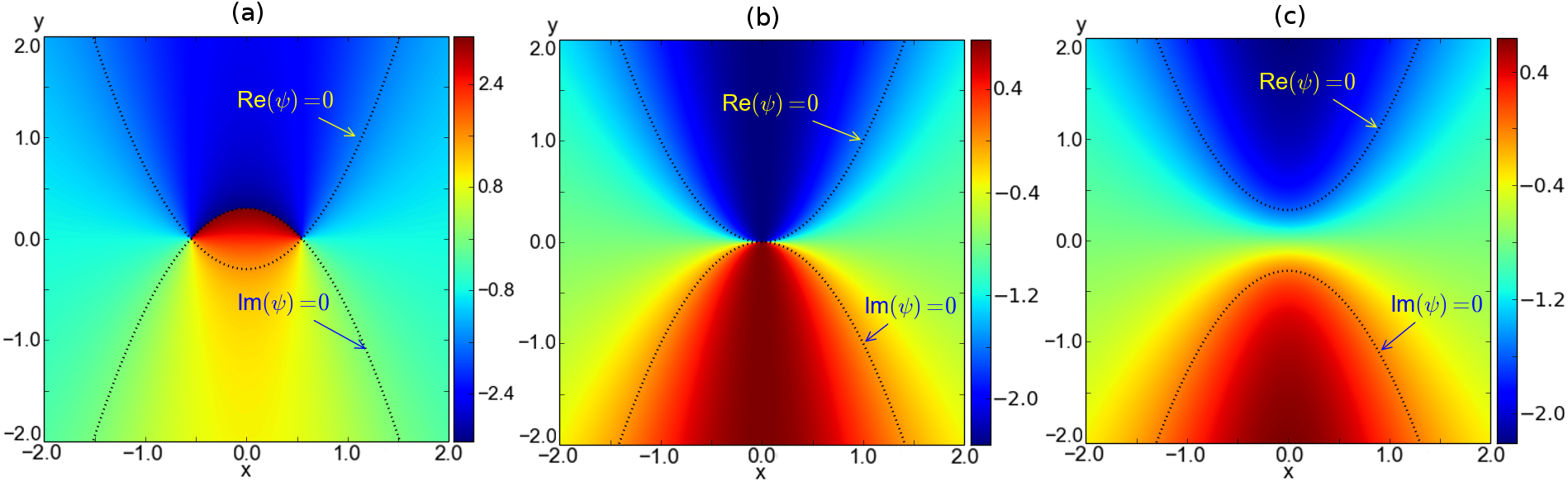
Figure 2: (color online) Annihilation or creation of a vortex pair. The sequence (a)-(b)-(c) corresponds to the annihilation process, while the inverse sequence (c)-(b)-(a) corresponds to the pair-creation process. Such sequences also describe the recombination process of 3D vortex lines, where the depicted plane crosses the recombination point.

Reconnection of Lines and Creation/Annihilation of pairs

An interesting situation occurs when the $R=0$ and $I=0$ lines touch each other tangentially at a single point as in Fig. 2(b). Actually, Fig. 2 can illustrate either the situation right at the beginning of a vortex-pair creation process or at the end of a vortex-pair annihilation process. Indeed, the sequence (a)-(b)-(c) in Fig. 2 exemplifies a vortex-pair annihilation process, while the inverse sequence (c)-(b)-(a) describes a pair-creation process. For simplicity, without loss of generality, one can consider that the lines touch at $x_{0}=y_{0}=t_{0}=0$ and are tangent to the $x$ axis at this point, i.e., $\partial_{x_{0}}R=\partial_{x_{0}}I=0$. At the vicinity of the touching point the Taylor expansion can be used:

$$R = \frac{\partial R}{\partial y_{0}}y+\frac{\partial R}{\partial t_{0}}t+\frac{1}{2}\frac{\partial^{2}R}{\partial x_{0}^{2}}x^{2}+\cdots,$$ (42)

$$I = \frac{\partial I}{\partial y_{0}}y+\frac{\partial I}{\partial t_{0}}t+\frac{1}{2}\frac{\partial^{2}I}{\partial x_{0}^{2}}x^{2}+\cdots.$$ (43)

Close to the touching point, the curves $R=0$ and $I=0$ can then be obtained by considering the dominant terms in (42) and (43), according to

$$y_{{\rm Re}} \approx -\frac{1}{2}\frac{\partial^{2}R/\partial x_{0}^{2}}{\partial R/\partial y_{0}}x^{2}-\frac{\partial R/\partial t_{0}}{\partial R/\partial y_{0}}t,$$ (44)

$$y_{{\rm Im}} \approx -\frac{1}{2}\frac{\partial^{2}I/\partial x_{0}^{2}}{\partial I/\partial y_{0}}x^{2}-\frac{\partial I/\partial t_{0}}{\partial I/\partial y_{0}}t.$$ (45)

The crossing points as depicted in Fig. 2(a) are solutions of the condition $y_{{\rm Re}}=y_{{\rm Im}}$, which are given by

$$x^{2} \approx 2t\alpha,$$ (46)

$$\alpha = \left.\frac{\partial_{t}R\partial_{y}I-\partial_{t}I\partial_{y}R}{\partial_{x}^{2}I\partial_{y}R-\partial_{x}^{2}R\partial_{y}I}\right|_{x=y=t=0}.$$ (47)

The sign of $\alpha$ indicates whether there are real solutions for $x$ with $t<0$ or with $t>0$, thus determining if it is the case of an annihilation ($\alpha<0$) or creation ($\alpha>0$) process. Also from (46), we get the power-law behavior for the creation or annihilation process:

$$x\sim\pm t^{1/2}.$$ (48)

Observe that these results can also be directly obtained from (37) by considering the expansions (42) and (43) and neglecting the subdominant terms. This calculation would then lead to

$$w^{y} \approx -\left.\frac{\partial_{t}R\partial_{x}^{2}I-\partial_{t}I\partial_{x}^{2}R}{\partial_{x}^{2}I\partial_{y}R-\partial_{x}^{2}R\partial_{y}I}\right|_{x=y=t=0},$$ (49)

$$w^{x} \approx \frac{1}{x}\left(\left.\frac{\partial_{t}R\partial_{y}I-\partial_{t}I\partial_{y}R}{\partial_{x}^{2}I\partial_{y}R-\partial_{x}^{2}R\partial_{y}I}\right|_{x=y=t=0}\right)=\frac{\alpha}{x}.$$ (50)

Creation and annihilation of vortex pairs also leave their signatures in the hydrodynamic equation (28). A direct evaluation of $F_{\mu\nu}$ at $t=0$ and around the point $x_{0}=y_{0}=0$ can be obtained with the help of Eqs. (42) and (43). It then gives

$$F_{\mu\nu}=4\pi\delta(x^{2})\delta(y)\frac{\partial_{\mu}R\partial_{\nu}I-\partial_{\nu}R\partial_{\mu}I}{\left|\partial_{x}^{2}R\partial_{y}I-\partial_{x}^{2}I\partial_{y}R\right|}.$$ (51)

Since $\partial_{x}R=\partial_{x}I=0$ at $x=y=0$, the vorticity $\omega=\varepsilon^{ij}F_{ij}$ vanishes. However, it does not mean that the vorticity flux vanishes in all directions. Actually, the vorticity flux in the $y$-direction $\Omega^{2}=F_{01}$ vanishes, while for the $x$-direction we have

$$\Omega^{1}=-F_{02}=-4\pi\delta(x^{2})\delta(y)\frac{\partial_{t}R\partial_{y}I-\partial_{y}R\partial_{t}I}{\left|\partial_{x}^{2}R\partial_{y}I-\partial_{x}^{2}I\partial_{y}R\right|}.$$ (52)

This reflects the fact that although no vortex actually exists at $t=0$, a vorticity flux is still necessary to account for the creation and annihilation of vortex pairs occurring in the superfluid. Also the possibility of having a nonzero $E_{i}=F_{0i}$, even in the absence of vortices, shows that the hydrodynamic equation (28) is capable of describing the creation and annihilation of vortex pairs.

Again, it should be emphasized that such a two-dimensional analysis can also be directly generalized to the case of recombinations of 3D vortex lines by considering planes crossed by the vortex lines. Indeed, the present analysis demonstrates exactly the $x\sim\pm t^{1/2}$ behavior for the reconnection of vortex lines which was observed experimentally in Ref. Paoletti20101367 , numerically in the context of Biot-Savart models in Ref. PhysRevLett.55.1749 , and analytically in the context of GP equation in Ref. Nazarenko2003 . In addition, such a $t^{1/2}$ law turns out to be very general in the sense that it is not restricted to any particular superfluid model such as the GP equation. Indeed, this result depends only on the existence of the first time derivative as well as the first and second spacial derivatives of $\psi$.

Conclusions

This work provides a general framework for the construction of hydrodynamic theories which are capable of correctly including any possible vortex dynamics that may exist in a large set of superfluidity models. By a detailed examination of the role of the multivalued nature of the phase field $S$ in the vortex dynamics, the general hydrodynamic equation (28) was obtained, where all details of a specific model are introduced through the quantity $v_{0}$, defined in Eq. (16). Such multivaluedness of $S$ demands the introduction of the gauge field $A_{\mu}$, where the time-like component $E_{i}=F_{0i}$ of its force field must be introduced in the hydrodynamic equation (28). The only restriction of this approach is that the equation of motion for the macroscopic wave function $\psi$ must be of first order in time, according to Eq. (4). As a test for the practicality of this approach, the dynamics of 2D point vortices and 3D vortex lines have been considered. It turns out that the numerically observed behavior PhysRevA.77.032107 of point vortices moving over a background density gradient is analytically reproduced in Eq. (41). In addition, the $t^{1/2}$ behavior of creation or annihilation of 2D vortex pairs as well as of 3D vortex line reconnections Paoletti20101367 ; PhysRevLett.55.1749 ; Nazarenko2003 is exactly demonstrated for a large class of superfluid models.

Acknowledgments

Acknowledgements to the National Council for the improvement of Higher Education (CAPES). I wish also to thank A. Novikov, M. C. Tsatsos, and Axel Pelster for reading and commenting on this manuscript.

References

- [1] P. Kapitza. Viscosity of liquid helium below the -point. Nature, 141:74, 1938.
- [2] J. F. Allen and A. D. Misener. Flow of liquid helium II. Nature, 141:75, 1938.
- [3] F. London. The phenomenon of liquid helium and the Bose-Einstein degeneracy. Nature, 141:643, 1938.
- [4] C.J. Pethick and H. Smith. Bose-Einstein Condensation in Dilute Gases (Second Edition). Cambridge University Press, 2008.
- [5] L. Pitaevskii and S. Stringari. Bose-Einstein Condensation and Superfluidity (Second Edition). International series of monographs on physics. Oxford University Press, 2016.
- [6] H. Kleinert. Gauge Field Theory of Vortex Lines in and Superfluid Phase Transition. Phys. Lett., 93A:86, 1982.
- [7] H. Kleinert. Towards a Quantum Field Theory of Defects and Stresses–Quantum Vortex Dynamics in a Film of Superfluid Helium. Int. J. Engng. Sci., 23:927, 1985.
- [8] H. Kleinert. Gauge Fields in Condensed Matter. Vol. 1: Superflow and Vortex Lines (Disorder Fields, Phase Transitions). World Scientific, 1989.
- [9] H. Kleinert. Gauge Fields in Condensed Matter. Vol. 2: Stresses and Defects (Differential Geometry, Crystal Melting). World Scientific, 1989.
- [10] H. Kleinert. Multivalued Fields in Condensed Matter, Electromagnetism, and Gravitation. World Scientific, 2008.
- [11] A. A. Kozhevnikov. Gauge vortex dynamics at finite mass of bosonic fields. Phys. Rev. D, 59:085003, Mar 1999.
- [12] A. A. Kozhevnikov. Vortex dynamics in nonrelativistic abelian higgs model. Physics Letters B, 750:122, 2015.
- [13] F. Lund and T. Regge. Unified approach to strings and vortices with soliton solutions. Phys. Rev. D, 14:1524, 1976.
- [14] M. Franz. Vortex-boson duality in four space-time dimensions. Europhys. Lett., 77(4):47005, 2007.
- [15] J. R. Anglin. Vortices near surfaces of Bose-Einstein condensates. Phys. Rev. A, 65:063611, 2002.
- [16] A. Klein, I. L. Aleiner, and Agam O. The internal structure of a vortex in a two-dimensional superfluid with long healing length and its implications. Annals of Physics, 346:195, 2014.
- [17] V.N. Popov. Functional Integrals in Quantum Field Theory and Statistical Physics. Boston, 1983.
- [18] R. P. Feynman. Application of quantum mechanics to liquid helium. Prog. Low Temp. Phys., 1:17, 1955.
- [19] E. A. L. Henn, J. A. Seman, G. Roati, K. M. F. Magalhães, and V. S. Bagnato. Emergence of turbulence in an oscillating Bose-Einstein condensate. Phys. Rev. Lett., 103:045301, 2009.
- [20] L. Skrbek and K. R. Sreenivasan. Developed quantum turbulence and its decay. Phys. Fluids, 24:011301, 2012.
- [21] C. F. Barenghi, V. S. L’vov, and P.-E. Roche. Experimental, numerical, and analytical velocity spectra in turbulent quantum fluid. Proc. Natl. Acad. Sci. U.S.A., 111:4683, 2014.
- [22] M. C. Tsatsos, P. E. S. Tavares, A. Cidrim, A. R. Fritsch, M. A. Caracanhas, F. E. A. dos Santos, C. F. Barenghi, and V. S. Bagnato. Quantum turbulence in trapped atomic bose-einstein condensates. Physics Reports, 622:1, 2016.
- [23] C. F. Barenghi, L. Skrbek, and K. R. Sreenivasan. Introduction to quantum turbulence. Proc. Natl. Acad. Sci. U.S.A., 111:4647, 2014.
- [24] M. T. Reeves, T. P. Billam, B. P. Anderson, and A. S. Bradley. Inverse energy cascade in forced two-dimensional quantum turbulence. Phys. Rev. Lett., 110:104501, 2013.
- [25] M. Kobayashi and M. Tsubota. Kolmogorov spectrum of superfluid turbulence: numerical analysis of the Gross-Pitaevskii equation with a small-scale dissipation. Phys. Rev. Lett., 94:065302, 2005.
- [26] A. Cidrim, F. E. A. dos Santos, L. Galantucci, V. S. Bagnato, and C. F. Barenghi. Controlled polarization of two-dimensional quantum turbulence in atomic bose-einstein condensates. Phys. Rev. A, 93:033651, 2016.
- [27] H. E. Hall and W.F. Vinen. The rotation of liquid Helium II. I. Experiments on the propagation of second sound in uniformly rotating Helium II. Proc. R. Soc. Lond., 238:204, 1956.
- [28] H. E. Hall and W.F. Vinen. The rotation of liquid Helium II. II. The theory of mutual friction in uniformly rotating Helium II. Proc. R. Soc. Lond., 238:215, 1956.
- [29] K. W. Schwarz. Three-dimensional vortex dynamics in superfluid : Line-line and line-boundary interactions. Phys. Rev. B, 31:5782, 1985.
- [30] I. Bialynicki-Birula, Z. Bialynicka-Birula, and C. Śliwa. Motion of vortex lines in quantum mechanics. Phys. Rev. A, 61:032110, 2000.
- [31] P. Mason and N. G. Berloff. Motion of quantum vortices on inhomogeneous backgrounds. Phys. Rev. A, 77:032107, 2008.
- [32] M. S. Paoletti, M. E. Fisher, and D. P. Lathrop. Reconnection dynamics for quantized vortices. Physica D: Nonlinear Phenomena, 239(14):1367, 2010.
- [33] E. D. Siggia and A. Pumir. Incipient singularities in the navier-stokes equations. Phys. Rev. Lett., 55:1749, 1985.
- [34] S. Nazarenko and R. West. Analytical solution for nonlinear schrödinger vortex reconnection. J. Low Temp. Phys., 132(1):1, 2003.