Service Rate Control For Jobs with Decaying Value

Abstract

The task of completing jobs with decaying value arises in a number of application areas including healthcare operations, communications engineering, and perishable inventory control. We consider a system in which a single server completes a finite sequence of jobs in discrete time while a controller dynamically adjusts the service rate. During service, the value of the job decays so that a greater reward is received for having shorter service times. We incorporate a non-decreasing cost for holding jobs and a non-decreasing cost on the service rate. The controller aims to minimize the total cost of servicing the set of jobs. We show that the optimal policy is non-decreasing in the number of jobs remaining – when there are more jobs in the system the controller should use a higher service rate. The optimal policy does not necessarily vary monotonically with the residual job value, but we give algebraic conditions which can be used to determine when it does. These conditions are then simplified in the case that the reward for completion is constant when the job has positive value and zero otherwise. These algebraic conditions are interesting because they can be verified without using algorithms like value iteration and policy iteration to explicitly compute the optimal policy. We also discuss some future modeling extensions.

I Introduction

There are a variety of queueing applications for which job completion rewards decay over time. For example, this is the case in healthcare systems. In some situations, the patients can be treated like “jobs” and the decaying “reward” is the decaying patient health – patients’ health will typically decay as treatment is delayed and this can reduce the efficacy of medical procedures [1]. Jobs can also represent diagnostic tests. A study showed that a majority of primary care physicians were dissatisfied with delays in viewing test results and that these delays can lead to further delays in treatment [2]. The negative impact of patient mortality motivates the general study of queueing for jobs with decaying value.

There are also applications in communications engineering. A notable example is that of multimedia streaming over wireless. Each packet is a job which is completed when the packet is successfully transmitted over a noisy channel. For the sake of maintaining a high quality user experience, multimedia traffic requires low latency as well as low jitter. The real-time nature of streaming means that the packets rapidly decay to having zero value. This has led to a number of interesting practical and theoretical problems in the wireless communications literature. One key problem is that of packet scheduling for downlink cellular systems. In these systems, cellular base-stations need to schedule many different traffic streams while taking into account channel conditions in order to maintain high quality-of-service (QoS) for all users [3]. In other contexts, delay sensitive service becomes relevant for transmitter power control with constraints on inter-departure times [4]. Higher transmitter power gives a higher probability of successful packet transmission so there is a natural trade-off between power usage and delay.

A third application area is that of perishable inventory control. Food items can be modeled as “jobs” while the process of selling to consumers can be modeled as “service”. For example, food items will decay with time as they eventually spoil, at which point they have no value. In these models, the value of food items will decay differently under varying storage and service conditions giving rise to many scheduling and service rate control problems. See [5] for a survey.

Aside from applications oriented research, there is a considerable body of theoretical work geared towards queueing systems for jobs with decaying value. In [6], “impatient” users in an M/M/1 queue are scheduled under the constraint that the rewards for servicing each user decay exponentially. Stochastic depletion problems cover a broad range of preemptive scheduling problems in which items are processed while the rewards for doing so decay over time. In [7], greedy scheduling policies for such problems are shown to be suboptimal by no more than a factor of 2.

In this paper, we consider the following type of system: A finite set of identical jobs are sequentially serviced by a single server in discrete time. The controller chooses the probability that the current head-of-line (HOL) job will reach completion in the current time slot. When a job reaches the server, it has an initial value. This value decays during service and the controller gains a positive reward (i.e. negative cost) when the service is completed. When the value of the job reaches zero, the job is ejected from the system. Non-negative costs are incurred in each time slot for holding the residual jobs as well as for the choice of service probability. We seek to minimize the total cost incurred for servicing the set of jobs.

One of the unique features of this model is that the value decay only occurs during service. This is motivated by several specific applications. In wireless streaming, we have previously considered a similar model in which the value decay follows a step function so that jobs essentially have service time constraint [4][8]. The idea is that when multimedia is streamed over wireless, it is important to maintain a regular stream of information. Because information is encoded across packets, it can be better to drop packets and degrade the quality of the stream rather than delay the entire stream; the service time constraints enforce this behavior. In perishable inventory control, having decay during service but not during storage models the idea that decay happens on different time scales. For example, the quality of certain food items decay very slowly (practically not at all) if stored properly but will decay rapidly during transportation and processing.

Because we focus on this specific type of value decay, this work expands on and partially complements the existing literature. For instance, others have studied monotonicity properties of the optimal service rate control policy for a continuous time Markovian queue with jobs whose value does not decay [9]. In the operations research community, there has also been work on myopic policies for non-preemptive scheduling of jobs whose value decays over the entire sojourn time rather than just during service [10]. Note that a model in which job value decays during the entire sojourn time does not encompass the problem of having job value decay only during service.

The remainder of the paper is organized as follows. In Sec. II, we mathematically define the aforementioned system. This allows us to formulate the problem in a dynamic programming [11] framework. In Sec. III, we numerically demonstrate some of the salient structural features of optimal policies. In particular, we comment on monotonicity of the policies as the number of jobs decreases and as the HOL job value decreases. In Sec. IV, we prove sufficient (and in some cases also necessary) conditions for these observed monotonicity properties to hold. We identify future areas of research in Sec. V and conclude in Sec. VI.

II System Model and Optimal Control

In this section, we mathematically define the system of interest. We describe the dynamics as well as the costs. We formulate the optimal control in a dynamic programming [11] framework and use some results on stochastic shortest path problems [12] to show that optimal policies exist.

A finite set of $B\in\mathbb{Z}_{>0}$ identical jobs is sequentially served in discrete time indexed by $t\in\mathbb{Z}_{\geq 0}$. The number of jobs in the system in time slot $t$ is $b_{t}$. When a job initially reaches the head-of-line (HOL) in time slot $t$, it has a value of $v_{t}=V\in\mathbb{Z}_{>0}$. In time slot $t$, the HOL job completes service with probability $s_{t}\in\mathcal{S}\subseteq[0,1]$ which is chosen by the controller. If the service is not completed, the value is decremented by one. The service attempt in time slot $t$ is independent of all other service attempts. When the HOL job value reaches zero, the job is ejected from the queue and the next job takes the HOL. The system terminates when all jobs have either been serviced or ejected.

Let $\mathcal{B}=\left\{1,2,\ldots,B\right\}$, $\mathcal{V}=\left\{1,2,\ldots,V\right\}$, and $\mathcal{X}=(\mathcal{B}\times\mathcal{V})\cup\left\{(0,V)\right\}$. The state will be taken as the remaining number of jobs in the system and the remaining value of the HOL job so the state at time $t$ is then given by $(b_{t},v_{t})\in\mathcal{X}$. Let $\left\{w_{t}\right\}_{t=0}^{\infty}$ be an IID $\text{Uniform}[0,1]$ noise source. We can write the state update function as follows:

$$(b_{t+1},v_{t+1}) =F(b_{t},v_{t},s_{t},w_{t})$$

$$=\left\{\begin{array}[]{ll}(b_{t},v_{t}-1)&;b_{t}>0,w_{t}>s_{t},v_{t}>1\\ (b_{t}-1,V)&;b_{t}>0,w_{t}>s_{t},v_{t}=1\\ (b_{t}-1,V)&;b_{t}>0,w_{t}\leq s_{t}\\ (0,V)&;b_{t}=0\end{array}\right.$$

We assume that $\mathcal{S}$ is finite. The set of admissible control policies is given by

$$\Pi=\left\{\pi:\mathcal{X}\rightarrow\mathcal{S}\right\}.$$

The cost per time slot of service is $c:\mathcal{S}\rightarrow\mathbb{R}_{\geq 0}$. The cost per time slot of holding jobs is $h:\mathcal{B}\rightarrow\mathbb{R}_{\geq 0}$. The reward for servicing a job is given by $r:\mathcal{V}\rightarrow\mathbb{R}_{>0}$. Therefore, if the HOL job completes service when it has residual value $v$, the cost is given by $-r(v)$. Although $r(\cdot)$ is positive and only defined on $\mathcal{V}$, the dynamics logically suggest that $r(0)=0$ since jobs with zero value are ejected. We assume that $c(\cdot)$, $h(\cdot)$, and $r(\cdot)$ are each non-decreasing. If we let $\mathbb{I}_{\left\{\cdot\right\}}$ be the indicator function, we can define the stage cost in time slot $t$ as

$$G(b_{t},v_{t},s_{t},w_{t}) =\mathbb{I}_{\left\{b_{t}>0\right\}}\left(h(b_{t})+c(s_{t})-\mathbb{I}_{\left\{w_{t}\leq s_{t}\right\}}r(v_{t})\right).$$

Given the initial state is $(b,v)\in\mathcal{X}$, we define the optimal cost-to-go as follows:

$$\mathcal{J} (b,v)$$

$$=\min_{\pi\in\Pi}\mathbb{E}\left[\left.\sum_{t=0}^{\infty}G(b_{t},v_{t},\pi(b_{t},v_{t}),w_{t})\right|(b_{0},v_{0})=(b,v)\right]$$

The system reaches the terminal state $(0,V)$ with probability one in at most $BV$ time slots. In addition, $\mathcal{B}$ and $\mathcal{V}$ are finite so the costs are bounded (though not necessarily non-negative). Therefore, $\mathcal{J}(b,v)$ is well defined for all $(b,v)\in\mathcal{X}$.

Because the control policies select probability distributions on the state transitions, we have a stochastic shortest path problem. By assumption, $\mathcal{S}$ is finite so this can be solved using standard techniques like value iteration and policy iteration [12]. Hence, we have the following Bellman equation

$$\mathcal{J} (b,v)=\min_{s\in\mathcal{S}}\Big{\{}c(s)+h(b)$$

$$+s[-r(v)+\mathcal{J}(b-1,V)]$$

$$+(1-s)[\mathcal{J}(b,v-1)\mathbb{I}_{\left\{v>1\right\}}+\mathcal{J}(b-1,V)\mathbb{I}_{\left\{v=1\right\}}]\Big{\}}$$

with the boundary condition that $\mathcal{J}(0,V)=0$. In general, there can be multiple optimal policies but we will refer to the optimal policy as

$$\mu (b,v)=\min\operatorname*{argmin}_{s\in\mathcal{S}}\Big{\{}c(s)+h(b)$$

$$+s[-r(v)+\mathcal{J}(b-1,V)]$$

$$+(1-s)[\mathcal{J}(b,v-1)\mathbb{I}_{\left\{v>1\right\}}+\mathcal{J}(b-1,V)\mathbb{I}_{\left\{v=1\right\}}]\Big{\}}$$

with $\mu(0,V)$ being arbitrary because $(0,V)$ is a cost-free trapping state. Again, since we are solving a stochastic shortest path problem, $\mu$ can be computed by using either value iteration or policy iteration [12].

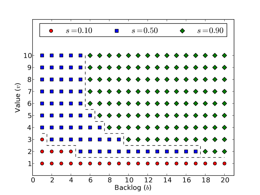
(a)

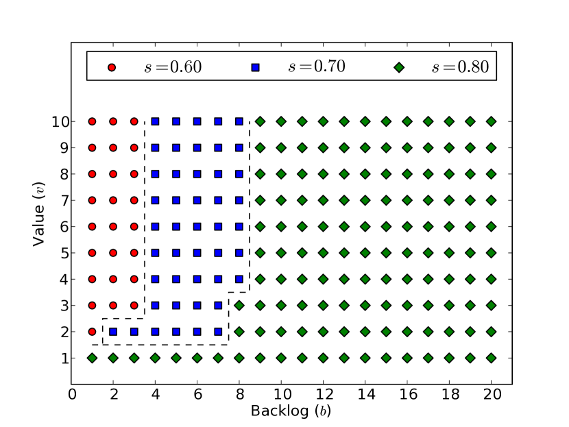
(b)

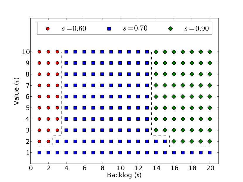
(c)

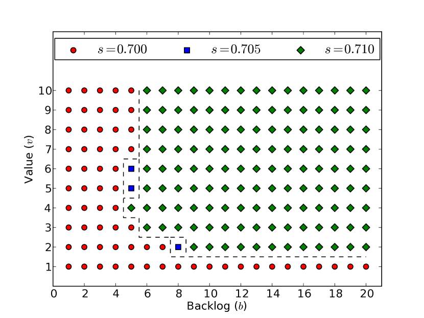
(d)

Figure 1: Examples of $\mu$ for different system parameters. For each $(b,v)\in\mathcal{B}\times\mathcal{V}$, we plot a point to indicate the value of $\mu(b,d)$. The dashed lines segment the state space to show when the policy changes. For each of the following policies, we take $h(b)=b$, $c(s)=5\ln\left(\frac{1}{1-s}\right)$, $V=10$, and $B=20$. For Fig. 1a, $r(v)=v$ and $\mathcal{S}=\left\{0.1,0.5,0.9\right\}$. In this case, $b\mapsto\mu(b,v)$ is non-decreasing for all $v\in\mathcal{V}$ and $v\mapsto\mu(b,v)$ is non-decreasing for all $b\in\mathcal{B}$. For Fig. 1b, $r(v)=\frac{v}{10}+25$ and $\mathcal{S}=\left\{0.6,0.7,0.8\right\}$. In this case, $b\mapsto\mu(b,v)$ is non-decreasing for all $v\in\mathcal{V}$ and $v\mapsto\mu(b,v)$ is non-increasing for all $b\in\mathcal{B}$. For Fig. 1c, $r(v)=\frac{v}{10}+20$ and $\mathcal{S}=\left\{0.6,0.7,0.9\right\}$. In this case, $b\mapsto\mu(b,v)$ is non-decreasing for all $v\in\mathcal{V}$ while the monotonicity of $v\mapsto\mu(b,v)$ varies with $b$. For Fig. 1d, $r(v)=5\ln(1+v)$ and $\mathcal{S}=\left\{0.700,0.705,0.710\right\}$. In this case, $b\mapsto\mu(b,v)$ is non-decreasing for all $v\in\mathcal{V}$ while $v\mapsto\mu(b,v)$ is not necessarily monotone in anyway; note that $v\mapsto\mu(5,v)$ is neither non-decreasing nor non-increasing.

III Numerical Experiments

In this section we offer a brief numerical investigation of the optimal policy under different conditions. This allows us to demonstrate the potential structural properties of $\mu$. In each case we observe that $b\mapsto\mu(b,v)$ is non-decreasing. We observe that similar monotonicity properties do not always hold for $v\mapsto\mu(b,v)$. This motivates the analytic investigation in Sec. IV.

For each of the following policies, we take $h(b)=b$, $c(s)=5\ln\left(\frac{1}{1-s}\right)$, $V=10$, and $B=20$. We vary $r(\cdot)$ and $\mathcal{S}$ to demonstrate different structural features. Note that even though $c(1)=\infty$, in each example $1\not\in\mathcal{S}$ so the boundedness of $c(\cdot)$ is not violated. These parameters are not intended to model a specific system and have been chosen for illustrative purposes.

For Fig. 1a, $r(v)=v$ and $\mathcal{S}=\left\{0.1,0.5,0.9\right\}$. In this case, $b\mapsto\mu(b,v)$ is non-decreasing for all $v\in\mathcal{V}$ and $v\mapsto\mu(b,v)$ is non-decreasing for all $b\in\mathcal{B}$. To anthropomorphize these properties, we can think of the server “giving up” on a particular job as the job value decreases. Similarly, the server generally “tries harder” when there are more jobs remaining to be served.

For Fig. 1b, $r(v)=\frac{v}{10}+25$ and $\mathcal{S}=\left\{0.6,0.7,0.8\right\}$. In this case, $b\mapsto\mu(b,v)$ is non-decreasing for all $v\in\mathcal{V}$ and $v\mapsto\mu(b,v)$ is non-increasing for all $b\in\mathcal{B}$. The server still “tries harder” when there are more jobs remaining, but the server also “tries harder” as the value of the HOL job decays. This shows that in some cases, it is optimal for the server to try to complete jobs even when they have low residual value.

For Fig. 1c, $r(v)=\frac{v}{10}+20$ and $\mathcal{S}=\left\{0.6,0.7,0.9\right\}$. In this case, $b\mapsto\mu(b,v)$ is non-decreasing for all $v\in\mathcal{V}$ while the monotonicity of $v\mapsto\mu(b,v)$ varies with $b$. As in the previous two cases, the server “tries harder” when there are more jobs remaining. However, the monotonicity of $v\mapsto\mu(b,v)$ depends on $b$. This demonstrates that although it can be optimal for the server to complete jobs with low residual value, this behavior depends on how many other jobs are waiting to be served.

For Fig. 1d, $r(v)=5\ln(1+v)$ and $\mathcal{S}=\left\{0.700,0.705,0.710\right\}$. In this case, $b\mapsto\mu(b,v)$ is non-decreasing for all $v\in\mathcal{V}$ while $v\mapsto\mu(b,v)$ is not necessarily monotone in anyway; note that $v\mapsto\mu(5,v)$ is neither non-decreasing nor non-increasing. In this final case, we again see that the server “tries harder” when there are more jobs remaining. However, $v\mapsto\mu(b,v)$ does not exhibit either the “try harder” or the “give up” behaviors.

IV Monotonicity of the Optimal Policy

The numerical examples from the previous section demonstrate the potentially rich structure of $\mu$. The monotonicity properties that often hold are interesting because they offer structural insights and intuitive explanations. However, it is not immediately clear what conditions are necessary in order to guarantee that these properties hold. In this section we show that because $h(\cdot)$ is non-decreasing, $b\mapsto\mu(b,v)$ will be non-decreasing for each $v\in\mathcal{V}$. We also provide algebraic conditions for determining the monotonicity of $v\mapsto\mu(b,v)$. These algebraic conditions are valuable because they can be verified without explicitly solving for $\mu$. In the case that $r(\cdot)$ is constant, we provide a simpler algebraic condition which is similar to the one provided in [4].

We start with some useful definitions.

Definition 1

For each $b\in\mathcal{B}$, let $\delta(b,0)=0$ and $\sigma(b,0)=0$. For each $(b,v)\in\mathcal{B}\times\mathcal{V}$, define $\delta(b,v)$ and $\sigma(b,v)$ as follows:

$$\delta(b,v) =h(b)+\min_{s\in\mathcal{S}}\left\{c(s)-s\left[r(v)+\sum_{i=0}^{v-1}\delta(b,i)\right]\right\}$$

$$\sigma(b,v) =\sum_{i=0}^{v}\delta(b,i)$$

For each $(b,v)\in\mathcal{B}\times\mathcal{V}$ define $T_{b,v}:\mathbb{R}\rightarrow\mathbb{R}$ as follows:

$$T_{b,v}(x)=x+h(b)+\min_{s\in\mathcal{S}}\{c(s)-s[r(v)+x]\}$$

Proposition 1

For each $(b,v)\in\mathcal{B}\times\mathcal{V}$, the Bellman equation can be characterized as follows:

$$\mathcal{J}(b,v)=\left\{\begin{array}[]{ll}\mathcal{J}(b-1,V)+\delta(b,1)&,v=1\\ \mathcal{J}(b,v-1)+\delta(b,v)&,v>1\end{array}\right.$$

Furthermore, the optimal policy can be written as

$$\mu(b,v)=\min\operatorname*{argmin}_{s\in\mathcal{S}}\left\{c(s)-s\left[r(v)+\sigma(b,v-1)\right]\right\}.$$

Proof:

For any fixed $b\in\mathcal{B}$, we apply the principle of strong mathematical induction on $v\in\mathcal{V}$. For $v=1$, we merely need to re-order the Bellman equation:

$$\mathcal{J} (b,1)$$

$$=\min_{s\in\mathcal{S}}\Big{\{}c(s)+h(b)$$

$$+s[-r(1)+\mathcal{J}(b-1,V)]+(1-s)\mathcal{J}(b-1,V)\Big{\}}$$

$$=\mathcal{J}(b-1,V)+h(b)$$

$$+\min_{s\in\mathcal{S}}\Big{\{}c(s)+s[-r(1)+\mathcal{J}(b-1,V)]-s\mathcal{J}(b-1,V)\Big{\}}$$

$$=\mathcal{J}(b-1,V)+h(b)+\min_{s\in\mathcal{S}}\left\{c(s)-sr(1)\right\}$$

$$=\mathcal{J}(b-1,V)+\delta(b,1)$$

We now use this for $v=2$:

$$\mathcal{J}(b,2) =\min_{s\in\mathcal{S}}\Big{\{}c(s)+h(b)$$

$$+s[-r(2)+\mathcal{J}(b-1,V)]+(1-s)\mathcal{J}(b,1)\Big{\}}$$

$$=\mathcal{J}(b,1)+h(b)$$

$$+\min_{s\in\mathcal{S}}\left\{c(s)+s[-r(2)+\mathcal{J}(b-1,V)-\mathcal{J}(b,1)]\right\}$$

$$=\mathcal{J}(b,1)+h(b)+\min_{s\in\mathcal{S}}\left\{c(s)-s[r(2)+\delta(b,1)]\right\}$$

$$=\mathcal{J}(b,1)+\delta(b,2)$$

Now assume that the proposition holds for $\left\{1,\ldots,v\right\}\subsetneq\mathcal{V}$.

$$\mathcal{J}(b,v+1)$$

$$=\min_{s\in\mathcal{S}}\Big{\{}c(s)+h(b)$$

$$+s[-r(v+1)+\mathcal{J}(b-1,V)]+(1-s)\mathcal{J}(b,v)\Big{\}}$$

$$=\mathcal{J}(b,v)+h(b)$$

$$+\min_{s\in\mathcal{S}}\left\{c(s)+s[-r(v+1)+\mathcal{J}(b-1,V)-\mathcal{J}(b,v)]\right\}$$

$$=\mathcal{J}(b,v)+h(b)+\min_{s\in\mathcal{S}}\Big{\{}c(s)-s[r(v+1)$$

$$+\sum_{i=2}^{v}(\mathcal{J}(b,i)-\mathcal{J}(b,i-1))+(\mathcal{J}(b,1)-\mathcal{J}(b-1,V))]\Big{\}}$$

Now we apply the induction hypothesis to write sum in the final line in terms of $\delta(b,i)$. We then use the definitions of $\delta(b,v+1)$ and $\sigma(b,v)$ to complete the proof.

$$\mathcal{J}(b,v+1)$$

$$=\mathcal{J}(b,v)+h(b)+\min_{s\in\mathcal{S}}\left\{c(s)-s[r(v+1)+\sum_{i=0}^{v}\delta(b,i)]\right\}$$

$$=\mathcal{J}(b,v)+h(b)+\min_{s\in\mathcal{S}}\left\{c(s)-s[r(v+1)+\sigma(b,v)]\right\}$$

$$=\mathcal{J}(b,v)+\delta(b,v+1)$$

Now that we have this alternative characterization of the Bellman equation, we simply ignore the terms which do not involve $s$ to conclude that

$$\mu(b,v)=\min\operatorname*{argmin}_{s\in\mathcal{S}}\left\{c(s)-s\left[r(v)+\sigma(b,v-1)\right]\right\}.$$

∎

This reformulation will be useful for determining the monotonicity properties of $\mu$. To do so, we will make use of the following definition and theorem (a version of Topkis’s Theorem [13]).

Lemma 1

Let $\mathcal{D}_{1}\subseteq\mathbb{R}$ and $\mathcal{D}_{2}\subseteq\mathbb{R}$ be non-empty and suppose $f:\mathcal{D}_{1}\times\mathcal{D}_{2}\rightarrow\mathbb{R}$ satisfies the following inequality for all $d_{1}^{-}\leq d_{1}^{+}$ and $d_{2}^{-}\leq d_{2}^{+}$:

$$f(d_{1}^{+},d_{2}^{+}) +f(d_{1}^{-},d_{2}^{-})\leq f(d_{1}^{+},d_{2}^{-})+f(d_{1}^{-},d_{2}^{+})$$

Then $f$ is submodular. If $f$ is submodular and we define $g:\mathcal{D}_{2}\rightarrow\mathcal{D}_{1}$ as

$$g(d_{2})=\min\operatorname*{argmin}_{d_{1}\in\mathcal{D}_{1}}f(d_{1},d_{2})$$

then $g(\cdot)$ is non-decreasing.

Proposition 2

There exists a non-decreasing function $g:\mathbb{R}\rightarrow\mathcal{S}$ such that $\mu(b,v)=g(r(v)+\sigma(b,v-1))$.

Proof:

Let $f:\mathcal{S}\times\mathbb{R}\rightarrow\mathbb{R}$ be defined by $f(s,x)=c(s)-sx$. Take $s^{+}\geq s^{-}$ and $x^{+}\geq x^{-}$. $f$ is submodular if

$$f(s^{+},x^{+})+f(s^{-},x^{-})\leq f(s^{+},x^{-})+f(s^{-},x^{+}).$$

Let $LHS$ and $RHS$ denote the left and right sides of the previous inequality.

$$LHS-RHS =(c(s^{+})-s^{+}x^{+}+c(s^{-})-s^{-}x^{-})$$

$$-(c(s^{+})-s^{+}x^{-}+c(s^{-})-s^{-}x^{+})$$

$$=s^{+}x^{-}+s^{-}x^{+}-s^{+}x^{+}-s^{-}x^{-}$$

$$=(s^{+}-s^{-})(x^{-}-x^{+})$$

$(s^{+}-s^{-})\geq 0$ and $(x^{-}-x^{+})\leq 0$ so $LHS\leq RHS$ and $f$ is submodular. Let $g$ be defined as

$$g(x)=\min\operatorname*{argmin}_{s\in\mathcal{S}}f(s,x)$$

By Lemma 1, $g(\cdot)$ is non-decreasing and by Proposition 1, $\mu(b,v)=g(r(v)+\sigma(b,v-1))$. ∎

The previous proposition shows that we can determine the monotonicity properties of $\mu$ by understanding the monotonicity properties of $r(v)+\sigma(b,v-1)$. Since $r(v)$ does not depend on $b$, we can study $b\mapsto\sigma(b,v)$ in order to understand $b\mapsto\mu(b,v)$.

Proposition 3

For each $(b,v)\in\mathcal{B}\times\mathcal{V}$, $T_{b,v}(\cdot)$ is non-decreasing and $\sigma(b,v)=T_{b,v}(\sigma(b,v-1))$.

Proof:

Take $x^{+}\geq x^{-}$. For any $s\in\mathcal{S}$, $(1-s)\geq 0$ so $(1-s)x^{+}\geq(1-s)x^{-}$. Adding the same quantity to each side preserves the inequality so

$$h(b)+c(s)-r(v) +(1-s)x^{+}\geq$$

$$h(b)+c(s)-r(v)+(1-s)x^{-}$$

Minimizing over $s\in\mathcal{S}$ and applying the monotonicity of minimization gives us that $T_{b,v}(x^{+})\geq T_{b,v}(x^{-})$.

The second part of the proposition follows from the following algebraic manipulation:

$$\sigma (b,v)$$

$$=\sum_{i=0}^{v}\delta(b,i)=\delta(b,v)+\sigma(b,v-1)$$

$$=h(b)$$

$$+\min_{s\in\mathcal{S}}\left\{c(s)-s\left[r(v)+\sum_{i=0}^{v-1}\delta(b,i)\right]\right\}+\sigma(b,v-1)$$

$$=h(b)$$

$$+\min_{s\in\mathcal{S}}\left\{c(s)-s\left[r(v)+\sigma(b,v-1)\right]\right\}+\sigma(b,v-1)$$

$$=T_{b,v}(\sigma(b,v-1))$$

∎

Theorem 1

For each $v\in\mathcal{V}$, $b\mapsto\mu(b,v)$ is non-decreasing.

Proof:

We prove that $b\mapsto\sigma(b,v)$ is non-decreasing via induction. Because $\mu(b,v)=g(r(v)+\sigma(b,v))$ for some non-decreasing $g$, the result regarding $b\mapsto\mu(b,v)$ follows immediately.

For $v=1$,

$$\sigma(b,v)=\delta(b,1)=h(b)+\min_{s\in\mathcal{S}}\left\{c(s)-sr(1)\right\}.$$

By assumption, $h(\cdot)$ is non-decreasing so $b\mapsto\sigma(b,1)$ is non-decreasing. Now assume that $b\mapsto\sigma(b,v)$ is non-decreasing for some $v\in\mathcal{V}\setminus\left\{V\right\}$. Because $h(\cdot)$ is non-decreasing, $T_{b^{\prime},v}(x)\geq T_{b,v}(x)$ whenever $b^{\prime}\geq b$. In addition, $T_{b,v+1}(\cdot)$ is order-preserving (i.e. non-decreasing) and $\sigma(b,v+1)=T_{b,v+1}(\sigma(b,v))$. Therefore, $b\mapsto\sigma(b,v+1)$ is also non-decreasing. By induction, $b\mapsto\sigma(b,v)$ is non-decreasing for all $v\in\mathcal{V}$. ∎

As demonstrated in Sec. III, the behavior of $v\mapsto\mu(b,v)$ is slightly more nuanced. The following theorem gives a set of algebraic conditions for determining the monotonicity properties of $v\mapsto\mu(b,v)$. These conditions are useful and interesting because they can be verified without computing $\mu$. Furthermore, the proposition relates the rate of decay to the $\delta$ terms. This matches our intuition that the rate of decay should play a role in how the controller adapts to the decay itself.

Theorem 2

Fix any $b\in\mathcal{B}$. If $\delta(b,v)\geq-[r(v+1)-r(v)]$ for all $v\in\mathcal{V}\setminus\left\{V\right\}$, then $v\mapsto\mu(b,v)$ is non-decreasing. If $\delta(b,v)\leq-[r(v+1)-r(v)]$ for all $v\in\mathcal{V}\setminus\left\{V\right\}$, then $v\mapsto\mu(b,v)$ is non-increasing.

Proof:

Fix any $v\in\mathcal{V}\setminus\left\{V\right\}$. By Proposition 2, $\mu(b,v)=g(r(v)+\sigma(b,v-1))$ for some non-decreasing $g(\cdot)$. Therefore, $\mu(b,v+1)\geq\mu(b,v)$ if and only if $r(v+1)+\sigma(b,v)\geq r(v)+\sigma(b,v-1)$.

$$[r(v+1) +\sigma(b,v)]-[r(v)+\sigma(b,v-1)]$$

$$=r(v+1)-r(v)+[\sigma(b,v)-\sigma(b,v-1)]$$

$$=r(v+1)-r(v)+\delta(b,v)$$

So if $\delta(b,v)\geq-[r(v+1)-r(v)]$, then $\mu(b,v+1)\geq\mu(b,v)$. If this holds for every $v\in\mathcal{V}\setminus\left\{V\right\}$, then $v\mapsto\mu(b,v)$ is non-decreasing.

The case for when $\delta(b,v)\leq-[r(v+1)-r(v)]$ is analogous. ∎

When $r(v)$ is constant, we have an even simpler condition for testing the monotonicity of $v\mapsto\mu(b,v)$. Taking $r(v)$ as a constant can be used to model service time constraints; this was the case in the wireless streaming model presented in [4]. In this case, $v\mapsto\mu(b,v)$ is always either non-decreasing or non-increasing. A single algebraic condition can be verified to determine which is the case.

Theorem 3

Suppose $r(v)=\overline{r}>0$ for all $v\in\mathcal{V}$. If

$$h(b)+\min_{s\in\mathcal{S}}\{c(s)-s\overline{r}\}\geq 0$$

then $v\mapsto\mu(b,v)$ is non-decreasing. If

$$h(b)+\min_{s\in\mathcal{S}}\{c(s)-s\overline{r}\}\leq 0$$

then $v\mapsto\mu(b,v)$ is non-increasing.

Proof:

Define $T_{b,\overline{r}}:\mathbb{R}\rightarrow\mathbb{R}$ as follows:

$$T_{b,\overline{r}}(x)=x+h(b)+\min_{s\in\mathcal{S}}\{c(s)-s[\overline{r}+x]\}$$

Note that because $r(v)=\overline{r}$, $T_{b,\overline{r}}(x)=T_{b,v}(x)$ for all $x\in\mathbb{R}$. We are interested in the sign of $T_{b,\overline{r}}(0)$.

Assume that $T_{b,\overline{r}}(0)\geq 0$. We show that $v\mapsto\sigma(b,v)$ is non-decreasing by applying the principle of mathematical induction. Since $\mu(b,v)=g(\overline{r}+\sigma(b,v-1))$ for some non-decreasing $g(\cdot)$, the result follows. The case of $T_{b,\overline{r}}(0)\leq 0$ is analogous.

By Proposition 3, $\sigma(b,1)=T_{b,\overline{r}}(0)$ and $\sigma(b,v+1)=T_{b,\overline{r}}(\sigma(b,v))$ for all $v\in\mathcal{V}\setminus\left\{V\right\}$. Applying $T_{b,\overline{r}}$ to $\sigma(b,1)=T_{b,\overline{r}}(0)\geq 0$ and using the monotonicity of $T_{b,\overline{r}}(\cdot)$ gives us that

$$\sigma(b,2)=T_{b,\overline{r}}(\sigma(b,1))\geq T_{b,\overline{r}}(0)=\sigma(b,1).$$

Now assume that $\sigma(b,v)\geq\sigma(b,v-1)$ for some $v\in\mathcal{V}\setminus\left\{1\right\}$. Then applying $T_{b,\overline{r}}$ to $\sigma(b,v)=T_{b,\overline{r}}(\sigma(b,v-1))$ and using the monotonicity of $T_{b,\overline{r}}(\cdot)$ gives us that

$$\sigma(b,v+1)=T_{b,\overline{r}}(\sigma(b,v))\geq T_{b,\overline{r}}(\sigma(b,v-1))=\sigma(b,v).$$

So by induction, if $T_{b,\overline{r}}(0)\geq 0$ then $\sigma(b,v+1)\geq\sigma(b,v)$ for all $v\in\mathcal{V}\setminus\left\{V\right\}$ and hence, $v\mapsto\sigma(b,v)$ is non-decreasing. ∎

V Future Work

The results in this paper suggest a number of future modeling extensions. For instance, we could consider jobs which have different reward functions. This would make $r(v)$ into $r(v,b)$. In addition, jobs could have different initial values so that instead of $V$ we have $V(b)$. This could potentially lead to notational complications because for $b<b^{\prime}$ we might have that $\mu(b,v)$ is defined but $\mu(b^{\prime},v)$ is not. Having the initial value vary with the job would create “holes” in the state space which could make it cumbersome to discuss how the optimal policy varies with the number of remaining jobs. On the other hand, allowing for these modeling extensions would give more general results.

A more significant modeling extension would be including job arrivals. The proofs in this paper take advantage of the fact that the number of jobs in the system decreases over time. While it is reasonable to conjecture that there are similar monotonicity properties when job arrivals are included, the proofs in this paper would need substantial modification to account for these properties.

VI Conclusion

In this paper we have modeled a system in which jobs are completed by a single server while a controller dynamically adjusts the service rate. The reward for each job completion decays during service. Costs are incurred for holding jobs and for exerting service effort. This can be used as an abstract model for applications in healthcare, information technology, as well as perishable inventory control.

We show that when the holding cost is non-decreasing, the optimal policy will be non-decreasing in the number of remaining jobs. We also give algebraic conditions for determining and verifying the monotonicity of the optimal policy as a function of the residual value. When the reward for job completion is given by a step function, these algebraic conditions collapse into a single inequality that can be used to determine the monotonicity of the optimal policy.

References

- [1] P. McQuillan, S. Pilkington, A. Allan, B. Taylor, A. Short, G. Morgan, M. Nielsen, D. Barrett, and G. Smith, “Confidential inquiry into quality of care before admission to intensive care,” British Medical Journal, vol. 316, no. 7148, pp. 1853–1858, 1998.
- [2] E. G. Poon, T. K. Gandhi, T. D. Sequist, H. J. Murff, A. S. Karson, and D. W. Bates, “’I wish I had seen this test result earlier!’: dissatisfaction with test result management systems in primary care,” Archives of internal medicine, vol. 164, no. 20, pp. 2223–2228, 2004.
- [3] A. Dua, C. W. Chan, N. Bambos, and J. Apostolopoulos, “Channel, deadline, and distortion (CD2) aware scheduling for video streams over wireless,” Wireless Communications, IEEE Transactions on, vol. 9, no. 3, pp. 1001–1011, 2010.
- [4] N. Master and N. Bambos, “Power control for wireless streaming with HOL packet deadlines,” in Communications (ICC), 2014 IEEE International Conference on, pp. 2263–2269, IEEE, 2014.
- [5] S. Nahmias, “Perishable inventory theory: A review,” Operations Research, vol. 30, no. 4, pp. 680–708, 1982.
- [6] A. C. Dalal and S. Jordan, “Optimal scheduling in a queue with differentiated impatient users,” Performance Evaluation, vol. 59, no. 1, pp. 73–84, 2005.
- [7] C. W. Chan and V. F. Farias, “Stochastic depletion problems: Effective myopic policies for a class of dynamic optimization problems,” Mathematics of Operations Research, vol. 34, no. 2, pp. 333–350, 2009.
- [8] N. Master and N. Bambos, “Power control for packet streaming with head-of-line deadlines,” Performance Evaluation (Under review), 2014.
- [9] J. M. George and J. M. Harrison, “Dynamic control of a queue with adjustable service rate,” Operations Research, vol. 49, no. 5, pp. 720–731, 2001.
- [10] N. Master, C. W. Chan, and N. Bambos, “Myopic policies for non-preemptive scheduling of jobs with decaying value,” arXiv preprint arXiv:1606.04136, 2016.
- [11] D. P. Bertsekas, Dynamic programming and optimal control, vol. 1-2. Athena Scientific Belmont, MA, 2005.
- [12] D. P. Bertsekas and J. N. Tsitsiklis, “An analysis of stochastic shortest path problems,” Mathematics of Operations Research, vol. 16, no. 3, pp. 580–595, 1991.
- [13] D. M. Topkis, “Minimizing a submodular function on a lattice,” Operations research, vol. 26, no. 2, pp. 305–321, 1978.