Evolution of the cycles of magnetic activity of the Sun

and Sun-like stars in time

E.A. Bruevich ^a , V.V. Bruevich ^b, B.P. Artamonov ^c

^a,b,c Sternberg Astronomical Institute, Moscow State University,

Universitetsky pr., 13, Moscow 119992, Russia

e-mail: ^ared-field@yandex.ru, ^bbrouev@sai.msu.ru, ^cartamon@sai.msu.ru

Abstract

We applied the method of continuous wavelet-transform to the time-frequency analysis to the sets of observations of relative sunspot numbers, sunspot areas and to 6 Mount Wilson HK-project stars with well-defined magnetic cycles. Wavelet analysis of these data reveals the following pattern: at the same time there are several activity cycles whose periods vary widely from the quasi-biennial up to the centennial period for the Sun and vary significant during observations time of the HK-project stars. These relatively low-frequency periodic variations of the solar and stellar activity gradually change the values of periods of different cycles in time. This phenomenon can be observed in every cycles of activity.

Key words. Solar cycle-observations-solar activity indices.

1 Introduction

The study of magnetic activity of the Sun and the stars which is called by the complex of electromagnetic and hydrodynamic processes in their atmospheres is of fundamental importance for astrophysics.

The relative sunspot number SSN is a very popular, widely used solar activity index: the series of relative sunspot numbers direct observations continue almost two hundred years. The SSN index has an advantage over other indices of activity because data on annual variation available from the 1700’s: for 1700–1849 on the basis of undirect data, later then 1850 – according to the direct observations. The SSN (also known as the International sunspot number, relative sunspot number, or Wolf number) is a quantity that measures the number of sunspots and groups of sunspots present on the surface of the sun. Sunspots are temporary phenomena on the photosphere of the Sun that appear visibly as dark spots compared to surrounding regions. They are caused by intense magnetic activity, which inhibits convection by an effect comparable to the eddy current brake, forming areas of reduced surface temperature. Although they are at temperatures of roughly 3000-4500K), the contrast with the surrounding material at about 5.780 K leaves them clearly visible as dark spots. Manifesting intense magnetic activity, sunspots host secondary phenomena such as coronal loops(prominences) and reconnection events. Most of solar flares and coronal mass ejections originate in magnetically active regions around visible sunspot groupings. Similar phenomena indirectly observed on stars are commonly called stars pots and both light and dark spots have been measured. Thus the cyclic variations of the SSN and the evolution of these cycles in time is an important task for the study of all complex phenomena on the Sun associated with different indices of solar activity.

The historical sunspot record was first put by Wolf in 1850s and has been continued later in the 20th century until today. Wolf’s original definition of the relative sunspot number for a given day as $R=10\cdot$ Number of Groups + Number of Spots visible on the solar disk has stood the test of time. The factor of 10 has also turned out to be a good choice as historically a group contained on average ten spots. Almost all solar indices and solar wind quantities show a close relationship with the SSN, see [1],[2].

We have to point out that close interconnection between radiation fluxes characterized the energy release from different atmosphere’s layers is the widespread phenomenon among the stars of late-type spectral classes, see [3]. It was confirmed that there exists the close interconnection between photospheric and coronal fluxes variations for Sun-like stars of F, G, K and M spectral classes with widely varying activity of their atmospheres, see [4],[5]. It was also shown that the summary areas of spots and values of X-ray fluxes increase gradually from the sun and Sun-like Mount Wilson HK project stars [6] with the low spotted discs to the highly spotted K and M-stars. The main characteristic describing the photospheric radiation is the spottiness of the stars. Thus, the study of the relative sunspot numbers is very important to explain the observations of sun-like stars.

The level of chromospheric activity of the Sun is consistent with that of HK-project stars, which have well-defined cycles of activity, but the level of coronal activity of the Sun is significantly below that of the coronal activity of Sun-like G-stars from the different observational Programs which are studied Sun-like stars: (1) HK-project – the Mount Wilson program, see [6]; (2) The California & Carnegie Planet Search Program which includes observations of approximately 1000 stars at Keck & Lick observatories in chromospheric CaII H&K emission cores, see [7]; (3) The Magellan Planet Search Program which includes Las Campanas Observatory CA measurements of 670 F, G, K and M main sequence stars of the Southern Hemisphere. $S_{HK}$-indexes of these stars are also converted to the Mount Wilson system, see [8].

A comparative analysis of chromospheric, coronal and cyclic activity of the Sun and Sun-like stars of F, G and K spectral classes from these different observational Programs shows the similar characteristics of magnetic cycles on the Sun and on the Sun-like stars, see [9],[10].

We have studied: (1) – yearly averaged values of SSN during solar activity cycles 1 – 23, the tree-hundred yrs data set; (2) – yearly averaged values of sunspot areas A, the 400 yrs data set, see [11]; (3) – monthly averaged values of SSN during activity cycles 18 – 24 and (4)– daily averaged values of SSN during activity cycle 22. All SSN data are available at NGDC web site, see observational data from National Geophysical Data Center. Solar Data Service [12].

For the HK-project stars study we have applied the wavelet analysis for partially available data from the records of relative CaII emission fluxes - the variation of $S_{HK}$-indexes for 1965–1992 observation sets from Baliunas et al. (1995) and for 1985– 2002 observations from [13]. We used the detailed plots of $S_{HK}$-indexes time dependencies: each point of the record of observations, which we processed in this paper using wavelet analysis technique, corresponds to three months averaged values of $S_{HK}$.

2 Wavelet-analysis of series of observations of SSN

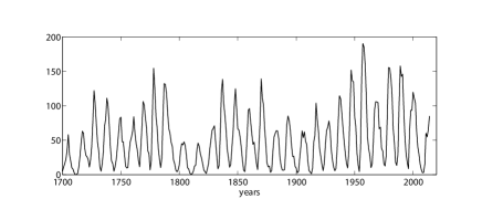
Figure 1: The time series of the annual averaged values of sunspot numbers SSN from 1700 to 2014.

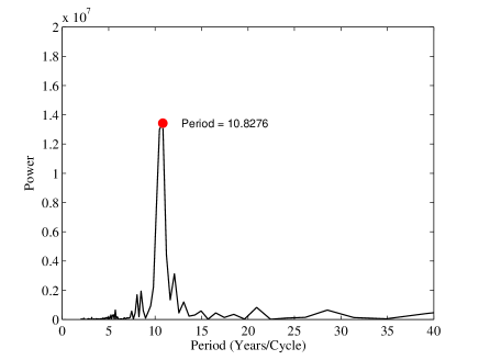
Figure 2: The Fast Fourier Transform of the time series of the annual averaged values of sunspot numbers SSN from 1700 to 2014. The red dot located the precise pick of the strongest frequency.

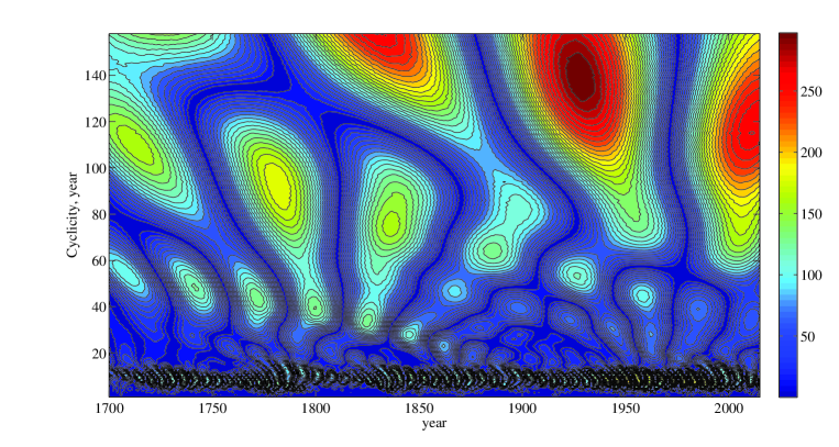
Figure 3: The wavelet image of the time series of the annual averaged values of sunspot numbers SSN from 1700 to 2014 (for wavelet transform calculations we used the Daubechies 10 mother wavelet).

In Figure 1 we can see that the duration of the 11 yr cycle of solar activity ranged from 7 to 17 yrs. The results of observation become more accurate with the beginning of the of direct solar observations (1850–2015).

In Figure 2 we can see how to use Fast Fourier Transform (FFT) method to analyze the variations in sunspot activity (SSN) over the last 300 yr. We can see that the FFT method gives only the value of the duration of the main cycle of magnetic activity of the Sun, which according to the 300-yr observations is equal to 10.83 years. This method does not show cycle’s period evolution: it’s known that according to the last 100-year observations in the XX century, the value of the duration of the main cycle of magnetic activity of the Sun is equal to 10.2 yrs, see [14].

In Figure 3 we illustrated with help of wavelet - analysis the fact that the long time series of observations give us the very useful information for study of the problem of solar flux cyclicity on long time scales. The result of wavelet - analysis (Daubechies wavelet) of series of observations of average annual SSN is presented in form of many of isolines. For the isoline of the value of the wavelet-coefficients are of the same. The maximum values of isolines specify the maximum values of wavelet-coefficients, which corresponds to the most likely value of the period of the cycle. We see there three well-defined cycles of activity: - the main cycle of activity (this cycle is approximately equal to a 10 - 11 yrs), 40-50- yr cyclicity and 100 – 120 yr (ancient) cyclicity.

In Figure 3 we can see that periods of cycles on different time scales are not constant.

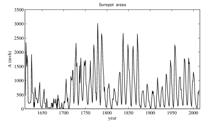
Figure 4: The time series of the annual averaged values of the areas of sunspot numbers A (mvh) from 1610 to 2014.

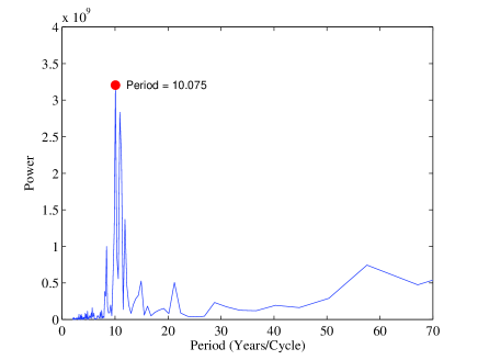
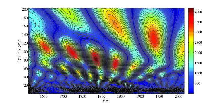
Figure 5: The Fast Fourier Transform of the time series of the annual averaged values of the areas of sunspot numbers A (mvh) from 1610 to 2014. The red dot located the precise pick of the strongest frequency.

Figure 6: The wavelet image of the time series of the annual averaged values of the areas of sunspot numbers A (mvh) from 1610 to 2014 (for wavelet transform calculations we used the Daubechies mother wavelet).

In Figure 4 we can see that the duration of the 11 yr cycle of solar activity according to the annual averaged values of the areas of sunspot numbers A (mvh) from 1610 to 2014 are also ranged from 7 to 17 yrs.

Figure 5 shows the Fast Fourier Transform (FFT) method of analyzing the variations in solar activity according to the annual averaged values of the areas of sunspot numbers A (mvh) over the last 400 year. The FFT gives only the value of the duration of the main cycle of magnetic activity of the Sun, which according to the 400-year observations is equal to 10.075 yrs. This method also does not show cycle’s period evolution.

In Figure 6 we also illustrated with help of wavelet - analysis the fact that the long time series of observations give us the very useful information for study of the problem of solar flux cyclicity on long time scales. The result of wavelet - analysis (Daubechies wavelet) of series of observations of average annual A (mvh) is presented in form of many of isolines. We also can see in Figure 6 three well-defined cycles of activity: - the main cycle of activity (this cycle is approximately equal to a 10 - 11 yrs), 40-50-yr cyclicity and 100 to 120-yr (ancient) cyclicity.

For the wavelet analysis of relative sunspot numbers on the scales in 11 years and quasi-biennial scales we will use the monthly averaged values of SSN, see Figure 7.

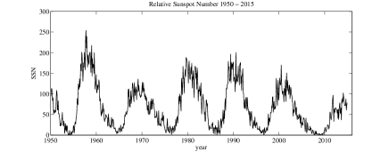
Figure 7: Monthly averaged relative sunspot numbers SSN 1950 - 2015.

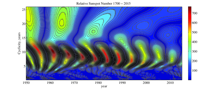
Figure 8: The wavelet image of the cyclic activity of relative sunspot numbers SSN in activity cycles 18 - 24.

The long-term behavior of the sunspot group numbers have been analyzed using wavelet technique by [15] who plotted the changes of the Schwabe cycle (its period is about 11-yr) and studied the grand minima. The temporal evolution of the Gleissberg cycle (its period is about 100-yr) can also be seen in the time-frequency distribution of the solar data. According to [15] the Gleissberg cycle is as variable as the Schwabe cycle. It has two higher amplitude occurrences: first around 1800 (during the Dalton minimum), and then around 1950. They found very interesting fact - the continuous decrease in the frequency (increase of period) of Gleissberg cycle. While near 1750 the cycle length was about 50 yr, it lengthened to approximately 130 yr by 1950.

The study of the indices of solar activity are very important not only for analysis of solar radiation which comes from different altitudes of solar atmosphere. The most important for solar-terrestrial physics is the study of solar radiation influence on the different layers of terrestrial atmosphere (mainly the solar radiation in EUV/UV spectral range which effectively heats the thermosphere of the Earth and so affects to our climate).

In the late of XX century some of solar physicists began to examine with different methods the variations of relative sunspot numbers not only in high amplitude 11-yr Schwabe cycle but in low amplitude cycles approximately equal to half (5.5-yr) and fourth (quasi-biennial) parts of period of the main 11-yr cycle, see [16]. The periods of the quasi-biennial cycles vary considerably within one 11-yr cycle, decreasing from 3.5 to 2 yrs, and this fact complicates the study of such periodicity using the method of periodogram estimates.

Using the methods of frequency analysis of signals the quasi-biennial cycles have been studied not only for the relative sunspot number, but also for 10.7 cm solar radio emission and for some other indices of solar activity, see [17].

It was also shown that the cyclicity on the quasi-biennial time scale takes place often among the stars with 11-yr cyclicity, see [14].

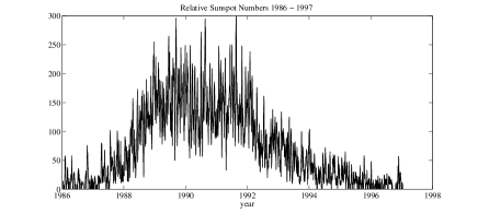
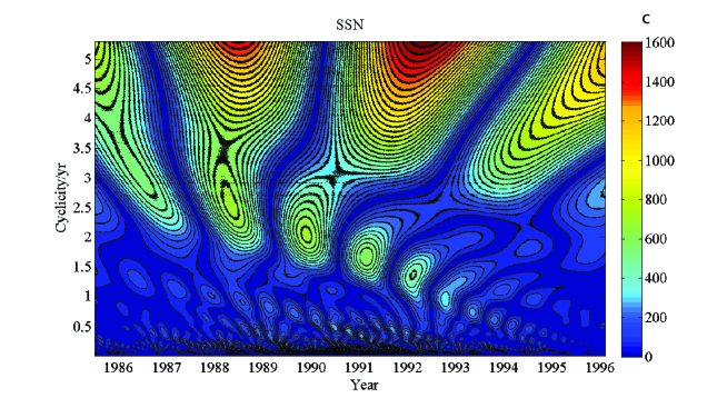
Figure 9: Daily averaged relative sunspot numbers 1986 - 1997.

Figure 10: The wavelet image of the cyclic activity of relative sunspot numbers on the quasi-biennial time scale.

In Figures 6,8 we can see that the periods of cycles on different time scales are not constant too.

Also as in the case of the learning of the Schwabe cycle we see that approximately during three cycles value of the periods decreases (for the Gleissberg cycle from the periods of 110 yrs to 70 yrs, for the Schwabe cycle from the periods of 12 years to 8 years - Figures 3,6). Then during the next cycle there are two equal amplitude cycles (two Gleissberg cycles with periods which change from 130 to 60 yrs - Figure 3, two Schwabe cycles with periods which change from 13 to 7 yrs – Figures 6,8). In the following activity cycle only the cycles with the greatest periods remain and then the value of the periods gradually decreases over the next three cycles.

In Figure 10 we can see that in the case of quasi-biennial cycles the behavior of these periods inside the 11-yr cycle is similar to the variation of cycle’s periods of the Schwabe cycle and the Gleissberg cycle. The periods of quasi-biennial cycles change from 3.5 to 2 yr inside the 11-yr cycle.

For the solar-type F,G and K stars according to Kepler observations it was also found "shorter" chromosphere cycles with periods of about two years, see [18],[19]. In [20] the "shorter" cycle (like solar quasi-biennial) was determined for the star V CVn, it’s duration is equal to 2.7 yr.

3 Observations of magnetic cycles of HK-project stars

The most sensitive indicator of the chromospheric activity (CA) is the Mount Wilson $S$ - index ($S_{HK}$) - the ratio of the core of the CaII H&K lines to the nearby continuum, see [21]. Now the CaII H&K emission was established as the main indicator of CA in lower main sequence stars.

It can be noted that among the databases of observations of Sun-like stars with known values of $S_{HK}$ the sample of stars of the HK-project was selected most carefully in order to study stars which are analogues of the Sun. Moreover, unlike different Planet Search Programs of observations of Sun-like stars, the Mount Wilson Program was specifically developed for a study of a Sun-like cyclical activity of main sequence F, G and K-stars (single) which are the closest to the "young Sun" and "old Sun".

The duration of observations (more than 40 years) in the HK-project has allowed to detect and explore the cyclical activity of the stars, similar to 11-yr cyclical activity of the Sun. First O. Wilson began this program in 1965. He attached great importance to the long-standing systematic observations of cycles in the stars. Fluxes in passbands of 0.1 nm wide and centered on the CaII H&K emission cores have been monitored in 111 stars of the spectral type F2-K5 on or near main sequence on the Hertzsprung-Russell diagram, see [6],[13].

For the HK-project, stars were carefully chosen according to those physical parameters, which are most close to the Sun: cold, single stars – dwarfs, belonging to the main sequence. Close binary systems are excluded.

Results of joint observations of the HK-project radiation fluxes and periods of rotation gave the opportunity for the first time in stellar astrophysics [22] to detect the rotational modulation of the observed fluxes. This meant that on the surface of a star there are inhomogeneities those are living and evolving in several periods of rotation of the stars around its axis. In addition, the evolution of the periods of rotation of the stars in time clearly pointed to the fact of existence of the star’s differential rotations similar to the Sun’s differential rotations.

The authors of the HK-project with use of frequency analysis of the 40-year observations have discovered that the periods of 11-yr cyclic activity vary little in size for the same star from [6],[13]. Durations of cycles vary from 7 to 20 years for different stars. It was shown that stars with cycles represent about 30 % of the total number of studied stars.

The evolution of active regions on a star on a time scale of about 10 years determines the cyclic activity similar to the Sun.

In [6],[13] the regular chromospheric cyclical activity of HK-project Sun-like stars were studied through the analysis of the power spectral density with the Scargle’s periodogram method [23]. It was pointed out that the detection of a periodic signal hidden by a noise is frequently a goal in astronomical data analysis. So, in [6] the periods of HK-project stars activity cycles similar to 11-yr solar activity cycle were determined. The significance of the height of the tallest peak of the periodogram was estimated by the false alarm probability (FAP) function. Among the 50 stars with detected cycles, only 13 stars (with the Sun), which are characterized by the well-determined cyclic activity (the "Excellent" class), have been found.

Unfortunately, the Scargle’s periodogram method (as well as FFT method) allows us only to define a fixed set of main frequencies (that determines the presence of significant periodicities in the series of observations). In the case when the values of periods change significantly during the interval of observations, the accuracy of determination of periods becomes worse. It is also impossible to obtain information about the evolution of the periodicity in time, see [24].

In [20], the different methods, such as Fast Fourier Transform, wavelet analyze, and generalized time-frequency distributions, have been tested and used for analyzing temporal variations in timescales of long-term observational data which have information on the magnetic cycles of active stars and that of the Sun. It was shown that the application of the wavelet analysis is preferable when studying a series of observations of the Sun and stars. Their time-frequency analysis of multi-decadal variability of the solar Schwabe (11-yr) and Gleissberg (century) cycles during the last 250 years showed that one cycle (Schwabe) varies between limits, while the longer one (Gleissberg) continually increases. By analogy from the analysis of the longer solar record, the presence of a long-term trend may suggest an increasing or decreasing of a multi-decadal cycle that is presently unresolved in stellar records of short duration.

A wavelet technique has become popular as a tool for extracting a local time-frequency information. The wavelet transform differs from the traditional time-frequency analysis (Fourier analysis, Scargle’s periodogram method) because of its efficient ability to detect and quantify multi-scale, non-stationary processes, see [15]. The wavelet transform maps a one-dimensional time series $f(t)$ into the two-dimensional plane, related to time and frequency scales. Wavelets are the localized functions which are constructed based on one so-called mother wavelet $\psi(t)$. The choice of wavelet is dictated by signal or image characteristics and the nature of the application. Understanding properties of the wavelet analysis and synthesis, you can choose a mother wavelet function that is optimized for your application.

The standard algorithm of wavelet analysis as applied to astronomical observations of the Sun and stars was discussed in detail in [15], [20]. The choice of the Daubechies and Morlet wavelets as the best mother wavelets $\psi(t)$ for astronomical data processing is discussed in [10],[21] on the basis of comparative analysis of results obtained using different mother wavelets.

The results of our solar data wavelet analysis are presented on the time-frequency plane (Figures 3,6,8,10). The notable crowding of horizontal lines on the time-frequency plane around the specific frequency indicates that the probability of existence of stable cycles is higher for that frequency (cycle’s duration) in accordance with the gradient bar to the right.

In Figures 3,6,8 the results of the continuous wavelet transform analysis (with help of Daubechies mother wavelet) of time series of SSN are presented: Figures 3,6 corresponds to yearly averaged data, Fig 8 corresponds to monthly averaged data, Fig 10 corresponds to daily data. The (X, Y) plane is the time-frequency plane of calculated wavelet-coefficients C(a, b): a-parameter corresponds to Y plane (Cyclicity, years), b-parameter corresponds to X plane (Time, years). The modules of C(a,b) coefficients, characterizing the probability amplitude of regular cyclic component localization exactly at the point (a, b), are laid along the Z axis. In Figure 5 we see the projection of C(a,b) to (a, b) or (X, Y) plane. This projection on the plane (a, b) with isolines allows to trace changes of the coefficients on various scales in time and reveal a picture of local extrema of these surfaces. It is the so-called skeleton of the structure of the analyzed process. We can also note that the configuration of the Morlet and Daubechies wavelets are very compact in frequency, which allows us to determine the localization of instantaneous frequency of observed signal most accurately (compared to other different mother wavelets).

Figures 3,6 confirms the known fact that the period of the main solar activity cycle is about 11-yr in the XIX century and is about 10 yr in the XX century. It is also known that the abnormally long 23-rd cycle of solar activity ended in 2009 and lasted about 12.5 years. Thus, it can be argued that the value of a period of the main cycle of solar activity for past 200 years is not constant and varies by 10 –15 %.

In Figure 10 we show the results of wavelet analysis of daily SSN data in the solar cycle 22. We analyzed that data on the time scale which is equal to several years and identified the second order periodicity such as 5.5 years and quasi-biennial as well as their temporal evolution.

In [25] a study of time variations of cycles of 20 active stars based on decades (long photometric or spectroscopic observations) with a method of time-frequency analysis was done. They found that cycles of sun-like stars show systematic changes. The same phenomenon can be observed for the cycles of the Sun.

In [25] was found that fifteen stars definitely show multiple cycles, the records of the rest are too short to verify a timescale for a second cycle. For 6 HK-project stars (HD 131156A, HD 131156B, HD 100180, HD 201092, HD 201091 and HD 95735) the multiple cycles were detected. Using wavelet analysis the following results (other than periodograms from [6]) were obtained:

HD 131156A shows variability on two time scales: the shorter cycle is about 5.5-yr, a longer-period variability is about 11 yr.

For HD 131156B only one long-term periodicity has been determined.

For HD 100180 the variable cycle of 13.7-yr appears in the beginning of the record; the period decreases to 8.6-yr by the end of the record. The results in the beginning of the dataset are similar to those found by [6], who found two cycles, which are equal to 3.56 and 12.9-yr.

The record for HD 201092 also exhibits two activity cycles: one is equal to 4.7-yr, the other has a time scale of 10-13 years.

The main cycle, seen in the record of HD 201091, has a mean length of 6.7-yr, which slowly changes between 6.2 and 7.2-yr. A shorter, significant cycle is found in the first half of the record with a characteristic time scale of 3.6-yr.

The stronger cycle of HD 95735 is 3.9-yr. A longer, 11-yr cycle is also present with a smaller amplitude.

In our paper we have applied the wavelet analysis for partially available data from the records of relative CaII emission fluxes - the variation of $S_{HK}$ for 1965-1992 observation sets from [6] and for 1985-2002 observations from [13].

We used the detailed plots of $S_{HK}$ time dependencies: each point of the record of observations, which we processed in this paper using wavelet analysis technique, corresponds to three months averaged values of $S_{HK}$.

In this paper we have studied 5 HK-project stars with cyclic activity of the "Excellent" class: HD 10476, HD 81809, HD 103095, HD 152391, HD 160346 and the star HD 185144 with no cyclicity (according [6] classification).

We used the Daubechies 10 wavelet which can most accurately determine the dominant cyclicity as well as its evolution in time in solar data sets at different wavelengths and spectral intervals, see [3].

We hope that wavelet analysis can help to study the temporal evolution of chromospheric cycles of the stars. Tree-month averaging also helps us to avoid the modulation of observational $S_{HK}$ data by star’s rotations.

In Figures 11-22 we present our results for cycles of 6 Mount Wilson HK-project stars.

Figures 11,12 show 3-monthly averaged HD 10476 data set from [6] and [13] plots and the wavelet image of the cyclic activity of HD 10476. We can see that HD 10476 has a mean cycle duration of 10.0-yr in the first half of the record, then it sharply changes to 14-yr, while in [6] was found duration of 9.6-yr. After changing the high amplitude cycle’s period from 10-yr to 14-yr in 1987, the low amplitude cycle remained with 10.0-yr period – we can see two activity cycles. In [6] the duration of HD 10476 mean cycle estimated as 9.6-yr.

Figures 13,14 show 3-monthly averaged HD 81809 data set from [6] and [13] plots and the wavelet image of the cyclic activity of HD 81809. We can see that HD 81809 has a mean cycle duration of 8.2-yr, which slowly changes between 8.3-yr in the first half of the record and 8.1-yr in the middle and the end of the record while in [6] found 8.17-yr.

Figures 15,16 show 3-monthly averaged HD 103095 data set from [6] and [13] plots and the wavelet image of the cyclic activity of HD 103095. HD 103095 has a mean cycle duration of 7.2-yr, which slowly changes between 7.3-yr in the first half of the record, 7.0-yr in the middle and 7.2-yr in the end of the record while in [6] found 7.3-yr.

Figures 17,18 show 3-monthly averaged HD 152391 data set from [6] and [13] plots and the wavelet image of the cyclic activity of HD 152391. HD 152391 has a mean cycle duration of 10.8-yr, which slowly changes between 11.0-yr in the first half of the record and 10.0-yr in the end of the record while in [6] found 10.9-yr.

Figures 19,20 show 3-monthly averaged HD 160346 data set from [6] and [13] plots and the wavelet image of the cyclic activity of HD 160346. HD 160346 has a mean cycle duration of 7.0-yr which does not change during the record in agreement with [6] estimated 7.0-yr.

Figures 21,22 show 3-monthly averaged HD 185144 data set from [6] and [13] plots and the wavelet image of the cyclic activity of HD 185144. HD 185144 has a mean cycle duration of 7-yr which changes between 8-yr in the first half of the record and 6-yr in the end of the record while in [6] haven’t found the well-pronounced cycle.

In [25] the multiple cycles were found for HD 13115A, HD 131156B, HD 93735 stars, for which no cycles have been found in [6]. For the stars of the "Excellent" class HD 201091 and HD 201092, cycle periods found in[6] were confirmed and the shorter cycles (similar to solar quasi-biennial) were also determined.

In [25] have concluded that all the stars from their pattern of cool main sequence stars have cycles and most of the cycle durations change systematically.

However we can see that the stars of the "Excellent" class have relatively constant cycle durations – for these stars the cycle’s periods calculated in [6] and cycle’s periods found with the use of the wavelet analysis are the same.

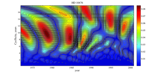
Figure 11: 3-monthly averaged observations of HD 10476 from 1968 to 2002.

Figure 12: The wavelet image of the cyclic activity of HD 10476

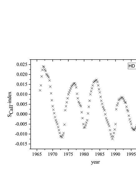
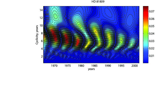
Figure 13: 3-monthly averaged observations of HD 81809 from 1968 to 2002.

Figure 14: The wavelet image of the cyclic activity of HD 81809

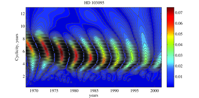
Figure 15: 3-monthly averaged observations of HD 103095 from 1968 to 2002.

Figure 16: The wavelet image of the cyclic activity of HD 103095.

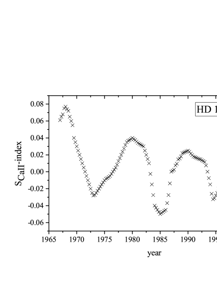
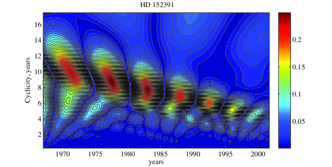
Figure 17: 3-monthly averaged observations of HD 152391 from 1966 to 2002.

Figure 18: The wavelet image of the cyclic activity of HD 152391.

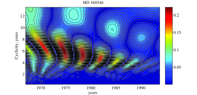
Figure 19: 3-monthly averaged observations of HD 160346 from 1966 to 2002.

Figure 20: The wavelet image of the cyclic activity of HD 160346.

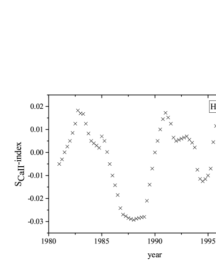
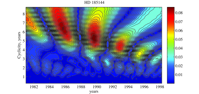
Figure 21: 3-monthly averaged observations of HD 185144 from 1981 to 1999.

Figure 22: The wavelet image of the cyclic activity of HD 185144.

A similar picture can be seen for the Sun: the long-term behavior of the sunspot group numbers has been analyzed using a wavelet technique by [15] who plotted changes of the Schwabe cycle (length and strength) and studied the grand minima. The temporal evolution of the Gleissberg cycle can also be seen in the time-frequency distribution of the solar data. According to [15], the Gleissberg cycle is as variable as the Schwabe cycle. It has two higher amplitude occurrences: the first one is around 1800 (during the Dalton minimum), and the next one is around 1950. They found very interesting fact – the continuous decrease in the frequency (increase of period) of the Gleissberg cycle. While near 1750 the cycle duration was about 50 yr, it lengthened to approximately 130 yr by 1950.

In the late part of the XX century, some of solar physicists began to examine with different methods the variations of relative sunspot numbers not only in the high amplitude 11-yr Schwabe cycle but in low amplitude cycles approximately equal to half (5.5-yr) and fourth (quasi-biennial) parts of the period of the main 11-yr cycle, see [16]. The periods of the quasi-biennial cycles vary considerably within one 11-yr cycle, decreasing from 3.5 to 2 yrs (see Figure 8,10), which complicates a study of such periodicity with the periodogram method.

Using methods of frequency analysis of signals, the quasi-biennial cycles have been studied not only for the relative sunspot number, but also for 10.7 cm solar radio emission and for some other indices of solar activity, see [3]. It was also shown that the cyclicity on the quasi-biennial time scale often takes place among stars with 11-yr cyclicity, see [10,14].

The cyclicity similar to the solar quasi-biennial was also detected for Sun-like stars from direct observations. In [26], the results of direct observations of magnetic cycles of 19 Sun-like stars of F, G, K spectral classes within 4 years were presented. Stars of this sample are characterized by masses between 0.6 and 1.4 of the solar mass and by rotation periods between 3.4 and 43 days. Observations were made using NARVAL spectropolarimeter (Pic du Midi, France) between 2007 and 2011. It was shown that for the stars of this sample $\tau$ Boo and HD 78366 (the same of the Mount Wilson HK-project) the cycle lengths derived by CA by [6] seem to be longer than those derived by spectropolarimetry observations of [26]. They suggest that this apparent discrepancy may be due to the different temporal sampling inherent to these two approaches, so that the sampling adopted at Mount Wilson may not be sufficiently tight to unveil short activity cycles. They hope that future observations of Pic du Midi stellar sample will allow them to investigate longer time scales of the stellar magnetic evolution.

For the Sun-like F, G and K stars according to Kepler observations, "shorter" chromosphere cycles with periods of about two years have also been found, see [18],[19].

We assume that precisely these quasi-biennial cycles were identified in [26]: $\tau$ Boo and HD 78366 are the same of the HK-project, these stars have cycles similar to the quasi-biennial solar cycles with periods of a quarter of the duration of the periods defined in [6].

Note, that in case of the Sun, the amplitude of variations of the radiation in quasi-biennial cycles is substantially less than the amplitude of variations in main 11-yr cycles. We believe that this fact is also true for all Sun-like stars of the HK-project and in the same way for $\tau$ Boo and HD 78366.

The quasi-biennial cycles cannot be detected with the Scargle’s periodogram method. But methods of spectropolarimetry from [26] allowed detecting the cycles with 2 and 3-yr periods. Thus, spectropolarimetry is more accurate method for detection of cycles with different periods and with low amplitudes of variations.

So, the need for wavelet analysis of HK-project observational data is dictated also by the fact that the application of the wavelet method to these observations will help: (1) to find cyclicities with periods equal to a half and a quarter from the main high amplitude cyclicity; (2) to clarify periods of high amplitude cycles and to follow their evolution in time; (3) to find other stars with cycles for which cycles were not determined using the periodogram method due to strong variations of the period as in the case of HD 185144.

4 The parameters of time-evolution study of the cycles

To describe this general trend we propose a formal representation of this process. The cyclic variations of fluxes of solar radiation (in particular, the SSN as the most frequently studied activity index) can be represented by a sinusoid with varying period and constant amplitude:

$$A(t)=cos(2\pi\frac{t-t_{0}}{T})$$

Note that exactly this behavior we can see in different cycles of activity, see Fig.2, Fig.4, Fig.5.

The smooth change of the cycle period can be represented as follows:

$$T(t)=T_{0}-k(t)\cdot(t-t_{0})$$

where $\leavevmode\nobreak\ t_{0}$ is the peak time of the studied cycle, $T_{0}$ is the cycle’s period at the time $t_{0}$, t varies in the range $t_{0}<t<t_{0}+T_{0}$.

Table 1: Parameters of different solar cycles.

Cyclicity	Cycle’s period	k(t)
Solar SSN Century cycle	100 yr	0.3
Solar A(mvh) Two-Century cycle	200 yr	0.3
Solar SSN Half a century cycle	50 yr	0.25
Solar SSN 11-yr cycle	10 -11 yr	0.2
Solar SSN Quasi-biennial cycle	2 - 3.5 yr	0.33
Star’s HD 81809 cycle	6 - 8 yr	0.25
Star’s HD 103095 cycle	5 – 7 yr	0.33
Star’s HD 10476 cycle	10 – 14 yr	0.3
Star’s HD 152391 cycle	8 – 11 yr	0.3
Star’s HD 160346 cycle	5 – 7 yr	0.33
Star’s HD 185144 cycle	5 – 7 yr	0.33

In Table 1. we presented the values of k(t) for different solar cycles. For each solar cycle (from the quasi-biennial duration to 11-yr and 200-yr cycle’s periods) and also for 6 star’s cycles the values of coefficient k(t) are different, see Figures 3,6,8,10,12,14,16,18,20,22. We consider that it is necessary to take into account the temporal evolution of solar and Sun-like star cycles for successful forecasts or the parameters of activity cycles.

5 Conclusions

The study of the evolution of solar cyclicity by observations of the Relative Sunspot Number and Sunspot Areas variation using the wavelet analysis allows us to make more accurate predictions of indices of solar activity (and consequently the predictions of the parameters of the earth’s atmosphere), and also to take a step towards a greater understanding of the nature of cyclicity of solar activity. The close interconnection between activity indices make possible new capabilities in the solar activity indices forecasts. For a long time the scientists were interested in the simulation of processes in the earth’s ionosphere and upper atmosphere. For these purposes it is necessary the successful forecasts of maximum values and other parameters of future activity cycles and also it has been required to take into account the century component.

The study of the evolution of Sun-like stars cyclicity by example of Mount Wilson observations of $S_{HK}$ - index using the wavelet analysis reveals the similar features in solar and stellar cyclic activity: the existence of multiple cycles and their evolution in time.

Wavelet analysis of these data reveals the following features: the period and phase of these relatively low frequency variations of the solar or stellar fluxes, previous to the studied time point, influence to the amplitudes and to the phase of studied time point. Solar or stellar fluxes show the gradually changing of their values in time: as a result, the periods of variations are getting longer.

References

- [1] Svalgaard, L., Lockwood, M., Beer, J. 2011, http://www.leif.org/research/Svalgaard_ISSI_Proposal_Base.pdf.
- [2] Svalgaard, L., Cliver, E.W. 2010, J. Geophys. Res., 115, A09111.
- [3] Bruevich, E.A. and Yakunina, G.V. 2015, Moscow University Physics Bulletin, 70, Issue 4, 282.
- [4] Bruevich, E.A., Alekseev, I.Yu. 2007, Astrophysics, 50, Issue 2, 187.
- [5] Bruevich, E.A., Katsova, M.M. and Sokolov, D.D. 2001, Astronomy Reports, 45, Issue 9, 716.
- [6] Baliunas, S.L., Donahue, R.A. et al. 1995, ApJ, 438, 269.
- [7] Wright, J.T., Marcy, G.W., Butler, R.P., Vogt, S.S., 2004. ApJS, 152, Issue 2, 261.
- [8] Arriagada, P. 2011, ApJ, 734, 70.
- [9] Bruevich, E.A., Bruevich, V.V., Shimanovskaya, E.V. 2016, Astrophysics, 59, Issue 1, 101.
- [10] Shimanovskaya, E.V, Bruevich, V.V., Bruevich, E.A. 2016, Research in Astronomy and Astrophysics, 16, Issue 9, 148.
- [11] Nagovitsyn, Yu.A., Tlatov, A.G., Nagovitsyna E.Yu. 2016, Astronomy Reports, 60, Issue 9, 831.
- [12] National Geophysical Data Center Solar and Terrestrial Physics. 2016, http://www.ngdc.noaa.gov/stp/solar/solardataservices.html.
- [13] Lockwood, G.W., Skif, B.A., Radick, R.R., Baliunas, S.L., Donahue, R.A. and Soon, W. 2007, ApJS, 171, 260.
- [14] Bruevich, E.A. and Kononovich, E.V. 2011, Moscow University Physics Bulletin, 66, Issue 1, 72.
- [15] Frick, P., Baliunas, S.L., Galyagin, D., Sokoloff, D. and Soon, W. 1997, ApJ, 483, 426.
- [16] Vitinsky, Yu., Kopezky, M., Kuklin G., 1986. The sunspot solar activity statistic. M. Nauka
- [17] Bruevich, E.A., Bruevich, V.V., Yakunina, G.V. 2014, J. Astrophys. Astron., 35, 1.
- [18] Metcalfe, T.S., Monteiro, M. et al. 2010, ApJ, 723, 1583.
- [19] Garcia, R.A., Mathur, S. et al. 2010, Science, 329, 1032.
- [20] Kollath, Z. and Olah, K. 2009, Astron. and Astrophys., 501, 695.
- [21] Vaugan, A.H., Preston, G.W. 1980, PASP, 92, 385.
- [22] Noyes, R.W., Hartman, L., Baliunas, S.L., Duncan, D.K., Vaugan, A.H. and Parker, E.N. 1984, ApJ, 279, 763.
- [23] Scargle, J.D. 1982, ApJ, 263, 835.
- [24] Bruevich, E.A., Bruevich, V.V. and Yakunina, G.V. 2014, Sun and Geosphere, 8, 91.
- [25] Olah, K., Kollath, Z., Granzer, T. et al. 2009, Astron. and Astrophys., 501, 703.
- [26] Morgenthaler, A., Petit, P., Morin, J., Auriere, M., Dintrans, B., Konstantinova-Antova, R., Marsden S. 2011, Astron. Nachr., 332, 866.