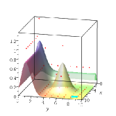
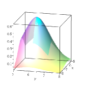
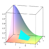
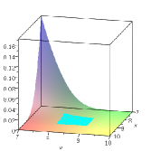
b-Spline Curves and Surfaces as a Minimization of Quadratic Operators

Svetoslav I. Nenov Department of Mathematics, University of Chemical Technology and Metallurgy, Sofia 1756, Bulgaria nenov@uctm.edu
Abstract.

The goal of this short note is to prove that every b-spline curve or surface (generated by uniform knots, without multiplicity) may be defined as minimum of positive quadratic operator.

1. Introduction

The b-spline curves and surfaces are an essential tool in many engineering software for design and visualization – for example ANSYS, RFEM 3D, etc. So, it is necessary to have in these applications many different methods to construct b-spline elements. Also see [11], [12], and references therein.

We will prove that any b-spline curve or surface minimizes positive quadratic operator: appropriate moving least-square error.

Let us mark that different approaches in moving least-squares method are used by Shepard – computer software SYMAP (Harvard Laboratory for Computer Graphics), Lancaster in 1979, and the works of D. Levin in 1999, see [8]. In [10] it has been shown that moving least-squares method is an adequate mathematical tool for determining diesel-fuel cetane-number (or cetane-index) from easily available physical properties of fuels.

In this section we will remind the definition of b-splines generated by control points in d+1superscript𝑑1{\mathbb{R}}^{d+1} and definition of moving least-squares approximation for a given data set {(𝒙i,f(𝒙i)):𝒙id}d+1conditional-setsubscript𝒙𝑖𝑓subscript𝒙𝑖subscript𝒙𝑖superscript𝑑superscript𝑑1\{(\boldsymbol{x}_{i},f(\boldsymbol{x}_{i})):\boldsymbol{x}_{i}\in{\mathbb{R}}^{d}\}\subset{\mathbb{R}}^{d+1}.

2. Preliminaries

2.1. b-Splines

Let {𝒑id+1:i=0,,n}conditional-setsubscript𝒑𝑖superscript𝑑1𝑖0𝑛\{\boldsymbol{p}_{i}\in{\mathbb{R}}^{d+1}:i=0,\dots,n\} be a set of n+1𝑛1n+1 (control) points.

Let r𝑟r be an integer, 1rn+11𝑟𝑛11\leq r\leq n+1 (the order of spline).

We will use uniform knots, without multiplicity: ti=isubscript𝑡𝑖𝑖t_{i}=i, i=0,,n+r𝑖0𝑛𝑟i=0,\dots,n+r.

Using Cox-de Boor recursion formula (see [3], [4]), let us define the following basis functions:

Bi,1(t)={1,iftit<ti+1,0,otherwise,subscript𝐵𝑖1𝑡cases1ifsubscript𝑡𝑖𝑡subscript𝑡𝑖10otherwise\displaystyle B_{i,1}(t)=\begin{cases}1,&\quad\text{if}\ t_{i}\leq t<t_{i+1},\\ 0,&\quad\text{otherwise},\end{cases} (1)

for 0in+r10𝑖𝑛𝑟10\leq i\leq n+r-1; and

Bi,j(t)=ttiti+j1tiBi,j1(t)+ti+jtti+jti+1Bi+1,j1(t)=tij1Bi,j1(t)+i+jtj1Bi+1,j1(t),subscript𝐵𝑖𝑗𝑡𝑡subscript𝑡𝑖subscript𝑡𝑖𝑗1subscript𝑡𝑖subscript𝐵𝑖𝑗1𝑡subscript𝑡𝑖𝑗𝑡subscript𝑡𝑖𝑗subscript𝑡𝑖1subscript𝐵𝑖1𝑗1𝑡𝑡𝑖𝑗1subscript𝐵𝑖𝑗1𝑡𝑖𝑗𝑡𝑗1subscript𝐵𝑖1𝑗1𝑡\displaystyle\begin{split}B_{i,j}(t)=&\dfrac{t-t_{i}}{t_{i+j-1}-t_{i}}B_{i,j-1}(t)+\dfrac{t_{i+j}-t}{t_{i+j}-t_{i+1}}B_{i+1,j-1}(t)\\ =&\dfrac{t-i}{j-1}B_{i,j-1}(t)+\dfrac{i+j-t}{j-1}B_{i+1,j-1}(t),\end{split} (2)

for 2jr2𝑗𝑟2\leq j\leq r, 0in+rj0𝑖𝑛𝑟𝑗0\leq i\leq n+r-j.

The b-spline curve of order r𝑟r is defined as a linear combination of control points 𝒑isubscript𝒑𝑖\boldsymbol{p}_{i}:

𝜸(t)=i=0nBi,r(t)𝒑i,t[tr1,tn+1].formulae-sequence𝜸𝑡superscriptsubscript𝑖0𝑛subscript𝐵𝑖𝑟𝑡subscript𝒑𝑖𝑡subscript𝑡𝑟1subscript𝑡𝑛1\displaystyle\boldsymbol{\gamma}(t)=\sum\limits_{i=0}^{n}B_{i,r}(t)\boldsymbol{p}_{i},\quad t\in[t_{r-1},t_{n+1}]. (3)

2.2. Moving Least-Squares Method

Let:

  1. (1)

    𝒟𝒟\mathcal{D} be a bounded domain in dsuperscript𝑑\mathbb{R}^{d}.

  2. (2)

    𝒙i𝒟subscript𝒙𝑖𝒟\boldsymbol{x}_{i}\in\mathcal{D}, i=0,,m𝑖0𝑚i=0,\dots,m; 𝒙i𝒙jsubscript𝒙𝑖subscript𝒙𝑗\boldsymbol{x}_{i}\not=\boldsymbol{x}_{j}, if ij𝑖𝑗i\not=j.

  3. (3)

    f:𝒟:𝑓𝒟f:\mathcal{D}\to\mathbb{R} be a continuous function.

  4. (4)

    pi:𝒟:subscript𝑝𝑖𝒟p_{i}:\mathcal{D}\to\mathbb{R} be continuous functions, i=1,,l𝑖1𝑙i=1,\dots,l. The functions {p1,,pl}subscript𝑝1subscript𝑝𝑙\{p_{1},\dots,p_{l}\} are linearly independent in 𝒟𝒟\mathcal{D} and let 𝒫lsubscript𝒫𝑙\mathcal{P}_{l} be their linear span.

  5. (5)

    W:(0,)(0,):𝑊00W:(0,\infty)\to(0,\infty) is a strictly positive functions.

Usually the basis in 𝒫lsubscript𝒫𝑙\mathcal{P}_{l} is constructed by monomials. For example: pl(𝒙)=x1k1xdkdsubscript𝑝𝑙𝒙superscriptsubscript𝑥1subscript𝑘1superscriptsubscript𝑥𝑑subscript𝑘𝑑p_{l}(\boldsymbol{x})=x_{1}^{k_{1}}\dots x_{d}^{k_{d}}, where 𝒙=(x1,,xd)𝒙subscript𝑥1subscript𝑥𝑑\boldsymbol{x}=(x_{1},\dots,x_{d}), k1,kdsubscript𝑘1subscript𝑘𝑑k_{1},\dots k_{d}\in\mathbb{N}, k1++kdl1subscript𝑘1subscript𝑘𝑑𝑙1k_{1}+\dots+k_{d}\leq l-1. In the case d=1𝑑1d=1, the standard basis is {1,x,,xl1}1𝑥superscript𝑥𝑙1\{1,x,\dots,x^{l-1}\}.

Following [5], [6], [7], [8], we use the following definition. The moving least-squares approximation of order l𝑙l at a fixed point 𝒙𝒙\boldsymbol{x} is the value of p(𝒙)superscript𝑝𝒙p^{*}(\boldsymbol{x}), where p𝒫lsuperscript𝑝subscript𝒫𝑙p^{*}\in\mathcal{P}_{l} is minimizing the least-squares error

i=1mW(𝒙𝒙i)(p(𝒙)f(𝒙i))2superscriptsubscript𝑖1𝑚𝑊norm𝒙subscript𝒙𝑖superscript𝑝𝒙𝑓subscript𝒙𝑖2\displaystyle\sum_{i=1}^{m}W(\|\boldsymbol{x}-\boldsymbol{x}_{i}\|)\left(p(\boldsymbol{x})-f(\boldsymbol{x}_{i})\right)^{2} (4)

among all p𝒫l𝑝subscript𝒫𝑙p\in\mathcal{P}_{l}.

The approximation is “local” if weight function W(s)𝑊𝑠W(s) is fast decreasing as s𝑠s tends to infinity. Interpolation is achieved if W(0)=𝑊0W(0)=\infty. We define additional function w:[0,)[0,):𝑤00w:[0,\infty)\to[0,\infty), such taht:

w(s)={1W(s),if (s>0) or (s=0 and W(0)<),0,if (s=0 and W(0)=).𝑤𝑠cases1𝑊𝑠if (s>0) or (s=0 and W(0)<)0if (s=0 and W(0)=)w(s)=\begin{cases}\dfrac{1}{W(s)},&\quad\text{if ($s>0$) or ($s=0$ and $W(0)<\infty$)},\\ 0,&\quad\text{if ($s=0$ and $W(0)=\infty$)}.\end{cases}

Some examples of W(s)𝑊𝑠W(s) and w(s)𝑤𝑠w(s), s0𝑠0s\geq 0:

W(s)=eα2s2𝑊𝑠superscript𝑒superscript𝛼2superscript𝑠2\displaystyle W(s)=e^{-\alpha^{2}s^{2}} exp-weight,exp-weight\displaystyle\qquad\text{$\exp$-weight},
W(s)=sα2𝑊𝑠superscript𝑠superscript𝛼2\displaystyle W(s)=s^{-\alpha^{2}} Shepard weights,Shepard weights\displaystyle\qquad\text{Shepard weights},
w(s)=s2eα2s2𝑤𝑠superscript𝑠2superscript𝑒superscript𝛼2superscript𝑠2\displaystyle w(s)=s^{2}e^{-\alpha^{2}s^{2}} McLain weight,McLain weight\displaystyle\qquad\text{McLain weight},
w(s)=eα2s21𝑤𝑠superscript𝑒superscript𝛼2superscript𝑠21\displaystyle w(s)=e^{\alpha^{2}s^{2}}-1 see Levin’s works.see Levin’s works\displaystyle\qquad\text{see Levin's works}.

Here and below: the superscript t denotes transpose of matrix; I𝐼I is the identity matrix.

Let us introduce the matrices:

E=𝐸absent\displaystyle E= (p1(𝒙1)p2(𝒙1)pl(𝒙1)p1(𝒙2)p2(𝒙2)pl(𝒙2)p1(𝒙m)p2(𝒙m)pl(𝒙m)),𝒂=(a1a2am),𝒄=(p1(𝒙)p2(𝒙)pl(𝒙))formulae-sequencematrixsubscript𝑝1subscript𝒙1subscript𝑝2subscript𝒙1subscript𝑝𝑙subscript𝒙1subscript𝑝1subscript𝒙2subscript𝑝2subscript𝒙2subscript𝑝𝑙subscript𝒙2missing-subexpressionsubscript𝑝1subscript𝒙𝑚subscript𝑝2subscript𝒙𝑚subscript𝑝𝑙subscript𝒙𝑚𝒂matrixsubscript𝑎1subscript𝑎2subscript𝑎𝑚𝒄matrixsubscript𝑝1𝒙subscript𝑝2𝒙subscript𝑝𝑙𝒙\displaystyle\begin{pmatrix}p_{1}(\boldsymbol{x}_{1})&p_{2}(\boldsymbol{x}_{1})&\cdots&p_{l}(\boldsymbol{x}_{1})\\ p_{1}(\boldsymbol{x}_{2})&p_{2}(\boldsymbol{x}_{2})&\cdots&p_{l}(\boldsymbol{x}_{2})\\ \vdots&\vdots&&\vdots\\ p_{1}(\boldsymbol{x}_{m})&p_{2}(\boldsymbol{x}_{m})&\cdots&p_{l}(\boldsymbol{x}_{m})\\ \end{pmatrix},\ \boldsymbol{a}=\begin{pmatrix}a_{1}\\ a_{2}\\ \vdots\\ a_{m}\end{pmatrix},\ \boldsymbol{c}=\begin{pmatrix}p_{1}(\boldsymbol{x})\\ p_{2}(\boldsymbol{x})\\ \vdots\\ p_{l}(\boldsymbol{x})\end{pmatrix}
D=𝐷absent\displaystyle D= 2(w(𝒙𝒙1)000w(𝒙𝒙2)000w(𝒙𝒙m)).2matrix𝑤norm𝒙subscript𝒙1000𝑤norm𝒙subscript𝒙20missing-subexpression00𝑤norm𝒙subscript𝒙𝑚\displaystyle 2\begin{pmatrix}w(\|\boldsymbol{x}-\boldsymbol{x}_{1}\|)&0&\cdots&0\\ 0&w(\|\boldsymbol{x}-\boldsymbol{x}_{2}\|)&\cdots&0\\ \vdots&\vdots&&\vdots\\ 0&0&\cdots&w(\|\boldsymbol{x}-\boldsymbol{x}_{m}\|)\\ \end{pmatrix}.

Through the article, we assume the following conditions (H1):

  1. (H1.1)

    1𝒫l1subscript𝒫𝑙1\in\mathcal{P}_{l}.

  2. (H1.2)

    1lm1𝑙𝑚1\leq l\leq m.

  3. (H1.3)

    rank(Et)=lsuperscript𝐸𝑡𝑙(E^{t})=l.

  4. (H1.4)

    w𝑤w is a smooth function.

Theorem 2.1 (see [6]).

Let the conditions (H1) hold true.

Then:

  1. (1)

    The matrix EtD1Esuperscript𝐸𝑡superscript𝐷1𝐸E^{t}D^{-1}E is non-singular.

  2. (2)

    The approximation defined by the moving least-squares method is

    L^(f)=i=1maif(𝒙i),^𝐿𝑓superscriptsubscript𝑖1𝑚subscript𝑎𝑖𝑓subscript𝒙𝑖\displaystyle\hat{L}(f)=\sum_{i=1}^{m}a_{i}f(\boldsymbol{x}_{i}), (5)

    where

    𝒂=A0𝒄andA0=D1E(EtD1E)1.formulae-sequence𝒂subscript𝐴0𝒄andsubscript𝐴0superscript𝐷1𝐸superscriptsuperscript𝐸𝑡superscript𝐷1𝐸1\displaystyle\boldsymbol{a}=A_{0}\boldsymbol{c}\quad\text{and}\quad A_{0}=D^{-1}E\left(E^{t}D^{-1}E\right)^{-1}. (6)
  3. (3)

    If w(0)=0𝑤00w(0)=0, then the approximation is interpolatory.

3. b-Spline Curve as a Minimum of
Moving Least-Squares Error

Using the definitions and notations introduced in Section 2, our goal is to prove the following theorem.

Theorem 3.1.

Let:

  1. (1)

    d=1𝑑1d=1, n,r+𝑛𝑟subscriptn,r\in{\mathbb{Z}_{+}}, rn+1𝑟𝑛1r\leq n+1, f:[0,n+r]:𝑓0𝑛𝑟f:[0,n+r]\to\mathbb{R} be a continuous function.

  2. (2)

    𝒑i=(i,f(i))subscript𝒑𝑖𝑖𝑓𝑖\boldsymbol{p}_{i}=(i,f(i)), i=0,,n+r𝑖0𝑛𝑟i=0,\dots,n+r.

  3. (3)

    Let 𝜸(t)=(γ1(t)γ2(t))𝜸𝑡subscript𝛾1𝑡subscript𝛾2𝑡\boldsymbol{\gamma}(t)=\left(\begin{smallmatrix}\gamma_{1}(t)\\ \gamma_{2}(t)\end{smallmatrix}\right) be the b-spline of order r𝑟r and knot vector {ti=i:i=0,,n+r}conditional-setsubscript𝑡𝑖𝑖𝑖0𝑛𝑟\{t_{i}=i:i=0,\dots,n+r\}.

Then γ1(t)=t2subscript𝛾1𝑡𝑡2\gamma_{1}(t)=t-2, t[0,n+r]𝑡0𝑛𝑟t\in[0,n+r] and there exists a weight function W𝑊W, such that

γ2(x)=L^(f)(x),x[r1,n+1],formulae-sequencesubscript𝛾2𝑥^𝐿𝑓𝑥𝑥𝑟1𝑛1\gamma_{2}(x)=\hat{L}(f)(x),\quad x\in[r-1,n+1],

where L^(f)(x)^𝐿𝑓𝑥\hat{L}(f)(x) is the approximation defined by the moving least-squares method for the data {𝐩i:i=0,,n+r}conditional-setsubscript𝐩𝑖𝑖0𝑛𝑟\{\boldsymbol{p}_{i}:i=0,\dots,n+r\}.

Proof.

We will prove the theorem for the cubic splines, i.e. r=4𝑟4r=4. The proof for the different orders is similar.

From conditions (2) and (3), if we set xi=isubscript𝑥𝑖𝑖x_{i}=i, then ti=xisubscript𝑡𝑖subscript𝑥𝑖t_{i}=x_{i}, i=0,,n𝑖0𝑛i=0,\dots,n and hence γ1(t)=tsubscript𝛾1𝑡𝑡\gamma_{1}(t)=t.

The b-spline curve of order 444, defined using knots {ti=i:i=0,,n+r}conditional-setsubscript𝑡𝑖𝑖𝑖0𝑛𝑟\{t_{i}=i:i=0,\dots,n+r\}, is

γ2(t)=i=0nBi,4(t)f(xi),x[tr1,tn+1][3,n+1].formulae-sequencesubscript𝛾2𝑡superscriptsubscript𝑖0𝑛subscript𝐵𝑖4𝑡𝑓subscript𝑥𝑖𝑥subscript𝑡𝑟1subscript𝑡𝑛13𝑛1\gamma_{2}(t)=\sum\limits_{i=0}^{n}B_{i,4}(t)f(x_{i}),\quad x\in[t_{r-1},t_{n+1}]\equiv[3,n+1].
\vdots \vdots
ti02<ti01subscript𝑡subscript𝑖02subscript𝑡subscript𝑖01t_{i_{0}-2}<t_{i_{0}-1}: Bi02,1(t)=0subscript𝐵subscript𝑖021𝑡0B_{i_{0}-2,1}(t)=0
Bi02,2(t)=0subscript𝐵subscript𝑖022𝑡0B_{i_{0}-2,2}(t)=0
ti01<ti0subscript𝑡subscript𝑖01subscript𝑡subscript𝑖0t_{i_{0}-1}<t_{i_{0}}: Bi01,1(t)=0subscript𝐵subscript𝑖011𝑡0B_{i_{0}-1,1}(t)=0 Bi02,3(t)>0subscript𝐵subscript𝑖023𝑡0B_{i_{0}-2,3}(t)>0
Bi01,2(t)>0subscript𝐵subscript𝑖012𝑡0B_{i_{0}-1,2}(t)>0 Bi02,4(t)>0subscript𝐵subscript𝑖024𝑡0B_{i_{0}-2,4}(t)>0\vdots
ti0<t<ti0+1subscript𝑡subscript𝑖0𝑡subscript𝑡subscript𝑖01t_{i_{0}}<t<t_{i_{0}+1}: Bi0,1(t)=1subscript𝐵subscript𝑖01𝑡1B_{i_{0},1}(t)=1 Bi01,3(t)>0subscript𝐵subscript𝑖013𝑡0B_{i_{0}-1,3}(t)>0
Bi0,2(t)>0subscript𝐵subscript𝑖02𝑡0B_{i_{0},2}(t)>0 Bi01,4(t)>0subscript𝐵subscript𝑖014𝑡0B_{i_{0}-1,4}(t)>0\vdots
ti0+1<ti0+2subscript𝑡subscript𝑖01subscript𝑡subscript𝑖02t_{i_{0}+1}<t_{i_{0}+2}: Bi0+1,1(t)=0subscript𝐵subscript𝑖011𝑡0B_{i_{0}+1,1}(t)=0 Bi0,3(t)>0subscript𝐵subscript𝑖03𝑡0B_{i_{0},3}(t)>0
Bi0+1,2(t)=0subscript𝐵subscript𝑖012𝑡0B_{i_{0}+1,2}(t)=0
ti0+2<ti0+3subscript𝑡subscript𝑖02subscript𝑡subscript𝑖03t_{i_{0}+2}<t_{i_{0}+3}: Bi0+2,1(t)=0subscript𝐵subscript𝑖021𝑡0B_{i_{0}+2,1}(t)=0
\vdots \vdots

Table 1. Cox-de Boor recursion algorithm

The following properties of b-spline basis functions Bi,j(t)subscript𝐵𝑖𝑗𝑡B_{i,j}(t) are well known:

  1. (BS-0)

    By the direc calculation (see formulas (1), (2), and the schema illustrated in Table 1, r=4𝑟4r=4):

    Bi,4(t)={0,ift<i,16(ti)3,ifit<i+1,23(ti1)3+16(ti)3,ifi+1t<i+2,(ti2)323(ti1)3+16(ti)3,ifi+2t<i+3,23(ti3)3+(ti2)323(ti1)3+16(ti)3,ifi+3t<i+4,0,ifi+4t.subscript𝐵𝑖4𝑡cases0if𝑡𝑖16superscript𝑡𝑖3if𝑖𝑡𝑖123superscript𝑡𝑖1316superscript𝑡𝑖3if𝑖1𝑡𝑖2superscript𝑡𝑖2323superscript𝑡𝑖13otherwise16superscript𝑡𝑖3if𝑖2𝑡𝑖323superscript𝑡𝑖33superscript𝑡𝑖23otherwise23superscript𝑡𝑖1316superscript𝑡𝑖3if𝑖3𝑡𝑖40if𝑖4𝑡\displaystyle B_{i,4}(t)=\begin{cases}0,&\ \text{if}\ t<i,\\[4.0pt] \dfrac{1}{6}\left(t-i\right)^{3},&\ \text{if}\ i\leq t<i+1,\\[4.0pt] -\dfrac{2}{3}\left(t-i-1\right)^{3}+\dfrac{1}{6}\left(t-i\right)^{3},&\ \text{if}\ i+1\leq t<i+2,\\[4.0pt] \left(t-i-2\right)^{3}-\dfrac{2}{3}\left(t-i-1\right)^{3}&\\[4.0pt] +\dfrac{1}{6}\left(t-i\right)^{3},&\ \text{if}\ i+2\leq t<i+3,\\[4.0pt] -\dfrac{2}{3}\left(t-i-3\right)^{3}+\left(t-i-2\right)^{3}&\\[4.0pt] -\dfrac{2}{3}\left(t-i-1\right)^{3}+\dfrac{1}{6}\left(t-i\right)^{3},&\ \text{if}\ i+3\leq t<i+4,\\[4.0pt] 0,&\ \text{if}\ i+4\leq t.\end{cases}
  2. (BS-1)

    If t(i,i+j)𝑡𝑖𝑖𝑗t\in(i,i+j), then Bi,j(t)>0subscript𝐵𝑖𝑗𝑡0B_{i,j}(t)>0.

  3. (BS-2)

    If t[0,i][i+j,n+j]𝑡0𝑖𝑖𝑗𝑛𝑗t\in[0,i]\cup[i+j,n+j], then Bi,j(t)=0subscript𝐵𝑖𝑗𝑡0B_{i,j}(t)=0.

  4. (BS-3)

    i=0nBi,j(t)=1superscriptsubscript𝑖0𝑛subscript𝐵𝑖𝑗𝑡1\sum\limits_{i=0}^{n}B_{i,j}(t)=1, for any t(j1,n+1)𝑡𝑗1𝑛1t\in(j-1,n+1).

  5. (BS-4)

    Bi,j(t)subscript𝐵𝑖𝑗𝑡B_{i,j}(t) has Cj2superscript𝐶𝑗2C^{j-2} continuity at each knot.

  6. (BS-5)

    By the simple substitutions in the formulas in (BS-0):

    Bi,j(t+i)=subscript𝐵𝑖𝑗𝑡𝑖absent\displaystyle B_{i,j}(t+i)= Bk,j(t+k),subscript𝐵𝑘𝑗𝑡𝑘\displaystyle B_{k,j}(t+k), t(0,j),𝑡0𝑗\displaystyle t\in(0,j),
    Bi2,j(t)=subscript𝐵𝑖2𝑗𝑡absent\displaystyle B_{i-2,j}(t)= Bi,j(t+2),subscript𝐵𝑖𝑗𝑡2\displaystyle B_{i,j}(t+2),\qquad t(i2,i+j2).𝑡𝑖2𝑖𝑗2\displaystyle t\in(i-2,i+j-2).

Let t𝑡t be a fixed point in the interval (3,n+1)3𝑛1(3,n+1) and i0subscript𝑖0i_{0} be an integer such taht 3i0<t<i0+1n+13subscript𝑖0𝑡subscript𝑖01𝑛13\leq i_{0}<t<i_{0}+1\leq n+1. Then

γ2(t)=i=0nBi,4(t)f(i)=i=i03i0Bi,4(t)f(i).subscript𝛾2𝑡superscriptsubscript𝑖0𝑛subscript𝐵𝑖4𝑡𝑓𝑖superscriptsubscript𝑖subscript𝑖03subscript𝑖0subscript𝐵𝑖4𝑡𝑓𝑖\displaystyle\gamma_{2}(t)=\sum\limits_{i=0}^{n}B_{i,4}(t)f(i)=\sum\limits_{i=i_{0}-3}^{i_{0}}B_{i,4}(t)f(i). (7)

because if i=1,,i04,i0+1,,n𝑖1subscript𝑖04subscript𝑖01𝑛i=1,\dots,i_{0}-4,i_{0}+1,\dots,n, then Bi,4(x)=0subscript𝐵𝑖4𝑥0B_{i,4}(x)=0, see (BS-1) and (BS-2).

On the other hand, let us consider the moving least-squares problem for the given data {(i,f(i)):i=0,,n+4}conditional-set𝑖𝑓𝑖𝑖0𝑛4\{(i,f(i)):i=0,\dots,n+4\}. Let us set l=1𝑙1l=1, and

W(x)={0,ifx<2,16(x+2)3,if2x<1,12x3x2+23,if1x<0,12x3x2+23,if 0x<1,16(x2)3,if 1x<2,0,if 2x,𝑊𝑥cases0if𝑥216superscript𝑥23if2𝑥112superscript𝑥3superscript𝑥223if1𝑥012superscript𝑥3superscript𝑥223if 0𝑥116superscript𝑥23if1𝑥20if2𝑥\displaystyle W(x)=\begin{cases}0,&\ \text{if}\ x<-2,\\[4.0pt] \dfrac{1}{6}(x+2)^{3},&\ \text{if}\ -2\leq x<-1,\\[4.0pt] -\dfrac{1}{2}x^{3}-x^{2}+\dfrac{2}{3},&\ \text{if}\ -1\leq x<0,\\[4.0pt] \dfrac{1}{2}x^{3}-x^{2}+\dfrac{2}{3},&\ \text{if}\ 0\leq x<1,\\[4.0pt] -\dfrac{1}{6}(x-2)^{3},&\ \text{if}\ 1\leq x<2,\\[4.0pt] 0,&\ \text{if}\ 2\leq x,\end{cases}

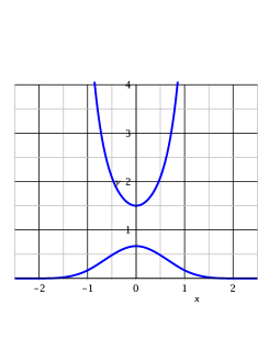
see Figure 1.

Refer to caption

Figure 1. The graphics of W(x),x(2.5,2.5)𝑊𝑥𝑥2.52.5W(x),\ x\in(-2.5,2.5) and w(x),x(1,1)𝑤𝑥𝑥11w(x),\ x\in(-1,1)

Then for any i=0,,n𝑖0𝑛i=0,\dots,n, we have (see also (BS-5)):

W(|x|)=W(x)=Bi,4(x+i+2)=Bi2,4(x+i),x[2,2].formulae-sequence𝑊𝑥𝑊𝑥subscript𝐵𝑖4𝑥𝑖2subscript𝐵𝑖24𝑥𝑖𝑥22W(|x|)=W(x)=B_{i,4}(x+i+2)=B_{i-2,4}(x+i),\quad x\in[-2,2].

Hence W(|xi|)=Bi2,4(x)𝑊𝑥𝑖subscript𝐵𝑖24𝑥W(|x-i|)=B_{i-2,4}(x), x[i2,i+2]𝑥𝑖2𝑖2x\in[i-2,i+2].

The least-squares error is (see also conditions (H1): p1(x)=1subscript𝑝1𝑥1p_{1}(x)=1, so p(x)=p𝑝𝑥𝑝p(x)=p has to be a constant)

i=1n+rW(xi)(pf(i))2=i=i01i0+2W(xi)(pf(i))2,superscriptsubscript𝑖1𝑛𝑟𝑊𝑥𝑖superscript𝑝𝑓𝑖2superscriptsubscript𝑖subscript𝑖01subscript𝑖02𝑊𝑥𝑖superscript𝑝𝑓𝑖2\sum_{i=1}^{n+r}W(x-i)\left(p-f(i)\right)^{2}=\sum_{i=i_{0}-1}^{i_{0}+2}W(x-i)\left(p-f(i)\right)^{2},

because W(xi)>0𝑊𝑥𝑖0W(x-i)>0, iff i01ii0+2subscript𝑖01𝑖subscript𝑖02i_{0}-1\leq i\leq i_{0}+2.

It is not hard to compute

E=𝐸absent\displaystyle E= (1111),𝒄=(1),matrix1111𝒄matrix1\displaystyle\begin{pmatrix}1\\ 1\\ 1\\ 1\\ \end{pmatrix},\ \boldsymbol{c}=\begin{pmatrix}1\end{pmatrix},
D=𝐷absent\displaystyle D= 2(w(|x(i01)|)0000w(|xi0|)0000w(|x(i0+1)|)0000w(|x(i0+2)|)),2matrix𝑤𝑥subscript𝑖010000𝑤𝑥subscript𝑖00000𝑤𝑥subscript𝑖010000𝑤𝑥subscript𝑖02\displaystyle 2{\small\begin{pmatrix}w(|x-(i_{0}-1)|)&0&0&0\\ 0&w(|x-i_{0}|)&0&0\\ 0&0&w(|x-(i_{0}+1)|)&0\\ 0&0&0&w(|x-(i_{0}+2)|)\\ \end{pmatrix}},

where w(x)=1W(x)𝑤𝑥1𝑊𝑥w(x)=\dfrac{1}{W(x)}, and

EtD1E=superscript𝐸𝑡superscript𝐷1𝐸absent\displaystyle E^{t}D^{-1}E= 12(1w(|x(i01))|+1w(|xi0|)+1w(|x(i0+1)|)\displaystyle\dfrac{1}{2}\left(\dfrac{1}{w(|x-(i_{0}-1))|}+\dfrac{1}{w(|x-i_{0}|)}+\dfrac{1}{w(|x-(i_{0}+1)|)}\right.
+1w(|x(i0+2)|))\displaystyle\left.\qquad+\dfrac{1}{w(|x-(i_{0}+2)|)}\right)
=\displaystyle= 12(Bi03,4(x)+Bi02,4(x)+Bi01,4(x)+Bi0,4(x))12subscript𝐵subscript𝑖034𝑥subscript𝐵subscript𝑖024𝑥subscript𝐵subscript𝑖014𝑥subscript𝐵subscript𝑖04𝑥\displaystyle\dfrac{1}{2}\left(B_{i_{0}-3,4}(x)+B_{i_{0}-2,4}(x)+B_{i_{0}-1,4}(x)+B_{i_{0},4}(x)\right)
=\displaystyle= 12,becausex[i0,i0+1],12because𝑥subscript𝑖0subscript𝑖01\displaystyle\dfrac{1}{2},\quad\text{because}\ x\in[i_{0},i_{0}+1],
𝒂=𝒂absent\displaystyle\boldsymbol{a}= D1E(EtD1E)1𝒄=(Bi03,4(x)Bi02,4(x)Bi01,4(x)Bi0,4(x)).superscript𝐷1𝐸superscriptsuperscript𝐸𝑡superscript𝐷1𝐸1𝒄matrixsubscript𝐵subscript𝑖034𝑥subscript𝐵subscript𝑖024𝑥subscript𝐵subscript𝑖014𝑥subscript𝐵subscript𝑖04𝑥\displaystyle D^{-1}E\left(E^{t}D^{-1}E\right)^{-1}\boldsymbol{c}=\begin{pmatrix}B_{i_{0}-3,4}(x)\\ B_{i_{0}-2,4}(x)\\ B_{i_{0}-1,4}(x)\\ B_{i_{0},4}(x)\end{pmatrix}.

Hence, by Theorem 2.1, we have

L^(f)(x)=i=14aif(xi)=i=i03i0Bi,4(x)f(i),^𝐿𝑓𝑥superscriptsubscript𝑖14subscript𝑎𝑖𝑓subscript𝑥𝑖superscriptsubscript𝑖subscript𝑖03subscript𝑖0subscript𝐵𝑖4𝑥𝑓𝑖\hat{L}(f)(x)=\sum\limits_{i=1}^{4}a_{i}f(x_{i})=\sum\limits_{i=i_{0}-3}^{i_{0}}B_{i,4}(x)f(i),

i.e. we received b-spline (7). ∎

Remark 1.

Using the method, illustrated in the proof of Theorem 3.1, it is not difficult to generalize the result in whole interval:

γ2(x)=i=0nW(xi)f(i),x[r1,n].formulae-sequencesubscript𝛾2𝑥superscriptsubscript𝑖0𝑛𝑊𝑥𝑖𝑓𝑖𝑥𝑟1𝑛\gamma_{2}(x)=\sum\limits_{i=0}^{n}W(x-i)f(i),\quad x\in[r-1,n].

See Example 4.1 in Section 4.

Remark 2.

Using mentioned in Subsection 1.2, Levin’s approach (i.e. working with weight-function w(x)𝑤𝑥w(x), such that w(xi)=0𝑤subscript𝑥𝑖0w(x_{i})=0) in moving least-squares method, it is not difficult to receive interpolation. Let

W~(x)=W(x)+δ,x,formulae-sequence~𝑊𝑥𝑊𝑥𝛿𝑥\widetilde{W}(x)=W(x)+\delta,\quad x\in{\mathbb{R}},

where δ>0𝛿0\delta>0. Then W~(x)δ>0~𝑊𝑥𝛿0\widetilde{W}(x)\geq\delta>0, for any x𝑥x\in{\mathbb{R}} and max{W~(x):x}=W~(0)=23+δ:~𝑊𝑥𝑥~𝑊023𝛿\max\{\widetilde{W}(x):x\in{\mathbb{R}}\}=\widetilde{W}(0)=\frac{2}{3}+\delta. Let moreover

w~(x)=1W(x)+δ32+3δ,x.formulae-sequence~𝑤𝑥1𝑊𝑥𝛿323𝛿𝑥\widetilde{w}(x)=\dfrac{1}{W(x)+\delta}-\dfrac{3}{2+3\delta},\quad x\in{\mathbb{R}}.

Refer to caption

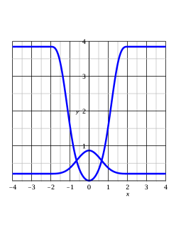
Figure 2. The graphics of W~(x)~𝑊𝑥\widetilde{W}(x) and w~(x)~𝑤𝑥\widetilde{w}(x), x(4,4)𝑥44x\in(-4,4)

Then: w~(x)>0~𝑤𝑥0\widetilde{w}(x)>0, for any x{0}𝑥0x\in{\mathbb{R}}\setminus\{0\} and min{w~(x):x}=w~(0)=0:~𝑤𝑥𝑥~𝑤00\min\{\widetilde{w}(x):x\in{\mathbb{R}}\}=\widetilde{w}(0)=0, see Figure 2.

In this case the method used in the proof of Theorem 2.1 produces interpolation.

See Example 4.2 in Section 4.

4. Some Examples. Case of Interpolation

Example 4.1.

Consider the following example of control points:

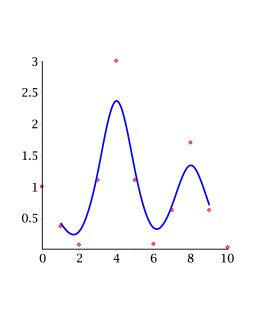
Ξ0={(xi,f(xi)):xi=i,f(x)=ex2+3e(x4)2+1.7e(x8)2,i=0,,10}.subscriptΞ0conditional-setsubscript𝑥𝑖𝑓subscript𝑥𝑖formulae-sequencesubscript𝑥𝑖𝑖formulae-sequence𝑓𝑥superscript𝑒superscript𝑥23superscript𝑒superscript𝑥421.7superscript𝑒superscript𝑥82𝑖010\Xi_{0}=\{(x_{i},f(x_{i})):x_{i}=i,\\ f(x)=e^{-x^{2}}+3e^{-(x-4)^{2}}+1.7e^{-(x-8)^{2}},\ i=0,\dots,10\}.

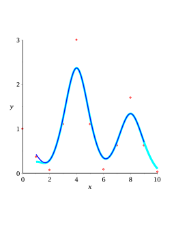
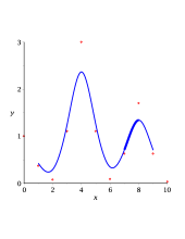
Here n=10𝑛10n=10, r=4𝑟4r=4, knots: ti=isubscript𝑡𝑖𝑖t_{i}=i, i=1,,14𝑖114i=1,\dots,14. The control points and cubic b-spline 𝜸(x)𝜸𝑥\boldsymbol{\gamma}(x) are illustrated on Figure 3. Here we used standart Maple expression BSplineCurve, see [9].
Refer to caption

Figure 3. The plots of data-set Ξ0subscriptΞ0\Xi_{0} and cubic b-spline in [1,9]19[1,9]

Using Remark 1 it is easy to construct the b-spline curve in whole interval [2,10]210[2,10] – see Figure 4.

Refer to caption

Figure 4. The plots of data-set Ξ0subscriptΞ0\Xi_{0} (red dots), cubic b-spline in [1,9]19[1,9] (blue curve) and moving least square approximation in [2,10]210[2,10] (cyan bold curve)

Let us apply Theorem 3.1 in the interval (5,6)56(5,6), for example. We have W(x)=B52,4(x+5+2)𝑊𝑥subscript𝐵524𝑥52W(x)=B_{5-2,4}(x+5+2) and moreover

W(x)>0,i=4,5,6,7;W(x)=0,i=0,1,2,3,8,9,10.formulae-sequence𝑊𝑥0formulae-sequence𝑖4567formulae-sequence𝑊𝑥0𝑖01238910W(x)>0,\ i=4,5,6,7;\quad W(x)=0,\ i=0,1,2,3,8,9,10.

Following the proof of theorem: let w(s)=1W(s)𝑤𝑠1𝑊𝑠w(s)=\dfrac{1}{W(s)}. Let x(5,6)𝑥56x\in(5,6) be a fixed point, then:

EtD1E=superscript𝐸𝑡superscript𝐷1𝐸absent\displaystyle E^{t}D^{-1}E= 12(1w(|x4|)+1w(|x5|)+1w(|x6|)+1w(|x7|))121𝑤𝑥41𝑤𝑥51𝑤𝑥61𝑤𝑥7\displaystyle\dfrac{1}{2}\left(\dfrac{1}{w(|x-4|)}+\dfrac{1}{w(|x-5|)}+\dfrac{1}{w(|x-6|)}+\dfrac{1}{w(|x-7|)}\right)
=\displaystyle= 12,12\displaystyle\dfrac{1}{2},

see (BS-3). Moreover

𝒂=D1E(EtD1E)1𝒄=D1E 2=(B2,4(x)B3,4(x)B4,4(x)B5,4(x)).𝒂superscript𝐷1𝐸superscriptsuperscript𝐸𝑡superscript𝐷1𝐸1𝒄superscript𝐷1𝐸2matrixsubscript𝐵24𝑥subscript𝐵34𝑥subscript𝐵44𝑥subscript𝐵54𝑥\displaystyle\boldsymbol{a}=D^{-1}E\left(E^{t}D^{-1}E\right)^{-1}\boldsymbol{c}=D^{-1}E\ 2=\begin{pmatrix}B_{2,4}(x)\\ B_{3,4}(x)\\ B_{4,4}(x)\\ B_{5,4}(x)\\ \end{pmatrix}.

So, we receive the classical b-spline formula in the interval (5,6)56(5,6):

γ2(x)=i=25W(xi)f(i)=i=25Bi,4(x)f(i).subscript𝛾2𝑥superscriptsubscript𝑖25𝑊𝑥𝑖𝑓𝑖superscriptsubscript𝑖25subscript𝐵𝑖4𝑥𝑓𝑖\gamma_{2}(x)=\sum\limits_{i=2}^{5}W(x-i)f(i)=\sum\limits_{i=2}^{5}B_{i,4}(x)f(i).

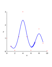
The b-splines in the intervals [5,6]56[5,6], [6,7]67[6,7], and [7,8]78[7,8] are ploted on Figure 5, respectively.
Refer to caption Refer to caption Refer to caption

Figure 5. The plots of b-spline in [5,6]56[5,6], [6,7]67[6,7], and [7,8]78[7,8], respectively (blue bold curve)
Example 4.2.

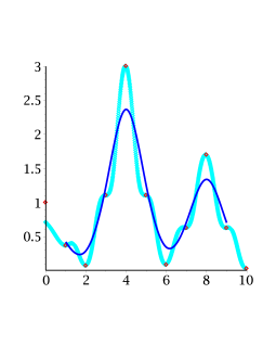
To construct the interpolation in the interval [x0,x10]subscript𝑥0subscript𝑥10[x_{0},x_{10}], following Remark 2, let us set δ=0.1𝛿0.1\delta=0.1, for example. Then

w~(x)=1W(x)+0.135,x.formulae-sequence~𝑤𝑥1𝑊𝑥0.135𝑥\widetilde{w}(x)=\dfrac{1}{W(x)+0.1}-\dfrac{3}{5},\quad x\in{\mathbb{R}}.

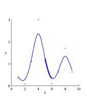
Applying the moving least-squares method (i.e. applying Remark 2 and Theorem 2.1 at each point x=l/100𝑥𝑙100x=l/100, l=1,,1000𝑙11000l=1,\dots,1000) we received the function presented in Figure 6.
Refer to caption

Figure 6. The plots of data (red dots), b-spline (blue), and interpolation (cyan, bold)

5. B-Spline Surfaces

Let {𝒑ij3:i,j=0,,n}conditional-setsubscript𝒑𝑖𝑗superscript3formulae-sequence𝑖𝑗0𝑛\{\boldsymbol{p}_{ij}\in{\mathbb{R}}^{3}:i,j=0,\dots,n\} be a set of (n+1)2superscript𝑛12(n+1)^{2} control points.

Let r𝑟r be an integer, 1rn+11𝑟𝑛11\leq r\leq n+1 (the order of spline).

We will use again the uniform knots, without multiplicity: ui=vi=isubscript𝑢𝑖subscript𝑣𝑖𝑖u_{i}=v_{i}=i, i=0,,n+r𝑖0𝑛𝑟i=0,\dots,n+r. Then, the corresponding b-spline surface of order r𝑟r is given by

𝒓(u,v)=i=0nj=0nBi,r(u)Bj,r(v)𝒑ij.𝒓𝑢𝑣superscriptsubscript𝑖0𝑛superscriptsubscript𝑗0𝑛subscript𝐵𝑖𝑟𝑢subscript𝐵𝑗𝑟𝑣subscript𝒑𝑖𝑗\boldsymbol{r}(u,v)=\sum\limits_{i=0}^{n}\sum\limits_{j=0}^{n}B_{i,r}(u)B_{j,r}(v)\boldsymbol{p}_{ij}.

Arguments similar to the proof of Theorem 3.1, yield to the following result.

Theorem 5.1.

Let:

  1. (1)

    d=2𝑑2d=2, n,r+𝑛𝑟subscriptn,r\in{\mathbb{Z}_{+}}, rn+1𝑟𝑛1r\leq n+1, f:[0,n+r]×[0,n+r]:𝑓0𝑛𝑟0𝑛𝑟f:[0,n+r]\times[0,n+r]\to\mathbb{R} be a continuous function.

  2. (2)

    𝒑ij=(i,j,f(i,j))subscript𝒑𝑖𝑗𝑖𝑗𝑓𝑖𝑗\boldsymbol{p}_{ij}=(i,j,f(i,j)), i=0,,n+r𝑖0𝑛𝑟i=0,\dots,n+r.

  3. (3)

    Let 𝜸(u,v)=(uvγ3(u,v))𝜸𝑢𝑣𝑢𝑣subscript𝛾3𝑢𝑣\boldsymbol{\gamma}(u,v)=\left(\begin{smallmatrix}u\\ v\\ \gamma_{3}(u,v)\end{smallmatrix}\right) be the b-spline of order r𝑟r and knots {(ui,vj)=(i,j):i,j=0,,n+r}conditional-setsubscript𝑢𝑖subscript𝑣𝑗𝑖𝑗formulae-sequence𝑖𝑗0𝑛𝑟\{(u_{i},v_{j})=(i,j):i,j=0,\dots,n+r\}.

Then there exists a weight function W(x,y)𝑊𝑥𝑦W(x,y), such that

γ3(x,y)=L^(f)(x,y),(x,y)[r1,n]×[r1,n].formulae-sequencesubscript𝛾3𝑥𝑦^𝐿𝑓𝑥𝑦𝑥𝑦𝑟1𝑛𝑟1𝑛\gamma_{3}(x,y)=\hat{L}(f)(x,y),\quad(x,y)\in[r-1,n]\times[r-1,n].
Example 5.1.

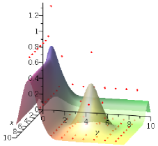
As an example, consider the following data
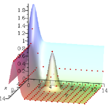
Ξ0={(xi,yj,f(xi)):xi=i,yj=j,f(xi,yj)=ex2+3e(y1)2+e(x6)2(y6)2,i=0,,10}.subscriptΞ0conditional-setsubscript𝑥𝑖subscript𝑦𝑗𝑓subscript𝑥𝑖formulae-sequencesubscript𝑥𝑖𝑖formulae-sequencesubscript𝑦𝑗𝑗formulae-sequence𝑓subscript𝑥𝑖subscript𝑦𝑗superscript𝑒superscript𝑥23superscript𝑒superscript𝑦12superscript𝑒superscript𝑥62superscript𝑦62𝑖010\Xi_{0}=\left\{(x_{i},y_{j},f(x_{i})):x_{i}=i,\ y_{j}=j,\right.\\ \left.f(x_{i},y_{j})=e^{-x^{2}}+3e^{-(y-1)^{2}}+e^{-(x-6)^{2}-(y-6)^{2}},\ i=0,\dots,10\right\}.

Refer to caption

Figure 7. Set of knots and plot of function f(x,y)𝑓𝑥𝑦f(x,y), x,y[0,14]𝑥𝑦014x,y\in[0,14]

Refer to caption

Figure 8. B-spline surface γ3(u,v)subscript𝛾3𝑢𝑣\gamma_{3}(u,v) in [1,9]×[1,9]1919[1,9]\times[1,9]

Refer to caption Refer to caption Refer to caption

Refer to caption Refer to caption Refer to caption

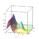
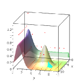
Figure 9. B-splines in [i,i+1]×[i,i+1]𝑖𝑖1𝑖𝑖1[i,i+1]\times[i,i+1], i=6,7,8𝑖678i=6,7,8 and corresponding zoomed segments

The set of control points 𝒑ij=(xiyjf(xi,yj)γ2(t))subscript𝒑𝑖𝑗subscript𝑥𝑖subscript𝑦𝑗𝑓subscript𝑥𝑖subscript𝑦𝑗subscript𝛾2𝑡\boldsymbol{p}_{ij}=\left(\begin{smallmatrix}x_{i}\\ y_{j}\\ f(x_{i},y_{j})\gamma_{2}(t)\end{smallmatrix}\right) and function f(x,y)𝑓𝑥𝑦f(x,y) are plotted in Figure 7.

Using the formula

L^(f)(x,y)=i=0nj=0n𝒑ijW(xi)W(xj).^𝐿𝑓𝑥𝑦superscriptsubscript𝑖0𝑛superscriptsubscript𝑗0𝑛subscript𝒑𝑖𝑗𝑊𝑥𝑖𝑊𝑥𝑗\hat{L}(f)(x,y)=\sum\limits_{i=0}^{n}\sum\limits_{j=0}^{n}\boldsymbol{p}_{ij}W(x-i)W(x-j).

we receive the plot of b-spline surface γ3(u,v)subscript𝛾3𝑢𝑣\gamma_{3}(u,v) in [1,9]×[1,9]1919[1,9]\times[1,9], see Figure 8.

If we need the plot of b-spline only in the segment [i0,i0+1]×[j0,j0+1]subscript𝑖0subscript𝑖01subscript𝑗0subscript𝑗01[i_{0},i_{0}+1]\times[j_{0},j_{0}+1], then

L^(f)(x,y)=i=i03i0j=j03j0𝒑ijW(xi)W(yj),^𝐿𝑓𝑥𝑦superscriptsubscript𝑖subscript𝑖03subscript𝑖0superscriptsubscript𝑗subscript𝑗03subscript𝑗0subscript𝒑𝑖𝑗𝑊𝑥𝑖𝑊𝑦𝑗\hat{L}(f)(x,y)=\sum\limits_{i=i_{0}-3}^{i_{0}}\sum\limits_{j=j_{0}-3}^{j_{0}}\boldsymbol{p}_{ij}W(x-i)W(y-j),

see Figure 9.

References

  • [1] Gary D. Knott, Interpolating Cubic Splines, Springer Science & Business Media (2000), 244 pages.
  • [2] N.M. Patrikalakis, T. Maekawa, W. Cho, http://web.mit.edu/hyperbook/Patrikalakis-Maekawa-Cho/
  • [3] E.T.Y. Lee, A simplified b-spline computation routine, Computing, Springer-Verlag, 29, No. 4 (1982), 365–371, doi: 10.1007/BF02246763.
  • [4] E.T.Y. Lee, Comments on some b-spline algorithms, Computing, Springer-Verlag, 36, No. 3 (1986), 229–238, doi: 10.1007/BF02240069.
  • [5] Marc Alexa, Johannes Behr, Daniel Cohen-Or, Shachar Fleishman, David Levin, Claudio T. Silva, Point-Set Surfaces, http://www.math.tau.ac.il/ levin/
  • [6] D. Levin, The approximation power of mooving least-squares, http://www.math.tau.ac.il/ levin/
  • [7] D. Levin, Mesh-independent surface interpolation, http://www.math.tau.ac.il/ levin/
  • [8] D. Levin, Stable integration rules with scattered integration points, Journal of Computational and Applied Mathematics, 112 (1999), 181-187, http://www.math.tau.ac.il/ levin/
  • [9] Maple 2015 Hepl System, http://www.maplesoft.com/
  • [10] Dicho Stratiev, Ivaylo Marinov, Rosen Dinkov, Ivelina Shishkova, Ilian Velkov, Ilshat Sharafutdinov, Svetoslav Nenov, Tsvetelin Tsvetkov, Sotir Sotirov, Magdalena Mitkova, Nikolay Rudnev, Opportunity to improve diesel-fuel cetane-number prediction from easily available physical properties and application of the least-squares method and artificial neural networks, Energy & Fuels, 29, No. 3 (2015).
  • [11] Arne Laksøa, Børre Bang, Lubomir T. Dechevsky, Geometric modelling with beta-function b-splines, I: Parametric curves, International Journal of Pure and Applied Mathematics, 65, No. 3 (2010), 339-360.
  • [12] Arne Laksøa, Børre Bang, Lubomir T. Dechevsky, Geometric modelling with beta-function b-splines, II: Tensor-product parametric surfaces, International Journal of Pure and Applied Mathematics, 65, No. 3 (2010), 361-380.