Extended X-ray Monitoring of Gravitational Lenses with Chandra and Joint Constraints on X-ray Emission Regions

Abstract

We present an X-ray photometric analysis of six gravitationally lensed quasars, with observation campaigns spanning from $5$ to $14$ years, measuring the total ($0.83-21.8$ keV restframe), soft ($0.83-3.6$ keV), and hard ($3.6-21.8$ keV) band image flux ratios for each epoch. Using the ratios of the model-predicted macro-magnifications as baselines, we build differential microlensing light curves and obtain joint likelihood functions for the average X-ray emission region sizes. Our analysis yields a Probability Distribution Function for the average half-light radius of the X-Ray emission region in the sample that peaks slightly above $1$ gravitational radius and with nearly indistinguishable $68\%$ confidence (one-sided) upper limits of $17.8$ and $18.9$ gravitational radii for the soft and hard X-ray emitting regions, assuming a mean stellar mass of $0.3$ $M_{\odot}$. We see hints of energy dependent microlensing between the soft and hard bands in two of the objects. In a separate analysis on the root-mean-square (RMS) of the microlensing variability, we find significant differences between the soft and hard bands but the sign of the difference is not consistent across the sample. This suggests the existence of some kind of spatial structure to the X-ray emission in an otherwise extremely compact source. We also discover a correlation between the RMS microlensing variability and the average microlensing amplitude.

1 Introduction

X-ray emission is one of the defining characteristics of active galactic nuclei (AGN). However, most properties of the X-ray corona are obtained only through spectral analyses, since neither current nor near-future instrumentation can resolve the X-ray emitting regions of AGN. Reverberation mapping and quasar microlensing provide the only probes of the spatial structure of the different AGN components, with the latter better suited to the more compact regions like the X-ray corona or the accretion disk. Reverberation mapping studies have succeeded in mapping the more spatially extended regions such as the broad line regions (e.g., Bentz et al., 2009; Zu et al., 2011; Bentz et al., 2013; Kollatschny et al., 2014), the dust torus (e.g., Koshida et al., 2014), and with limited results for accretion disks (e.g., Shappee et al., 2014; Fausnaugh et al., 2016).

Microlensing refers to the micro-arcsecond effects produced by light ray deflections of emision from a background source by foreground stars. It has the advantage over reverberation mapping in that the signal only becomes stronger as the source becomes more compact. The Einstein radius gives a typical scale of

$$R_{E}=D_{ol}\sqrt{\frac{4GM}{c^{2}}\frac{D_{ls}}{D_{ol}D_{os}}},$$ (1)

where $M$ denotes the deflector mass and $D_{ol}$, $D_{os}$, and $D_{ls}$ are the angular diameter distances between the observer, lens, and source respectively. If the apparent size of the source is comparable or smaller in size than the Einstein radius, typically a few light-days, the observed flux varies because the magnification changes as the source, lens, and observer move relative to each other (see, e.g., the review by Wambsganss, 2006). This makes extragalactic microlensing a unique tool for probing the spatial structure of the central region of quasars, because most AGN components are comparable in size to the Einstein radius or smaller. As a result, microlensing has been successfuly used to obtain size estimates for the broad line region spanning several tens of light days (e.g., Sluse et al., 2012; Guerras et al., 2013a), the accretion disk spanning $\sim$10 light-days (e.g., Morgan et al., 2008; Mediavilla et al., 2011a; Jiménez-Vicente et al., 2014), and the X-ray corona of $\sim$1 light-day (e.g., Dai et al., 2010; Pooley et al., 2012; Morgan et al., 2012; Mosquera et al., 2013; Blackburne et al., 2014, 2015; MacLeod et al., 2015).

Here, we present updated X-ray light curves for a sample of $6$ lensed quasars with redshifts between $z_{s}=1.3$ and $z_{s}=2.3$. We derive total, soft, and hard energy band light curves in Section 2 and examine them for evidence of microlensing. We perform a simple analysis of several aspects of the microlensing variability in Section 3. In Section 4 we derive a Probability Distribution Function (PDF) for the average size of the X-ray emitting region in the sample. Section 5 presents a summary of the results. We assume a flat $\Lambda$CDM cosmology with $H_{0}=70~{}{\rm km~{}s^{-1}Mpc}^{-1}$, $\Omega_{m}=0.3$, and $\Omega_{\Lambda}=0.7$.

2 Image Models and Photometry

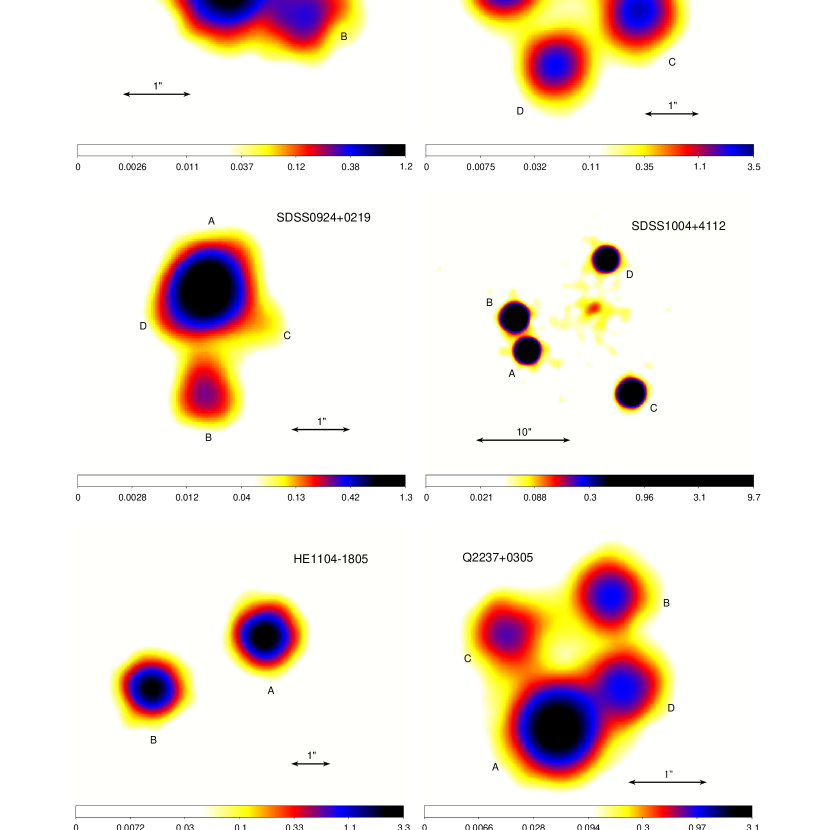
We observed five gravitationally lensed quasars with Chandra/ACIS (Weisskopf et al., 2002; Garmire et al., 2003) in Cycles 14–16 for a total exposure time of 810 ks. For each object, we obtained 6–8 sparse monitoring observations over a period of 2–3 years. We also include any archival data for the five systems and an aditional one in our analysis, adding up to six gravitational lenses. All data (both new and archival) were re-calibrated and processed with the latest CIAO 4.7 software. Figure 1 presents stacked images of the six systems, and Table 1 summarizes their basic properties. Only in SDSS 1004+4112 are the lensed images easily resolved by Chandra so that we could do a simple aperture photometry. For this system, we also correct for the background emission from the lensing cluster using arc-shaped regions opposed to each image with respect to the center of the X-ray cluster. For the rest of the systems, we used PSF fitting based on the known relative positions of the images as they are listed in the CASTLES website (see references therein) to model the image fluxes, because the typical angular image separation is not much bigger than the $\sim 0\arcsec.5$ arcsec on-axis PSF of Chandra and aperture photometry would be contaminated by the flux from nearby images. The details of our approach to PSF fitting and photometry can be found in Chen et al. (2012) who analysed data from our previous observational campaigns.

Unlike Chen et al. (2012), we used a fixed rest frame energy boundary of $3.6$ keV to define the rest frame soft ($0.8-3.6$ keV) and hard ($3.6-21.8$ keV) bands. This both produces comparable count rates for each band and leads to a well-defined combined analysis in Section 4. Count rates are background subtracted and corrected for both Galactic absorption and absorption by the lens galaxy. To estimate the latter, we closely followed the steps detailed by Chen et al. (2012). We fit a simple power law with a Gaussian emission line model to the stacked spectra of individual images. The absorption of the lens galaxy was allowed to vary independently in the fit for each image, while the power law index was assumed to be the same for all the images of each quasar. Further details of the absorption correction in our data will be presented in a companion paper (Steele et al. 2017, in preparation) which focuses on the spectral analysis of the sample. Tables 3 to 8 present the absorption-corrected count rates for each lens.

We also set limits on the flux of any central image found by combining all epochs. This is not feasible for SDSS1004+4112, which is known to have a central image (see Inada et al., 2008), because this is also where the cluster X-ray emission peaks (see Ota et al., 2006). Relative to the mean flux of the faintest observed image, the upper limits on the relative flux of any central image are $0.64,0.009,1.0,0.036,0.019$ for QJ 0158$-$4325, HE 0435$-$1223, SDSS 0924+0219, HE 1104$-$1805, and Q 2237+0305, respectively, at 68% confidence level. Based on the expected flux ratios of central images (see Keeton et al., 2003), only the limit for HE 0435$-$1223 is strong enough to be useful as an upper limit on the central surface mass density of the lens model.

3 Microlensing Analysis

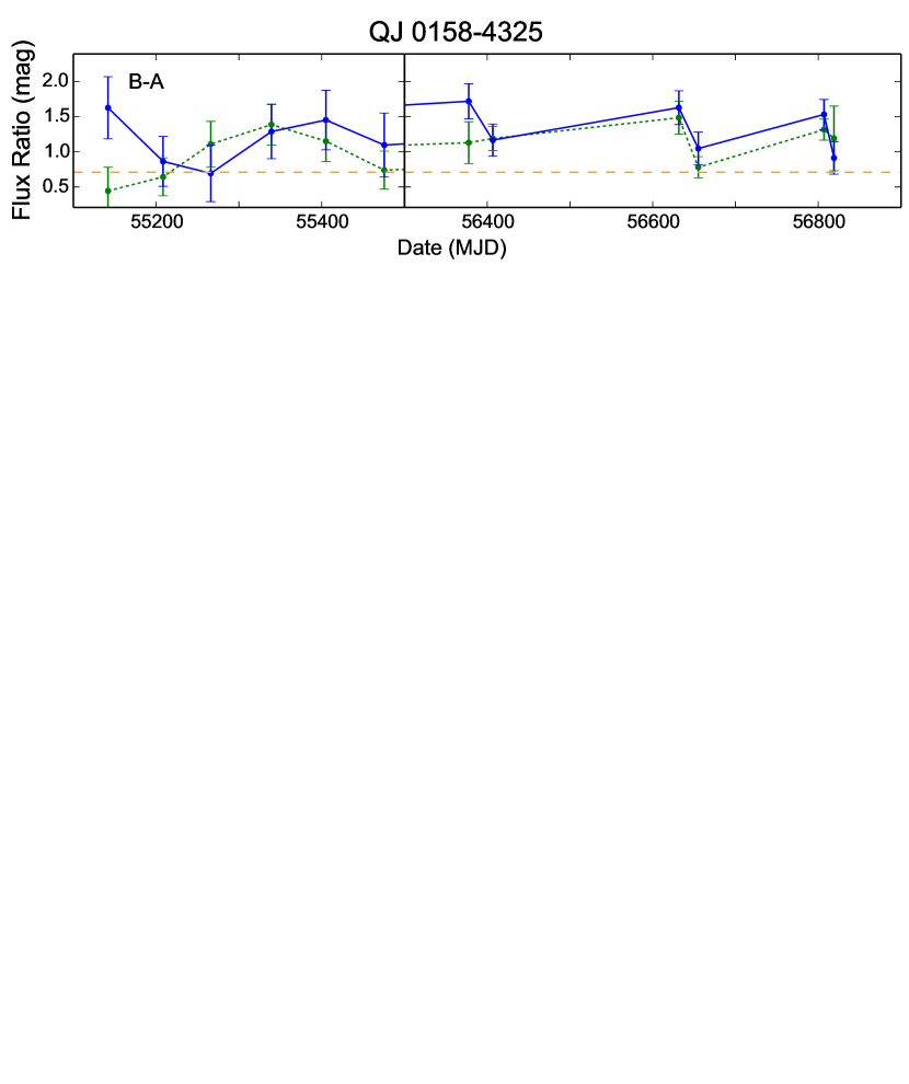
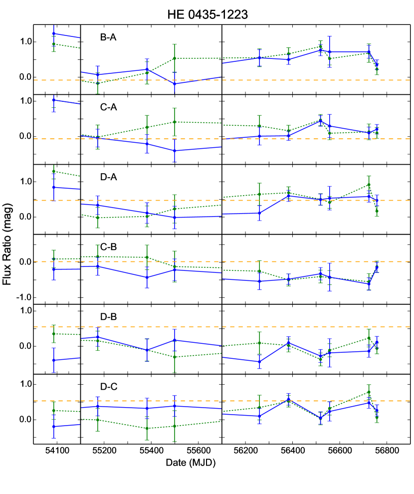
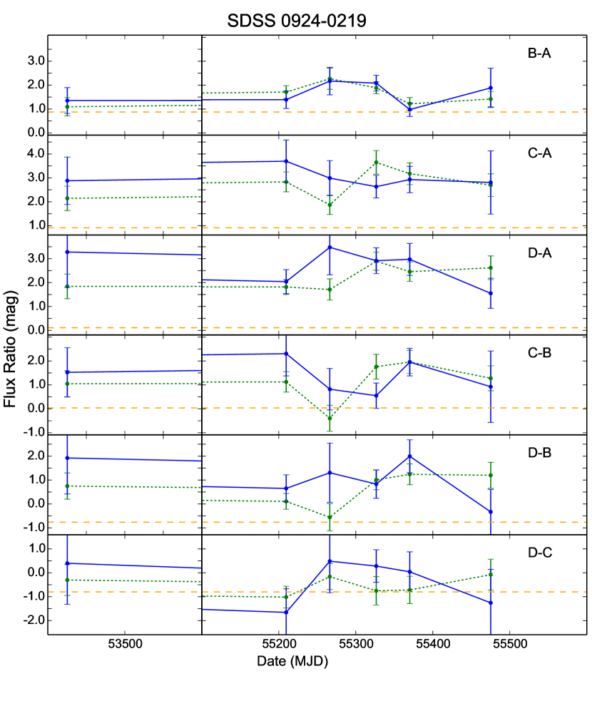
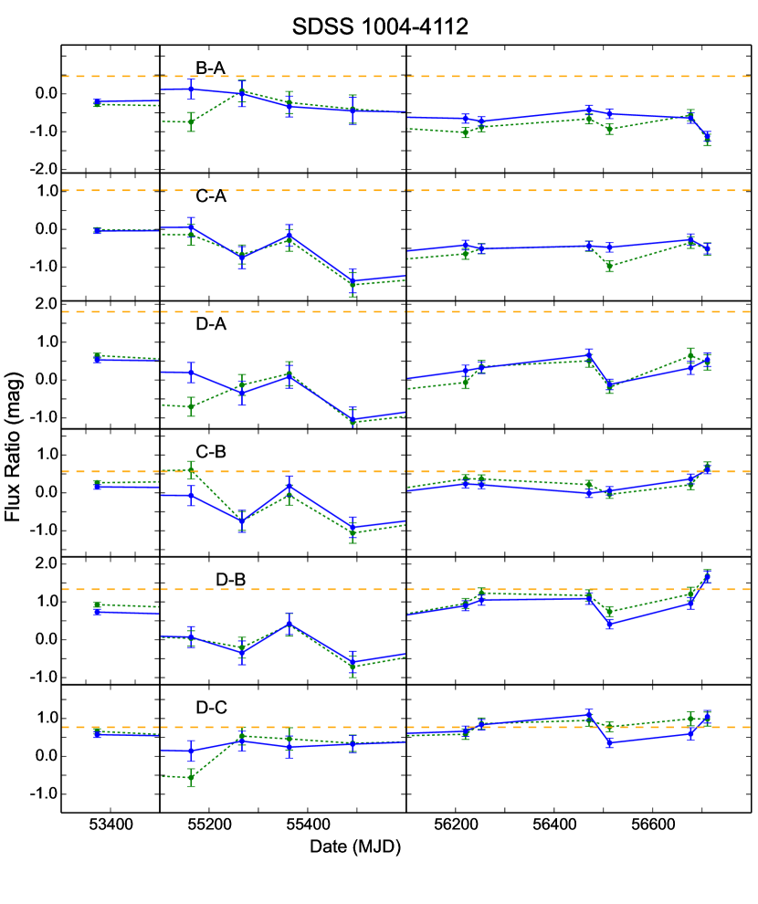
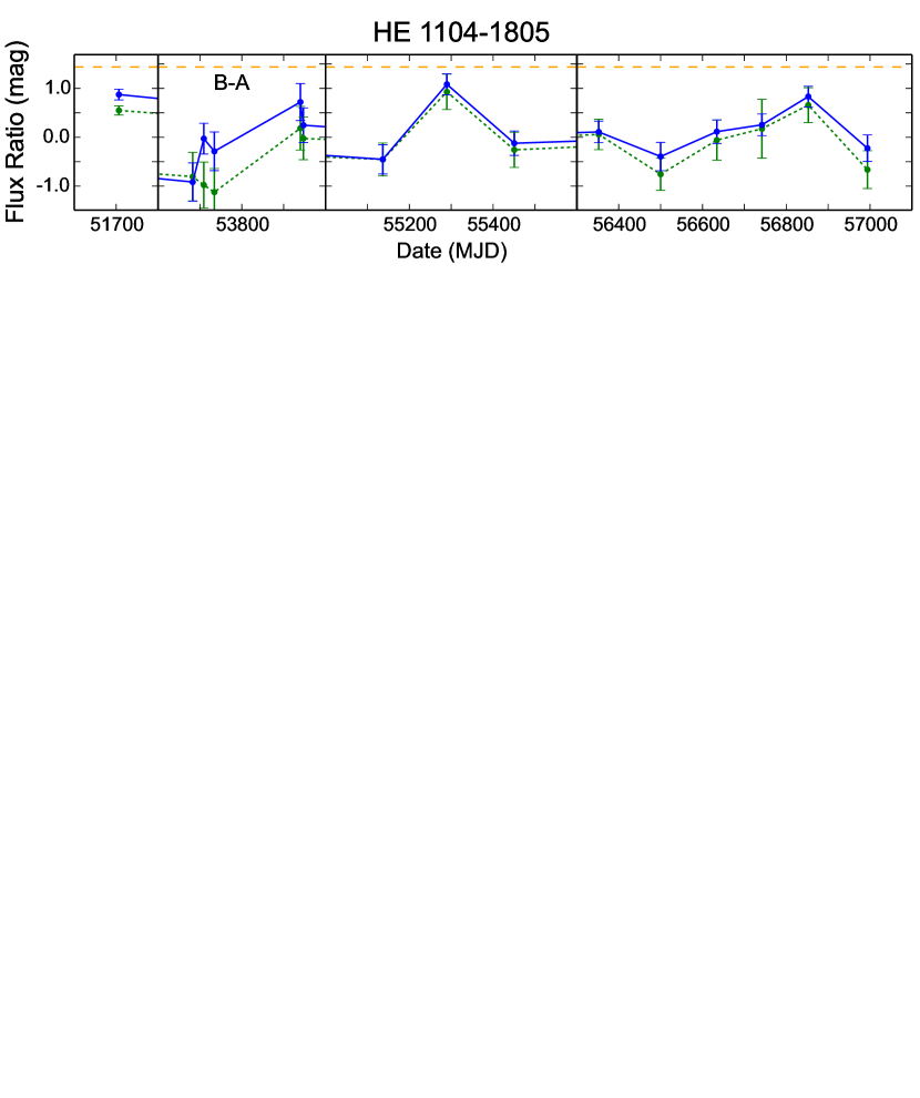
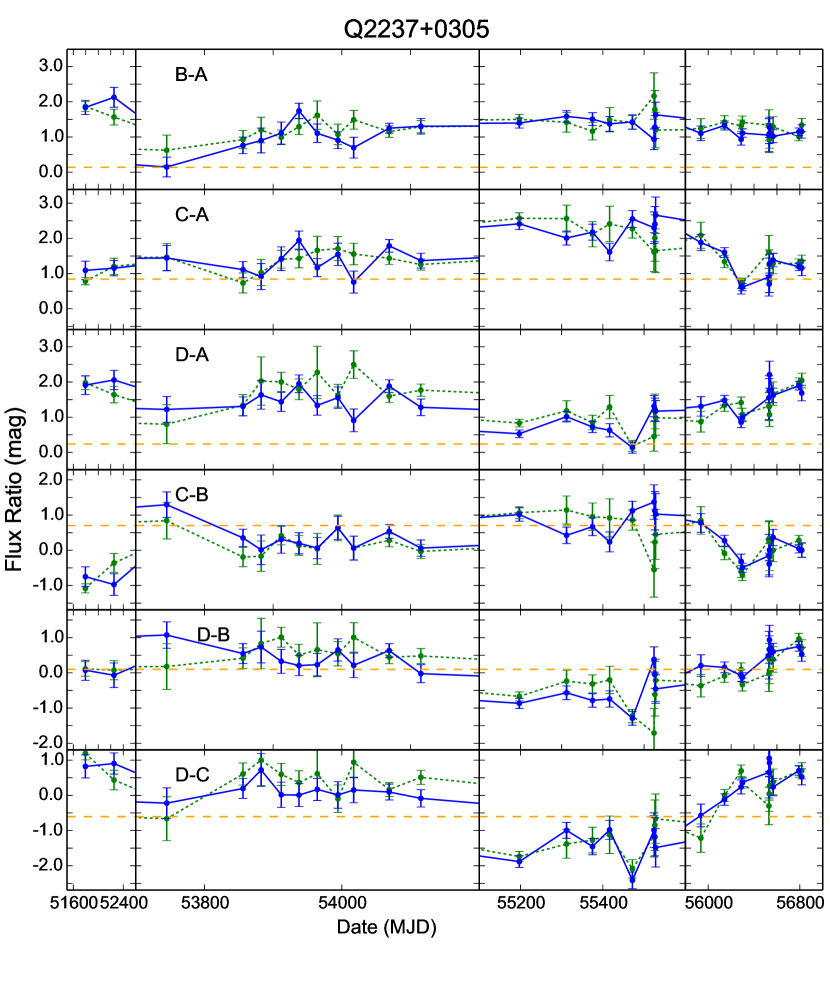
We want to compare the microlensed flux ratios between images with the intrinsic flux ratios that are not affected by microlensing (baseline ratios). After correction for any absorption, the baseline flux ratios are primarily determined by the smooth potential of the lens galaxy, although they may be perturbed by substructures in the lens galaxy such as satellite halos (Kochanek & Dalal, 2004; Zackrisson & Riehm, 2010). Ideally, the baseline ratios are measured at wavelengths where the quasar emitting region is much larger than the Einstein radius (several light days for lensed quasars) and therefore not sensitive to microlensing. This is generally true of radio, rest-frame mid-IR and narrow line emission. When that is not possible, baseline ratios can be approximated using the macro magnifications from lens models. We adopt the latter approach, with baseline ratios derived from macro lens models. The values adopted are shown as horizontal lines in Figures 2–7.

The measured flux $f_{ij}$ (count rate) of the i-th image at the j-th epoch

$$f_{ij}=s_{j}\cdot\mu_{i}\cdot\xi_{ij},$$ (2)

is the source flux $s_{j}$ magnified by a combination of macro-lens and microlensing magnifications $\mu_{j}$ and $\xi_{ij}$, respectively. The flux ratio between two images $A$ and $B$ is

$$\frac{f_{Bj}}{f_{Aj}}=\frac{s_{Bj}}{s_{Aj}}\cdot\frac{\mu_{B}}{\mu_{A}}\cdot\frac{\xi_{Bj}}{\xi_{Aj}}.$$ (3)

We are interested in $\xi_{Bj}/\xi_{Aj}$, but we measure the fluxes ${f_{Bj}}$ and ${f_{Aj}}$. An additional complication is that the source flux ratio is really

$$\frac{s_{Bj}}{s_{Aj}}=\frac{s(t)}{s(t+\delta t_{AB})},$$ (4)

which includes a propagation time delay $\delta t_{AB}$ (Refsdal, 1964; Cooke & Kantowski, 1975) that cannot be easily removed from the sparsely sampled X-ray light curves as is done in optical studies (e.g., Kochanek et al., 2014; Tewes et al., 2013). If $\delta t_{AB}$ is much smaller than the typical time scale of intrinsic variability, the effects of the time delay become unimportant. This is certainly the case of Q 2237+0305 where the time delays are constrained to be $<1$ day (Dai et al., 2003). The other extreme in our sample is SDSS 1004+4112, where the delays are as long as several years (Fohlmeister et al., 2008). In these cases, the time delays combined with intrinsic source variability add “noise” to the light curves that can be interpreted as additional microlensing variability. We will follow the usual procedure (e.g., Schechter et al., 2014) and assume that $s_{Bj}/s_{Aj}\approx 1$. This strategy is safest for image pairs with shorter lens delays. Using this assumption, Equation 3 becomes

$$\chi_{BA}(t_{j})=\frac{\xi_{Bj}}{\xi_{Aj}}=\left[\frac{f_{Bj}}{f_{Aj}}\right]\cdot\left[\frac{\mu_{B}}{\mu_{A}}\right]^{-1}.$$ (5)

This microlensing amplitude should not be confused with simple flux ratios which include no corrections for the macro lens magnifications. The microlensing magnification ratio can also be expressed in magnitudes to facilitate comparison with optical microlensing studies where the image fluxes and macro magnification ratios are now expressed in magnitudes,

$$m_{B}-m_{A}=-2.5\log(f_{B}/f_{A})$$ (6)

$$m_{B}^{0}-m_{A}^{0}=-2.5\log(\mu_{B}/\mu_{A})$$ (7)

$$\Delta m_{AB}=(m_{B}-m_{A})-(m_{B}^{0}-m_{A}^{0}).$$ (8)

Table 9 summarizes the values we adopt for the macro magnifications, where the total magnification $\mu_{i}$ is derived from the estimated convergence $\kappa_{i}$ and shear $\gamma_{i}$ at each image position according to $\mu_{i}=[(1-\kappa_{i})^{2}-\gamma_{i}^{2}]^{-1}$ (see, e.g., Narayan & Bartelmann, 1996). These estimates of $\kappa_{i}$ and $\gamma$ are obtained by fitting a model for the overall potential of the lens galaxy to the lens data. We fit a singular isothermal ellipsoid with external shear (SIE+g) to both QJ 0158$-$4325 and HE 1104$-$1805 using Lensmodel (Keeton, 2001). For SDSS 1004+4112, we used the cluster mass model for this lens by Oguri (2010), ($\kappa,\gamma$ values given in private communication). For the rest of the objects, we used SIE+g results from the literature as listed in Table 9.

We also need the surface density of stars $\kappa_{*}$ relative to the total surface density $\kappa$. We combined the astrometry of each lens with the compilation of lens galaxy effective radii in Oguri et al. (2014) to estimate the ratio $R/R_{eff}$ between the radial distance of each image from the lens center and the effective radius of the lens. We then used the best fit model for $\kappa_{*}/\kappa$ from Oguri et al. (2014) to estimate the stellar surface density, except in the case of SDSS 1004+4112. The lens SDSS 1004+4112 is a special case because it is a cluster lens, where the member galaxies are further from the images than in single-galaxy lenses. We adopted an arbitrarily low value $\kappa_{*}/\kappa=0.03$ as pleausible estimate of the low optical depth associted with intracluster stars. Q 2237+0305 is also a special case because the images are seen through a galactic bulge, and here $\kappa_{*}/\kappa\simeq 0.8$ because the images are seen through a galactic bulge. The average value of $\kappa_{*}/\kappa$ is in reasonable agreement with previous estimates (Jiménez-Vicente et al., 2015). The results are presented in Table 9.

There are two ways in which microlensing effects may manifest themselves. One is through the time variability in the flux ratios, which is independent of the baseline flux ratios but can be affected by intrinsic variability modulated by time delays. The second is if the X-Ray flux ratios differ from the estimated base line ratios. The difference allows a quantitative measurement of microlensing but it is only reliable to the extent that the baseline flux ratios are accurate. We summarize the differential microlensing in Figures 2–7, where the flux ratios for the hard and soft X-ray bands are compared and the baseline ratios are shown as horizontal lines. The distance between the data points and the horizontal lines represent the differential microlensing. The figures show a complex pattern of time variability attributable to microlensing and, to so some extent, to noise introduced by time variabiliy.

3.1 An Independent Test for Energy-Dependent Microlensing

The X-ray emission regions of lensed quasars appear to be more compact than the disk emission seen at ultraviolet or optical wavelengths because the X-ray microlensing amplitude is consistently higher (e.g., Morgan et al., 2008; Chartas et al., 2009; Dai et al., 2010; Pooley et al., 2012; Mosquera et al., 2013; Schechter et al., 2014). This has been successfully used to map the size of the accretion disk at different wavelengths (Poindexter et al., 2008; Mediavilla et al., 2011a; Blackburne et al., 2011), but X-ray microlensing analyses to date have found that the hard and soft band X-ray emission regions are of similar size (Morgan et al., 2012; Mosquera et al., 2013; Blackburne et al., 2014, 2015). Here we want to test if the new data remain consistent with the null hypothesis that the microlensing amplitude is the same for both bands. In the absence of any band-dependent difference in the microlensing amplitude, the data should be consistent with the soft and hard bands having a common microlensing magnification ratio $\xi_{ij}$ (see Equation 5). We can test for this by optimising the statistic

$$\chi^{2}=\sum_{i,j}{\left[\frac{\left(f^{\rm hard}_{ij}-(s^{\rm hard}_{j}\cdot\mu_{i}\cdot\xi_{ij})\right)^{2}}{\left(\sigma^{\rm hard}_{ij}\right)^{2}}+\frac{\left(f^{\rm soft}_{ij}-(s^{\rm soft}_{j}\cdot\mu_{i}\cdot\xi_{ij})\right)^{2}}{\left(\sigma^{\rm soft}_{ij}\right)^{2}}\right]},$$ (9)

with respect to the source fluxes ($s^{\rm soft}_{j}$, and $s^{\rm hard}_{j}$) and the microlensing magnification ratio $\xi_{ij}$. If the source sizes are comparable, we should obtain a good fit using a single value for the microlensing magnification. The macrolens magnifications $\mu_{i}$ are fixed to the estimates from Table 9 and should be the same for all energy bands. The subscripts $i$ and $j$ refer to image and epoch respectively.

We can apply this test to the $4$ image lenses, finding reduced $\chi^{2}$ values of $0.79,0.94,1.5,$ and $1.4$ for HE 0435$-$1223, SDSS 0924+0219, SDSS 1004+4112, and Q 2237+0305 respectively, given $23,15,25,$ and $63$ degrees of freedom. The p-values are $0.75,0.52,0.05,$ and $0.01$. This implies the existence of energy dependent microlensing in Q 2237+0305 and, to a lesser extent, in SDSS 1004+4112. It must be noted that a high $\chi^{2}$ value can be the result of consistently wider amplitudes of either the hard or soft microlensing ratios. However, it may also happen as a result of non related signals of similar amplitude. Therefore a connection between this results and an intuitive interpretation of Figures 2–7 is not straightforward.

3.2 Root-Mean-Square of Microlensing Variability

Microlensing flux variations occur as the stars in the lens galaxies move relative to the background source, producing a complex variability pattern. Here we want to explore the root-mean-square (RMS) of the microlensing amplitude as an observable that can potentially be related numerically to the physical properties of the lens system. This is a reasonable assumption since a small source crossing a region with high density of caustics will show larger flux variations. If $\chi_{BA}(t_{i})$ is the microlensing amplitude (as defined in Equation 5) of a certain image pair at epoch $t_{i}$, then we define

$$\overline{\chi}_{BA}=\frac{1}{N}\sum_{i=1}^{N}\chi_{BA}(t_{i})$$ (10)

$$\chi_{BA}^{[RMS]}=\sqrt{{\frac{1}{N-1}}\sum_{i=1}^{N}(\chi_{BA}(t_{i})-\overline{\chi}_{BA})^{2}}$$ (11)

Table 2 lists the these two statistics for the full, soft, and hard bands along with their uncertainties. To quantify the significance of the differences between the soft and hard band RMS values, Table 2 also shows the p-values for rejecting the null hypothesis of identical distributions computed with a Welch two-tail test. The p-values suggest a distinct physical origin for the soft and hard band at a significance greater than $2\sigma$ confidence level in $8$ out of $20$ image pairs, and in $12$ out of $20$ pairs at a significance level greater than $1\sigma$. However, the sign of the difference between the hard and the soft band RMS is not consistent accross the sample, i.e. this difference does not always show the same sign across the three components of each quadruple quasar. This suggests the need to compare the results with an analysis of their a priori probabilities (Guerras et al. 2017, in preparation).

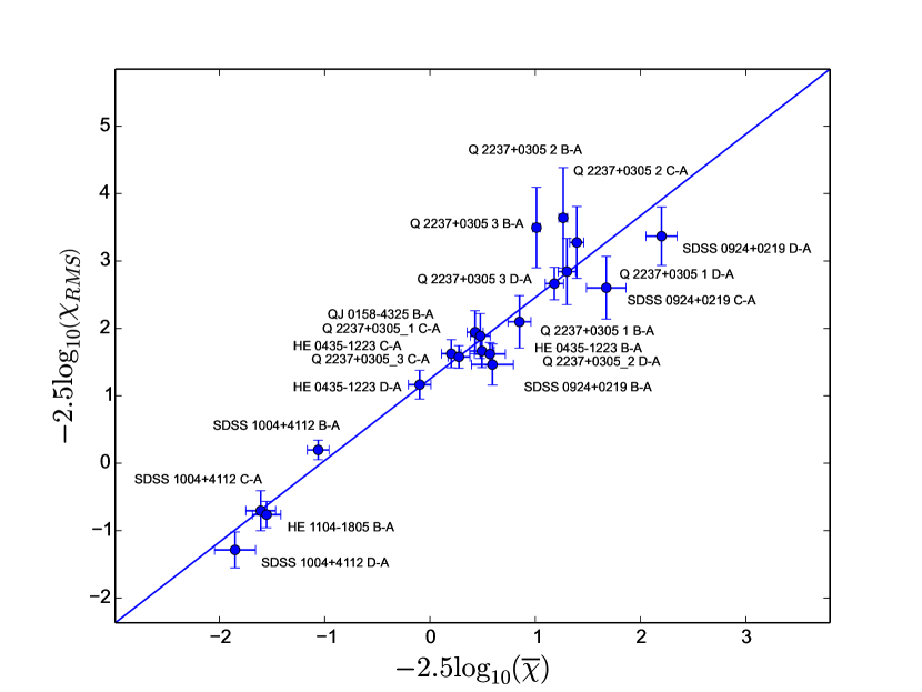
Figure 8 shows that the RMS $\chi^{[RMS]}$ and mean $\overline{\chi}$ microlensing signal are correlated. We find a Pearson correlation coefficient of $R=0.96^{+0.03}_{-0.06}$ ($95\%$ CL) and a best fit correlation of

$$\log_{10}\left(\chi^{[RMS]}\right)=(1.21\pm 0.08)\cdot\log_{10}\big{(}\overline{\chi}\big{)}-(0.50\pm 0.03).$$ (12)

This relationship suggests that the RMS may be a useful observable to better constrain the physical properties of lensed quasars. We will explore these issues further in Guerras et al. (2017, in preparation).

4 Source Size Estimates

Next we are interested in analysing the departures of the flux ratios from the base line ratios to determine the source size. The first step is a quantitative characterisation of such departures. When the observation campaigns cover short periods as compared with the microlensing variability timescales, a common approach is to assume that the span of the data is too short to observe microlensing variability. Several epochs are then averaged (e.g., Pooley et al., 2012; Jiménez-Vicente et al., 2015; Muñoz et al., 2016) and the resulting averages are compared with the numerical predictions for one single epoch per image pair (e.g., Mediavilla et al., 2009; Blackburne et al., 2011; Guerras et al., 2013a).

There are two characteristic microlensing variability timescales. One is the Einstein radius (Equation 1) crossing time, which is generally quite long, and a second, shorter timescale associated with the source crossing time. Table 1 summarizes estimates for both timescales from Mosquera & Kochanek (2011). These estimates strongly suggest that the comparison of simple averages of the light curves against single-epoch model predictions will be suboptimal here because our present data have time spans long enough that we should expect microlensing variability. By collapsing the light curves into average values, we could lose information because the behaviour of the average signal may not be well-modelled by single-epoch predictions.

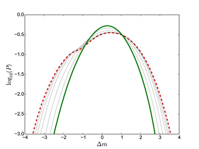
To explore the impact of averaging long observation campaigns on the probability of differential microlensing magnification, we can compare computer-generated probability distributions (details on their generation are given in Section 4.1) of single-epoch differential microlensing with analogous simulations where the predicted quantity is the average of differential microlensing along randomly orientated tracks whose length in Einstein Radii and number of observations match those in our data sample based on the scales in Table 1. Figure 9 illustrates this for Q 2237+0305 (C-A). Based on the $13.6$ year timespan of our data, and the estimate given by Mosquera & Kochanek (2011) of the time it takes the source to cross the Einstein radius in this system, the source has moved roughly $1.7$ $R_{E}$. We computed the mean microlensing signal observed by averaging over 30 evenly spaced epochs where the source moves from $0$ $R_{e}$ (i.e. a single epoch) up to $1.7$ $R_{E}$. The distribution of mean magnifications begins to narrow relatively quickly, particularly in the wings of the distributions. Thus, not taking into account the time averaging will lead to the derivation of an overly large source size because the source size must compensate for the neglected temporal smoothing. One compromise to address this problem is to only average epochs separated by shorter timescales (as done by e.g., Muñoz et al., 2016). We will instead use numerical models that take the length of each observation campaign into account.

We will derive a probability distribution for the half-light radius of the source, using all 4 or 2 images simultaneously. Given one object, the flux (count rate) of image $\alpha$ expressed in magnitudes at epoch $t_{i}$ is

$$m^{obs}_{\alpha}(t_{i})=m_{0}(t_{i})+\mu_{\alpha}+\xi_{\alpha}(t_{i})$$ (13)

where $m_{0}(t_{i})$ is the intrinsic magnitude of the source at epoch $t_{i}$, $\mu_{\alpha}$ is the macrolens magnification of image $\alpha$ and $\xi_{\alpha}(t_{i})$ is the microlensing magnification of image $\alpha$ at epoch $t_{i}$. Following Kochanek (2004) we first eliminate the intrinsic magnitude of the source by optimising a source model $m_{0}(t_{i})$ simultaneously to fit all the images:

$$\chi^{2}(t_{i})=\sum_{\alpha}\Big{(}\frac{m^{obs}_{\alpha}(t_{i})-[m_{0}(t_{i})+\mu_{\alpha}+\xi_{\alpha}(t_{i})]}{\sigma_{\alpha}}\Big{)}^{2}$$ (14)

After substituting the best source model $m_{0}(t_{i})$ the statistic in Eq. 14 reduces to

$$\chi^{2}(t_{i})=\sum_{\alpha}\sum_{\beta<\alpha}\Big{(}\frac{\left(m^{obs}_{\alpha}(t_{i})-[\mu_{\alpha}+\xi_{\alpha}(t_{i})]\right)-\left(m^{obs}_{\beta}(t_{i})-[\mu_{\beta}+\xi_{\beta}(t_{i})]\right)}{\sigma_{\alpha\beta}}\Big{)}^{2}$$ (15)

where the errors $\sigma_{\alpha\beta}$ are computed according to Equation $(7)$ in Kochanek (2004). This expression can be rearranged as

$$\chi^{2}(t_{i})=\sum_{\alpha}\sum_{\beta<\alpha}\Big{(}\frac{\Delta m^{obs}_{\beta\alpha}-\Delta m_{\beta\alpha}}{\sigma_{\beta\alpha}}\Big{)}^{2}$$ (16)

where $\Delta m^{obs}_{\beta\alpha}=\left(m^{obs}_{\beta}(t_{i})-\mu_{\beta}\right)-\left(m^{obs}_{\alpha}(t_{i})-\mu_{\alpha}\right)$ is the observed microlensing magnification as defined in Equation 8 and $\Delta m_{\beta\alpha}=\xi_{\beta}(t_{i})-\xi_{\alpha}(t_{i})$ is the microlensing magnification predicted by a numerical model. We explain the generation of the $\Delta m_{\beta\alpha}$ in Section 4.1.

Given the results for one trial, the likelihood of the source size for each epoch $i$ can be obtained by adding the likelihoods of a high number $N$ of trials,

$$L_{i}(r_{s})\propto\sum^{N}\exp{\Big{(}-\frac{1}{2}\chi_{i}^{2}\Big{)}}.$$ (17)

Following other studies, e.g. Muñoz et al. (2016), Jiménez-Vicente et al. (2015), we will collapse the light curves by averaging them to single time independent values $m^{obs}_{\alpha}$. The difference here will be in the model we use to generate the predicted distribution of the differential microlensing amplitudes $p\big{(}\Delta m_{\beta\alpha}\big{|}r_{s}\big{)}$. Rather than simply using the results for a single point, we will use averages obtained from random sets of data tracks that emulate the length and time sequence of the measurements available for each lens. Once we get a time-independent likelihood function $L(r_{s})$ for each lensed quasar, the joint probability density function is obtained as the normalised product of the individual likelihood functions,

$$P(r_{s})\propto\prod_{j}L_{j}(r_{s}).$$ (18)

4.1 Computer-generated probability distributions

To obtain the probability distributions $p\big{(}\Delta m_{\beta\alpha}\big{|}r_{s}\big{)}$ for each image pair and source size, we generated magnification patterns based on the $3$ local parameters for each image given in Table 9 (the local surface mass density $\kappa$, the shear $\gamma$, and the fraction of the local surface density in stars $\kappa_{*}/\kappa$). The stars are assigned a fixed mass of $M_{*}=0.3M_{\odot}$, since it has been shown that microlensing statistics depend little on the stellar mass function (e.g., Wambsganss, 1992; Mediavilla et al., 2015). The size estimates can be easily re-scaled to a different mean mass as $r_{s}\propto\sqrt{M_{*}}$.

To model the effect of the finite source size, we convolve the maps with a Gaussian kernel $I(r)\propto\exp[-r^{2}/(2r_{s}^{2})]$. For comparisons to other profiles, the half-light radius $r_{1/2}=1.18$ $r_{s}$ should be used since estimates of $r_{1/2}$ are insensitive to profile changes (Mortonson et al., 2005). The size of the X-ray corona is expected to be proportional to the mass of the central black hole (Mosquera et al., 2013; Jiménez-Vicente et al., 2015), so a natural choice for the source scaling is in units of gravitational radii $R_{g}=GM_{BH}/c^{2}$ based on the estimates given in Table 1. For this case we used a grid where $R_{s}/R_{g}=e^{0.15n}$ with $n=0,1,2,...,35$. We used the $0.025$ light-day/pix maps except in those cases where $r_{s}$ would be below $1$ pixel in size, where we switched to the $0.006$ light-day/pix maps. Our size estimates can be rescaled to other choices of the mean stellar mass as $r_{s}\propto\sqrt{M_{*}}$.

Each $p\big{(}\Delta m_{\beta\alpha}\big{|}r_{s}\big{)}$ is generated as the normalized histogram of $10^{8}$ trials on the maps for the corresponding lens, images $\alpha$ and $\beta$, and source size $r_{s}$. Each trial consists on a randomly oriented track whose length and time sequence corresponds to the real observation campaign of the object, placed on a random position on each map. The simulated light curves are then averaged identically as with the observational light curves. The track length for each object in Einstein radius units is obtained from the ratio of the time span covered by its observational campaign to the Einstein radius crossing time estimates given by Mosquera & Kochanek (2011) and summarized Table 1.

4.2 Results

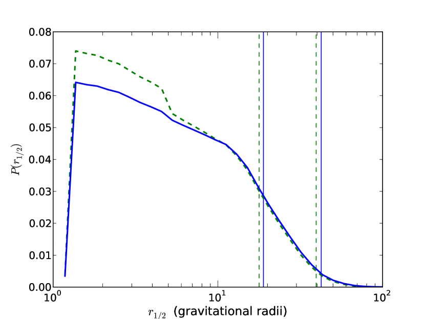
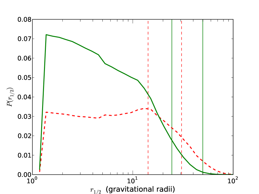
We followed the same procedure for the soft and hard bands, obtaining the joint probability distributions for $r_{s}$ shown in Figure 10. The expected values are $15.1\pm 12.6$ ($16.3\pm 14.7$) gravitational radii for the half-light radius of the soft (hard) band. For the average black hole mass in our sample, this translates into $0.42\pm 0.35$ ($0.46\pm 0.41$) light-days for the soft (hard) band. However, the probability distributions peak near $1R_{g}$, so only the upper limits are meaningful in practice. We get upper limits of $17.8$ ($18.9$) and $39.5$ ($42.4$) gravitational radii for the the soft (hard) band at $68\%$, and $95\%$ one-sided confidence limits, respectively, or $0.50$ ($0.53$) and $1.1$ ($1.2$) light-days for the the soft (hard) band at $68\%$, and $95\%$ one-sided confidence limits, respectively. The results are shown in Table 11, where the $99\%$ confidence values are also included.

When the calculations are performed on the full band, the expected value for the half-light radius is $14.1\pm 10.9$ gravitational radii ($0.40\pm 0.31$ light-days) and the $68\%$ probability upper limit on the half-light radius is $16.8$ gravitational radii ($0.47$ light-days). For comparison purposes, we repeated the calculation ignoring the effects of temporal smoothing by using single-epoch histograms for $p\big{(}\Delta m_{\beta\alpha}\big{|}r_{s}\big{)}$ (Figure 11). For this case we obtained a expected value of $24.0\pm 17.7$, and a $68\%$ probability upper limit of $28.9$ gravitational radii. This illustrates the impact of neglecting the length of the observation campaigns. Treating our time averaged data as single-epoch data overestimates the source size by a factor $1.7$

5 Discussion

We have measured full, soft and hard band X-ray light curves for $6$ lensed quasars to look for microlensing by comparing the observed flux ratios with the ratios predicted by macro lens modeling. We have tested for energy-dependent variability in several ways: a $\chi^{2}$ fit to the light curves of quadruple lenses, a comparison between the microlensing amplitude RMS of the soft and hard bands, and estimates of the average source size in the full, hard and soft X-ray energy bands.

Our $\chi^{2}$ test for energy-dependent microlensing shows a lack of correlation between soft and hard band in 2 of the 4-image lenses. This can be explained by a size difference between emitting regions, but also by a lack of correlation in the time domain. The RMS of the microlensing variability between the hard and soft bands is significantly different for a number of image pairs, but the sign of the difference varies and shows no consistent pattern. If a higher RMS is interpreted as arising from a more compact hard X-ray source, then this picture is consistent with the recent review of a sample of $8$ lensed quasars by Chartas et al. (2016), where for some objects the hard X-ray emission regions seems to be more compact than the soft and in others the soft appears to be smaller. However, a physical interpretation of a higher RMS level of microlensing variability in one band might not be straightforward, as suggested by the inconsistencies shown in Table 2 among image pairs of the same quadruple objects. An analysis on this question is in preparation (Guerras et al. 2017).

Our estimates of the average source size indicate that any size difference between the hard and soft emitting regions must be modest. This is in good agreement with the general picture that emerges from fully time-dependent studies of individual objects. Blackburne et al. (2015) found the same upper limit for the size of the hard and soft X-ray emitting regions in HE 1104$-$1805, as did Morgan et al. (2012) for QJ 0158$-$4325. Mosquera et al. (2013) could find only “weak evidence” that the hard X-ray emitting region in Q 2237+030 was more compact than the soft X-ray emitting region, and in HE 0435$-$1223 Blackburne et al. (2014) found no evidence for a size difference. The physical structure of what is believed to be a hot corona responsible for the X-ray continuum in quasars is poorly understood, and there are other astrophysical examples where hotter does not necessary equal smaller (e.g., the Solar corona). There is even some evidence (Chartas et al., 2012) suggesting that the soft emitting region could be more compact at least in one case.

The X-ray light curves span time intervals comparable to typical microlensing time scales, Treating them as single-epoch observations would result in overestimated source sizes. One way to address this problem is with fully time dependent calculations (Kochanek, 2004), but these are very computationally expensive. Here we introduce a simple approximation which at least avoids the bias of the single epoch method. This approximation essentially consists of introducing probability distribution modelled from time averaged tracks across the magnification patterns instead of isolated data points. The size estimates are consistently smaller using this approach. If we do not include the effects of time averaging, the source size estimate increases by a factor of $1.7$, which is a significant bias in the size estimate.

We also introduced a radial model for the microlensing optical depth based upon the best fit to real data given by Oguri et al. (2014). This model is simpler than the de Vaucouleurs stellar distribution plus NFW dark-matter halo used in previous time-dependent studies on individual objects (e.g., Morgan et al., 2008; Dai et al., 2010), yet it is an improvement with respect to using a uniform value in previous single-epoch studies over a heterogeneous sample of quasars (e.g., Guerras et al., 2013b; Jiménez-Vicente et al., 2015), where it is desirable to do the least possible assumptions on the lens galaxies to give a uniform treatment to all objects in the sample.

We also find a functional relationship between the RMS and the average value of the microlensing amplitude. This suggest that both observables carry physical information (e.g., about the quasar source size or the optical depth in galactic halos), and a more detailed analysis of this correlation is in preparation (Guerras et al. 2017). These two observables could be used complementarily to constraint physical properties from microlensing variability for a better understanding of lensed quasars.

6 Acknowledgements

We thank Jorge Jiménez-Vicente for useful discussions about the magnification patterns. We thank Evencio Mediavilla for providing an implementation of the Inverse Polygon Mapping code, and Masamune Oguri for providing the convergence and shear values of SDSS 1004+4112 calculated from his mass model. We would like to thank the anonymous reviewer for the useful comments and suggestions provided.

Support for this work was provided by the National Aeronautics and Space Administration through Chandra Award Number GO0- 11121A/B/C/D, GO1-12139A/B/C, GO2-13132A/B/C, and G03-14110A/B/C issued by the Chandra X-ray Observatory Center, which is operated by the Smithsonian Astrophysical Observatory for and on behalf of the National Aeronautics Space Administration under contract NAS8-03060. XD acknowledges NASA ADAP program NNX15AF04G and NSF grant AST–1413056. CSK is supported by NSF grant AST-1515876.

Figure 1: Stacked images of the objects in the sample. Note that the angular scale is not uniform.

Figure 2: Flux ratios for QJ 0158$-$4325 on a magnitude scale. Continuous blue (dashed green) curves show the hard (soft) emission. The orange dashed horizontal lines represent the baseline ratios.

Figure 3: Flux ratios for HE 0435$-$1223 on a magnitude scale. Continuous blue (dashed green) curves show the hard (soft) emission. The orange dashed horizontal lines represent the baseline ratios.

Figure 4: Flux ratios for SDSS 0924+0219 on a magnitude scale. Continuous blue (dashed green) curves show the hard (soft) emission. The orange dashed horizontal lines represent the baseline ratios.

Figure 5: Flux ratios for SDSS 1004+4112 on a magnitude scale. Continuous blue (dashed green) curves show the hard (soft) emission. The orange dashed horizontal lines represent the baseline ratios.

Figure 6: Flux ratios for HE 1104$-$1805 on a magnitude scale. Continuous blue (dashed green) curves show the hard (soft) emission. The orange dashed horizontal lines represent the baseline ratios.

Figure 7: Flux ratios for Q 2237+0305 on a magnitude scale. Continuous blue (dashed green) curves show the hard (soft) emission. The orange dashed horizontal lines represent the baseline ratios.

Figure 8: The empirical relationship between the RMS (root-mean-square) and mean of the full band microlensing amplitude (defined in Eq. 5). The best linear fit in log space is shown by a solid line. Given the extraordinarily long campaign for Q 2237+0305, its data have been broken in $3$ chunks of approximately equal size to roughly match the other objects.

Figure 9: Probability Density Functions of differential microlensing between image $C$ and $A$ of Q 2237+0305 for a source with a half-light radius of $0.5$ light-day. The solid, green thick line shows the distribution function obtained from $10^{8}$ simulated observation campaigns spanning $1.7$ $R_{E}$ each with $30$ observations, which roughly matches our observations. The dashed, red thick line shows the analogous distribution from $10^{8}$ simple single-epoch observations. The results for intermediate track lengths of $0.05$, $0.10$, $0.20$, $0.50$, and $1.00$ $R_{E}$ (thin solid lines) are also shown. The longer the averaged light curves, the higher the departure from a single-epoch probability distribution.

Figure 10: Joint probability distribution for the average half-light radius. The hard (soft) X-ray band result is shown by the continuous blue (dashed green) curve. The vertical lines show the corresponding $68\%$ and $95\%$ one-sided probability upper limits.

Figure 11: Joint probability distribution for the average half-light radius of the full X-ray band (continuous green). Using single-epoch histograms neglects the effect of temporal smoothing, and the resulting distribution (dashed red) yields overestimated source sizes. The vertical lines show the corresponding $68\%$ and $95\%$ one-sided probability upper limits.

Table 1: Lens Data

Object	$z_{s}$	$z_{l}$	$R_{E}$	$t_{E}$	$t_{s}$	$\Delta t_{obs}$	$\Delta t_{obs}/t_{E}$	$M_{BH}$
			(light-days)	(years)	(years)	(years)	(Einstein radii)	($\times 10^{9}$ $M_{\odot}$)
QJ 0158$-$4325	1.29	0.317	7.434	18.0	0.86	4.6	0.26	$0.16$ (MgII)
HE 0435$-$1223	1.689	0.46	7.986	18.3	0.47	7.3	0.40	$0.50$ (CIV)
SDSS 0924+0219	1.524	0.39	7.790	20.4	0.39	5.6	0.27	$0.11$ (MgII)
SDSS 1004+4112	1.734	0.68	7.737	28.9	0.28	9.4	0.33	$0.39$ (MgII)
HE 1104$-$1805	2.32	0.73	8.244	21.7	2.23	14.5	0.67	$0.59$ (Hβ)
Q 2237+0305	1.69	0.0395	3.660	8.11	0.23	13.6	1.68	$1.20$ (Hβ)

Note. — Based on the source and lens redshifts $z_{s}$ and $z_{l}$, the Einstein radius $R_{E}$ can be computed. Here we report the estimates given by Mosquera & Kochanek (2011) of $R_{E}$ as well as the Einstein radius and source crossing time scales $t_{E}$ and $t_{s}$, assuming a mean stellar mass in lens galaxies of $\langle M_{*}\rangle=0.3$ $M_{\odot}$, for comparison to the time span of the observations $\Delta t_{obs}$. The last column reports the estimated black hole mass and the emission lines used for the estimates by Morgan et al. (2010) (QJ 0158$-$4325, HE 0435$-$1223, SDSS 1004+4112), Peng et al. (2006) (SDSS 0924+0219) and Assef et al. (2011) (HE 1104$-$1805, Q 2237+0305).

Table 2: RMS microlensing variability

Object	Pair	N	RMS, full	RMS, hard	RMS, soft	p-value
QJ 0158$-$4325	B/A	$12$	$0.167\pm 0.049$	$0.216\pm 0.072$	$0.216\pm 0.067$	$1.00$
HE 1104$-$1805	B/A	$15$	$2.019\pm 0.362$	$1.934\pm 0.521$	$2.765\pm 0.776$	$<0.01$
HE 0435$-$1223	B/A	$10$	$0.216\pm 0.049$	$0.234\pm 0.073$	$0.215\pm 0.069$	$0.56$
HE 0435$-$1223	C/A	$10$	$0.224\pm 0.043$	$0.276\pm 0.080$	$0.169\pm 0.050$	$<0.01$
HE 0435$-$1223	D/A	$10$	$0.342\pm 0.067$	$0.272\pm 0.096$	$0.364\pm 0.093$	$0.04$
SDSS 0924+0219	B/A	$6$	$0.260\pm 0.073$	$0.241\pm 0.092$	$0.200\pm 0.075$	$0.42$
SDSS 0924+0219	C/A	$6$	$0.091\pm 0.039$	$0.043\pm 0.046$	$0.126\pm 0.050$	$0.01$
SDSS 0924+0219	D/A	$6$	$0.045\pm 0.018$	$0.087\pm 0.045$	$0.065\pm 0.027$	$0.34$
SDSS 1004+4112	B/A	$11$	$0.834\pm 0.111$	$0.792\pm 0.136$	$1.032\pm 0.167$	$<0.01$
SDSS 1004+4112	C/A	$11$	$1.914\pm 0.524$	$1.766\pm 0.642$	$2.149\pm 0.733$	$0.21$
SDSS 1004+4112	D/A	$11$	$3.272\pm 0.802$	$3.022\pm 1.036$	$3.821\pm 1.110$	$0.10$
Q 2237+0305	B/A	$30$	$0.114\pm 0.025$	$0.147\pm 0.031$	$0.108\pm 0.027$	$<0.01$
Q 2237+0305	C/A	$30$	$0.264\pm 0.024$	$0.308\pm 0.037$	$0.265\pm 0.031$	$<0.01$
Q 2237+0305	D/A	$30$	$0.182\pm 0.014$	$0.196\pm 0.021$	$0.224\pm 0.035$	$<0.01$

Table 3: Absorption-corrected count rates for QJ 0158$-$4325.

ObsId	Date	Exp	$\rm{A_{full}}$	$\rm{A_{soft}}$	$\rm{A_{hard}}$	$\rm{B_{full}}$	$\rm{B_{soft}}$	$\rm{B_{hard}}$
11556	2009-Nov-06	$5.03$	$23.7^{+3.2}_{-6.6}$	$13.9^{+2.6}_{-2.5}$	$9.7^{+1.8}_{-1.9}$	$10.2^{+4.2}_{-2.6}$	$9.3^{+2.4}_{-2.2}$	$2.2^{+0.8}_{-0.7}$
11557	2010-Jan-12	$5.02$	$27.3^{+4.1}_{-2.8}$	$19.8^{+3.0}_{-3.3}$	$8.9^{+1.7}_{-1.6}$	$13.6^{+2.5}_{-2.1}$	$10.9^{+1.9}_{-2.2}$	$4.0^{+1.2}_{-0.9}$
11558	2010-Mar-10	$5.04$	$29.4^{+3.9}_{-4.4}$	$20.5^{+5.4}_{-2.9}$	$8.0^{+2.1}_{-1.8}$	$11.0^{+2.3}_{-2.0}$	$7.4^{+1.7}_{-1.3}$	$4.2^{+1.3}_{-0.9}$
11559	2010-May-23	$4.94$	$32.6^{+2.9}_{-3.9}$	$21.7^{+3.0}_{-2.9}$	$10.5^{+1.8}_{-2.2}$	$8.5^{+1.6}_{-1.5}$	$6.1^{+1.5}_{-1.3}$	$3.2^{+0.9}_{-1.0}$
11560	2010-Jul-28	$4.95$	$32.6^{+2.9}_{-3.7}$	$20.7^{+2.6}_{-3.3}$	$10.1^{+2.4}_{-1.6}$	$9.3^{+1.7}_{-1.7}$	$7.2^{+1.6}_{-1.6}$	$2.6^{+1.0}_{-0.8}$
11561	2010-Oct-06	$4.95$	$26.1^{+3.0}_{-3.4}$	$20.1^{+2.4}_{-3.1}$	$7.3^{+1.9}_{-1.8}$	$12.1^{+1.8}_{-1.8}$	$10.2^{+1.9}_{-2.3}$	$2.7^{+1.0}_{-0.8}$
14483	2013-Mar-26	$18.6$	$23.5^{+1.4}_{-4.2}$	$15.0^{+1.1}_{-5.0}$	$8.9^{+0.8}_{-1.2}$	$6.5^{+0.7}_{-0.7}$	$5.3^{+0.7}_{-0.7}$	$1.8^{+0.4}_{-0.3}$
14484	2013-Apr-24	$18.6$	$19.9^{+1.5}_{-2.1}$	$14.1^{+1.0}_{-1.1}$	$6.9^{+0.7}_{-0.7}$	$6.7^{+0.7}_{-1.4}$	$4.7^{+0.7}_{-0.7}$	$2.4^{+0.4}_{-0.4}$
14485	2013-Dec-05	$18.6$	$26.9^{+1.7}_{-5.0}$	$18.1^{+2.4}_{-2.3}$	$9.4^{+0.9}_{-1.3}$	$6.6^{+2.2}_{-0.7}$	$4.6^{+0.8}_{-0.8}$	$2.1^{+0.4}_{-0.4}$
14486	2013-Dec-29	$18.6$	$22.8^{+2.3}_{-2.1}$	$13.9^{+1.1}_{-1.2}$	$9.2^{+1.2}_{-1.4}$	$9.7^{+1.0}_{-0.9}$	$6.8^{+0.8}_{-0.7}$	$3.5^{+0.6}_{-0.5}$
14487	2014-May-30	$18.6$	$37.2^{+1.5}_{-1.6}$	$23.1^{+1.5}_{-2.0}$	$13.7^{+1.1}_{-1.5}$	$9.9^{+0.9}_{-0.9}$	$6.9^{+0.8}_{-0.7}$	$3.3^{+0.6}_{-0.6}$
14488	2014-Jun-11	$18.6$	$30.8^{+2.1}_{-4.7}$	$21.6^{+2.9}_{-5.9}$	$10.2^{+1.6}_{-1.2}$	$10.4^{+2.6}_{-1.6}$	$7.2^{+2.6}_{-2.6}$	$4.4^{+0.7}_{-0.7}$

Note. — Count rates are in units of $10^{-3}\,{\rm s}^{-1}$. Exp reports the values stored in the header keyword EXPOSURE in units of $10^{3}\,{\rm s}$

Table 4: Absorption-corrected count rates for HE 0435$-$1223.

ObsId	Date	Exp	$\rm{A_{full}}$	$\rm{A_{soft}}$	$\rm{A_{hard}}$	$\rm{B_{full}}$	$\rm{B_{soft}}$	$\rm{B_{hard}}$	$\rm{C_{full}}$	$\rm{C_{soft}}$	$\rm{C_{hard}}$	$\rm{D_{full}}$	$\rm{D_{soft}}$	$\rm{D_{hard}}$
7761	2006-Dec-17	$10.0$	$28.1^{+2.7}_{-3.4}$	$17.8^{+2.1}_{-1.9}$	$10.0^{+3.4}_{-1.2}$	$9.5^{+1.8}_{-1.2}$	$7.5^{+1.2}_{-1.2}$	$3.2^{+0.7}_{-0.7}$	$9.0^{+1.7}_{-1.1}$	$6.9^{+1.1}_{-1.1}$	$3.8^{+0.7}_{-0.7}$	$8.6^{+1.7}_{-1.0}$	$5.4^{+0.9}_{-0.8}$	$4.6^{+0.8}_{-1.4}$
11550	2009-Dec-07	$12.9$	$8.4^{+1.1}_{-1.0}$	$5.3^{+1.0}_{-1.1}$	$3.9^{+0.6}_{-0.6}$	$9.7^{+1.2}_{-1.4}$	$6.2^{+1.1}_{-1.2}$	$3.7^{+0.7}_{-0.5}$	$10.1^{+1.2}_{-1.2}$	$5.4^{+1.7}_{-0.8}$	$4.1^{+0.8}_{-0.6}$	$8.6^{+1.0}_{-1.1}$	$5.4^{+1.0}_{-0.9}$	$2.9^{+0.6}_{-0.5}$
11551	2010-Jul-05	$12.8$	$7.8^{+1.1}_{-0.9}$	$4.6^{+0.8}_{-1.0}$	$3.8^{+0.6}_{-0.7}$	$7.0^{+0.9}_{-0.9}$	$4.1^{+0.8}_{-1.0}$	$3.1^{+0.8}_{-0.5}$	$8.2^{+1.1}_{-1.0}$	$3.6^{+1.0}_{-0.7}$	$4.5^{+0.9}_{-0.7}$	$7.4^{+1.0}_{-0.9}$	$4.5^{+0.9}_{-0.8}$	$3.4^{+0.8}_{-0.6}$
11552	2010-Oct-30	$12.8$	$5.2^{+1.0}_{-0.8}$	$3.0^{+0.7}_{-0.7}$	$2.4^{+0.6}_{-0.5}$	$4.5^{+0.9}_{-0.8}$	$1.8^{+0.5}_{-0.5}$	$2.8^{+0.6}_{-0.5}$	$5.6^{+0.9}_{-0.8}$	$2.1^{+0.7}_{-0.5}$	$3.4^{+0.7}_{-0.6}$	$4.8^{+0.8}_{-0.7}$	$2.4^{+0.8}_{-0.6}$	$2.4^{+0.5}_{-0.4}$
14489	2012-Nov-28	$37.2$	$11.7^{+0.6}_{-0.8}$	$7.5^{+1.2}_{-1.2}$	$4.7^{+0.9}_{-0.5}$	$7.2^{+0.5}_{-0.6}$	$4.5^{+0.5}_{-0.9}$	$2.8^{+0.4}_{-0.4}$	$10.0^{+0.6}_{-0.6}$	$5.7^{+1.6}_{-0.7}$	$4.7^{+0.8}_{-0.7}$	$8.5^{+0.7}_{-0.6}$	$4.1^{+1.3}_{-0.5}$	$4.2^{+0.4}_{-0.5}$
14490	2013-Apr-01	$36.2$	$11.6^{+0.6}_{-2.3}$	$8.1^{+0.9}_{-0.8}$	$4.6^{+0.4}_{-0.4}$	$7.3^{+0.5}_{-2.1}$	$4.4^{+0.6}_{-0.5}$	$2.9^{+0.3}_{-0.3}$	$10.7^{+2.8}_{-2.1}$	$6.9^{+0.7}_{-0.7}$	$4.5^{+0.4}_{-0.4}$	$6.3^{+0.5}_{-1.5}$	$4.3^{+0.5}_{-0.5}$	$2.7^{+0.3}_{-0.3}$
14491	2013-Aug-14	$36.2$	$11.9^{+0.7}_{-0.8}$	$7.8^{+0.6}_{-0.8}$	$6.0^{+0.4}_{-0.6}$	$6.7^{+0.5}_{-0.6}$	$3.5^{+0.5}_{-0.4}$	$2.9^{+0.4}_{-0.3}$	$9.5^{+0.8}_{-0.9}$	$5.1^{+0.6}_{-0.5}$	$4.0^{+0.5}_{-0.4}$	$9.0^{+0.6}_{-2.5}$	$4.9^{+0.6}_{-0.6}$	$3.8^{+0.5}_{-0.4}$
14492	2013-Sep-22	$35.5$	$10.6^{+0.8}_{-0.9}$	$5.8^{+0.7}_{-0.6}$	$4.8^{+1.3}_{-1.1}$	$5.6^{+1.8}_{-0.5}$	$3.6^{+0.5}_{-0.5}$	$2.5^{+1.1}_{-0.3}$	$8.2^{+0.8}_{-0.6}$	$5.4^{+0.5}_{-0.9}$	$3.6^{+0.4}_{-0.8}$	$6.3^{+0.4}_{-0.4}$	$4.0^{+0.5}_{-0.5}$	$2.9^{+0.4}_{-0.6}$
14493	2014-Mar-08	$36.2$	$11.6^{+1.0}_{-0.8}$	$6.5^{+1.2}_{-1.0}$	$5.7^{+0.7}_{-0.6}$	$6.3^{+0.5}_{-0.5}$	$3.4^{+0.5}_{-0.7}$	$3.0^{+0.4}_{-0.4}$	$11.1^{+0.8}_{-1.0}$	$5.7^{+0.6}_{-0.8}$	$5.2^{+0.5}_{-0.6}$	$6.1^{+0.5}_{-0.5}$	$2.8^{+0.4}_{-0.4}$	$3.3^{+0.3}_{-0.3}$
14494	2014-Apr-10	$36.2$	$9.9^{+0.9}_{-0.8}$	$5.4^{+0.6}_{-0.5}$	$4.8^{+0.4}_{-0.4}$	$6.8^{+0.7}_{-0.7}$	$4.3^{+0.5}_{-0.5}$	$3.4^{+0.3}_{-0.3}$	$8.4^{+0.7}_{-0.7}$	$4.9^{+0.5}_{-0.5}$	$3.9^{+0.4}_{-0.4}$	$7.2^{+0.6}_{-0.7}$	$4.6^{+0.4}_{-0.4}$	$3.1^{+0.4}_{-0.4}$

Note. — Count rates are in units of $10^{-3}\,{\rm s}^{-1}$. Exp reports the values stored in the header keyword EXPOSURE in units of $10^{3}\,{\rm s}$

Table 5: Absorption-corrected count rates for SDSS 0924+0219.

ObsId	Date	Exp	$\rm{A_{full}}$	$\rm{A_{soft}}$	$\rm{A_{hard}}$	$\rm{B_{full}}$	$\rm{B_{soft}}$	$\rm{B_{hard}}$	$\rm{C_{full}}$	$\rm{C_{soft}}$	$\rm{C_{hard}}$	$\rm{D_{full}}$	$\rm{D_{soft}}$	$\rm{D_{hard}}$
5604	2005-Feb-24	$18.0$	$4.6^{+1.2}_{-0.6}$	$3.5^{+0.8}_{-0.7}$	$1.5^{+0.6}_{-0.3}$	$1.7^{+0.4}_{-0.4}$	$1.3^{+0.4}_{-0.3}$	$0.4^{+0.2}_{-0.2}$	$0.7^{+0.2}_{-0.2}$	$0.5^{+0.2}_{-0.2}$	$0.1^{+0.1}_{-0.1}$	$0.6^{+0.3}_{-0.2}$	$0.6^{+0.3}_{-0.2}$	$0.1^{+0.1}_{-0.1}$
11562	2010-Jan-13	$21.5$	$10.1^{+1.3}_{-1.6}$	$8.2^{+0.8}_{-1.8}$	$2.7^{+0.5}_{-0.4}$	$2.5^{+0.6}_{-0.5}$	$1.7^{+0.3}_{-0.3}$	$0.8^{+0.3}_{-0.2}$	$0.6^{+0.2}_{-0.2}$	$0.6^{+0.2}_{-0.2}$	$0.1^{+0.1}_{-0.1}$	$1.7^{+0.4}_{-0.4}$	$1.5^{+0.4}_{-0.3}$	$0.4^{+0.2}_{-0.2}$
11563	2010-Mar-11	$21.3$	$6.8^{+0.7}_{-1.1}$	$4.2^{+0.8}_{-0.6}$	$2.2^{+0.5}_{-0.5}$	$0.7^{+0.2}_{-0.2}$	$0.5^{+0.2}_{-0.2}$	$0.3^{+0.2}_{-0.1}$	$0.8^{+0.3}_{-0.2}$	$0.8^{+0.3}_{-0.2}$	$0.1^{+0.1}_{-0.1}$	$0.7^{+0.3}_{-0.2}$	$0.9^{+0.3}_{-0.3}$	$0.1^{+0.1}_{-0.1}$
11564	2010-May-10	$21.6$	$16.0^{+1.0}_{-1.0}$	$10.7^{+1.2}_{-1.4}$	$5.0^{+0.7}_{-0.8}$	$2.3^{+0.4}_{-0.3}$	$1.9^{+0.4}_{-0.3}$	$0.7^{+0.2}_{-0.2}$	$0.8^{+0.2}_{-0.2}$	$0.4^{+0.2}_{-0.1}$	$0.4^{+0.2}_{-0.1}$	$1.1^{+0.3}_{-0.3}$	$0.7^{+0.3}_{-0.2}$	$0.3^{+0.2}_{-0.1}$
11565	2010-Jun-23	$21.6$	$10.2^{+2.1}_{-1.0}$	$7.7^{+1.1}_{-1.0}$	$3.7^{+0.5}_{-0.6}$	$4.1^{+0.6}_{-0.9}$	$2.5^{+0.5}_{-0.5}$	$1.5^{+0.4}_{-0.3}$	$0.7^{+0.3}_{-0.2}$	$0.4^{+0.2}_{-0.1}$	$0.2^{+0.1}_{-0.1}$	$0.9^{+0.5}_{-0.3}$	$0.8^{+0.3}_{-0.2}$	$0.2^{+0.2}_{-0.1}$
11566	2010-Oct-06	$21.5$	$7.1^{+1.7}_{-0.7}$	$5.9^{+0.7}_{-1.0}$	$2.4^{+0.4}_{-0.8}$	$2.0^{+0.5}_{-0.4}$	$1.6^{+0.5}_{-0.3}$	$0.4^{+0.4}_{-0.1}$	$0.7^{+0.3}_{-0.3}$	$0.5^{+0.2}_{-0.2}$	$0.2^{+0.3}_{-0.1}$	$1.1^{+0.4}_{-0.3}$	$0.5^{+0.3}_{-0.2}$	$0.6^{+0.4}_{-0.2}$

Note. — Count rates are in units of $10^{-3}\,{\rm s}^{-1}$. Exp reports the values stored in the header keyword EXPOSURE in units of $10^{3}\,{\rm s}$

Table 6: Absorption-corrected count rates for SDSS 1004+4112.

ObsId	Date	Exp	$\rm{A_{full}}$	$\rm{A_{soft}}$	$\rm{A_{hard}}$	$\rm{B_{full}}$	$\rm{B_{soft}}$	$\rm{B_{hard}}$	$\rm{C_{full}}$	$\rm{C_{soft}}$	$\rm{C_{hard}}$	$\rm{D_{full}}$	$\rm{D_{soft}}$	$\rm{D_{hard}}$
11556	2005-Jan-02	$80.1$	$16.9{\pm 0.5}$	$10.5{\pm 0.4}$	$7.0{\pm 0.3}$	$21.6{\pm 0.5}$	$13.6{\pm 0.4}$	$8.4{\pm 0.3}$	$17.6{\pm 0.5}$	$10.6{\pm 0.4}$	$7.2{\pm 0.3}$	$9.9{\pm 0.4}$	$5.8{\pm 0.3}$	$4.3{\pm 0.2}$
11557	2010-Mar-08	$5.96$	$11.4{\pm 1.4}$	$5.5{\pm 1.0}$	$6.1{\pm 1.0}$	$16.0{\pm 1.7}$	$10.8{\pm 1.4}$	$5.5{\pm 1.0}$	$12.0{\pm 1.4}$	$6.2{\pm 1.1}$	$5.8{\pm 1.0}$	$15.3{\pm 1.6}$	$10.5{\pm 1.4}$	$5.1{\pm 0.9}$
11558	2010-Jun-19	$5.96$	$8.8{\pm 1.3}$	$5.5{\pm 1.0}$	$3.6{\pm 0.8}$	$8.6{\pm 1.2}$	$5.1{\pm 1.0}$	$3.6{\pm 0.8}$	$17.0{\pm 1.7}$	$10.2{\pm 1.4}$	$7.1{\pm 1.1}$	$11.0{\pm 1.4}$	$6.2{\pm 1.1}$	$4.9{\pm 0.9}$
11559	2010-Sep-23	$5.96$	$9.2{\pm 1.3}$	$4.7{\pm 1.0}$	$4.6{\pm 0.9}$	$12.0{\pm 1.4}$	$5.9{\pm 1.0}$	$6.3{\pm 1.0}$	$11.4{\pm 1.4}$	$6.2{\pm 1.1}$	$5.3{\pm 1.0}$	$8.3{\pm 1.2}$	$4.1{\pm 0.9}$	$4.3{\pm 0.9}$
11560	2011-Jan-30	$5.96$	$5.3{\pm 1.0}$	$2.8{\pm 0.7}$	$2.6{\pm 0.7}$	$7.9{\pm 1.2}$	$4.0{\pm 0.9}$	$4.0{\pm 0.8}$	$19.6{\pm 1.8}$	$10.7{\pm 1.4}$	$9.2{\pm 1.2}$	$14.4{\pm 1.6}$	$7.8{\pm 1.2}$	$6.8{\pm 1.1}$
11561	2013-Jan-28	$24.7$	$9.0{\pm 0.6}$	$4.1{\pm 0.4}$	$5.0{\pm 0.5}$	$19.4{\pm 0.9}$	$10.5{\pm 0.7}$	$9.1{\pm 0.6}$	$14.6{\pm 0.8}$	$7.4{\pm 0.6}$	$7.4{\pm 0.5}$	$8.2{\pm 0.6}$	$4.3{\pm 0.4}$	$4.0{\pm 0.4}$
14483	2013-Mar-01	$24.7$	$9.4{\pm 0.6}$	$4.7{\pm 0.5}$	$4.9{\pm 0.5}$	$19.9{\pm 0.9}$	$10.5{\pm 0.7}$	$9.6{\pm 0.6}$	$15.2{\pm 0.8}$	$7.5{\pm 0.6}$	$7.9{\pm 0.6}$	$7.0{\pm 0.5}$	$3.4{\pm 0.4}$	$3.6{\pm 0.4}$
14484	2013-Oct-05	$24.1$	$10.2{\pm 0.7}$	$4.9{\pm 0.5}$	$5.4{\pm 0.5}$	$16.9{\pm 0.9}$	$9.1{\pm 0.6}$	$8.0{\pm 0.6}$	$15.4{\pm 0.8}$	$7.4{\pm 0.6}$	$8.1{\pm 0.6}$	$6.0{\pm 0.5}$	$3.1{\pm 0.4}$	$3.0{\pm 0.4}$
14485	2013-Nov-16	$23.8$	$8.9{\pm 0.6}$	$4.0{\pm 0.4}$	$5.0{\pm 0.5}$	$17.4{\pm 0.9}$	$9.4{\pm 0.7}$	$8.2{\pm 0.6}$	$17.3{\pm 0.9}$	$9.7{\pm 0.7}$	$7.8{\pm 0.6}$	$10.3{\pm 0.7}$	$4.7{\pm 0.5}$	$5.6{\pm 0.5}$
14486	2014-Apr-30	$23.3$	$8.0{\pm 0.6}$	$4.1{\pm 0.5}$	$4.1{\pm 0.4}$	$14.1{\pm 0.8}$	$6.9{\pm 0.6}$	$7.3{\pm 0.6}$	$10.8{\pm 0.7}$	$5.7{\pm 0.5}$	$5.2{\pm 0.5}$	$5.3{\pm 0.5}$	$2.3{\pm 0.3}$	$3.0{\pm 0.4}$
14487	2014-Jun-02	$24.7$	$7.1{\pm 0.6}$	$3.2{\pm 0.4}$	$4.0{\pm 0.4}$	$20.8{\pm 0.9}$	$9.9{\pm 0.7}$	$11.1{\pm 0.7}$	$11.5{\pm 0.7}$	$5.2{\pm 0.5}$	$6.3{\pm 0.5}$	$4.5{\pm 0.4}$	$2.1{\pm 0.3}$	$2.4{\pm 0.3}$

Note. — Count rates are in units of $10^{-3}\,{\rm s}^{-1}$. Exp reports the values stored in the header keyword EXPOSURE in units of $10^{3}\,{\rm s}$

Table 7: Absorption-corrected count rates for HE 1104$-$1805.

ObsId	Date	Exp	$\rm{A_{full}}$	$\rm{A_{soft}}$	$\rm{A_{hard}}$	$\rm{B_{full}}$	$\rm{B_{soft}}$	$\rm{B_{hard}}$
375	2000-Jun-11	$47.4$	$21.5^{+0.9}_{-1.0}$	$13.6^{+0.7}_{-0.7}$	$10.2^{+0.6}_{-0.7}$	$12.0^{+0.5}_{-0.5}$	$8.2^{+0.6}_{-0.6}$	$4.6^{+0.4}_{-0.4}$
6917	2006-Mar-15	$4.55$	$8.0^{+2.5}_{-1.6}$	$3.6^{+1.2}_{-1.3}$	$6.0^{+1.3}_{-1.2}$	$12.3^{+2.3}_{-2.5}$	$8.8^{+1.8}_{-2.5}$	$6.2^{+1.3}_{-1.2}$
6918	2006-Feb-16	$4.96$	$7.8^{+1.4}_{-1.4}$	$2.9^{+1.3}_{-0.8}$	$4.2^{+1.2}_{-1.3}$	$17.5^{+2.3}_{-2.9}$	$6.1^{+2.0}_{-1.1}$	$9.8^{+1.9}_{-2.1}$
6919	2006-Apr-09	$4.87$	$7.2^{+1.4}_{-1.8}$	$2.8^{+1.1}_{-1.0}$	$4.4^{+1.1}_{-1.1}$	$12.0^{+2.1}_{-2.8}$	$8.0^{+1.6}_{-2.2}$	$5.7^{+1.3}_{-1.8}$
6920	2006-Oct-31	$5.01$	$12.6^{+1.9}_{-2.1}$	$5.6^{+1.9}_{-1.4}$	$5.8^{+1.4}_{-0.9}$	$7.4^{+1.7}_{-1.5}$	$4.7^{+1.5}_{-1.1}$	$3.0^{+1.0}_{-0.7}$
6921	2006-Nov-08	$4.92$	$10.9^{+2.1}_{-1.8}$	$5.2^{+1.6}_{-1.5}$	$6.0^{+1.4}_{-1.1}$	$9.3^{+1.8}_{-1.5}$	$5.3^{+1.5}_{-1.4}$	$4.8^{+1.4}_{-1.0}$
11553	2010-Feb-09	$12.8$	$8.7^{+1.0}_{-1.2}$	$3.8^{+1.0}_{-0.7}$	$4.3^{+1.1}_{-0.7}$	$12.6^{+1.1}_{-1.2}$	$5.7^{+1.3}_{-1.1}$	$6.5^{+1.1}_{-1.2}$
11554	2010-Jul-12	$12.8$	$19.7^{+1.9}_{-3.8}$	$8.8^{+1.4}_{-1.9}$	$12.1^{+1.2}_{-1.6}$	$7.8^{+1.3}_{-1.7}$	$3.8^{+0.7}_{-1.3}$	$4.5^{+0.7}_{-0.7}$
11555	2010-Dec-20	$12.8$	$10.2^{+1.0}_{-1.2}$	$4.0^{+1.1}_{-0.8}$	$5.7^{+1.0}_{-0.9}$	$11.7^{+1.3}_{-1.3}$	$5.1^{+1.3}_{-1.1}$	$6.3^{+1.1}_{-0.9}$
14501	2013-Mar-01	$13.7$	$8.1^{+1.0}_{-1.0}$	$2.9^{+0.6}_{-0.5}$	$5.3^{+0.7}_{-0.7}$	$7.1^{+0.9}_{-0.8}$	$2.7^{+0.7}_{-0.5}$	$4.8^{+0.7}_{-0.7}$
14502	2013-Jul-26	$13.7$	$7.1^{+0.8}_{-1.4}$	$2.3^{+0.6}_{-0.4}$	$4.6^{+0.6}_{-1.2}$	$11.3^{+1.2}_{-1.7}$	$4.5^{+0.9}_{-0.7}$	$6.6^{+0.9}_{-1.3}$
14503	2013-Dec-08	$12.8$	$6.3^{+1.0}_{-0.8}$	$2.6^{+0.9}_{-0.5}$	$3.7^{+0.7}_{-0.5}$	$5.8^{+0.8}_{-0.7}$	$2.8^{+0.8}_{-0.7}$	$3.3^{+0.6}_{-0.5}$
14504	2014-Mar-25	$13.7$	$10.6^{+1.2}_{-1.2}$	$3.8^{+0.7}_{-2.4}$	$6.7^{+0.9}_{-0.8}$	$8.7^{+0.9}_{-1.1}$	$3.2^{+0.7}_{-1.2}$	$5.3^{+0.8}_{-0.8}$
14505	2014-Jul-14	$13.7$	$13.0^{+1.5}_{-1.9}$	$5.0^{+0.7}_{-1.3}$	$9.2^{+0.9}_{-1.5}$	$6.2^{+1.7}_{-0.8}$	$2.7^{+0.6}_{-0.7}$	$4.3^{+0.6}_{-0.6}$
14506	2014-Dec-02	$13.7$	$4.7^{+0.7}_{-0.8}$	$1.5^{+0.5}_{-0.4}$	$3.0^{+0.6}_{-0.4}$	$7.1^{+1.1}_{-1.4}$	$2.8^{+0.7}_{-0.5}$	$3.7^{+0.8}_{-0.5}$

Note. — Count rates are in units of $10^{-3}\,{\rm s}^{-1}$. Exp reports the values stored in the header keyword EXPOSURE in units of $10^{3}\,{\rm s}$

Table 8: Absorption-corrected count rates for Q 2237+0305.

ObsId	Date	Exp	$\rm{A_{full}}$	$\rm{A_{soft}}$	$\rm{A_{hard}}$	$\rm{B_{full}}$	$\rm{B_{soft}}$	$\rm{B_{hard}}$	$\rm{C_{full}}$	$\rm{C_{soft}}$	$\rm{C_{hard}}$	$\rm{D_{full}}$	$\rm{D_{soft}}$	$\rm{D_{hard}}$
431	2000-Sep-07	$30.3$	$56.7^{+2.1}_{-2.3}$	$53.4^{+3.8}_{-4.2}$	$18.7^{+2.3}_{-2.0}$	$9.9^{+0.7}_{-0.7}$	$9.6^{+1.0}_{-1.0}$	$3.4^{+0.4}_{-0.6}$	$22.8^{+1.2}_{-1.1}$	$25.9^{+1.5}_{-1.6}$	$6.9^{+2.0}_{-0.6}$	$9.3^{+0.7}_{-0.7}$	$8.6^{+1.8}_{-0.9}$	$3.2^{+0.9}_{-0.4}$
1632	2001-Dec-08	$9.54$	$43.0^{+3.5}_{-6.3}$	$36.7^{+4.3}_{-4.0}$	$16.7^{+1.6}_{-2.3}$	$7.7^{+2.0}_{-1.0}$	$8.7^{+1.5}_{-1.5}$	$2.4^{+0.6}_{-0.5}$	$13.2^{+1.8}_{-1.5}$	$12.1^{+2.3}_{-2.1}$	$5.8^{+1.0}_{-0.9}$	$7.8^{+1.2}_{-1.1}$	$8.1^{+1.5}_{-1.4}$	$2.5^{+0.6}_{-0.5}$
6831	2006-Jan-10	$7.27$	$20.2^{+2.0}_{-5.5}$	$14.4^{+2.7}_{-2.0}$	$8.4^{+1.3}_{-1.6}$	$14.3^{+1.8}_{-3.1}$	$8.1^{+1.7}_{-3.7}$	$7.3^{+1.3}_{-1.5}$	$5.1^{+1.1}_{-1.0}$	$3.7^{+1.3}_{-1.1}$	$2.2^{+0.7}_{-0.5}$	$7.0^{+3.2}_{-1.2}$	$6.9^{+1.6}_{-4.4}$	$2.7^{+0.9}_{-0.6}$
6832	2006-May-01	$7.94$	$35.7^{+6.9}_{-3.7}$	$29.2^{+5.0}_{-5.3}$	$15.4^{+2.3}_{-2.1}$	$16.8^{+2.3}_{-1.8}$	$12.5^{+2.3}_{-1.8}$	$7.6^{+1.3}_{-1.2}$	$16.3^{+2.1}_{-3.4}$	$14.9^{+2.9}_{-2.8}$	$5.5^{+0.9}_{-0.8}$	$12.1^{+1.7}_{-3.9}$	$8.5^{+2.0}_{-1.7}$	$4.6^{+1.0}_{-0.8}$
6833	2006-May-27	$7.95$	$21.1^{+3.0}_{-2.9}$	$17.6^{+2.9}_{-3.8}$	$7.9^{+1.7}_{-1.2}$	$7.7^{+1.5}_{-1.2}$	$5.9^{+1.7}_{-1.5}$	$3.5^{+1.1}_{-0.7}$	$8.6^{+1.5}_{-1.6}$	$6.8^{+1.8}_{-2.1}$	$3.4^{+1.2}_{-0.6}$	$4.1^{+1.1}_{-0.9}$	$2.7^{+2.2}_{-0.8}$	$1.8^{+0.6}_{-0.5}$
6834	2006-Jun-25	$7.94$	$45.9^{+4.0}_{-4.2}$	$40.4^{+5.3}_{-5.0}$	$18.5^{+2.8}_{-3.1}$	$19.4^{+2.0}_{-2.1}$	$16.2^{+2.3}_{-2.4}$	$6.7^{+2.0}_{-1.1}$	$13.2^{+1.8}_{-1.7}$	$11.1^{+2.2}_{-2.1}$	$5.0^{+1.7}_{-0.8}$	$10.8^{+1.5}_{-1.3}$	$6.4^{+1.5}_{-1.3}$	$4.9^{+1.1}_{-0.8}$
6835	2006-Jul-21	$7.87$	$51.5^{+5.4}_{-3.2}$	$32.6^{+4.1}_{-4.7}$	$26.6^{+3.2}_{-2.6}$	$14.4^{+1.6}_{-2.7}$	$9.9^{+1.7}_{-1.5}$	$5.3^{+0.9}_{-0.9}$	$10.4^{+1.6}_{-1.7}$	$8.7^{+1.9}_{-1.7}$	$4.4^{+1.0}_{-1.0}$	$8.8^{+1.4}_{-1.5}$	$6.3^{+1.6}_{-1.3}$	$4.4^{+0.9}_{-0.9}$
6836	2006-Aug-17	$7.93$	$26.6^{+3.3}_{-2.2}$	$25.2^{+3.4}_{-7.6}$	$11.8^{+1.9}_{-1.3}$	$8.5^{+1.6}_{-1.2}$	$5.7^{+1.4}_{-1.9}$	$4.3^{+0.9}_{-0.7}$	$8.5^{+1.5}_{-1.4}$	$5.5^{+1.6}_{-1.5}$	$4.0^{+0.9}_{-0.7}$	$6.7^{+1.2}_{-1.1}$	$3.1^{+2.7}_{-0.8}$	$3.4^{+0.8}_{-0.7}$
6837	2006-Sep-16	$7.95$	$26.7^{+6.5}_{-2.6}$	$22.3^{+4.0}_{-3.7}$	$12.2^{+1.6}_{-1.9}$	$12.6^{+2.0}_{-1.9}$	$8.3^{+1.9}_{-1.5}$	$5.3^{+1.0}_{-0.8}$	$6.2^{+1.5}_{-1.1}$	$4.6^{+1.4}_{-1.0}$	$2.9^{+0.8}_{-0.6}$	$6.7^{+1.3}_{-1.0}$	$5.0^{+1.3}_{-1.1}$	$2.9^{+0.8}_{-0.6}$
6838	2006-Oct-09	$7.99$	$25.8^{+2.9}_{-3.3}$	$26.5^{+3.2}_{-4.4}$	$8.2^{+1.5}_{-1.3}$	$9.3^{+1.7}_{-1.2}$	$6.7^{+1.4}_{-1.2}$	$4.3^{+0.9}_{-1.0}$	$8.1^{+1.4}_{-1.2}$	$6.3^{+1.7}_{-1.4}$	$4.1^{+1.0}_{-0.9}$	$5.4^{+1.1}_{-0.9}$	$2.7^{+1.0}_{-0.8}$	$3.5^{+0.9}_{-0.8}$
6839	2006-Nov-29	$7.87$	$105^{+5.1}_{-6.7}$	$81.4^{+7.5}_{-8.7}$	$44.3^{+2.9}_{-3.8}$	$33.4^{+2.8}_{-2.8}$	$28.2^{+3.2}_{-3.1}$	$14.0^{+1.5}_{-1.4}$	$23.5^{+2.3}_{-2.2}$	$21.7^{+2.8}_{-2.6}$	$8.5^{+1.3}_{-1.2}$	$21.4^{+2.5}_{-2.2}$	$18.7^{+2.6}_{-2.3}$	$7.8^{+1.2}_{-1.1}$
6840	2007-Jan-15	$7.98$	$80.4^{+3.8}_{-4.0}$	$76.6^{+5.8}_{-6.4}$	$26.5^{+2.8}_{-4.0}$	$24.2^{+2.3}_{-2.1}$	$23.3^{+3.0}_{-3.4}$	$8.0^{+1.3}_{-1.2}$	$21.5^{+2.3}_{-2.2}$	$24.1^{+3.0}_{-2.9}$	$7.5^{+1.1}_{-1.1}$	$18.1^{+2.0}_{-2.0}$	$15.0^{+2.2}_{-1.9}$	$8.1^{+1.5}_{-1.4}$
11534	2010-Jan-01	$28.5$	$79.9^{+2.9}_{-2.4}$	$72.3^{+4.0}_{-7.2}$	$33.5^{+2.9}_{-1.6}$	$21.6^{+1.1}_{-1.0}$	$18.1^{+1.5}_{-2.1}$	$9.2^{+1.3}_{-0.7}$	$8.3^{+0.8}_{-0.7}$	$6.8^{+0.8}_{-0.8}$	$3.6^{+0.5}_{-0.5}$	$48.6^{+1.6}_{-2.2}$	$33.6^{+2.2}_{-1.9}$	$20.5^{+1.1}_{-1.7}$
11535	2010-Apr-25	$29.4$	$17.3^{+1.1}_{-1.4}$	$10.6^{+1.2}_{-2.2}$	$9.0^{+0.6}_{-0.6}$	$4.4^{+0.5}_{-0.5}$	$2.9^{+0.5}_{-0.6}$	$2.1^{+0.3}_{-0.3}$	$2.3^{+0.4}_{-0.3}$	$1.0^{+0.3}_{-0.3}$	$1.4^{+0.3}_{-0.2}$	$6.7^{+0.7}_{-0.6}$	$3.6^{+0.9}_{-0.5}$	$3.5^{+0.4}_{-0.4}$
11536	2010-Jun-27	$27.9$	$18.0^{+1.1}_{-4.1}$	$9.4^{+1.1}_{-1.3}$	$9.5^{+0.8}_{-1.0}$	$4.8^{+0.5}_{-0.5}$	$3.2^{+0.5}_{-0.7}$	$2.4^{+0.3}_{-0.3}$	$2.4^{+0.4}_{-0.3}$	$1.3^{+0.4}_{-0.4}$	$1.3^{+0.3}_{-0.2}$	$8.5^{+0.7}_{-0.7}$	$4.3^{+0.7}_{-0.6}$	$4.9^{+0.5}_{-0.5}$
11537	2010-Aug-08	$29.4$	$10.7^{+1.0}_{-1.1}$	$6.7^{+1.4}_{-1.0}$	$5.4^{+0.5}_{-0.7}$	$2.9^{+0.5}_{-0.3}$	$1.7^{+0.4}_{-0.5}$	$1.5^{+0.3}_{-0.2}$	$1.9^{+0.3}_{-0.3}$	$0.7^{+0.4}_{-0.2}$	$1.2^{+0.3}_{-0.2}$	$4.8^{+0.5}_{-0.4}$	$2.1^{+0.6}_{-0.4}$	$3.0^{+0.4}_{-0.4}$
11538	2010-Oct-02	$29.4$	$23.4^{+1.4}_{-1.3}$	$15.6^{+1.6}_{-1.7}$	$11.1^{+1.2}_{-1.2}$	$7.2^{+0.6}_{-0.6}$	$4.2^{+0.6}_{-0.6}$	$3.0^{+0.5}_{-0.3}$	$2.5^{+0.4}_{-0.3}$	$1.9^{+0.4}_{-0.4}$	$1.1^{+0.2}_{-0.2}$	$20.1^{+1.1}_{-1.1}$	$13.1^{+1.4}_{-1.1}$	$9.8^{+1.1}_{-0.8}$
11539	2010-Nov-24	$9.83$	$13.1^{+2.1}_{-2.2}$	$5.7^{+1.4}_{-1.2}$	$7.5^{+1.1}_{-1.0}$	$4.3^{+0.9}_{-0.9}$	$0.8^{+0.5}_{-0.3}$	$3.2^{+0.6}_{-0.8}$	$1.8^{+0.6}_{-0.5}$	$1.3^{+0.7}_{-0.5}$	$0.9^{+0.4}_{-0.3}$	$5.2^{+1.2}_{-0.9}$	$3.7^{+1.3}_{-0.9}$	$2.2^{+0.6}_{-0.5}$
13191	2010-Nov-27	$9.83$	$11.9^{+1.6}_{-2.0}$	$5.0^{+1.4}_{-1.0}$	$6.8^{+1.0}_{-1.0}$	$2.8^{+0.8}_{-0.6}$	$1.7^{+0.7}_{-0.6}$	$1.5^{+0.5}_{-0.4}$	$1.4^{+0.5}_{-0.4}$	$1.1^{+0.7}_{-0.5}$	$0.6^{+0.3}_{-0.2}$	$3.9^{+1.2}_{-0.8}$	$2.0^{+0.9}_{-0.7}$	$2.3^{+0.6}_{-0.5}$
13195	2010-Nov-26	$9.83$	$12.8^{+1.6}_{-4.0}$	$6.2^{+2.0}_{-1.1}$	$6.9^{+0.9}_{-1.2}$	$3.4^{+0.8}_{-1.3}$	$1.2^{+0.6}_{-0.4}$	$2.1^{+0.5}_{-0.5}$	$1.5^{+0.6}_{-0.5}$	$1.0^{+0.6}_{-0.4}$	$0.8^{+0.4}_{-0.3}$	$4.0^{+1.3}_{-0.8}$	$2.1^{+0.9}_{-0.7}$	$2.2^{+0.6}_{-0.5}$
13960	2012-Jan-10	$29.4$	$15.2^{+0.9}_{-1.1}$	$7.7^{+1.1}_{-1.4}$	$8.3^{+0.6}_{-1.0}$	$5.5^{+0.6}_{-0.5}$	$2.4^{+0.5}_{-0.4}$	$3.0^{+0.4}_{-0.6}$	$2.5^{+0.4}_{-0.4}$	$1.1^{+0.4}_{-0.3}$	$1.5^{+0.3}_{-0.3}$	$5.2^{+0.6}_{-0.6}$	$3.4^{+0.8}_{-0.7}$	$2.5^{+0.7}_{-0.4}$
13961	2012-Aug-03	$29.2$	$39.8^{+2.2}_{-2.9}$	$30.1^{+3.3}_{-3.3}$	$17.2^{+1.1}_{-1.4}$	$11.6^{+0.8}_{-0.9}$	$8.1^{+1.2}_{-0.8}$	$5.1^{+0.5}_{-0.5}$	$9.5^{+0.7}_{-0.7}$	$8.8^{+1.0}_{-1.0}$	$3.9^{+0.4}_{-0.4}$	$10.6^{+0.9}_{-0.8}$	$8.8^{+1.0}_{-0.9}$	$4.4^{+0.5}_{-0.4}$
14513	2012-Dec-26	$28.6$	$34.2^{+1.7}_{-2.1}$	$24.7^{+1.9}_{-2.4}$	$14.6^{+1.5}_{-1.4}$	$11.1^{+0.8}_{-0.7}$	$7.3^{+0.9}_{-0.9}$	$6.2^{+0.5}_{-0.8}$	$17.0^{+1.2}_{-1.2}$	$12.7^{+1.3}_{-1.2}$	$8.3^{+0.7}_{-1.6}$	$11.6^{+1.0}_{-0.9}$	$6.7^{+0.8}_{-0.7}$	$6.6^{+0.7}_{-0.7}$
14514	2013-Jan-06	$29.4$	$32.4^{+1.4}_{-1.8}$	$22.3^{+2.3}_{-2.5}$	$14.9^{+0.9}_{-0.9}$	$9.9^{+0.8}_{-0.8}$	$6.1^{+0.8}_{-0.7}$	$5.4^{+0.5}_{-0.5}$	$15.9^{+1.2}_{-1.1}$	$11.5^{+1.0}_{-1.0}$	$8.5^{+0.7}_{-0.6}$	$12.1^{+0.8}_{-0.8}$	$8.2^{+1.0}_{-0.9}$	$6.1^{+0.5}_{-0.5}$
14515	2013-Aug-31	$9.73$	$21.1^{+3.2}_{-3.4}$	$10.7^{+2.0}_{-1.6}$	$12.3^{+1.6}_{-2.2}$	$6.8^{+2.4}_{-0.9}$	$4.3^{+1.1}_{-0.9}$	$3.8^{+0.9}_{-0.8}$	$7.2^{+1.6}_{-1.1}$	$5.1^{+1.6}_{-1.1}$	$3.8^{+0.8}_{-0.7}$	$4.5^{+1.0}_{-1.0}$	$4.0^{+1.2}_{-0.9}$	$1.6^{+0.6}_{-0.5}$
14516	2013-Oct-01	$29.4$	$13.9^{+0.9}_{-2.3}$	$7.5^{+1.1}_{-1.3}$	$7.5^{+0.6}_{-0.7}$	$5.2^{+0.6}_{-0.5}$	$2.3^{+0.5}_{-0.4}$	$2.9^{+0.4}_{-0.4}$	$4.2^{+0.5}_{-0.5}$	$2.3^{+0.5}_{-0.5}$	$2.1^{+0.3}_{-0.3}$	$3.0^{+0.4}_{-0.4}$	$1.6^{+0.4}_{-0.4}$	$1.7^{+0.3}_{-0.3}$
14517	2014-May-15	$29.4$	$49.5^{+2.3}_{-9.2}$	$34.0^{+2.0}_{-2.2}$	$24.2^{+1.4}_{-1.6}$	$17.5^{+1.3}_{-1.4}$	$13.4^{+1.2}_{-1.1}$	$8.4^{+0.7}_{-0.7}$	$16.0^{+0.9}_{-0.9}$	$10.4^{+1.0}_{-1.0}$	$8.1^{+0.6}_{-0.6}$	$9.1^{+0.8}_{-0.7}$	$5.5^{+0.7}_{-0.6}$	$4.2^{+0.4}_{-0.4}$
14518	2014-Jun-08	$29.3$	$28.8^{+7.5}_{-3.0}$	$22.3^{+1.8}_{-2.6}$	$14.6^{+2.7}_{-1.0}$	$11.1^{+0.9}_{-2.6}$	$6.5^{+1.1}_{-0.7}$	$5.0^{+0.6}_{-0.5}$	$10.5^{+0.8}_{-3.3}$	$6.5^{+0.9}_{-0.8}$	$5.0^{+0.6}_{-0.9}$	$6.0^{+0.7}_{-2.2}$	$3.4^{+0.6}_{-0.5}$	$3.1^{+0.4}_{-0.5}$
16316	2013-Aug-26	$9.83$	$15.6^{+2.9}_{-1.4}$	$10.9^{+2.3}_{-2.1}$	$8.1^{+1.2}_{-2.6}$	$5.5^{+1.1}_{-0.8}$	$3.2^{+1.4}_{-0.7}$	$3.1^{+1.4}_{-0.6}$	$6.3^{+1.3}_{-1.2}$	$2.5^{+1.1}_{-0.7}$	$3.5^{+2.0}_{-0.6}$	$5.1^{+1.0}_{-1.3}$	$3.2^{+1.1}_{-0.8}$	$1.9^{+1.3}_{-0.4}$
16317	2013-Aug-29	$9.83$	$14.6^{+1.9}_{-2.0}$	$9.0^{+1.9}_{-1.5}$	$7.4^{+1.0}_{-1.1}$	$5.8^{+1.1}_{-1.0}$	$3.9^{+1.2}_{-0.9}$	$2.7^{+0.6}_{-0.6}$	$6.6^{+1.0}_{-1.0}$	$2.8^{+1.0}_{-0.9}$	$3.9^{+0.7}_{-0.7}$	$3.6^{+0.8}_{-0.7}$	$2.7^{+0.9}_{-0.8}$	$1.5^{+0.5}_{-0.4}$

Note. — Count rates are in units of $10^{-3}\,{\rm s}^{-1}$. Exp reports the values stored in the header keyword EXPOSURE in units of $10^{3}\,{\rm s}$

Table 9: Lens model properties at the images

Object	Image	$R/R_{ef}$	$\kappa_{*}/\kappa$	$\kappa$	$\gamma$	Macrolens model
QJ 0158$-$4325	A	1.23	0.39	0.348	0.428	SIE+g
QJ 0158$-$4325	B	0.62	0.63	0.693	0.774	SIE+g
HE 0435$-$1223	A	1.71	0.27	0.445	0.383	SIE+g
HE 0435$-$1223	B	1.54	0.31	0.539	0.602	SIE+g
HE 0435$-$1223	C	1.71	0.27	0.444	0.396	SIE+g
HE 0435$-$1223	D	1.40	0.34	0.587	0.648	SIE+g
SDSS 0924+0219	A	2.93	0.12	0.472	0.456	SIE+g
SDSS 0924+0219	B	3.26	0.10	0.443	0.383	SIE+g
SDSS 0924+0219	C	2.69	0.14	0.570	0.591	SIE+g
SDSS 0924+0219	D	2.79	0.13	0.506	0.568	SIE+g
SDSS 1004+4112	A	$-$	0.03	0.763	0.300	parametric
SDSS 1004+4112	B	$-$	0.03	0.696	0.204	parametric
SDSS 1004+4112	C	$-$	0.03	0.635	0.218	parametric
SDSS 1004+4112	D	$-$	0.03	0.943	0.421	parametric
HE 1104$-$1805	A	1.70	0.27	0.610	0.512	SIE+g
HE 1104$-$1805	B	3.29	0.09	0.321	0.217	SIE+g
Q 2237+0305	A	0.24	0.79	0.39	0.40	SIE+g
Q 2237+0305	B	0.25	0.79	0.38	0.39	SIE+g
Q 2237+0305	C	0.20	0.81	0.74	0.73	SIE+g
Q 2237+0305	D	0.23	0.80	0.64	0.62	SIE+g

Note. — For each image we give the distance $R/R_{ef}$ of the image from the lens center in units of the effective radius of the lens from Oguri et al. (2014), the expected fraction of the surface density in stars $\kappa_{*}/\kappa$, the surface density in stars, the surface density $\kappa$ in units of the lens critical density and the total shear $\gamma$. For QJ 0158$-$4325 and HE 1104$-$1805 we used our own model. We used the models of Schechter et al. (2014) for HE 0435$-$1223 and SDSS 0924+0219, Kochanek (2004) for Q 2237+0305, and Oguri et al. (2014) for SDSS 1004+4112

Table 10: Time-averaged microlensing magnifications (magnitude)

Object	Pair	Epochs	$\Delta m^{full}$	$\Delta m^{soft}$	$\Delta m^{hard}$
QJ 0158$-$4325	(B-A)	12	$+0.37\pm 0.17$	$+0.25\pm 0.19$	$+0.45\pm 0.23$
HE 0435$-$1223	(B-A)	10	$+0.55\pm 0.13$	$+0.58\pm 0.17$	$+0.58\pm 0.18$
HE 0435$-$1223	(C-A)	10	$+0.26\pm 0.12$	$+0.36\pm 0.17$	$+0.21\pm 0.16$
HE 0435$-$1223	(D-A)	10	$-0.04\pm 0.13$	$+0.01\pm 0.17$	$-0.07\pm 0.17$
HE 0435$-$1223	(C-B)	10	$-0.29\pm 0.14$	$-0.22\pm 0.18$	$-0.37\pm 0.17$
HE 0435$-$1223	(D-B)	10	$-0.59\pm 0.15$	$-0.56\pm 0.18$	$-0.64\pm 0.18$
HE 0435$-$1223	(D-C)	10	$-0.30\pm 0.13$	$-0.34\pm 0.18$	$-0.27\pm 0.16$
SDSS 0924+0219	(B-A)	6	$+0.67\pm 0.20$	$+0.69\pm 0.23$	$+0.74\pm 0.34$
SDSS 0924+0219	(C-A)	6	$+1.76\pm 0.27$	$+1.81\pm 0.32$	$+2.08\pm 0.58$
SDSS 0924+0219	(D-A)	6	$+2.26\pm 0.28$	$+2.11\pm 0.30$	$+2.59\pm 0.58$
SDSS 0924+0219	(C-B)	6	$+1.09\pm 0.30$	$+1.12\pm 0.35$	$+1.34\pm 0.64$
SDSS 0924+0219	(D-B)	6	$+1.59\pm 0.31$	$+1.42\pm 0.33$	$+1.86\pm 0.64$
SDSS 0924+0219	(D-C)	6	$+0.50\pm 0.36$	$+0.30\pm 0.41$	$+0.52\pm 0.79$
SDSS 1004+4112	(B-A)	11	$-0.99\pm 0.09$	$-1.06\pm 0.13$	$-0.89\pm 0.13$
SDSS 1004+4112	(C-A)	11	$-1.51\pm 0.09$	$-1.56\pm 0.13$	$-1.45\pm 0.13$
SDSS 1004+4112	(D-A)	11	$-1.70\pm 0.10$	$-1.73\pm 0.15$	$-1.65\pm 0.14$
SDSS 1004+4112	(C-B)	11	$-0.52\pm 0.08$	$-0.49\pm 0.11$	$-0.56\pm 0.12$
SDSS 1004+4112	(D-B)	11	$-0.71\pm 0.09$	$-0.66\pm 0.13$	$-0.76\pm 0.13$
SDSS 1004+4112	(D-C)	11	$-0.19\pm 0.09$	$-0.17\pm 0.13$	$-0.20\pm 0.13$
HE 1104$-$1805	(B-A)	15	$-1.42\pm 0.16$	$-1.61\pm 0.28$	$-1.32\pm 0.20$
Q 2237+0305	(B-A)	30	$+1.13\pm 0.14$	$+1.22\pm 0.20$	$+1.11\pm 0.17$
Q 2237+0305	(C-A)	30	$+0.66\pm 0.15$	$+0.66\pm 0.22$	$+0.65\pm 0.19$
Q 2237+0305	(D-A)	30	$+1.16\pm 0.15$	$+1.21\pm 0.22$	$+1.15\pm 0.18$
Q 2237+0305	(C-B)	30	$-0.47\pm 0.16$	$-0.56\pm 0.25$	$-0.46\pm 0.21$
Q 2237+0305	(D-B)	30	$+0.03\pm 0.16$	$-0.01\pm 0.25$	$+0.04\pm 0.20$
Q 2237+0305	(D-C)	30	$+0.50\pm 0.17$	$+0.55\pm 0.27$	$+0.50\pm 0.22$

Table 11: Upper limit estimates in units of gravitational radii.

	$p=68\%$	$p=95\%$	$p=99\%$
Soft X-rays	$17.8$	$39.5$	$73.0$
Hard X-rays	$18.9$	$42.3$	$97.1$
Full	$16.7$	$36.1$	$62.1$
Full, single-epoch PDF	$28.9$	$58.8$	$99.3$

Note. — The last line contains the estimates when no correction is done for the length of the observation campaings, hence comparing averaged curves against single-epoch probability distributions.

References

- Assef et al. (2011) Assef, R. J., Denney, K. D., Kochanek, C. S., Peterson, B. M., et al. 2011, ApJ, 742, 93
- Bentz et al. (2009) Bentz, M. C., Walsh, J. L., Barth, A. J., Baliber, N., et al. 2009, ApJ, 705, 199
- Bentz et al. (2013) Bentz, M. C., Denney, K. D., Grier, C. J., Barth, A. J., et al. 2013, ApJ, 767, 149
- Blackburne et al. (2011) Blackburne, J. A., Pooley, D., Rappaport, S., & Schechter, P. L. 2011, ApJ, 729, 34
- Blackburne et al. (2014) Blackburne, J. A., Kochanek, C. S., Chen, B., Dai, X., & Chartas, G. 2014, ApJ, 789, 125
- Blackburne et al. (2015) Blackburne, J. A., Kochanek, C. S., Chen, B., Dai, X., & Chartas, G. 2015, ApJ, 798, 95
- Chartas et al. (2009) Chartas, G., Kochanek, C. S., Dai, X., Poindexter, S., & Garmire, G. 2009, ApJ, 693, 174
- Chartas et al. (2012) Chartas, G., Kochanek, C. S., Dai, X., Moore, D., et al. 2010, ApJ, 757, 137
- Chartas et al. (2016) Chartas, G., Rhea, C., Kochanek, C. S., Dai, X., et al. 2016, ApJ, 337, 356
- Chen et al. (2012) Chen, B., Dai, X., Kochanek, C. S., Chartas, G., et al. 2012, ApJ, 755, 24
- Cooke & Kantowski (1975) Cooke, J. H., Kantowski, R. 1975, ApJ, 195, L11
- Dai et al. (2003) Dai, X., Chartas, G., Agol, E., Bautz, M. W., & Garmire, G. P. 2003, ApJ, 589, 100
- Dai et al. (2010) Dai, X., Kochanek, C. S., Chartas, G., Kozłowski, S., et al. 2010, ApJ, 709, 278
- Fausnaugh et al. (2016) Fausnaugh, M. M., Denney, K. D., Barth, A. J., Bentz, M. C., et al. 2009, ApJ, 821, 56
- Fohlmeister et al. (2008) Fohlmeister, J., Kochanek, C. S., Falco, E. E., Morgan, C. W., & Wambsganss, J. 2007, 12 ApJ, 676, 761
- Garmire et al. (2003) Garmire, G. P., Bautz, M. W., Ford, P. G., Nousek, J. A., & Ricker, G. R., Jr. 2003, Proc. SPIE, 4851, 28
- Guerras et al. (2013a) Guerras, E., Mediavilla, E., Jiménez-Vicente, J., Kochanek, C. S., et al. 2013, ApJ, 764, 160
- Guerras et al. (2013b) Guerras, E., Mediavilla, E., Jiménez-Vicente, J., Kochanek, C. S., et al. 2013,. ApJ, 778, 123
- Inada et al. (2008) Inada, N., Oguri, M., Falco, E., Broadhurst, T. J., et al. 2008,. PASJ, 60, 27
- Jiménez-Vicente et al. (2014) Jiménez-Vicente, J., Mediavilla, E., Kochanek, C. S., Muñoz, J. A., et al. 2014, ApJ, 783, 47
- Jiménez-Vicente et al. (2015) Jiménez-Vicente, J., Mediavilla, E., Kochanek, C. S., & Muñoz, J. A. 2015, ApJ, 806, 251
- Keeton (2001) Keeton, C. 2001, arXiv:astro-ph/0102340
- Keeton et al. (2003) Keeton, C., Gaudi, B., Petters, A. 2003, ApJ, 598, 138
- Kochanek (2004) Kochanek, C. S. 2004, ApJ, 605, 58
- Kochanek & Dalal (2004) Kochanek, C. S., & Dalal, N. 2004, ApJ, 610, 69
- Kochanek et al. (2014) Kochanek, C. S., Morgan, N. D., Falco, E. E., McLeod, B. A., et al. 2006, ApJ, 640, 47
- Kollatschny et al. (2014) Kollatschny, W., Ulbrich, K., Zetzl, M., Kaspi, S., & Haas, M. 2014, A&A, 566, 106
- Koshida et al. (2014) Koshida, S., Minezaki, T., Yoshii, Y., Kobayashi, Y., et al. 2014, ApJ, 788, 159
- MacLeod et al. (2015) MacLeod, C. L., Morgan, C. W., Mosquera, A., Kochanek, C. S., et al. 2015, ApJ, 806, 258
- Mediavilla et al. (2015) Mediavilla, E., Jiménez-Vicente, J., Muñoz, J. A., Mediavilla, T., & Ariza, O. 2015, ApJ, 798, 138
- Mediavilla et al. (2011a) Mediavilla, E., Muñoz, J. A., Kochanek, C. S., Guerras, E., et al. 2011, ApJ, 730, 16
- Mediavilla et al. (2011b) Mediavilla, E., Mediavilla, T., Muñoz, J. A., Ariza, O., et al. 2011, ApJ, 741, 42
- Mediavilla et al. (2009) Mediavilla, E., Muñoz, J. a., Falco, E., Motta, V., et al. 2009, ApJ, 706, 1451
- Mediavilla et al. (2006) Mediavilla, E., Muñoz, J. A., Lopez, P., Mediavilla, T., et al. 2006, ApJ, 653, 942
- Morgan et al. (2008) Morgan, C. W., Eyler, M. E., Kochanek, C. S., Morgan, N. D., et al. 2008, ApJ, 676, 80
- Morgan et al. (2010) Morgan, C. W., Kochanek, C. S., Morgan, N. D., & Falco, E. E. 2010, ApJ, 712, 1129
- Morgan et al. (2012) Morgan, C. W., Hainline, L. J., Chen, B., Tewes, M., et al. 2012, ApJ, 756, 52
- Mortonson et al. (2005) Mortonson, M. J., Schechter, P. L., & Wambsganss, J. 2005, ApJ, 628, 594
- Mosquera & Kochanek (2011) Mosquera, M., & Kochanek, C. S. 2011, ApJ, 738, 96
- Mosquera et al. (2013) Mosquera, A. M., Kochanek, C. S., Chen, B., Dai, X., Blackburne, & J. A., Chartas, G. 2013, ApJ, 769, 53
- Muñoz et al. (2016) Muñoz, J. A., Vives-Arias, H., Mosquera, A. M., Jiménez-Vicente, J., et al. 2016, ApJ, 817, 155
- Narayan & Bartelmann (1996) Narayan, R., & Bartelmann, M. 1996, arXiv:astro-ph/9606001
- Oguri et al. (2014) Oguri, M., Rusu, C. E., & Falco, E. E. 2014, MNRAS, 439, 2494
- Oguri (2010) Oguri, M. 2010, PASJ, 62, 1017
- Ota et al. (2006) Ota, N., Inada, N., Oguri, M., Mitsuda, K., et al. 2006, ApJ, 647, 2150
- Peng et al. (2006) Peng, C. Y., Impey, C. D., Rix, H. W., Kochanek, C. S., et al. 2006, ApJ, 649, 616
- Poindexter et al. (2008) Poindexter, S., Morgan, N., & Kochanek, C. S. 2008, ApJ, 673, 34
- Pooley et al. (2012) Pooley, D., Rappaport, S., Blackburne, J. A., Schechter, P. L., & Wambsganss, J. 2011, ApJ, 744, 111
- Refsdal (1964) Refsdal, S. 1964, MNRAS, 128, 307
- Shappee et al. (2014) Shappee, B. J., Prieto, J. L., Grupe, D., Kochanek, C. S., et al. 2014, ApJ, 788, 48
- Schechter et al. (2014) Schechter, P. L., Pooley, D., Blackburne, J. A., & Wambsganss, J. 2014, ApJ, 793, 96
- Sluse et al. (2012) Sluse, D., Hutsemékers, D., Courbin, F., Meylan, & G., Wambsganss, J. 2012, A&A, 544, 62
- Tewes et al. (2013) Tewes, M., Courbin, F., & Meylan, G. 2013, A&A, 553, 120
- Udalski et al. (2015) Udalski, A., Szymański, M. K., & Szymański, G. 2015, Acta Astron., 65, 1
- Vernardos & Fluke (2013) Vernardos, G., & Fluke, C. J. 2013, MNRAS, 434, 832
- Wambsganss (1992) Wambsganss, J. 1992, ApJ, 386, 19
- Wambsganss (2006) Wambsganss, J. 2006, Saas-Fee Advanced Course 33: Gravitational Lensing: Strong, Weak and Micro, 453
- Weisskopf et al. (2002) Weisskopf, M. C., Brinkman, B., Canizares, C., Garmire, G., et al. 2002, PASP, 114, 1
- Zackrisson & Riehm (2010) Zackrisson, E., & Riehm, T. 2010, Advances in Astronomy, vol. 2010, Article ID 478910
- Zu et al. (2011) Zu, Y., Kochanek, C. S., & Peterson, B. M. 2011, ApJ, 735, 80