Density distribution of a dust cloud in three-dimensional complex plasmas

Abstract

We propose a novel method of determination of the dust particle spatial distribution in dust clouds that form in three-dimensional (3D) complex plasmas under microgravity conditions. The method utilizes the data obtained during the 3D scanning of a cloud and provides a reasonably good accuracy. Based on this method, we investigate the particle density in a dust cloud realized in gas discharge plasma in the PK-3 Plus setup onboard the International Space Station. We find that the treated dust clouds are both anisotropic and inhomogeneous. One can isolate two regimes, in which a stationary dust cloud can be observed. At low pressures, the particle density decreases monotonically with the increase of the distance from the discharge center; at higher pressures, the density distribution has a shallow minimum. Regardless of the regime, we detect a cusp of the distribution at the void boundary and a slowly varying density at larger distances (in the foot region). A theoretical interpretation of obtained results is developed that leads to reasonable estimates of the densities for both the cusp and foot. The modified ionization equation of state, which allows for violation of the local quasineutrality in the cusp region, predicts the spatial distributions of ion and electron densities to be measured in future experiments.

I INTRODUCTION

Complex plasmas are plasmas containing small solid particles, typically in the micrometer range, the so-called microparticles. These are dusty plasmas, which are specially prepared to study fundamental processes in the strong coupling regime on the most fundamental (kinetic) level through the observation of individual microparticles and their interactions Fortov and Morfill (2010); Chu and Lin I (1994); Thomas et al. (1994); Vladimirov et al. (2005); Fortov et al. (2005a); Bonitz et al. (2010). Many interesting phenomena can be studied starting from small two-dimensional (2D) and three-dimensional (3D) clusters Fortov and Morfill (2010) to larger 2D and 3D systems where collective effects play a dominant role Fortov et al. (2005a).

Under laboratory conditions, the microparticles are heavily affected by the force of gravity. Gravity leads to the sedimentation of the particles and can be balanced either by a strong electric field in the sheath of a discharge or by the thermophoretic force due to a constant temperature gradient over the microparticle cloud. Additionally, there exist weaker forces like the neutral and ion drag forces and the interparticle interaction, which nevertheless can play a very important role in the total force balance.

Under microgravity conditions, e.g. onboard the International Space Station (ISS), gravity is negligible. Therefore, the particles are pushed out of the strong electric field region close to the electrodes due to their negative charge. They can form large and more or less homogenous particle clouds in the bulk of the discharge Morfill et al. (2006); Schwabe et al. (2008); Morfill et al. (1999); Khrapak et al. (2011); Thomas et al. (2008); Jiang et al. (2009); Schwabe et al. (2011). Under microgravity, weaker forces become important and define the motion and structure formation in complex plasmas.

The experiments performed under microgravity conditions allowed the researchers to obtain large 3D dusty plasma formations consisting of more than million dust particles Khrapak et al. (2012). However, these formations are not fully isotropic. This is a consequence of the plasma anisotropy along the chamber axis connected with the configuration of electrodes. Hence, a uniform distribution of dust particles in a dusty formation (dust cloud) can hardly be constructed.

The number density of dust particles is commonly estimated based on the interparticle distance in experimental 2D frames (see, e.g., Caliebe et al. (2011); Schwabe et al. (2011); Khrapak et al. (2012)). However, for lack of information on the type of a crystalline lattice of the dust crystal (in a strongly coupled particle system) and on the angle between the lattice axes and the beam of a laser used for optical diagnostics, such estimation is very crude so that it can define the number density only on the order of magnitude. In Khrapak et al. (2011), a standard tomography approach is applied for the determination of 3D particle coordinates in the dust cloud but this approach is not discussed. The methods of 3D structure determination in complex plasmas were discussed in Klumov (2010), in particular, the bond order parameter method Steinhardt et al. (1981) used to define the phase state of a system under investigation Khrapak et al. (2011, 2012).

The objective of this work is development of an accurate, reliable, and efficient method of determination of the spatial dust particle density distribution in complex plasmas and investigation of this distribution in dust clouds under different discharge conditions. We use the sequences of video frames taken in experiments with the 3D depth scans. A specially designed procedure allows one to restore the 3D particle coordinates defined as the coordinates of the center of mass of a cluster formed by individual dots in 2D frames. Then we find the local particle density using the Voronoi tessellation Aurenhammer (1991). We find that two regions can be distinguished in each dust cloud, namely, the region of enhanced density adjacent to the space free from the particles (void), which we term the cusp, and the region of moderate variation of the density or the foot. We also find that the monotonic decrease of the density with the distance from the discharge center at the foot is replaced by an almost flat distribution with a shallow minimum in the foot center as the carrier gas pressure is increased. This is indicative of a change in the discharge structure.

For a foot, the theoretical interpretation of obtained results is provided by the ionization equation of state (IEOS) Zhukhovitskii et al. (2014); Zhukhovitskii (2015). However, this IEOS proves to be invalid for a cusp because the local quasineutrality condition implied in Zhukhovitskii et al. (2014); Zhukhovitskii (2015) is violated in this region. To extend the IEOS to a cusp we replace this condition by constancy of the dust acoustic waves velocity across the dust cloud proved in Zhukhovitskii (2015). Thus, we arrive at the modified IEOS valid for both regions. Given the particle density, this equation allows one to predict the ion and electron densities, which can be measured in similar experiments with complex plasmas. Using the “dust invariant” Zhukhovitskii (2015) we can provide a theoretical estimate based solely on the particle diameter and the electron temperature (at least, an order-of-magnitude one) for the particle density not only in the foot but also in the cusp region.

The paper is organized as follows. In Sec. II, we discuss the design of experimental setup and the procedure of optical diagnostics of the dust cloud. In Sec. III, we illustrate and analyze the results of particle density determination. The modified IEOS is derived in Sec. IV, the calculation results are compared with experimental data in Sec. V. The results of this study are summarized in Sec. VI. In Appendices A and B, the method of experimental data processing is discussed in detail.

II EXPERIMENTAL SETUP AND PROCEDURE

Experiments were performed in the PK-3 Plus laboratory onboard the ISS Thomas et al. (2008); Khrapak et al. (2016). The heart of this laboratory is a parallel-plate radio-frequency (rf) discharge operating at a frequency of 13.56 MHz, sketched in Fig. 1. The electrodes are circular plates with a diameter 6 cm made of aluminium. The distance between the electrodes is 3 cm. The electrodes are surrounded by a 1.5 cm-wide ground shield including three microparticle dispensers on each side. The dispensers are magnetically driven pistons filled with monodisperse particles of various size and material Thomas et al. (2008).

The discharge can operate in argon, neon, or their mixture in a wide range of pressures, rf amplitudes, and rf powers. The working pressures are in the range between 5 and 255 Pa. Complex plasmas are formed by injecting monodisperse micron-size particles into the discharge. All the particles reaching the confinement region are kept there and form a complex plasma cloud. To observe the particles in the cloud, the optical detection system consisting of a laser illumination system and three video cameras (there is also a fourth camera of the same type which is used to observe glow characteristics of the plasma) is used. Two diode lasers ($\lambda=686\,\mu$m) are collimated by a system of several lenses producing a laser sheet perpendicular to the electrodes with different opening angles and focal points. Three progressive CCD cameras detect the reflected light at $90^{\circ}$. An overview camera has a field of view (FoV) of about $60\times 43$ mm² and observes the entire field between the electrodes. A second camera has a FoV of about $36\times 26$ mm² and observes the left part of the interelectrode space (about half of the entire system). The third camera is the high resolution camera with a FoV of about $8\times 6$ mm². It can be moved along the central axis in the vertical direction. The cameras and lasers are mounted on a horizontal translation stage allowing a depth scan through, and, therefore, 3D observation of complex plasma clouds. Further details on the PK-3 Plus project can be found in a comprehensive review Thomas et al. (2008).

The experiments described here are carried out in argon at different pressures $p_{\mathrm{Ar}}$ and effective rf voltages $U_{eff}$ between electrodes (see Table 1).

We use melamine-formaldehyde particles. They were spheres with diameters presented in Table 1. The experimental procedure is as follows: when the particles form a stationary cloud in the bulk plasma, scanning was implemented by simultaneously moving laser and cameras in the direction perpendicular to the field of view with the velocity 0.6 mm/s. Each scan takes $\sim$ 8 s, resulting in the scanning depth of $\sim$ 4.8 mm. The positions of dust particles were obtained on the video images of high resolution camera. The high resolution camera observes a region $8\times 6$ mm² slightly above the discharge center and give the possibility to recognize separate dust particles. The processing procedure to find 3D particle positions will be presented in Appendix V.

III ANALYSIS OF OBTAINED DATA

We use the experiment # 2 (see Table 1) to obtain a representative spatial distribution of the dust particles density. Fig. 2 presents video images of the dust cloud recorded by (a) the quadrant camera and (b) the high resolution camera.

Fig. 3 demonstrates the 3D positions of dust particles according to the coordinates obtained using the method described in Appendix A. The dust particles local density (in cm^-3) is indicated by color.

Using the experimental data presenting in Fig. 3 we can determine positions of particles situated in the space between the parallel planes $z=0$ and $z=2$ mm. As a result, we obtain the dependence of the dust local density $n_{d}$ on the coordinates $x$ and $y$ (Fig. 3). One can clearly see the chains of particles that correspond to the layers in the upper part of Fig. 4. Formation of the layers was noted in Ref. Nefedov et al. (2003). These layers lie in the plane $XZ$ parallel to the electrode plane. Apparently, the $Y$-axis perpendicular to these planes corresponds to a direction of the discharge electrical field. The orientation of observed layers testifies that the $Y$- axis coincides with one of the dusty plasma crystallization axes. Note that the observed layers are formed near the electrode.

Figs. 5–8 show the dependences of $n_{d}$ on the coordinate $y$. In this case, we take into account solely the particles situated at the distance from the $Y$-axis less than $r_{s}$. This distance restricts the number of particles involved in the density determination. For each particle diameter, $r_{s}$ corresponds to an optimum of sufficiently great number of particles and, at the same time, sufficiently small variance of the resulting particle density. For the selected values of $r_{s}$, this variance was always greater than the change of $n_{d}$ due to the cloud inhomogeneity inside the sampling volume in the directions perpendicular to the $Y$-axis. Note that in Figs. 5–8, reading of the $Y$-axis is directed from the plasma camera center so that on the left-hand side of each graph, one can see a region free from the dust particles termed the void.

A theoretical interpretation of the obtained data will be considered in the following section. This interpretation allows one to find a relation between the dust density obtained in the experiments with the densities of ions and electrons in plasma as well as to evaluate the densities of dust particles in different regions of the dust cloud.

IV MODIFIED IEOS FOR THE THREE-DIMENSIONAL DUST CLOUD

A dust particle in the cloud is subject to the following forces: the electric driving force arising from the ambipolar diffusion, the ion drag force due to the momentum transfer from streaming ions to the dust particles, the neutral drag force resulting from the collisions between moving particles and the gas molecules, and the force proportional to the gradient of the pressure of particle subsystem $p$. If we adopt the fluid approach developed in Ref. Zhukhovitskii (2015) then the fields of particle velocity ${\bf{v}}(t,\,{\bf{r}})$ and cloud density $\rho({\bf{r}})=Mn_{d}({\bf{r}})$ are solutions of the Euler equation

$${{\partial{\bf{v}}}\over{\partial t}}+({\bf{v}}\cdot\nabla){\bf{v}}+\nu{\bf{v}}=\displaystyle{1\over\rho}({\bf{f}}_{e}+{\bf{f}}_{id}-\nabla p)$$ (1)

and the continuity equation

$${{\partial\rho}\over{\partial t}}+\nabla\cdot(\rho{\bf{v}})=0.$$ (2)

Here, $\nu=(8\sqrt{2\pi}/3)\delta m_{n}n_{n}v_{T_{n}}a^{2}/M$ is the friction coefficient defining the neutral drag Epstein (1924); Fortov et al. (2005a), $\delta\simeq 1.4$ is the accommodation coefficient corresponding to the diffuse scattering of ions against the particle surface, $m_{n}$ is the mass of a gas molecule, $n_{n}$ and $v_{T_{n}}=(T_{n}/m_{n})^{1/2}$ are the number density and thermal velocity of the gas molecules, respectively, $T_{n}=300\;{\mbox{K}}$ is the temperature of a gas, $a$ is the particle radius, $M=(4\pi/3)\rho_{d}a^{3}$ is its mass, $\rho_{d}$ is the particle material density;

$${\bf{f}}_{e}=-Zen_{d}{\bf{E}}=-\displaystyle{{aT_{e}}\over e}\Phi n_{d}{\bf{E}}$$ (3)

is the electric field driving force acting on unit volume where $Z$ is the dust particle charge in units of the electron charge, $e$ is the elementary electric charge, ${\bf{E}}=(T_{e}/e)\nabla\ln n_{e}$ is the electric field strength, $T_{e}$ is the electron temperature, $n_{e}$ is the electron number density, and $\Phi=-Ze^{2}/aT_{e}$ is the dimensionless potential of a dust particle;

$${\bf{f}}_{id}=\displaystyle{3\over 8}\left({\displaystyle{{4\pi}\over 3}}\right)^{1/3}n_{d}^{1/3}n_{i}\lambda e{\bf{E}}$$ (4)

is the ion drag force acting on unit volume where $n_{i}$ is the ion number density and $\lambda$ is the ion mean free path with respect to the collisions against gas atoms; and

$$p=\displaystyle{1\over{8\pi}}\left({\displaystyle{{aT_{e}}\over{e\lambda^{2}}}}\right)^{2}p^{*},\quad p^{*}=\Phi^{2}n^{*4/3}$$ (5)

is the dust pressure Zhukhovitskii et al. (2014), where $n^{*}=(4\pi/3)\lambda^{3}n_{d}$ (in what follows, we will mark dimensionless quantities with an asterisk).

The nature of the ion drag force is rather complicated (e.g., Khrapak et al. (2002)) but the expression (4) we use is very simple. This expression is valid for a dense cloud where the Coulomb potentials of neighboring particles overlap. It estimates the momentum transfer cross section as the cross section of a sphere with the radius equal to the characteristic screening length in the Wigner–Seitz cell, which is $\simeq 0.45(3/4\pi n_{d})^{1/3}$. Although it does not distinguish between the collection and orbital parts of cross section, does not take into account the dependence of the cross section on the energy of an incident ion, effects of the Debye screening, the particle ordering, the ion wake formation, etc, it does depend explicitly on the local particle number density. It is this peculiarity of (4) that makes it possible to account for the existence of a stationary 3D particle cloud in a gas discharge. Note that the use of cross section for an isolated particle Khrapak et al. (2002), which is obviously larger than (4), cannot explain the cloud formation because for all particles, the force balance is reached only at some surface. It is worth mentioning that formula (4) agrees well with experiment. The ion drag force acting on an individual particle was directly measured in Ref. Yaroshenko et al. (2005). For the particles of the radius $1.25\times 10^{-4}\;{\mbox{cm}}$ used in this experiment, our approach is valid, and the force per one particle ${\bf{f}}_{id}/n_{d}$ calculated from (4) amounts to $5.4\times 10^{-9}\;{\mbox{dyn}}$. This lies within the experimental error estimated in Yaroshenko et al. (2005) and is less than the force calculated using the cross section for an isolated dust particle.

For a stationary cloud, the neutral drag vanishes. The particle pressure force can be neglected in most cases provided that the condition $a\Phi T_{e}^{2}/Mc^{2}e^{2}\gg 1$ is satisfied Zhukhovitskii (2015). Here, $c$ is the velocity of DAWs propagation (sound velocity). A stationary state of the dust cloud implies the zero total force acting on each dust particle. Therefore, for a stationary cloud, the electric driving force is compensated by the ion drag, ${\bf{f}}_{e}+{\bf{f}}_{id}=0$. This force balance equation is reduced to Zhukhovitskii et al. (2014); Zhukhovitskii (2015)

$$\left({\displaystyle{{9\pi}\over{128}}}\right)^{1/3}\displaystyle{{n_{i}\lambda}\over{n_{d}^{2/3}}}=\displaystyle{{aT_{e}}\over{e^{2}}}\Phi,$$ (6)

It is completed by the equation defining the particle potential

$$n_{e}=n_{i}\theta\Phi e^{\Phi},$$ (7)

where $\theta=\sqrt{T_{e}m_{e}/T_{i}m_{i}}$, $T_{i}$ and $m_{i}$ are the ion temperature and mass, respectively, and $m_{e}$ is the electron mass, and by the local quasineutrality condition

$$n_{i}=\displaystyle{{aT_{e}}\over{e^{2}}}\Phi n_{d}+n_{e}.$$ (8)

Note that (7) implies the OML model Mott-Smith and Langmuir (1926); Allen (1992), which does not include the ion collisions in the vicinity of the particles resulting in the particle charge reduction Zobnin et al. (2000). However under the conditions of our experiment, this effect seems to be negligible. Thus for $2a=6.8\times 10^{-4}\;{\mbox{cm}}$ (Sec. V), the charge decrease by 30% leads to the decrease in the ion and electron number densities on the same order of magnitude, which is knowingly less than the accuracy of the theory. In addition, this effect is ignorable for the Havnes numbers greater than unity (see the discussion in Zhukhovitskii (2015)), which is also typical for our experiment.

The resulting IEOS for a dust cloud can be written in the form of a local relation between each pair of the following plasma ionization state parameters: the electron, ion, and particle number density, and the particle potential Zhukhovitskii et al. (2014); Zhukhovitskii (2015). For the variables $n_{i}$ and $\Phi$, the IEOS is

$$n_{i}^{*}=\displaystyle{{128}\over{9\pi}}\Phi\left({1-\theta\Phi e^{\Phi}}\right)^{2},$$ (9)

for $n_{d}$ and $\Phi$,

$$n^{*}=\displaystyle{{512}\over{27}}(1-\theta\Phi e^{\Phi})^{3},$$ (10)

where $n_{i}^{*}=(e^{2}\lambda^{3}/aT_{e})n_{i}$. A simple relation between $n^{*}$, $n_{i}^{*}$, and $\Phi$ follows from (9) and (10),

$$n_{i}^{*}=\displaystyle{2\over\pi}\Phi n^{*2/3}.$$ (11)

The DAWs in a stationary dust cloud can be treated on the basis of Eqs. (1) and (2) linearized with respect to small variations of ${\bf{v}}$ and $\rho$:

$${{\partial^{2}\psi}\over{\partial t^{2}}}+\nu\displaystyle{{\partial\psi}\over{\partial t}}=c^{2}\Delta\psi,$$ (12)

where $\nabla\psi={\bf{v}}$ and $c^{2}=dp/d\rho$. The latter derivative is calculated using Eqs. (6), (7), and (8),

$$c=\displaystyle{{aT_{e}c^{*}}\over{e\sqrt{6M\lambda}}},\quad c^{*2}=\displaystyle{4\over 3}\Phi^{2}n^{*1/3}\left[{1-\displaystyle{3\over 2}\displaystyle{{n^{*1/3}}\over{(\Phi+1)\left({8-3n^{*1/3}}\right)}}}\right],$$ (13)

where $n^{*1/3}=(8/3)(1-\theta\Phi e^{\Phi})$. The sound velocity (13) proves to be almost independent on the coordinate. Hence, a good estimate is provided at some point inside a dust cloud, e.g., at the point where the condition

$$dn_{e}/dn_{i}=0$$ (14)

is satisfied. At this point, the particle potential $\Phi_{s}$ is defined by the equation Zhukhovitskii (2015)

$${{2\theta e^{\Phi_{s}}(\Phi_{s}+1)}\over{1-\theta\Phi_{s}e^{\Phi_{s}}}}=1+\displaystyle{2\over{\Phi_{s}}}$$ (15)

and then

$$c^{*2}=\displaystyle{{512}\over{27}}\displaystyle{{\Phi_{s}^{2}(\Phi_{s}+1)}\over{(3\Phi_{s}+4)(\Phi_{s}+2)}}.$$ (16)

Equations (9) and (10) imply the local quasineutrality of plasma, which takes place provided that the screening length is much smaller than the length scale of plasma state parameters variation. In our experiments, this is true for most part of the cloud, where the change of $n_{d}$ is insignificant. In what follows, we will term this part of the cloud the foot. At the same time, as the void boundary is approached, $n_{d}$ increases sharply in a relatively narrow region (cusp), whose width is on the same order of magnitude as the largest screening length of this system, the electron Debye length (see Sec. IV). Therefore, Eqs. (9) and (10) are not applicable in this region of the cloud due to the quasineutrality violation. If we replace the local quasineutrality condition in this region by the Poisson equation, the problem would be reduced to solution of a set of differential equation, and a local solution would no longer be possible. However, we can replace the quasineutrality condition by another condition to find a local form of an extended IEOS. According to the results of experimental determination of the sound velocity in argon Schwabe et al. (2011) and neon Zhukhovitskii et al. (2015), the latter is independent of the coordinate inside the dust cloud including the void boundary. Also, no variation of the measured sound velocity within the experimental accuracy was revealed in all available experimental studies. Note that IEOS (9) and (10) lead to a sharp vanishing of the sound velocity in a close vicinity of the void, which is an obvious consequence of the quasineutrality violation not taken into account in Ref. Zhukhovitskii (2015).

The quasineutrality condition that preserves the locality of IEOS can be replaced by the requirement of constancy of the sound velocity $c$,

$${{dp^{*}}\over{d\rho^{*}}}=c^{*2}={\mbox{const}}{\mbox{.}}$$ (17)

The solution of Eq. (17) has the form

$$\Phi=c^{*}\displaystyle{{\sqrt{n^{*}-n_{0}^{*}}}\over{n^{*2/3}}},$$ (18)

where $n_{0}^{*}$ is the integration constant to be determined. We substitute (18) into (6) to derive the relation between $n_{i}^{*}$ and $n^{*}$,

$$n_{i}^{*}=\displaystyle{2\over\pi}c^{*}\sqrt{n^{*}-n_{0}^{*}}.$$ (19)

Obviously, for the ion and particle number density corresponding to the transition from the cusp to the foot, the right-hand side of relations (11), where $\Phi$ is a solution of equation (10), and (19) must be equal. If we denote the corresponding transition dimensionless particle number density and potential by $n_{f}^{*}$ and $\Phi_{f}$, respectively, then it follows from (11) and (19) that

$$n_{0}^{*}=n_{f}^{*}\left({1-\displaystyle{{\Phi_{f}^{2}n_{f}^{*1/3}}\over{c^{*2}}}}\right).$$ (20)

We use the experimentally determined $n^{*}$ to estimate the ion number density in the dust cloud on the basis of the IEOS (19) and (20). Given the ion and particle number density, the electron number density is calculated using Eqs. (7), (18), and (20).

The transition particle number density $n_{df}=3n_{f}^{*}/4\pi\lambda^{3}$ can be estimated using the “dust invariant” Zhukhovitskii et al. (2014)

$$\kappa=\left({\displaystyle{3\over{4\pi}}}\right)^{2/3}\displaystyle{1\over{aT_{e}n_{df}^{2/3}}},$$ (21)

which is not much different from $\kappa=0.209\;{\mbox{cm/eV}}$ (if $a>2\times 10^{-4}\;{\mbox{cm}}$) for all available experimental data obtained by different authors (e.g., Khrapak et al. (2012); Caliebe et al. (2011); Schwabe et al. (2011); Fortov et al. (2005b)). It is reasonable to assume that for the maximum particle number density at the cusp top $n_{dc}$, the quantity

$$\kappa^{\prime}=\left({\displaystyle{3\over{4\pi}}}\right)^{2/3}\displaystyle{1\over{aT_{e}n_{dc}^{2/3}}}$$ (22)

is also almost independent of the experimental conditions.

V DISCUSSION

Distributions of the particle density along the $Y$-axis passing through the discharge (void) center perpendicular to the electrodes are shown in Figs. 5–8 for different particle diameter $2a$ and argon pressure $p_{\mathrm{Ar}}$. It is clearly seen in the figures that the dust cloud is divided in two regions. In the void boundary, a fast decrease of the density with the increase of the coordinate $y$ is observed, and a cusp is formed. Farther from the discharge center, the dependence $n_{d}(y)$ is rather weak. In Sec. IV, this region was termed a foot.

In the foot region, the behavior of $n_{d}(y)$ changes qualitatively as the argon pressure is increased from $10$ to $20\;{\mbox{Pa}}$. In Figs. 5 and 6, $n_{d}(y)$ decreases monotonically while in Figs. 7 and 8, $n_{d}(y)$ has a wide shallow minimum approximately in the foot center. Apparently, this is related to the change in the discharge regime stimulated by presence of the dust particles. Regardless of the regime, the characteristic particle density in the foot region is in a satisfactory agreement with the estimates based on the “dust invariant” $\kappa=0.209\;{\mbox{cm/eV}}$ (21) (large solid green circles in Figs. 5–8). If we set the “cusp invariant” $\kappa^{\prime}$ (22) to $0.129$, we obtain a reasonable estimates for the maximum particle density (in Figs. 5–8, such density is indicated by large solid magenta circles).

Note that for $2a=6.8\times 10^{-4}\;{\mbox{cm}}$ (Fig. 8), the void boundary was not stationary but it was involved in the heartbeat instability Thomas et al. (2008), which makes problematic the determination of particle coordinates due to elongation of the visible tracks of rapidly oscillating particles. Thus, the particle density determined in this region is questionable. Also, the theoretical estimations of Sec. IV cannot be applied for an unstable system. However, we take into account that the unstable region is very narrow and the most part of the cloud is steady state, and hence, we neglect the instability.

Based on the experimentally determined particle density distributions, we can estimate the ion and electron densities. The experimental data on $n_{d}$ were fitted by different quadratic trinomials in the cusp and foot regions (see Figs. 5–8). Obtained dependences $n_{d}(y)$ were then used for the calculation of $n_{i}(y)$ (19) and $n_{e}(y)$ (7) (Figs. 9 and 10). As is seen, the dependences $n_{i}(y)$ and $n_{e}(y)$ are sensitive to the argon pressure but not much sensitive to the particle diameter. Theoretical estimates presented in these figures point to the ion and electron densities on the order $10^{9}\;{\mbox{cm}}^{-3}$. For $n_{i}(y)$, the cusp and foot regions are clearly separated in Fig. 9 due to an explicit dependence of $n_{i}$ on $n_{d}$ in relation (19). For $p_{\mathrm{Ar}}=20.5\;{\mbox{Pa}}$, the dependences have shallow minima stipulated by similar minima in the dependence $n_{d}(y)$. Apparently, the depth of these minima is significantly smaller than the accuracy of the theory. If we judge by the correspondence between the measured and estimated particle number density in Zhukhovitskii et al. (2014) then the accuracy within an order of magnitude can be expected. Therefore, the minima of $n_{i}(y)$ and $n_{e}(y)$ may not be real.

Figure 10 shows the same peculiarity for $n_{e}(y)$. The minimum of $n_{e}$ signifies the inversion of the electric field strength ${\bf{E}}=(T_{e}/e)\nabla\ln n_{e}$ and of the ion flux direction. At the same time, the curves $n_{e}(y)$ are shifted down relative to $n_{i}(y)$ due to the negative charge of dust particles. This effect is especially strong for the smallest particles $2a=2.55\times 10^{-4}\;{\mbox{cm}}$ ($n_{i}/n_{e}\sim 10$), which is a result of the increase of density with the decrease of particle diameter (cf. (21)). Note that for this case, in the cusp region, Eq. (11) is inapplicable because $n^{*}$ exceeds the maximum particle density that can be reached in the locally quasineutral system Zhukhovitskii (2015). This is not surprising because the electron Debye length $l_{D}=\sqrt{T_{e}/4\pi n_{df}e^{2}}\simeq 0.1\;{\mbox{cm}}$ is close to the cusp width, so that quasineutrality is significantly violated in the cusp region. In contrast, for larger particles, the calculation using formulas (11) and (19) leads to little different results even in the cusp region. Here, $l_{D}$ ranges from $2.8\times 10^{-5}$ to $5.5\times 10^{-5}\;{\mbox{cm}}$, which is smaller than the cusp length, so that the quasineutrality approximation is acceptable.

Unfortunately, at present, no reliable data on the ion and electron densities in discharge complex plasmas are available. Thus, the estimates made in this Section can serve a guide for further experiments. Although the IEOS is formulated in a convenient form of local relations, the accuracy of applied theory is limited by an order of magnitude (however, one can hope that the above-discussed qualitative peculiarities would hold). The accuracy of a theory can be increased by numerical solution of exact equations that are relevant for formation of a dust cloud in complex plasmas.

VI CONCLUSION

In this study, we have developed a novel method of investigation of the dust particle density distribution in complex plasmas. This method implies digital processing the video frames taken during 3D scanning of a dust cloud. The coordinates of an individual particle are assigned to those of the center-of-mass of a cluster comprised of the corresponding dots resolved on video frames. The local dust density at the point of particle location is defined as the inverse volume of the Voronoi cell for this particle. We have found that this method provides the most accurate information on the spatial particle density distribution. We performed the investigation of dust clouds in strongly coupled complex plasmas (plasma crystals) based on this method.

The plasma crystals proved to be essentially inhomogeneous and anisotropic formations. For all experimentally observed plasma crystals, a strong anisotropy is caused by the design of experimental setup. The axial symmetry of the camera results in formation of the principal axis of anisotropy ($Y$-axis) passing through the camera center perpendicular to the plane of electrodes. The proposed method makes it possible to resolve clearly the crystalline lattice planes of a dust crystal parallel to the electrodes. The lattice planes are perpendicular to the direction of the electric field of ambipolar diffusion. Analyses of the particle density distribution shows that its variation is much stronger in the direction of $Y$-axis than along other directions. We find that the density increases significantly at the void boundary forming a cusp of the distribution, while sufficiently far from the discharge center (in the foot region), the density changes moderately.

Investigation of the dust cloud at different argon pressures and electrode voltage for three particle diameters revealed two typical modes of dusty plasma realization. Regardless of the particle diameter, the mode changes with argon pressure variation. At lower pressures, the foot particle density decreases monotonically with the increase of the distance from the discharge center. In contrast, at higher argon pressures, the foot density is almost constant. In this case, the density distribution has a shallow minimum whose depth increases with the increase of the pressure. Apparently, there exists a threshold pressure, for which the structure of discharge complex plasma is rearranged.

We have modified the IEOS for complex plasmas with a similarity property to extend the theoretical interpretation of obtained density distributions to the cusp region where the assumption of local quasineutrality flaws. The modified IEOS that explores constancy of the dust acoustic waves velocity allows one to predict the profiles of electron and ion densities in complex plasmas. The characteristic cusp and foot particle densities are in a satisfactory agreement with the estimates based on the “dust invariants”.

The developed method can be used for various realizations of complex plasmas. Exhaustive information on the structure of a dust cloud could be gained in future experiments with the increased camera field of view and scanning depth including almost the whole dust cloud. Simultaneous measurements of the ion and electron densities would be highly important.

Appendix A Method of the 3D coordinates of dust particles determination

We used video images of the high resolution camera because other cameras do not make it possible to reliably resolve individual particles. The experimental data in digital form obtained during the dusty cloud scanning were stored on the hard drive and processed in the form of the 3D matrix $M_{i,j,k}$ where the subscripts $i$ and $j$ correspond to the coordinates in the video frame plane (to the axes $Y$ and $X$, respectively) and the subscript $k$ corresponds to the frame number (or to the $Z$-axis). The elements of this matrix are the 3D pixels which are conventionally called voxels. The voxel size is determined by the size of the pixel in the frame and the value of the laser sheet displacement.

First, the 3D Gauss filter (see Nixon and Aguado (2008)) with parameter $\sigma_{G}$ was applied to the matrix $M_{i,j,k}$. The objective of this procedure is to reduce the noise level. Then, the 2D matrix of minimums of the brightness along the $X$ and $Y$-axes was calculated and this matrix was subtracted from $M_{i,j,k}$ along the $Z$-axis. We perform this procedure to eliminate the constant component in all frames and to reduce the influence of the pixels on the matrix of video camera with the increased level of brightness.

The voxels with the brightness above threshold $I_{t}$ are gathered in clusters. By definition, the voxel belongs to given cluster if it has at least one neighbor comprising the same cluster corresponding to the subscripts $i$, $j$, and $k$ that differ from the subscripts of this voxel no more than by some $\xi$. The brightness threshold as well as the value of $\xi$ were chosen manually taking into account the best visual correspondence of the images of the particles in the frames and their centers determined on the basis of algorithm. Parameters of data processing are listed in Table 2.

Typically, the threshold was a little bit higher than the level of the background brightness and $\xi=3$.

3D coordinates of the particle are determined as coordinates of “the center of mass” of the cluster corresponding to this particle with due regard for the brightness of the voxels as a weight factor. In this work, we form a block containing 3D coordinates of the dust particles in the region corresponding to the observation area of the high-resolution camera and to the scanning depth.

Given the frequency of video exposure (50 frames/s) and the velocity of the platform movement (0.6 mm/s) during the scanning, it is possible to calculate the laser sheet displacement between two successive frames (12 $\mu$m). For the high resolution camera, the pixel size in the frame is equal to $11.3\times 10.3\,\mu$m. For the sake of convenience of subsequent analysis of the results, we assume that the plasma camera center is the center of the coordinate system.

Appendix B Local density of the dust particles

The objective of this paper is a determination of the dust particles density distribution in the region accessible for the high-resolution camera. Here, we perform data processing for the region of the dust cloud that is situated between the void boundary and the near electrode region. This region is characterized by the nonuniform distribution of the dust particles. To find the local density of dust particles we use 3D coordinates of the dust particles determined on the basis of the procedure discussed in Appendix A. We use these coordinates to construct the 3D Voronoi diagram, which is constructed of a set of the Voronoi cells Aurenhammer (1991). Fig. 11 illustrates a view of such set in space.

We estimate the particle local density as the inverse volume of the 3D Voronoi cell. Such processing allows one to assign the volume of Voronoi cell $V_{i}$ and the corresponding local density $n_{i}=1/V_{i}$ to each dust particle with the coordinates $x$, $y$, and $z$. This allows us to get more detailed information on the distribution of dust particles density in comparison with the commonly used number density $n=N/V$, where $N$ is the number of particles in the volume $V$. To compare two methods of obtaining dust density distribution we present in Fig. 12 the distribution of dust number density for the experimental conditions corresponding to Fig. 4 where the distribution of local particle density is shown. This example testifies that using the Voronoi tessellation makes it possible to obtain more detailed information concerning the particle distribution.

It should be noted that for the particles situated at the outer boundaries of the cloud, the Voronoi cells are not closed; therefore, it is impossible to determine the local density. Moreover, in calculation of the Voronoi cell volume, we have to exclude the cell tops that are beyond the limits of the region of the coordinate determination. Hence, we do not include in the analysis the highly deformed cells, which can be encountered near the cloud boundary.

The determined dust particles local densities are shown vs. the particle coordinates $x$, $y$, and $z$ in the plots Fig. 13. The processing was made for the experimental conditions corresponding to Fig. 3. A correlation between the dust local density and the coordinate on $Y$-axis, which is the central axis of the plasma chamber, is clearly seen.

Table 1: Experiment parameters.

Experiment #	$d_{p}$, $\mu$m	$p_{\mathrm{Ar}}$, Pa	$U_{eff}$, V
1	2.55	10	14.5
2	3.42	11	14.6
3	3.42	20.5	13.2
4	6.8	20.5	14.2

Table 2: Parameters of data analysis.

Experiment #	$\sigma_{G}$	$I_{t}$	$\xi$	$r_{s}$, mm
1	1	35	2	1
2	1	30	3	1.7
3	1	30	3	1.7
4	2	35	4	2

FIGURE CAPTIONS

Fig. 1: (Color online) Sketch of the PK-3 Plus plasma chamber Thomas et al. (2008).

Fig. 2: (Color online) Video frames of the dusty plasma formation for $2a=3.42\times 10^{-4}\;{\mbox{cm}}$, $p_{\mathrm{Ar}}=11\;{\mbox{Pa}}$, and the effective voltage between electrodes $U_{\mathrm{eff}}=14.6\;{\mbox{V}}$; (a) quadrant camera, (b) high-resolution camera.

Fig. 3: (Color online) Part of the 3D dusty cloud scanned by the high-resolution camera. The local dust density obtained using the method described in Appendix B is indicated by color.

Fig. 4: (Color online) Distribution of the local dust density vs. the coordinates $x$ and $y$: (a) 3D view and (b) projection on the $XY$-plane.

Fig. 5: (Color online) Dust particles number density ($2a=2.55\times 10^{-4}\;{\mbox{cm}}$ and $p_{\mathrm{Ar}}=10\;{\mbox{Pa}}$) as a function of the distance from the discharge center. The coordinate axis is directed to the upper electrode. Open circles indicate processing the experimental data with the sampling cylinder radius $r_{s}=0.1\;{\mbox{cm}}$ and line shows their curve fit. Large solid magenta circle and green square indicate theoretical estimates for the cusp and foot particle number densities, Eqs. (21) and (22), respectively.

Fig. 6: (Color online) Same as in Fig. 5; $2a=3.4\times 10^{-4}\;{\mbox{cm}}$, $p_{\mathrm{Ar}}=11\;{\mbox{Pa}}$, and $r_{s}=0.17\;{\mbox{cm}}$.

Fig. 7: (Color online) Same as in Fig. 5; $2a=3.4\times 10^{-4}\;{\mbox{cm}}$, $p_{\mathrm{Ar}}=20.5\;{\mbox{Pa}}$, and $r_{s}=0.17\;{\mbox{cm}}$.

Fig. 8: (Color online) Same as in Fig. 5; $2a=6.8\times 10^{-4}\;{\mbox{cm}}$, $p_{\mathrm{Ar}}=20.5\;{\mbox{Pa}}$, and $r_{s}=0.2\;{\mbox{cm}}$.

Fig. 9: (Color online) Ion number density for different particle diameters and argon pressures (see legend) as a function of the distance from the discharge center. Lines indicate the calculation using Eqs. (19) and (20) (see legend).

Fig. 10: (Color online) Electron number density for different particle diameters and argon pressures (see legend) as a function of the distance from the discharge center. Lines indicate the calculation using Eqs. (7), (18), and (20) (see legend).

Fig. 11: (Color online) View of the set of Voronoi cells in space.

Fig. 12: (Color online) Distribution of the dust number density over the coordinates $x$ and $y$: (a) 3D view and (b) is projection on the $XY$-plane.

Fig. 13: (Color online) Experimental plots of the dust local density in the observed region of the dust cloud vs. the coordinates $x$, $y$, and $z$.

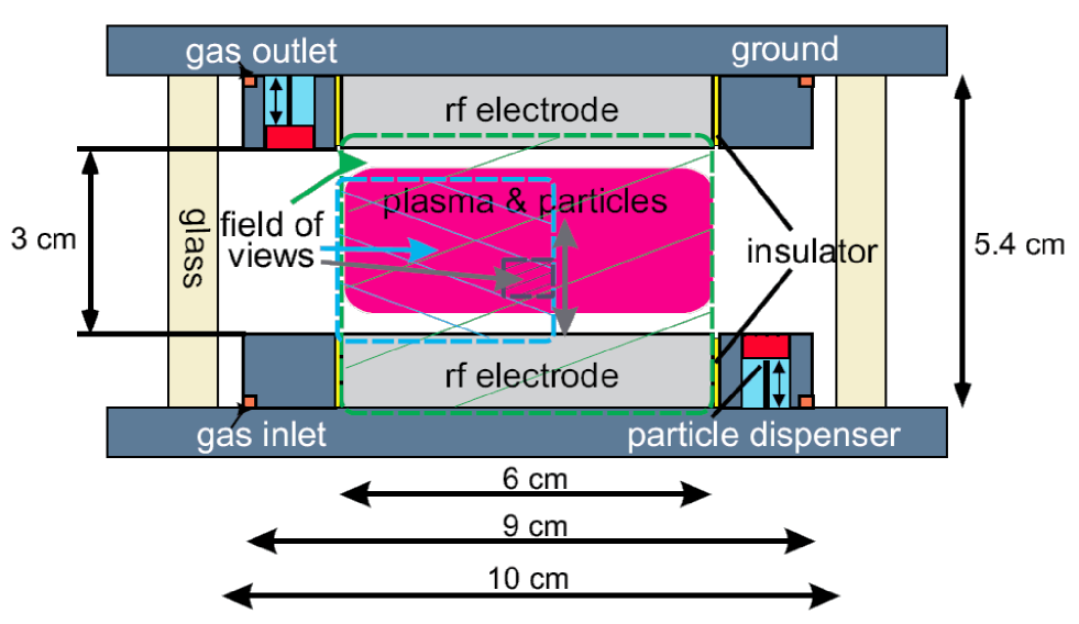
Figure 1:

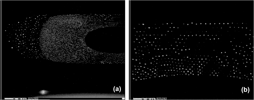
Figure 2:

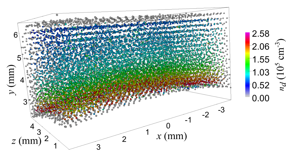
Figure 3:

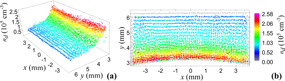
Figure 4:

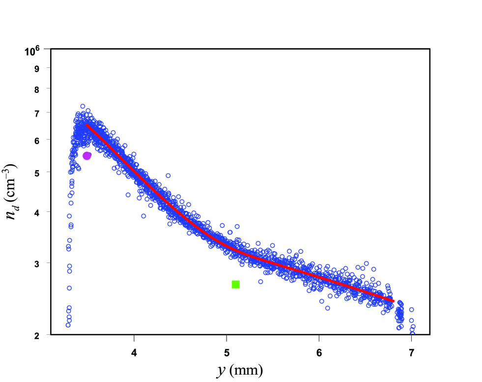
Figure 5:

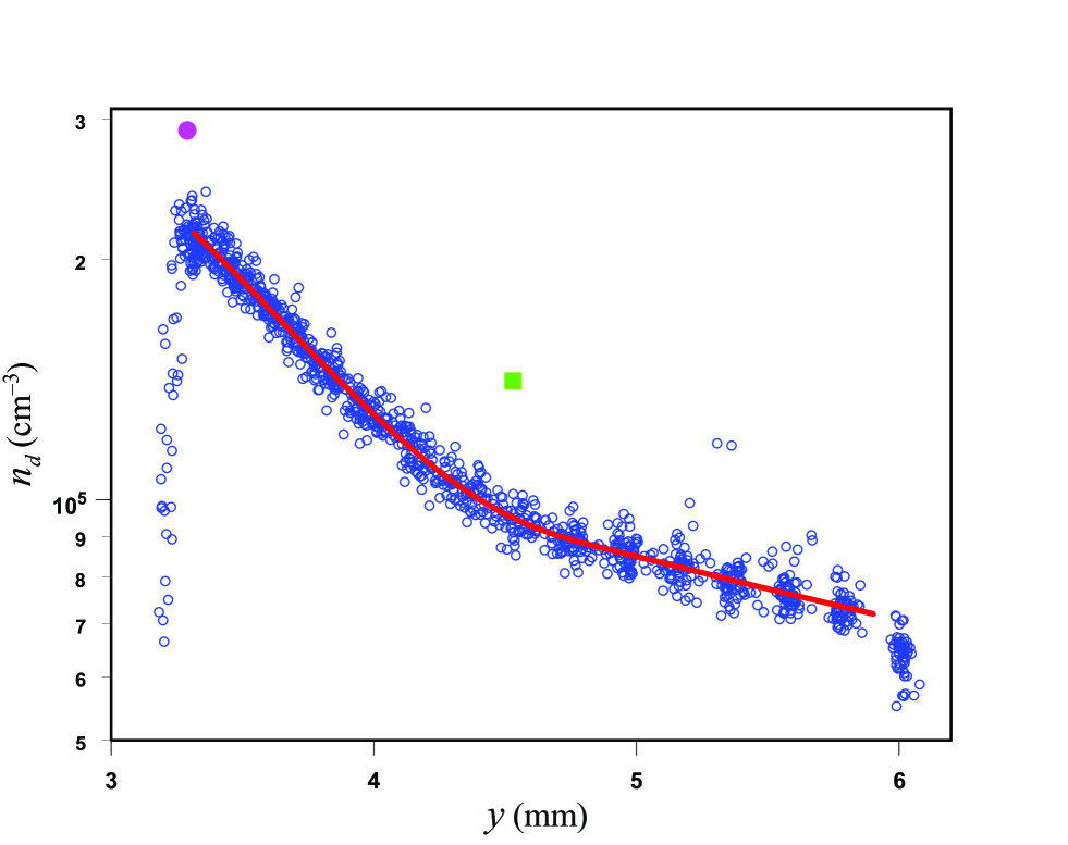
Figure 6:

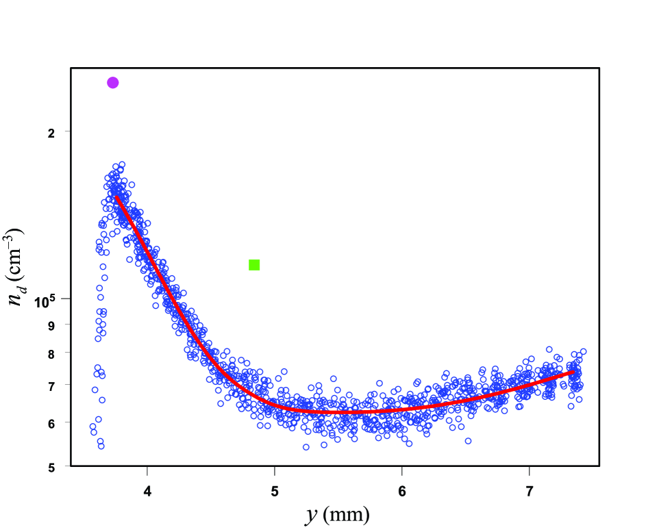
Figure 7:

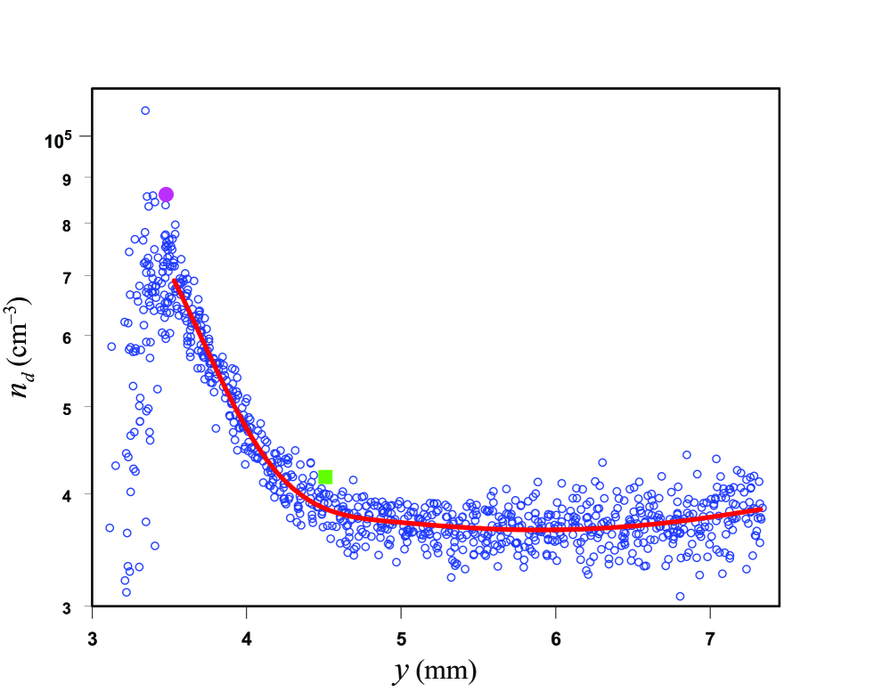
Figure 8:

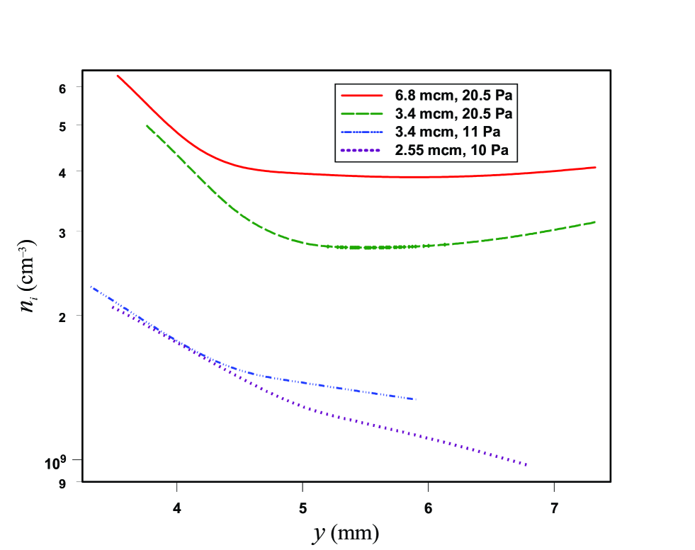
Figure 9:

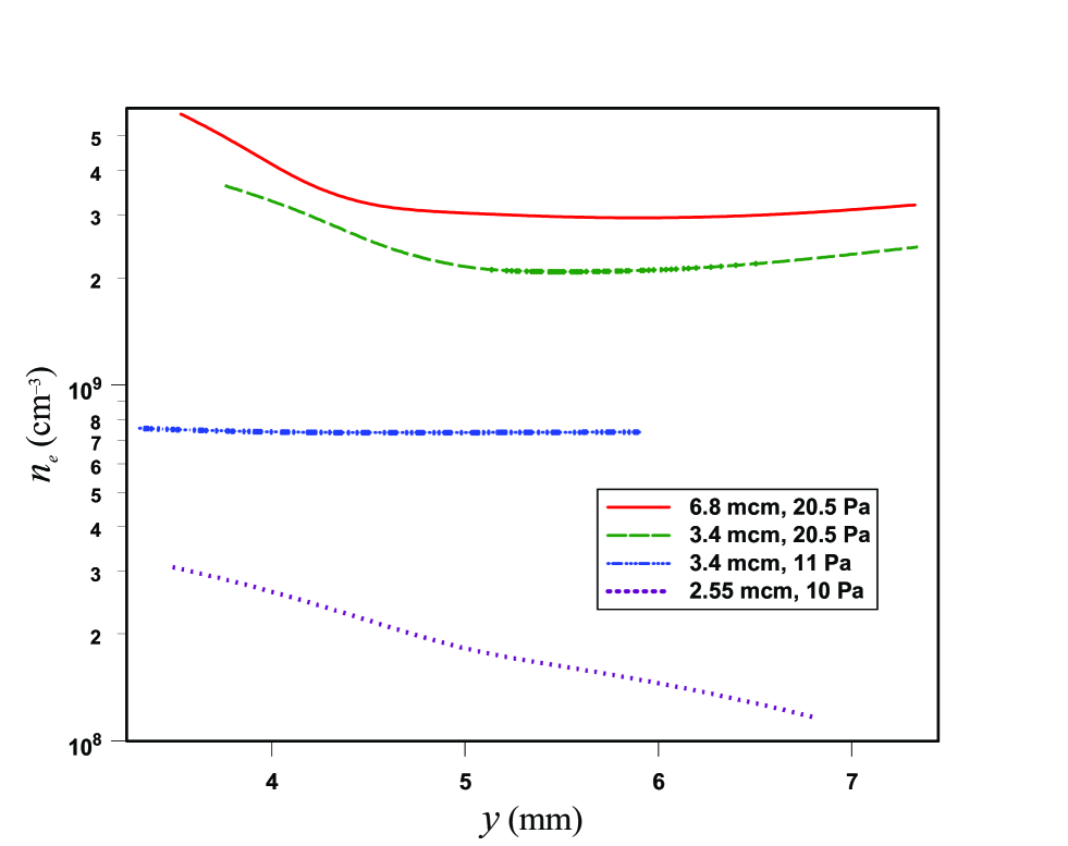
Figure 10:

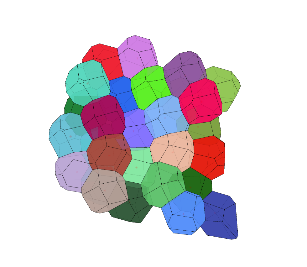
Figure 11:

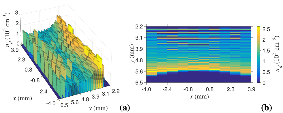
Figure 12:

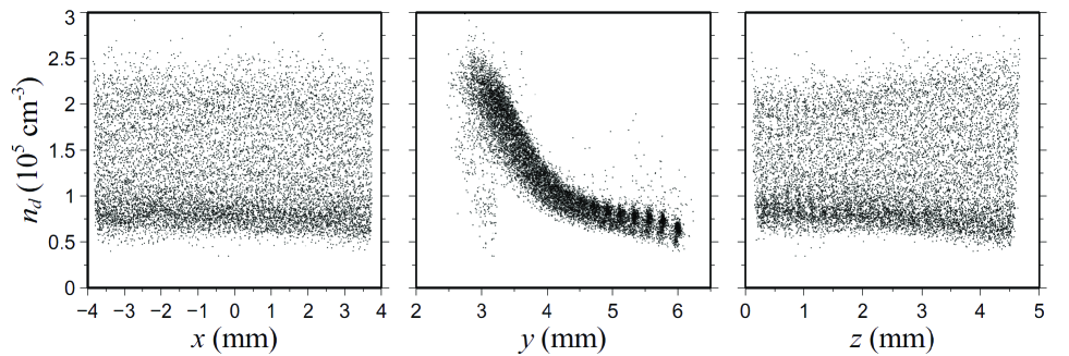
Figure 13:

References

- Fortov and Morfill (2010) V. E. Fortov and G. E. Morfill, eds., Complex and Dusty Plasmas: From Laboratory to Space, Series in Plasma Physics (CRC Press, Boca Raton, FL, 2010).
- Chu and Lin I (1994) J. H. Chu and Lin I, Phys. Rev. Lett. 72, 4009 (1994).
- Thomas et al. (1994) H. Thomas, G. E. Morfill, V. Demmel, J. Goree, B. Feuerbacher, and D. Möhlmann, Phys. Rev. Lett. 73, 652 (1994).
- Vladimirov et al. (2005) S. V. Vladimirov, K. Ostrikov, and A. A. Samarian, Physics and Applications of Complex Plasmas (Imperial College, London, 2005).
- Fortov et al. (2005a) V. Fortov, A. Ivlev, S. Khrapak, A. Khrapak, and G. Morfill, Phys. Rep. 421, 1 (2005a).
- Bonitz et al. (2010) M. Bonitz, C. Henning, and D. Block, Rep. Prog. Phys. 73, 066501 (2010).
- Morfill et al. (2006) G. E. Morfill, U. Konopka, M. Kretschmer, M. Rubin-Zuzic, H. M. Thomas, S. K. Zhdanov, and V. Tsytovich, New J. Phys. 8, 7 (2006).
- Schwabe et al. (2008) M. Schwabe, S. K. Zhdanov, H. M. Thomas, A. V. Ivlev, M. Rubin-Zuzic, G. E. Morfill, V. I. Molotkov, A. M. Lipaev, V. E. Fortov, and T. Reiter, New J. Phys. 10, 033037 (2008).
- Morfill et al. (1999) G. E. Morfill, H. M. Thomas, U. Konopka, H. Rothermel, M. Zuzic, A. Ivlev, and J. Goree, Phys. Rev. Lett. 83, 1598 (1999).
- Khrapak et al. (2011) S. A. Khrapak, B. A. Klumov, P. Huber, V. I. Molotkov, A. M. Lipaev, V. N. Naumkin, H. M. Thomas, A. V. Ivlev, G. E. Morfill, O. F. Petrov, V. E. Fortov, Yu. Malentschenko, and S. Volkov, Phys. Rev. Lett. 106, 205001 (2011).
- Thomas et al. (2008) H. M. Thomas, G. E. Morfill, V. E. Fortov, A. V. Ivlev, V. I. Molotkov, A. M. Lipaev, T. Hagl, H. Rothermel, S. A. Khrapak, R. K. Suetterlin, M. Rubin-Zuzic, O. F. Petrov, V. I. Tokarev, and S. K. Krikalev, New J. Phys. 10, 033036 (2008).
- Jiang et al. (2009) K. Jiang, V. Nosenko, Y. F. Li, M. Schwabe, U. Konopka, A. V. Ivlev, V. E. Fortov, V. I. Molotkov, A. M. Lipaev, O. F. Petrov, M. V. Turin, H. M. Thomas, and G. E. Morfill, Europhys. Lett. 85, 45002 (2009).
- Schwabe et al. (2011) M. Schwabe, K. Jiang, S. Zhdanov, T. Hagl, P. Huber, A. V. Ivlev, A. M. Lipaev, V. I. Molotkov, V. N. Naumkin, K. R. Sütterlin, H. M. Thomas, V. E. Fortov, G. E. Morfill, A. Skvortsov, and S. Volkov, Europhys. Lett. 96, 55001 (2011).
- Khrapak et al. (2012) S. A. Khrapak, B. A. Klumov, P. Huber, V. I. Molotkov, A. M. Lipaev, V. N. Naumkin, A. V. Ivlev, H. M. Thomas, M. Schwabe, G. E. Morfill, O. F. Petrov, V. E. Fortov, Y. Malentschenko, and S. Volkov, Phys. Rev. E 85, 066407 (2012).
- Caliebe et al. (2011) D. Caliebe, O. Arp, and A. Piel, Phys. Plasmas 18, 073702 (2011).
- Klumov (2010) B. A. Klumov, Physics-Uspekhi 53, 1053 (2010).
- Steinhardt et al. (1981) P. J. Steinhardt, D. R. Nelson, and M. Ronchetti, Phys. Rev. Lett. 47, 1297 (1981).
- Aurenhammer (1991) F. Aurenhammer, ACM Computing Surveys 23, 345 (1991).
- Zhukhovitskii et al. (2014) D. I. Zhukhovitskii, V. I. Molotkov, and V. E. Fortov, Phys. Plasmas 21, 063701 (2014).
- Zhukhovitskii (2015) D. I. Zhukhovitskii, Phys. Rev. E 92, 023108 (2015).
- Khrapak et al. (2016) A. G. Khrapak, V. I. Molotkov, A. M. Lipaev, D. I. Zhukhovitskii, V. N. Naumkin, V. E. Fortov, O. F. Petrov, H. M. Thomas, S. A. Khrapak, P. Huber, A. Ivlev, and G. Morfill, Contrib Plasma Phys 56, 253 (2016).
- Nefedov et al. (2003) A. Nefedov, G. Morfill, V. Fortov, H. Thomas, H. Rothermel, T. Hagl, A. Ivlev, M. Zuzic, B. Klumov, A. Lipaev, V. Molotkov, O. Petrov, Y. Gidzenko, S. Krikalev, W. Shepherd, A. Ivanov, M. Roth, H. Binnenbruck, J. Goree, and Y. Semenov, New J Phys 5, 33 (2003).
- Epstein (1924) P. Epstein, Phys. Rev. 23, 710 (1924).
- Khrapak et al. (2002) S. A. Khrapak, A. V. Ivlev, G. E. Morfill, and H. M. Thomas, Phys. Rev. E 66, 046414 (2002).
- Yaroshenko et al. (2005) V. Yaroshenko, S. Ratynskaia, S. Khrapak, M. H. Thoma, M. Kretschmer, H. Höfner, G. E. Morfill, A. Zobnin, A. Usachev, O. Petrov, and V. Fortov, Phys. of Plasmas 12, 093503 (2005).
- Mott-Smith and Langmuir (1926) H. M. Mott-Smith and I. Langmuir, Phys. Rev. 28, 727 (1926).
- Allen (1992) J. E. Allen, Phys. Scr. 45, 497 (1992).
- Zobnin et al. (2000) A. V. Zobnin, A. P. Nefedov, V. A. Sinel’shchikov, and V. E. Fortov, J. Exp. Theor. Phys. 91, 483 (2000).
- Zhukhovitskii et al. (2015) D. I. Zhukhovitskii, V. E. Fortov, V. I. Molotkov, A. M. Lipaev, V. N. Naumkin, H. M. Thomas, A. V. Ivlev, M. Schwabe, and G. E. Morfill, Phys. Plasmas 22, 023701 (2015).
- Fortov et al. (2005b) V. Fortov, G. Morfill, O. Petrov, M. Thoma, A. Usachev, H. Hoefner, A. Zobnin, M. Kretschmer, S. Ratynskaia, M. Fink, K. Tarantik, Yu. Gerasimov, and V. Esenkov, Plasma Phys. Control. Fusion 47, B537 (2005b).
- Nixon and Aguado (2008) M. S. Nixon and A. S. Aguado, Feature Extraction and Image Processing (Academic, New York, 2008) p. 88.