A systematic method to enforce conservativity
on semi-Lagrangian schemes

Abstract

Semi-Lagrangian schemes have proven to be very efficient to model advection problems. However most semi-Lagrangian schemes are not conservative. Here, a systematic method is introduced in order to enforce the conservative property on a semi-Lagrangian advection scheme. This method is shown to generate conservative schemes with the same linear stability range and the same order of accuracy as the initial advection scheme from which they are derived. We used a criterion based on the column-balance property of the schemes to assess their conservativity property. We show that this approach can be used with large CFL numbers and third order schemes.

1 Introduction

Semi-Lagrangian methods have been demonstrated to be efficient schemes to model advection dominated problems. These methods are intensively used to solve atmospheric and weather problems [18, 22], internal geophysics problems [8] or plasma simulations [1, 6, 21]. However, when conservative properties are sought, the method of discretisation usually relies on a finite volume discretisation. Conservativity is then ensured by canceling fluxes, defined on the computational cell boundaries [15, 9].

Semi-Lagrangian methods, on the contrary, are in general not conservative. Some earlier work have tried to address this issue and derive a conservative semi-Lagrangian scheme. For example, [14, 26] introduced a modified version of a non-conservative semi-Lagrangian scheme [23] to enforce conservativity. Their approach provides a conservative formulation at the cost of introducing a scheme in which the coefficients depends on the values of the advected field. An alternative strategy which uses a semi-Lagrangian reconstruction to estimate fluxes on the faces, was introduced by [6] in the finite volume spirit to model the Vlasov equation. This strategy was adapted to compressible flow in [17]. In both of the above approaches, the formulations are well adapted to one-dimensional problems, their generalizations to higher spatial dimensions without using a splitting strategy is challenging.

A general method to enforce conservativity on a semi-Lagrangian scheme was introduced in Lentine et al. [13]. Noting that the contribution of a given cell to the update in time of the total field does not add up to unity, they introduced an ad hoc modification of the coefficients which allows to ensure conservativity at the cost of reducing the order of the scheme.

We propose a systematic method to enforce conservativity on a numerical scheme. Our method, follows ideas introduced in the method of support operators developed by Shashkov [19], or the summation by part method of Carpenter et al. [3, 10]. It can easily be applied to semi-Lagrangian schemes. A close equivalence can be found with the flux interpretation in the sense of finite volume schemes. Let us start by considering the continuity equation, for a quantity $\Phi$ subject to a velocity field $\mathbf{u}$

$$\partial_{t}\Phi=-\mathbf{\nabla}\cdot(\Phi\mathbf{u})\equiv\mathcal{C}(\mathbf{u})[\Phi]\,,$$ (1)

where $\mathcal{C}(\mathbf{u})$ denotes the continuity operator. If the flow is incompressible, $\mathbf{\nabla}\cdot\mathbf{u}=0$, the continuity equation reduces to the advection equation:

$$\partial_{t}\Phi=-\Phi(\mathbf{\nabla}\cdot\mathbf{u})-(\mathbf{u}\cdot\mathbf{\nabla})\Phi=-(\mathbf{u}\cdot\mathbf{\nabla})\Phi\equiv\mathcal{D}(\mathbf{u})[\Phi]\,,$$ (2)

where $\mathcal{D}(\mathbf{u})$ denotes the advection operator.

Instead of considering eq. (2) as a simplified version of eq. (1), under the solenoidal constraint, the two equations can be viewed as two independent equations. Introducing the canonical scalar product of two continuous fields $\Psi$ and $\Phi$, $\left(\Psi\,,\;\Phi\right)=\int\Psi\Phi\mathrm{\;d}\tau\,,$ the continuity and advection operators are then adjoint operator up to a change of the velocity sign:

$$\int\Psi\left[(\mathbf{u}\cdot\mathbf{\nabla})\Phi\right]\mathrm{\;d}\tau=\oint\Psi\Phi\mathbf{u}\cdot\mathbf{n}\mathrm{\;d}s+\int\left[\mathbf{\nabla}\cdot\left(-\mathbf{u}\Psi\right)\right]\Phi\mathrm{\;d}\tau\,.$$ (3)

If the boundary term vanishes, the operators follow: $\left(\Psi\,,\;\mathcal{D}(\mathbf{u})\Phi\right)=\left(\mathcal{C}(-\mathbf{u})\Psi\,,\;\Phi\right)$. Such relations have been intensively used in the support operator formalism [19]. Introducing the $\star$ to denote the adjoint operator, we get: $\mathcal{D}(\mathbf{u})^{\star}=\mathcal{C}(-\mathbf{u})\,.$ This adjoint property can be used to enforce conservativity on an arbitrary advection scheme.

2 Column-balance criterion & Adjoint operator

Using a linear finite difference scheme explicit on time, the advection equation is given by: $\Phi^{n+1}_{i}=\Phi^{n}_{i}+D_{i,j}\Phi^{n}_{j}\,,$, where $D_{i,j}$ denotes the discrete linear operator associated to eq. (2). For the discrete operator to be homogeneous, the coefficients $D_{i,j}$ must only depend on the reduced velocity $U_{i}=u_{i}\Delta t/\Delta x$.

In a similar way, finite difference schemes modeling the continuity equation eq. (1) can be written as $\Phi^{n+1}_{i}=\Phi^{n}_{i}+C_{i,j}\Phi^{n}_{j}$ where $C_{i,j}$ denotes the conservative transport matrix. The evolution of the total mass, $M$, is then given by $M^{n+1}-M^{n}=\sum_{i,j}C_{i,j}\Phi^{n}_{j}=\sum_{i}\Phi^{n}_{i}(\sum_{j}\smash{{}^{\mathrm{t}}\!{C_{i,j}}})\,.$ It follows that the scheme is conservative if and only if the $C_{i,j}$ operator is column-balanced, i.e. for all $i$, $\sum_{j}C_{j,i}=0\,.$ In order to link this formalism to finite volume schemes, the column-balanced conservative matrix can be compared to the flux method. On a regular Cartesian grid, flux are defined at the boundary between two vertices. The equation modeling the flux methods is: $\Phi^{n+1}_{i}=\Phi^{n}_{i}+F_{i-1/2}-F_{i+1/2}\,,$, where $\Phi^{n+1}_{i}$ denotes the values of field $\Phi$ at the index $i$ and $F_{i+1/2}$ the flux of field $\Phi$ computed at index $i+1/2$. Choosing $F_{i+1/2}=C_{i+1,i}\Phi_{i}-C_{i,i+1}\Phi_{i+1}$, both methods are strictly equivalent.

The adjoint relation will now be used to show how a generic advection scheme can be modified to enforce the conservativity property. Once the problem is discrete, the adjoint property leads to: $C(U)=\smash{{}^{\mathrm{t}}\!{D(-U)}}$. It is a property of the transpose that $C(U)$ and $D(-U)$ have the same eigenvalues. Both operators are thus stable for the same set of parameters. They also imply that the error of the $C(U)$ scheme is the transpose of the error of the $D(-U)$ scheme, therefore the two operators have the same consistency order. In addition, if $D(-U)$ is monotone, $C(U)$ is also monotone. Using the Lax-Richtmyer equivalence theorem [12], the consistent and stable $C(U)$ scheme converges to the continuity equation.

The above remarks do not ensure that the $C(U)$ scheme conserves the total mass. However, assuming that the advective scheme is strictly consistent, i.e. $\forall i\,,\;\sum_{j}D_{i,j}(-U)=0$, it follows that $\forall j,\quad\sum_{i}C_{i,j}(U)=0$. The $C_{i,j}(U)$ operator is thus column-balance and conserves the total mass.

It is important to stress that we only introduce a modification of the spatial operator. The conservative property of $C_{i,j}(U)$ will thus be valid both for multi-step and multi-stage time-stepping. Consider for example, a Crank-Nicholson time-stepping scheme [5, 8], the fields at each time steps are related via

$$\left(\delta-\frac{\Delta t}{2}D(U^{n+1})\right)_{i,j}\Phi^{n+1}_{j} =\left(\delta+\frac{\Delta t}{2}D(U^{n})\right)_{i,j}\Phi^{n}_{j}\,,$$ (4)

where $\delta_{i,j}$ denotes the Kronecker delta ($\delta_{i,j}=1$ if $i=j$ and $\delta_{i,j}=0$ if $i\neq j$). The Crank-Nicholson advection operator ($CN$) can be rewritten

$$CN_{i,j}(U) =-\delta_{i,j}+\left[\left(\delta-\frac{\Delta t}{2}D(U^{n+1})\right)^{-1}\left(\delta+\frac{\Delta t}{2}D(U^{n})\right)\right]_{i,j}\,.$$ (5)

The corresponding conservative operator ($CCN$) is then

$$CCN_{i,j}(U) =-\delta_{i,j}+\left[\left(\delta+\frac{\Delta t}{2}\smash{{}^{\mathrm{t}}\!{D}}(-U^{n})\right)\left(\delta-\frac{\Delta t}{2}\smash{{}^{\mathrm{t}}\!{D}}(-U^{n+1})\right)^{-1}\right]_{i,j}\,.$$ (6)

3 Conservative semi-Lagrangian scheme in one dimension

Let us now turn to semi-Lagrangian schemes. The conservative method can be used to generate conservative scheme from a semi-Lagrangian algorithm. In one dimension, the $CIR$ scheme [4], which is equivalent to the upwind scheme, will be used to show how a conservative $CIR$ ($CCIR$) scheme can be built. The resulting $CCIR$ scheme will then be tested on a simple numerical simulation.

In order to be stable, advection algorithm must transport information in the direction of the flow. The $CIR$ scheme satisfies this condition by adapting its stencil according to the direction of the velocity following the characteristic. For advection equation in one dimension (e.g. [24]), the $CIR$ scheme is:

$$\Phi^{n+1}_{i}=\Phi^{n}_{i}+CIR_{i,j}\Phi^{n}_{j}=\Phi^{n}_{i}+(U^{+}_{i}\Phi_{i-1}-|U_{i}|\Phi^{n}_{i}-U^{-}_{i}\Phi^{n}_{i+1})\,,$$ (7)

with $U^{+}_{i}=\max(U_{i},\,0)$ and $U^{-}_{i}=\min(U_{i},\,0).$ To leading order, this scheme yields the diffusive error term

$${[\partial_{t}\Phi+u\partial_{x}(\Phi)]}_{\mbox{\tiny$CIR$}}\!{}\simeq\frac{\Delta x}{2}\,|u|\partial_{x}\left[\left(1-|U|\right)\partial_{x}\Phi\right]\,.$$ (8)

The scheme is consistent with the advection equation, but it is not conservative. The conservative counterpart of the $CIR$ scheme, can be built by changing the sign of the velocity and transposing the $CIR_{i,j}$ matrix. The expression of the $CCIR$ scheme is:

$$\Phi^{n+1}_{i}=\Phi^{n}_{i}+CCIR_{i,j}\Phi^{n}_{j}=\Phi^{n}_{i}+(U^{+}_{i-1}\Phi^{n}_{i-1}-|U_{i}|\Phi^{n}_{i}-U^{-}_{i-1}\Phi^{n}_{i+1})\,.$$ (9)

The $CCIR$ scheme is conservative because it is column-balanced by construction. Similarly to the $CIR$ scheme, the $CCIR$ scheme has a diffusive error. As expected, the $CCIR$ error term is the adjoint of the $CIR$ error term:

$${\left[\partial_{t}\Phi+\partial_{x}(u\Phi)\right]}_{\mbox{\tiny$CCIR$}}\!{}\simeq\frac{\Delta x}{2}\,\partial_{x}\left[\left(1-|U|\right)\partial_{x}(|u|\Phi)\right]\,.$$ (10)

The $CCIR$ scheme was tested using a velocity profile $u(t;x)=\sin(2\pi x)$ and a uniform passive scalar $\Phi(t=0;x)=1$. It conserved the total mass, $M/M_{0}$, near unity up to machine precision. This is not the case of the $CIR$ scheme for varying velocities:

$$\Phi^{n+1}_{i}=\Phi^{n}_{i}+\tfrac{U_{i-1}}{U_{i}}(U^{+}_{i}\Phi^{n}_{i-1})-(|U_{i}|\Phi^{n}_{i-1})+\tfrac{U_{i+1}}{U_{i}}(U^{-}_{i}\Phi^{n}_{i-1})\,.$$ (11)

In the same manner, the second order (dispersive) Lax-Wendroff scheme ($LW$), which takes the form:

$$\Phi^{n+1}_{i}= \left(\tfrac{U^{+}}{U}\tfrac{U(1+U)}{2}\right)_{i}\Phi^{n}_{i-1}+\left(\tfrac{U^{+}}{U}(1-U^{2})\right)_{i}\Phi^{n}_{i}-\left(\tfrac{U^{+}}{U}\tfrac{U(1-U)}{2}\right)_{i}\Phi^{n}_{i+1}$$ (12)

$$+\left(\tfrac{U^{-}}{U}\tfrac{U(1+U)}{2}\right)_{i}\Phi^{n}_{i+1}+\left(\tfrac{U^{-}}{U}(1-U^{2})\right)_{i}\Phi^{n}_{i}-\left(\tfrac{U^{-}}{U}\tfrac{U(1-U)}{2}\right)_{i}\Phi^{n}_{i-1}\,,$$

can be transformed to a conservative $LW$ scheme ($CLW$), of the form,

$$\Phi^{n+1}_{i}= \left(\tfrac{U^{+}}{U}\tfrac{U(1+U)}{2}\Phi^{n}\right)_{i-1}+\left(\tfrac{U^{+}}{U}(1-U^{2})\Phi^{n}\right)_{i}-\left(\tfrac{U^{+}}{U}\tfrac{U(1-U)}{2}\Phi^{n}\right)_{i+1}$$ (13)

$$+\left(\tfrac{U^{-}}{U}\tfrac{U(1+U)}{2}\Phi^{n}\right)_{i+1}+\left(\tfrac{U^{-}}{U}(1-U^{2})\Phi^{n}\right)_{i}-\left(\tfrac{U^{-}}{U}\tfrac{U(1-U)}{2}\Phi^{n}\right)_{i-1}\,.$$

In the same way, the third order (hyperdiffusive) semi-Lagrangian Dahlquist and Björck scheme ($DB$) (e.g. [8, 7]):

$$\Phi^{n+1}_{i}= -\left(\tfrac{U^{+}}{U}\tfrac{U(1-U^{2})}{6}\right)_{i}\Phi^{n}_{i-2}+\left(\tfrac{U^{+}}{U}\tfrac{U(1+U)(2-U)}{2}\right)_{i}\Phi^{n}_{i-1}$$ (14)

$$+\left(\tfrac{U^{+}}{U}\tfrac{(1-U^{2})(2-U)}{2}\right)_{i}\Phi^{n}_{i}-\left(\tfrac{U^{+}}{U}\tfrac{U(1-U)(2-U)}{6}\right)_{i}\Phi^{n}_{i+1}$$

$$-\left(\tfrac{U^{-}}{U}\tfrac{U(1-U^{2})}{6}\right)_{i}\Phi^{n}_{i+2}+\left(\tfrac{U^{-}}{U}\tfrac{U(1+U)(2-U)}{2}\right)_{i}\Phi^{n}_{i+1}$$

$$+\left(\tfrac{U^{-}}{U}\tfrac{(1-U^{2})(2-U)}{2}\right)_{i}\Phi^{n}_{i}-\left(\tfrac{U^{-}}{U}\tfrac{U(1-U)(2-U)}{6}\right)_{i}\Phi^{n}_{i-1}\,,$$

has the following conservative counterpart ($CDB$):

$$\Phi^{n+1}_{i}= -\left(\tfrac{U^{+}}{U}\tfrac{U(1-U^{2})}{6}\Phi^{n}\right)_{i-2}+\left(\tfrac{U^{+}}{U}\tfrac{U(1+U)(2-U)}{2}\Phi^{n}\right)_{i-1}$$ (15)

$$+\left(\tfrac{U^{+}}{U}\tfrac{(1-U^{2})(2-U)}{2}\Phi^{n}\right)_{i}-\left(\tfrac{U^{+}}{U}\tfrac{U(1-U)(2-U)}{6}\Phi^{n}\right)_{i+1}$$

$$-\left(\tfrac{U^{-}}{U}\tfrac{U(1-U^{2})}{6}\Phi^{n}\right)_{i+2}+\left(\tfrac{U^{-}}{U}\tfrac{U(1+U)(2-U)}{2}\Phi^{n}\right)_{i+1}$$

$$+\left(\tfrac{U^{-}}{U}\tfrac{(1-U^{2})(2-U)}{2}\Phi^{n}\right)_{i}-\left(\tfrac{U^{-}}{U}\tfrac{U(1-U)(2-U)}{6}\Phi^{n}\right)_{i-1}\,.$$

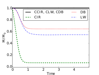
Figure 1: Comparison of the total mass evolution for the $1$D transport problem with $u=\sin(x)$ and $\Phi(t=0)=1$ for conservative and non-conservative semi-Lagrangian schemes of various order (the CFL number is here fixed to $0.75$).

These schemes are compared in figs. 1-3. First, we consider the evolution of the total mass in a simple test case of a periodic flow of the form $u=\sin(x)$ with a constant initial distribution of mass $\Phi(t=0;x)=1$. This is illustrated in fig. 1. The conservative property of the $CCIR$, $CLW$ and $CDB$ schemes is highlighted by the plot of the total mass which remains constant equal to its initial value. Fig. 2 shows standard tests of advection in a periodic domain of a Heaviside, piecewise affine and cosine functions. The diffusive or dispersive behavior generated by the order error term are confirmed. The order can be quantified with more details by considering the error on the amplitude and the phase of the cosine profile (e.g. [2]). Fig. 3 illustrates that the order of the original scheme is maintained for its conservative counterpart.

 (a)

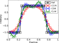
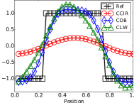
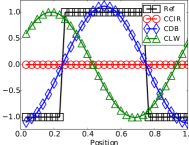
 (b)

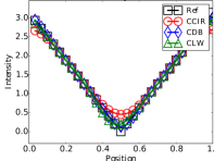
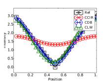
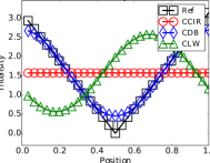
 (c)

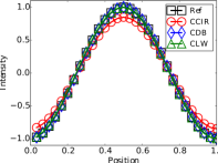
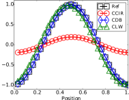
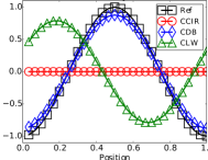
Figure 2: Advection in a periodic domain with periodic boundary conditions. The advection velocity is constant and the initial profile takes the form of a Heaviside (a), a piecewise afine (b), a cosine (c) function. Graphes from left to right correspond to $1$, $10$ and $100$ periods of the flow respectively.

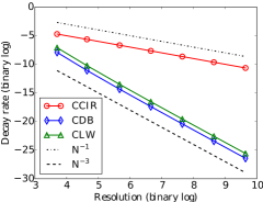
(a) Growth-rate

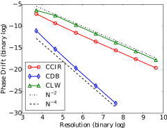
(b) Phase-drift

Figure 3: Decay rate (loss in amplitude) and phase shift per unit of time for the test cases presented in fig. 2 at time $t=5$. The nature of the leading order error term (diffusive or dispersive) is clearly highlighted.

In order to generalize theses scheme to CFL numbers greater than unity, the interpolation point has to be shifted by a integer number of grid spaces, using

$$\tilde{U}_{i}=\left[(u_{i}\Delta t)/\Delta x\right]\%1\;,\;j=i-u_{i}\Delta t/\Delta x+\tilde{U}_{i}\;,\;\tilde{U}^{+}_{i} =\max(\tilde{U}_{i},\,0)\;,\;\tilde{U}^{-}_{i}=\min(\tilde{U}_{i},\,0)\,.$$ (16)

For example, the conservative $CIR$ scheme then becomes

$$\Phi^{n+1}_{i}=\Phi^{n}_{j}+\left[(\tilde{U}^{+}\Phi^{n})_{j-1}-(|\tilde{U}|\Phi^{n})_{j}-(\tilde{U}^{-}\Phi^{n})_{j+1}\right]\,.$$ (17)

Similar expressions follow for the other schemes. The density profiles of the simulation using CFL number above unity, are presented in fig.4 in the case of an initial cosine profile.

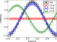
(a) CFL$=0.75$

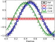
(b) CFL$=2.5$

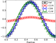
(c) CFL$=7.5$

Figure 4: Advection of a cosine function over $100$ periods of the flow with a CFL number of $0.75$ (a), $2.5$ (b), and $7.5$ (c).

4 Extension in higher dimensions

The standard reconstruction used with the $CIR$ scheme is a bilinear reconstruction. It takes the form:

$$\Phi^{n+1}_{i,j}= [(1-|U|)(1-|V|)\Phi^{n}]_{i,j}[|U|(1-|V|)]_{i,j}\Phi^{n}_{\alpha,j}$$ (18)

$$+[(1-|U|)|V|]_{i,j}\Phi^{n}_{i,\beta}+[|U||V|]_{i,j}\Phi^{n}_{\alpha,\beta}\,,$$

where $V_{i}=v_{i}\Delta t/\Delta x$, $\alpha=i-sign(u_{i,j})$ and $\beta=j-sign(v_{i,j})$.

The above stencil can be interpreted using the geometric construction presented in fig. 5(a). Semi-Lagrangian schemes require to reconstruct the field at the backward advected points ${\bf x}_{i,j}-{\bf u}_{i,j}\Delta t$ . Considering a CFL number smaller than unity, the reconstruction point necessarily lies in one of the cells surrounding ${\bf x}_{i,j}$. This point naturally splits the cell in four parts. The weight of each node in the bilinear interpolation eq. (18) corresponds to the ratio of the surface of the rectangle opposite to this node normalised by to the total surface of the computational cell. This graphical interpretation of eq. (18) is illustrated on fig. 5.a the backward displacement $-{\bf u}_{i,j}\Delta t$ being indicated with a dashed line.

Let us now turn to the conservative scheme, the two-dimensional version of the $CCIR$ scheme can be expressed as:

$$\Phi^{n+1}_{i,j}= [|U^{+}||V^{+}|\Phi^{n}]_{i-1,j-1}+[|U^{+}|(1-|V|)\Phi^{n}]_{i-1,j}+[|U^{+}||V^{-}|\Phi^{n}]_{i-1,j+1}$$

$$+[(1-|U|)|V^{+}|\Phi^{n}]_{i,j-1}+[(1-|U|)(1-|V|)\Phi^{n}]_{i,j}+[(1-|U|)|V^{-}|\Phi^{n}]_{i,j+1}$$ (19)

$$+[|U^{-}||V^{+}|\Phi^{n}]_{i+1,j-1}+[|U^{-}|(1-|V|)\Phi^{n}]_{i+1,j}+[|U^{-}||V^{-}|\Phi^{n}]_{i+1,j+1}\,.$$

It is enlighting to interpret this formula geometrically. The weights now correspond to the forward displacement ${\bf u}_{i,j}\Delta t$, indicated with a solid line on fig. 5.b. Again the weight of each term is given by the relative surface of the rectangle opposite to the advected vertex, normalized by to the total surface of the computational cell. The key distinction is however that the computed weight corresponds to the contribution of $\Phi_{i,j}$ to the time evolution of its neighbors. This contrasts with the $CIR$ scheme, for which the computed weights correspond to the contribution of each neighbor to the evolution of $\Phi_{i,j}$.

In fig. 5, mass conservation appears as a direct consequence of the fact that the sum of each sub-rectangle amounts to the total cell as highlighted by expression (19). Let us stress that this approach results in a conservative non-split semi-Lagrangian formulation.

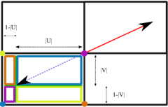
(a) Advection sketch

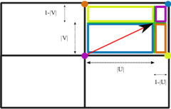
(b) Continuity sketch

Figure 5: Illustration of the reconstruction strategy and computational weights for the standard $CIR$ scheme (a) and its conservative $CCIR$ counterpart (b). The red arrow corresponds to the forward advection. The color of a rectangle, indicates its contribution in the evolution of a given point with the same color (see text).

A few observations can be made on this stencil. First, this rather simple geometric interpretation can be generalized to higher dimensions. Second, the two-dimensional $CCIR$ stencil of eq. (19) is identical to the split formula corresponding to the composition of two one-dimensional $CCIR$ stencils, $CCIR_{xy}=CCIR_{x}\circ CCIR_{y}=CCIR_{y}\circ CCIR_{x}$. Such is not the case for the $CIR$ stencil. This commuting property can be used to generalize the higher-order conservative schemes from section 3 to higher dimensions of space.

To illustrate the conservative property of the $CCIR$ scheme in two dimensions of space, it was tested using an incompressible velocity profile of the form $u(t;x,y)=-\sin(\pi x)\cos(2\pi y)$, $v(t;x,y)=\cos(\pi x)\sin(2\pi y)$. The initial passive scalar field takes the form of a uniform patch $\Phi(t=0;x,y)=1$ if $|x-0.5|\leq 0.15$ and $|y-0.3|\leq 0.15\,,$ and $0$ elsewhere (see fig. 6.a).

Since the flow is incompressible, the advection and continuity equation are equivalent. We thus compare the three schemes discussed in section 3 and their conservative counterpart. In fig. 6b, the evolution of relative total mass of the $CIR$, $LW$ and $DB$ schemes is represented. As expected, the conservative schemes have a relative mass equal to unity, up to machine precision for the same set of parameters.

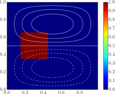
(a) Initial density profile

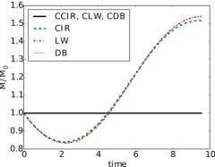
(b) Mass evolution with time.

Figure 6: Two dimensional transport of a density distribution initially uniform within a square (a). The total mass evolution with time up to $t=10$ with a resolution of $128^{3}$ for conservative and non-conservative semi-Lagrangian schemes of first, second and third order (b) reflects the conservative nature of the schemes.

In fig. 7, color-plots of the density profile are given for all schemes at $t=10$. The evolution of mass in the plan of symmetry is different for all schemes. The accumulation of mass near the stagnation point is clearly visible with the conservative schemes of odd orders, see figs. 7(d) and 7(f). Dispersive effects in fig. 7(e), which do not vanish in the symmetry plane, are still too strong to allow for this feature to emerge.

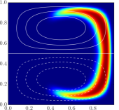
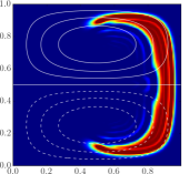
 (a)  (b)  (c)

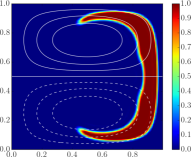
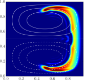
 (d)  (e)  (f)

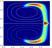
 (g)  (h)  (i)

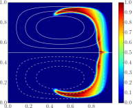
Figure 7: A comparison of the non-conservative scheme at CFL$=0.8$ (a,b,c) with the conservative scheme at CFL$=0.8$ (d,e,f) and at CFL$=1.6$ (g,h,i). The simulation were carried out at a resolution of $128^{2}$ for an integration time of $t=10$.

The explicit scheme introduced in eq. (19) corresponds to a first order time integration. We should stress however that the modified reconstruction strategy introduced to enforced conservativity only concerns the spatial operator. The conservative property is thus retrained for higher order or multi-level time-stepping algorithms as shown in eqs.(5) and (6).

In fig. 8, convergence effects can clearly be identified by comparing results obtained with the $CCIR$ scheme (conservative, first order) with a fine grid ($1024^{2}$), to the ones obtained with a coarser grid ($128^{2}$) or with the $CDB$ scheme (conservative, third order). At low resolution, owing to the effects of the numerical diffusion, the density on fig. 8(a) appears to be spread across three independent lobes. Increasing the resolution, or using a higher-order scheme, reveals the fine filaments of mass connecting these lobes.

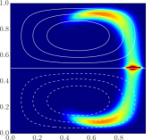
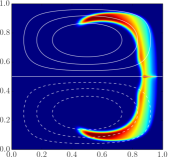
 (a)  (b)  (c)

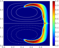
Figure 8: Comparison of the first order conservative $CCIR$ scheme with the third order conservative $CDB$ scheme at CFL$=0.8$. Plots (a) and (b) compare simulations of resolution $128^{2}$ and $1024^{2}$ respectively for the $CCIR$ scheme; plot (c) presents the same setup solved with the $CDB$ scheme at a resolution of $128^{2}$.

Varying the resolution, the convergence of the density profile is tested for the conservative diffusive monotone $CCIR$ scheme at CFL$=1.6$ in fig. 9. As the resolution increases at constant CFL, the numeric error decreases and the density profile becomes closer to the analytic solution. At high resolution, the grid is finer, the simulation is therefore more precise and catches the details of the structure near the symmetry axis.

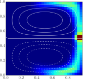
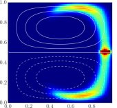
 (a)  (b)  (c)

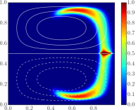
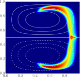
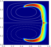
 (d)  (e)  (f)

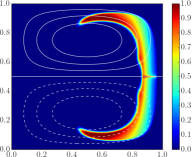
Figure 9: Convergence study for the first order conservative $CCIR$ at CFL$=1.6$ with resolutions: $(a):32^{2}\,,\ (b):64^{2}\,,\ (c):128^{2}\,,\ (d):256^{2}\,,\ (e):512^{2}\,,\ (f):1024^{2}\,.$

At a resolution of $256^{2}$, the $CCIR$ is able to got accurately the profile for CFL number above unity. Fig. 10 shows the profile computed for CFL up to $8$. Comparing the profiles on figs. 9 and 10 with the profile of the $1024^{2}$ resolution simulation at CFL$=0.8$ of fig. 8(b), the conservative schemes are able to model the flow for CFL$>1$ with great accuracy. The excellent agreement between the simulation is not restricted to the profile, it also extent to the total mass which is conserved up to machine precision.

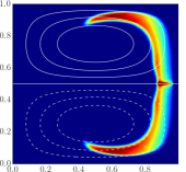
 (a)  (b)  (c)

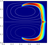
Figure 10: Comparison the profile of simulations using the first order $CCIR$ scheme at a resolution of $256^{2}$ for different CFL: $(a):1.6\,,(b):4.0\,,(c):8.0$.

Semi-Lagrangian algorithms are composed of two main steps [16, 20, 6]: the computation of the characteristic curves, and the reconstruction step. The present work was centered on making the reconstruction step conservative. All the simulation carried out used the $2D$-generalization of eq. (16). Even though the trajectories were computed with a law order method, the algorithm can be adapted to more sophisticated methods. To do so, the trajectory in each point can be reconstructed using high order characteristics (e.g. [6]) and the resulting displacement should be decomposed as the sum of : (i) a vector whose components are equal to an integer number of grid-steps, and (ii) a remainder vector whose components are smaller than the grid-step.

5 Perspectives

We have introduced a systematic approach to derive a conservative scheme without the need for a finite volume discretisation. The method has been successfully applied to semi-Lagrangian schemes, which are notorious for being very efficient, but usually not conservative. Using this method, we were able to built a third order conservative semi-Lagrangian scheme based on the scheme introduced by Dahlquist and Björck.

The approach presented here is similar in the spirit to that introduced by Verstappen et al. in [25] to derive energy preserving schemes. They also used an adjoint formulation to derive the discrete scheme. As their concern is the conservation of energy, they insist of the skew symmetry property of the operator. We are here rather concerned with mass conservation and therefore focus on the column-balance property of the scheme.

Our approach also bears similarities with ideas introduced by Shashkov in the support operators method [19] or by Carpenter [3, 10]. It however differs from the support operator method, in that we propose an algorithm (via the discretisation of the adjoint equation) to systematically transform a non-conservative advection scheme into a continuity preserving operator.

Appendix A Convergence study

In order to illustrate the order of convergence of the conservative schemes introduced in section 3 in $2$D, we perform a numerical study with varying resolution. The initial distribution takes the form $\cos(x+y)$ and the flow is uniform with $u_{x}=u_{y}=1$. The results are illustrated in fig. 11 and in tables 1 and 2.

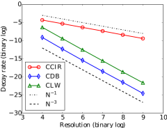
(a) Growth-rate

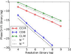
(b) Phase-drift

Figure 11: Decay rate (loss in amplitude) and phase shift per unit of time for a 2D test case, the initial distribution takes the form $\cos(x+y)$ and the flow is uniform with $u_{x}=u_{y}=1$.

Resolution	CCIR	CLW	CDB
16	0.050728	0.012718	0.0018352
32	0.025286	0.0014777	0.00019944
64	0.012492	0.00017356	2.3e-05
128	0.0061982	2.1e-05	2.8e-06
256	0.0030018	2.51e-06	3.49e-07
512	0.0014981	3.19e-07	4.16e-08

Table 1: Decay rate for the 2D advection test.

Resolution	CCIR	CLW	CDB
16	0.0047106	0.028943	0.00020718
32	0.0010636	0.0072473	1.0516e-05
64	0.00025402	0.0017658	5.4912e-07
128	6.2017e-05	0.00043328	4.4307e-08
256	1.6382e-05	0.0001072	2.3758e-09

Table 2: Phase shift for the 2D advection test.

References

- [1] N. Besse and E. Sonnendrucker, Semi-Lagrangian schemes for the Vlasov equation on an unstructured mesh of phase space, Journal of Computational Physics, 191 (2003), pp. 341–376.
- [2] A. Cameron, R. Raynaud, and E. Dormy, Multi-stage high order semi-Lagrangian schemes for incompressible flows in Cartesian geometries, International Journal for Numerical Methods in Fluids, (2016).
- [3] M. H. Carpenter, J. Nordström, and D. Gottlieb, A Stable and Conservative Interface Treatment of Arbitrary Spatial Accuracy, Journal of Computational Physics, 148 (1999), pp. 341–365.
- [4] R. Courant, E. Isaacson, and M. Rees, On the solution of nonlinear hyperbolic differential equations by finite differences, Comm. Pure Appl. Math., 5 (1952), pp. 243–255.
- [5] J. Crank and P. Nicolson, A practical method for numerical evaluation of solutions of partial differential equations of the heat-conduction type, Mathematical Proceedings of the Cambridge Philosophical Society, 43 (1947), pp. 50–67.
- [6] Nicolas Crouseilles, Michel Mehrenberger, and Eric Sonnendrücker, Conservative semi-Lagrangian schemes for Vlasov equations, Journal of Computational Physics, 229 (2010), pp. 1927–1953.
- [7] G. Dahlquist and A. Bjorck, Numerical Methods, Prentice Hall, Englewood Cliffs, New York, (1974).
- [8] D. R. Durran, Numerical methods for wave equations in geophysical fluid dynamics, no. 32, Springer, 1999.
- [9] R. Eymard, T. Gallouët, and R. Herbin, Finite volume methods, in Handbook of Numerical Analysis, P. G. Ciarlet and J. L. Lions, ed., vol. 7 of Solution of Equation in R^n (Part 3), Techniques of Scientific Computing (Part 3), Elsevier, 2000, pp. 713–1018.
- [10] T. C. Fisher, M. H. Carpenter, J. Nordström, N. K. Yamaleev, and C. Swanson, Discretely conservative finite-difference formulations for nonlinear conservation laws in split form: Theory and boundary conditions, Journal of Computational Physics, 234 (2013), pp. 353–375.
- [11] K. O. Friedrichs and P. D. Lax, Systems of Conservation Equations with a Convex Extension, Proceedings of the National Academy of Sciences, 68 (1971), pp. 1686–1688.
- [12] P. D. Lax and R. D. Richtmyer, Survey of the stability of linear finite difference equations, Communications on Pure and Applied Mathematics, 9 (1956), pp. 267–293.
- [13] M. Lentine, J.T. Grétarsson, and R. Fedkiw, An unconditionally stable fully conservative semi-Lagrangian method, Journal of computational physics, 230 (2011), pp. 2857–2879.
- [14] T. Nakamura, R. Tanaka, T. Yabe, and K. Takizawa, Exactly Conservative Semi-Lagrangian Scheme for Multi-dimensional Hyperbolic Equations with Directional Splitting Technique, Journal of Computational Physics, 174 (2001), pp. 171–207.
- [15] S. V. Patankar, Numerical Heat Transfer and Fluid Flow, CRC Press, Jan. 1980.
- [16] J. Pudykiewicz and A. Staniforth, Some properties and comparative performance of the semi‐Lagrangian method of Robert in the solution of the advection‐diffusion equation, Atmosphere-Ocean, 22 (1984), pp. 283–308.
- [17] J.-M. Qiu and C.-W. Shu, Conservative high order semi-Lagrangian finite difference WENO methods for advection in incompressible flow, Journal of Computational Physics, 230 (2011), pp. 863–889.
- [18] A. Robert, A stable numerical integration scheme for the primitive meteorological equations, Atmosphere-Ocean, 19 (1981), pp. 35–46.
- [19] M. Shashkov, Conservative Finite-Difference Methods on General Grids, CRC Press, Dec. 1995.
- [20] Piotr K. Smolarkiewicz and Janusz A. Pudykiewicz, A Class of Semi-Lagrangian Approximations for Fluids, Journal of the Atmospheric Sciences, 49 (1992), pp. 2082–2096.
- [21] E. Sonnendrucker, J. Roche, P. Bertrand, and A. Ghizzo, The Semi-Lagrangian Method for the Numerical Resolution of the Vlasov Equation, Journal of Computational Physics, 149 (1999), pp. 201–220.
- [22] A. Staniforth and J. Côté, Semi-Lagrangian Integration Schemes for Atmospheric Models—A Review, Mon. Wea. Rev., 119 (1991), pp. 2206–2223.
- [23] H. Takewaki, A. Nishiguchi, and T. Yabe, Cubic interpolated pseudo-particle method (CIP) for solving hyperbolic-type equations, Journal of Computational Physics, 61 (1985), pp. 261–268.
- [24] E. F. Toro, Riemann Solvers and Numerical Methods for Fluid Dynamics, Springer Berlin Heidelberg, Berlin, Heidelberg, 2009.
- [25] R. W. C. P. Verstappen and A. E. P. Veldman, Symmetry-preserving discretization of turbulent flow, Journal of Computational Physics, 187 (2003), pp. 343–368.
- [26] F. Xiao and T. Yabe, Completely Conservative and Oscillationless Semi-Lagrangian Schemes for Advection Transportation, Journal of Computational Physics, 170 (2001), pp. 498–522.