Neutral Hydrogen and its Emission Lines in the Solar Corona

1 Introduction

It came as a surprise to discover that a hot and diluted medium such as the corona was emitting the “cool” L$\alpha$ line (Gabriel, 1971). Since this rocket observation (eclipse), many more L$\alpha$ observations have been performed (e.g. Hassler et al. (1994) and Kohl et al. (1995) by the Ultraviolet Coronal Spectrometer (UVCS) on board Spartan, and later on by the Ultraviolet Coronal Spectrometer (UVCS) on board the Solar and Heliospheric Observatory (SOHO) (Zangrilli et al. (1999) and Maccari et al. (1999))) with the help of a coronagraph. The emission was quickly identified as the resonance scattering of the chromospheric L$\alpha$ radiation by “trace” neutral hydrogen (usually taken as about $10^{-6}$ electron density). Because L$\alpha$ is the strong resonance line of the most abundant element (hydrogen) and because the emitted chromospheric profile is about as wide as the absorption profile of coronal neutral hydrogen, in the absence of velocity field, the emission is rather strong (about $10^{-6}$ the disk value at 1.5 R_⊙) and even stronger (a few $10^{-5}$) in a streamer (e.g. Miralles et al., 1999). This is why a major future mission, Solar Orbiter, includes the L$\alpha$ coronograph called Multi Element Telescope for Imaging and Spectroscopy (METIS) (Antonucci et al., 2012). Moreover, it has been shown as early as 1982 (Bommier and Sahal-Brechot, 1982) that the line was sensitive to the Hanle effect (generally effective in weak magnetic fields). Consequently, many (space) projects have proposed polarimetric measurements in this line (e.g. the Small Explorer for Solar Eruptions (SMESE) mission (Vial et al., 2007) and more recently the Coronal UV spectro-polarimeter (CUSP) on board the Solar magnetism eXplorer (SolmeX) (Peter et al., 2012), the MAGnetic Imaging Coronagraph (MAGIC) on board the INvestigation of Solar-Terrestrial Activity aNd Transients (INSTANT) mission (Lavraud et al. (2015), proposal to ESA), the MAGnetic Imaging Coronagraph (MAGIC) on board the Magnetic Activity of the Solar Corona (MASC) mission (Auchère et al. (2015), proposal to ESA). It has also been proposed to use the L$\beta$ line for performing polarimetric measurements in the faint corona (Peter et al., 2012).
However, until now, these projects are still at the proposal level for various reasons including the (relative) complexity of the instrumentation and the fact that polarimetry is “photon-hungry” and requires large apertures in the ultra-violet (UV). Apart from radio observations above active regions, another path towards coronal polarimetry has been pursued with ground-based infrared (IR) observations measuring the Zeeman effect (Lin, Penn, and Tomczyk, 2000; Tomczyk et al., 2008).
Another possibility has been opened with eclipse polarization measurements in red and green channels by Kim et al. (2013b) from which these authors concluded that “the polarization excess (green-red) can be explained by the presence of neutral hydrogen in the corona” (see also Dolei et al., 2014). As mentioned by Kim et al. (2013b), Poland and Munro (1976) and Mierla et al. (2011) had already concluded that H$\alpha$ contributed to coronagraphic images of transients and coronal mass ejections (CMEs), respectively. Actually this was demonstrated with eclipse measurements made at the Canada-France-Hawaï Telescope (CFHT) in 1991 where Vial et al. (1992) detected a plasmoid in the solar corona that Koutchmy et al. (1994) interpreted as emitting essentially in the H$\alpha$ line, a claim discussed later on by Zhukov et al. (2000) who proposed an upper limit of the emission of about 2 % of the background corona. Moreover, the Hanle effect has been successfully used in the H$\alpha$ line, in spite of its optical thickness, in magnetic-field measurements in prominences (e.g. Leroy, 1981; Bommier, Sahal-Brechot, and Leroy, 1981).
In order to derive the plasma properties (including magnetic field) it is imperative to take into account all processes involved and first of all the proper ionization degree. The aim of this work is to compute most observable parameters (line profile, intensity) for the main H lines exactly emitted by (three) typical regions of the solar corona and at various heights above the limb.
In Section section2, we present the full non-LTE computations derived from 1D non-LTE codes which are adapted to the geometry of the corona. In Section section3, we focus on profiles obtained in the L$\alpha$, L$\beta$ and H$\alpha$ lines at various heights. In Section comparaison_Ly_obs, we also compare with other computational and observational results in the L$\alpha$ and L$\beta$ lines. In Section section4, we provide the variation with altitude of the ionization degree for the three models. In Section section5, we discuss all our results, and we pay some attention to the possibility of observing the H$\alpha$ line in the corona. In Section section6, we conclude on further improvements in the computations.
We also present in the Appendix an approximation to obtain the H$\alpha$ intensity from the (measured) L$\alpha$ emission.

2 Non-LTE Computations

section2 As far as hydrogen lines are concerned, we remark that the radiative output of structures such as prominences and the corona is dominated by the incident radiation and the resonance scattering that follows. The L$\alpha$ case has been extensively studied since the pioneering work of Heasley and Mihalas (1976) who built a non-LTE code adapted to one dimensional cool layers located in the corona illuminated by the photospheric, chromospheric and coronal radiation. Much modeling has been performed since (e.g. Gouttebroze, Heinzel, and Vial, 1993) where the prominence was considered as an isothermal and isobaric layer. More recently, prominence–corona transition regions (PCTR) have been grafted to the homogeneous layer on the basis of magnetohydrostatic (mhs) equilibrium by Anzer and Heinzel (1999) and then consistent mhs models of threads have been combined with the addition of inhomogeneous layers (Heinzel, Anzer, and Gunár, 2005); for comprehensive reviews of this modeling, see Labrosse et al. (2010), Gunár (2014), Labrosse (2015) and Heinzel (2015). In all these recent models, there is basically a cool core (T $\approx$ 10 000 K) and a PCTR where physical quantities vary drastically up to the corona itself where the density is low enough for all the lines and continua of all elements (including hydrogen) to be optically thin. In the low corona, the Lyman lines have been treated by Noci, Kohl, and Withbroe (1987) with the simple assumption of resonance scattering to begin with and later on with the inclusion of electron collisions, which allows for more information to be drawn from L$\alpha$ and L$\beta$ observations (Withbroe et al., 1982; Raymond et al., 1997). As shown by Labrosse, Li, and Li (2006) in the case of a coronal streamer, the L$\alpha$ line is essentially radiatively formed but the L$\beta$ line becomes increasingly collisionnally driven with increasing altitude. Moreover, as discussed in Section section4, the ionization has been computed up to now within the simplified model of Gabriel (1971).
For various reasons (including its non-detection even with the best coronagraphs, the best seeing, and the most narrow filters), the coronal H$\alpha$ line has never been studied in detail. It is formed in the corona through various processes (radiative and partly collisional) involving at least the three first levels and possible cascades from higher levels including the continuum. In the Appendix, we propose a simple approach for computing H$\alpha$, an approach which involves radiative processes and the first three levels only.
In order to perform an exact computation of the hydrogen lines (which implies to compute a high number of population levels, including the continuum, with all processes taken into account), we decided to follow a “non-LTE radiative transfer” approach although it is clear that because of the low neutral density in the corona (about $10^{-6}$ times the electron density) all hydrogen lines are optically thin and all resonance scatterings are not followed by a second scattering. The advantage is that the bulk of the code is available and well controlled, in such a way that it is then possible to treat many hydrogen levels (including the continuum) with precise incident radiation altitude-dependent profiles which are critical for the population of H levels. This approach does not simplify the incident profiles, contrary to Auchère (2005) or Dolei, Spadaro, and Ventura (2015), who use a combination of three gaussians. It formally allows for the consideration of incident profiles varying with distance to the limb, or with the presence of close active regions, or the variation with activity. As far as the thermodynamic parameters, density [$n_{e}$] and temperature [$T_{e}$] of the corona are concerned, they vary with radial distance (see Section sect_2.2). As already mentioned, such an approach has been followed by Labrosse, Li, and Li (2006) who computed the L$\alpha$ and L$\beta$ integrated intensities in a streamer defined through the three-fluid solar-wind model of Li, Li, and Labrosse (2006). However, we proceeded with a different method and different models as shown below.

2.1 The Computational Method

The initial prominence code, PROM5 (https://idoc.ias.u-psud.fr/
MEDOC/Radiative transfer codes/PROM5) is modified as follows. Instead of a cool core with an extended PCTR, we simply have no layer with low temperature but only a so-called PCTR with actual coronal conditions in a spherically symmetric configuration where the density decreases from the impact parameter position toward both sides of the line-of-sight (LOS). The medium being optically thin in all lines and in all directions, the incident radiation is exactly computed at each radial distance. Actually, the computation of the L$\alpha$ line emitted when the line-of-sight crosses the limb (and where a plane-parallel LOS computation makes no sense) has been performed in the more difficult case of an optically thick atmosphere (Vial, 1970). In order to simplify the computations, we adopted the same model extension, for all LOS located at altitudes between 1.05 and 5 R_⊙. This means that the boundaries along each LOS are (symmetrically) defined by the last external layer of the radial model. Through extrapolation, we checked that the neglected (out-of-model) parts along the LOS did not contribute much to the computed opacities (i.e. intensities): for L$\alpha$ we found less that 1 % at 1.05 R_⊙ and much less for the other lines and lower altitudes. For higher altitudes (i.e. 5 R_⊙), the neglected opacity reaches 4 % for the coronal hole model.
The dedicated coronal code, PROMCOR is available at:
https://idoc.ias.u-psud.fr/MEDOC/Radiative transfer codes/PROMCOR
where a typical coronal hole model is proposed as an input.

2.2 The Physical Models

sect_2.2 We limited our study to three different models: the quiet corona and polar coronal hole models provided by Allen (1977) and the streamer model of Goryaev et al. (2014). The streamer model is provided in 2D as an angular diverging slab with a Gaussian shape with a constant temperature of $1.43\times 10^{6}$ K as derived from the measurements from the Sun Watcher using Active Pixel System Detector and Image Processing (SWAP) and the EUV imaging spectrometer (EIS) on board Hinode. We simplified the model into a spherically symmetric one with a temperature of $10^{6}$ K in order to better compare with the quiet corona values of Allen (1977). Note that Dolei, Spadaro, and Ventura (2015) found a temperature range of $5\times 10^{5}$ K – $1.5\times 10^{6}$ K between 2 and 6 R_⊙, over a large range of position angles. We adopted the radial density provided by Equation (16) and Table 2 of Goryaev et al. (2014). In doing so, we do not have to take into account any background contribution since we have a unique geometrical model but we are aware that all our LOS intensities are overestimated as compared to the actual Goryaev model. In order to roughly compare the L$\alpha$ and L$\beta$ results with the streamer model we selected two lines of sight: one at 1.05 R_⊙ and the other at 1.9 R_⊙.
The initial density profile of the three models (quiet Sun, coronal hole, and streamer) along the two halfs of the LOS is shown in Figure fig1.
We can note that our streamer electron density (half) profiles along the LOS have roughly the same magnitudes and shapes as the streamer profile of Labrosse, Li, and Li (2006).
As far as the temperature profile is concerned, as mentioned above, we used the temperature variation with altitude of Allen (1977) for the quiet Sun; we took a constant temperature of 800,000 K (see David et al., 1998) for the coronal hole and, as mentioned above, kept a constant temperature of $10^{6}$ K for the streamer model (see Goryaev et al., 2014).

Figure 1.: Electron densities for the quiet Sun, coronal hole, and streamer models at two altitudes: 1.05 and 1.9 R_⊙, along half of the LOS.fig1

3 Computed Profiles and Variation of the Integrated Intensities with the Altitude of the LOS

section3 Since we assume no velocity field (neither radial nor along the LOS), we only compute half-profiles which are shown in Figures fig2 (L$\alpha$), fig3 (L$\beta$), and fig4 (H$\alpha$). Note that we limit ourselves to the presentation of the three lines but more lines have been computed since we have a five-level atom.
It is important to stress that the H$\alpha$ (half) profiles in Figure fig4 have been computed without any continuum absorption. This allows to compare the integrated intensities in the three main lines on one hand (Figures fig5-1 and fig5-2) and, as far as the streamer is concerned, to compare with the L$\alpha$, L$\beta$ results of Labrosse, Li, and Li (2006), on the other hand. However, as shown in this section, the inclusion of absorption is critical for the H$\alpha$ line.
First, we note that for all models (Figures fig5-1 and fig5-2) the L$\beta$ intensity is an order of magnitude smaller than the L$\alpha$ intensity at $r=1.05~{}R_{\odot}$, leading to a ratio (0.07) which is higher than the ratio of the incident intensities (between 0.011 and 0.014 according to Lemaire et al. (2012)). This ratio becomes $1.3\times 10^{-2}$ at 1.9 R_⊙, a value equal to the ratio of the incident intensities and to be compared with the $2\times 10^{-3}$ observed value of Ciaravella et al. (2003) at a distance of 2.3 R_⊙ in a pre-CME streamer (and a value slightly higher in the CME, or its “prominence core”, as stated by these authors). This can be interpreted as the result of the large (average) densities in our one-dimensional streamer model, which increase the collisional component of the L$\beta$ intensity and the excitation of level 3 through 1–2 and 2–3 absorption and spontaneous emission from level 3 to level 1.

Figure 2.: Half-profiles of the L$\alpha$ line for LOS at 1.05 (first row, (a) and (b)) and at 1.9 R_⊙ (second row, (c) and (d)).
On the left column ((a) and (c)) the half-profiles for the quiet-Sun and coronal-hole models.
On the right column ((b) and (d)) the half-profiles for the streamer model.fig2

Figure 3.: Half-profiles of the L$\beta$ line for LOS at 1.05 (first row, (a) and (b)) and at 1.9 R_⊙ (second row, (c) and (d)).
On the left column ((a) and (c)) the half-profiles for the quiet-Sun and coronal-hole models.
On the right column ((b) and (d)) the half-profiles for the streamer model.fig3

Figure 4.: Half-profiles of the H$\alpha$ line for LOS at 1.05 (first row, (a) and (b)) and at 1.9 R_⊙ (second row, (c) and (d)).
On the left column ((a) and (c)) the half-profiles for the quiet-Sun and coronal-hole models.
On the right column ((b) and (d)) the half-profiles for the streamer model.fig4

Second, another interesting feature is the ratio between the L$\beta$ and H$\alpha$ integrated intensities which appears to be rather constant with the altitude and the model. Whatever the model and the altitude (see Figures fig5-1 and fig5-2), the value found is about eight which transforms into 1.2 when we compute the ratio of intensities in number of photons instead of energy intensities. We can compare this value with the ratio of spontaneous emission factors [$A_{ij}$] in the L$\beta$ and L$\alpha$ lines (Heinzel, 2016, private communication). This is made difficult by the fact that the L$\beta$ line has three components and the H$\alpha$ line has eight components (Kramida et al., 2015). In our computations, we adopted $A_{31}=5.5\times 10^{7}$ and $A_{32}=4.4\times 10^{7}$ which leads to $A_{31}/A_{32}=1.25$, a value not very different from the ratio of the number of emitted photons. This is no surprise since the two lines share the same upper level and all emission processes other than spontaneous emission are negligible.
Third, our code can take into account the various continuum contributions (Thomson scattering, $\mathrm{H}^{-}$, Rayleigh, etc) but the only significant contribution comes from Thomson scattering, since the plasma is quite fully ionized. With Thomson opacity included (about $3\times 10^{-6}$) the intensity in the wings of H$\alpha$ is notably increased (Figures fig6-1, fig6-2 and fig6-3) and the profile is now in absorption. The relative absorption can be easily compared with the continuum within an order of magnitude. Even if the Thomson cross-section is about 11 orders of magnitude smaller than the H$\alpha$ absorption cross-section, we must take into account that the ratio of neutral (level 1) hydrogen to electron density populations is about $10^{-6}$ – $10^{-7}$ (see Section section4) or lower, as we shall see in section section4, at the location of the impact parameter (i.e. at the closest position to the Sun on the LOS) for the Allen model (see Figure fig7). We also take into account that the ratio of level 2 to level 1 populations is less than $10^{-7}$ for the same model and at the same altitudes.
Consequently the H$\alpha$ contribution is about two orders of magnitude smaller than the Thomson scattering and it decreases with increasing altitude. The profile is in absorption (due to the fact that the H$\alpha$ incident profile is in absorption) and the depth of the depression is about 80 % of the local continuum. The width of the absorption line is about 2 Å.
We do not present the comparison of L$\alpha$ and L$\beta$ profiles with and without continuum absorption because the continuum contribution is found to be negligible. This confirms why the measurement of the Thomson scattering at the L$\alpha$ wavelength with UVCS has been very difficult and consequently the Thomson scattering does not impede the purely L$\alpha$ scattering (Kohl et al., 2007).

Figure 5.: Variation of the integrated intensities of the L$\alpha$, L$\beta$, and H$\alpha$ lines [in erg s^-1cm^-2sr^-1] with the position of the LOS (in solar radii) for the quiet-Sun and coronal-hole model where continuum absorption is omitted.fig5-1

Figure 6.: Variation of the integrated intensities of the L$\alpha$, L$\beta$, and H$\alpha$ lines [in erg s^-1cm^-2sr^-1] with the position of the LOS (in solar radii) for the streamer model where continuum absorption is omitted.fig5-2

Figure 7.: Comparison of H$\alpha$ half profiles with and without continuum for the streamer model. Left: at R=1.05 R_⊙. Right: at 1.9 R_⊙.fig6-1

Figure 8.: Comparison of H$\alpha$ half profiles with and without continuum for the quiet-Sun model. Left: at R=1.05 R_⊙. Right: at 1.9 R_⊙.fig6-2

Figure 9.: Comparison of H$\alpha$ half profiles with and without continuum for the coronal-hole model. Left: at R=1.05 R_⊙. Right: at 1.9 R_⊙.fig6-3

4 Comparison with Lyman Observations

comparaison_Ly_obs

As far as L$\alpha$ is concerned, we compare with profiles and intensities of Withbroe et al. (1982). These authors show the relative variation of L$\alpha$ with altitude (their Figure 2). They find a L$\alpha$ width (1/e halfwidth) which decreases from about 0.75 to 0.58 Å between 1.5 and 3.5 R_⊙. At 1.9 R_⊙, they find 0.7 Å, to be compared with our 0.65 Å (it should be recalled that their spectroscopic data are corrected from an instrumental width of 0.34 Å).
As far as intensities are concerned, the Withbroe’s et al. values, when converted in cgs units, are higher than ours by about a factor three, at about all altitudes. This means that the ratio of intensities at 1.9 and 3.5 R_⊙ is the same (about ten) for measured and computed values.
As far as coronal holes are concerned, a UVCS/SOHO intensity varying between $4\times 10^{9}$ and $6\times 10^{9}$ photons s^-1 cm^-2 sr^-1 is found by Bemporad, Matthaeus, and Poletto (2008) (see their Figure 2) from the center to the far edge of a polar coronal hole at an altitude of 2.14 R_⊙. Once converted in erg s^-1cm^-2sr^-1, these values (0.06 and 0.096) are quite comparable with our value (0.1 erg s^-1cm^-2sr^-1) at the same altitude.
We also compare our results with streamer observations. As far as profiles are concerned, Miralles et al. (1999) find a 1/e halfwidth varying from 0.75 Å (their northern streamer) and 0.65 Å (their southern streamer), at an altitude between 1.6 and 2.6 R_⊙. We find (Figure fig2) 0.5 Å at 1.9 R_⊙.
We also compare with Dolei, Spadaro, and Ventura (2015) who derived the H kinetic temperature (their Figure 11) from the L$\alpha$ half-width. Their values are higher than the one we adopted but the authors mentioned that their values are “higher than those determined by Spadaro et al. (2007) and Susino et al. (2008)”. As far as intensities are concerned, Miralles et al. (1999) find 0.8 to 1.3 erg s^-1cm^-2sr^-1 at 1.9 R_⊙ (their Figure fig2) and Dolei, Spadaro, and Ventura (2015) find 0.9 and 0.01 erg s^-1cm^-2sr^-1 at 1.9 and 5 R_⊙, respectively. Our values are very close: 0.7 and 0.01 erg s^-1cm^-2sr^-1 at 1.9 and 5 R_⊙ respectively.

5 Ionization Degree in the Low Corona

section4 For the three models considered, we are able to compute exactly the variation of the ionization, defined here as $n_{e}/n_{H_{0}}$ or $n_{e}/n_{1}$ where $n_{H_{0}}$ is the neutral hydrogen density and $n_{1}$ is the fundamental level population (we do not include He contribution to $n_{e}$). The values are in the expected range: for the quiet-Sun model, the ionization degree increases from $4\times 10^{6}$ close to the surface to $2\times 10^{7}$ between 1.5 and 2.5 R_⊙. Then it slightly decreases to $1.4\times 10^{7}$ at 5 R_⊙. This behaviour exactly matches the variation of temperature with altitude (Figure fig7): with increasing temperature, all factors implying ionization, especially the collisional terms, increase (see Cranmer et al., 1999). The values imply a $n_{1}/n_{e}$ ratio varying from about $2.5\times 10^{-7}$ to $5\times 10^{-8}$, which are lower, by an order of magnitude, than the values usually adopted in the corona (e.g. Gabriel, 1971). Note that Gabriel points out that his computation neglects photoionisation from level 2s. Here we stress that our computations include all hydrogen radiative terms. Note that the ionization degree is nearly constant for the coronal-hole ($6\times 10^{6}$) and streamer ($8\times 10^{6}$) models where the temperature is taken as constant (800,000 and $10^{6}$ K respectively).

Figure 10.: Variation of the ionization degree (as defined by the ratio of electron to neutral hydrogen densities) and the temperature [K] with altitude (in solar radii) for the quiet-Sun model of Allen (1977). We indicate the ionization degree with a solid line and the temperature with x signs.fig7

6 Discussion

section5 Let us note that since we have a five-level atom, we actually treat more transitions [L$\gamma$, H$\beta$, P$\alpha$, H$\gamma$, P$\beta$, H$\delta$, H$\epsilon$] than the three presented above. Half-profiles and integrated intensities of all these lines are available on the Multi Experiment Data and Operation Center (MEDOC) site
https://idoc.ias.u-psud.fr/MEDOC/Radiative transfer codes/PROMCOR
We now raise the issue of the visibility of the hydrogen lines in the corona and in particular the polarimetry, since, as mentioned in many proposals and road maps (see, e.g., Schrijver et al., 2015) the measurement of the coronal magnetic field, is now a major objective in solar physics.
First, as shown in Section 4, we are not surprised as far as the L$\alpha$ line is concerned since the UVCS measurements (Figure fig8) at a distance as low as 1.5 R_⊙ are close to our computations for our streamer model (see Figure fig5-2). The L$\alpha$ variation of Figure fig5-2 shows that at 2.5 R_⊙ (1.5 R_⊙ above the surface) the L$\alpha$ intensity is about $1.4\times 10^{-5}$ the disk intensity. This altitude is the maximum altitude where linear polarization measurements can provide useful information about the coronal magnetic field through the Hanle effect (Derouich et al., 2010). This value seems to be compatible with the scattering performances of the proposed instrumentation (e.g. Vial et al., 2007). However, it is clear that the coronal intensity is about a magnitude lower in a quiet corona and still lower in coronal holes (Figure fig5-1) which means that measurements will be challenging at those locations.
Second, as for L$\beta$, in our streamer model the intensity variation with distance compares relatively well to the results of Labrosse, Li, and Li (2006) in terms of number of photons. According to Giordano et al. (2013), the L$\beta$ intensity is 0.03 erg s^-1cm^-2sr^-1 at 1.9 R_⊙ where we find 0.09 (note that the L$\alpha$ values are closer: 8 for our computations and 6.4 for Giordano et al. (2013) at 1.9 R_⊙). The ratio L$\beta$/L$\alpha$ is about $10^{-3}$ as in Labrosse, Li, and Li (2006) at 3 R_⊙ but it is about $10^{-1}$ instead of $10^{-2}$ in Labrosse, Li, and Li (2006) for 1 R_⊙. With the quiet-Sun (Allen) model, the L$\beta$/L$\alpha$ ratio is lower than $10^{-1}$ at 1 R_⊙ and $2\times 10^{-3}$ at 2.5 R_⊙, which means that polarization measurements in the L$\beta$ line (Peter et al., 2012) will face serious difficulties because of the low signal-to-noise ratio.
Third, as far as the H$\alpha$ intensity is concerned, Figures fig5-1 and fig5-2 provide a useful information on the proper line emission (lower than the L$\beta$ line by a factor eight). But in order to evaluate the feasibility of H$\alpha$ measurements in the corona and even possibly polarimetric ones, one definitely needs to take into account the continuum (Thomson) absorption and scattering. From Figures fig6-1, fig6-2 and fig6-3, one can compute the variation of the integrated intensity with the width of the integration band (or bandpass).
At 1.05 R_⊙, over a 2 Å bandpass, we find 8.6 erg s^-1cm^-2sr^-1 for the streamer model and 0.16 erg s^-1cm^-2sr^-1 at 1.9 R_⊙. For the quiet Sun, the values are still much lower (1.3 and 0.02 erg s^-1cm^-2sr^-1, respectively, see Table tab1).
Although these values are very low, the contrast of intensities between the streamer and the equatorial quiet-Sun is of the order of seven. This means that with the technique of background subtraction currently used in coronagraphic data, it is possible to access H$\alpha$ in the coronal extension of active regions, provided that the bandpass is equal or less than 2 Å.
As far as coronal holes are concerned, the H$\alpha$ intensity (slightly dependent on the temperature) is 0.8 at 1.05 R_⊙ and $3.7\times 10^{-3}$ erg s^-1cm^-2sr^-1 at 1.9 R_⊙. The contrast of the H$\alpha$ coronal hole (ratio to the quiet Sun) is 0.6 at 1.05 R_⊙ and 0.19 at 1.9 R_⊙. These numbers will actually be higher because of the LOS contamination; this leaves a small hope for detection in H$\alpha$ of out-of-the limb coronal holes.
The possibility of performing polarimetric measurements in H$\alpha$ has been discussed by Kim et al. (2013a) who included the effect of instrumental stray light. Our computations show that the H$\alpha$ polarimetry in the corona could be envisaged above active regions with an instrumentation with a large aperture. However, the complexity of the line and its separation between polarizable and non-polarizable states (Dubau, 2015, private communication) make the interpretation complex, as noted by Leenaarts, Carlsson, and Rouppe van der Voort (2012) for the chromosphere.
Finally the H_α results are summarized in Table tab1.

Band-	Quiet	Quiet	Coronal	Coronal	Streamer	Streamer
pass	Sun	Sun	hole	hole
Å	1.05R⊙	1.9R⊙	1.05R⊙	1.9R⊙	1.05R⊙	1.9R⊙
1	$3.97~{}10^{-1}$	$6.7~{}10^{-3}$	$2.31~{}10^{-1}$	$1.06~{}10^{-3}$	2.91	$4.72~{}10^{-2}$
1.5	$7.87~{}10^{-1}$	$1.37~{}10^{-2}$	$4.61~{}10^{-1}$	$2.19~{}10^{-3}$	5.43	$9.65~{}10^{-2}$
2	1.29	$2.3~{}10^{-2}$	$7.60~{}10^{-1}$	$3.67~{}10^{-3}$	8.57	$1.61~{}10^{-1}$
3	2.42	$4.4~{}10^{-2}$	1.43	$7.01~{}10^{-3}$	15.5	$3.07~{}10^{-1}$
4	3.61	$6.65~{}10^{-2}$	2.14	$1.06~{}10^{-2}$	22.7	$4.63~{}10^{-1}$
5	4.86	$9.03~{}10^{-2}$	2.89	$1.44~{}10^{-2}$	30.1	$6.27~{}10^{-1}$

Table 1.: Integrated intensity [erg s^-1cm^-2sr^-1] of the H$\alpha$ line as a function of the bandpass Å, for the quiet-Sun, coronal-hole, and streamer models at positions 1.05 and 1.9 R_⊙ of the LOS.tab1

7 Conclusions

section6 Since we have the tools for computing exactly the ionization degree and the hydrogen–line emission in the corona, we envisage further improvements that will allow using more complex and realistic models.
First, we plan to include velocity fields which implies to compute a dilution factor taking into account the effect of velocities on the limb darkening or brightening of the incident radiation (the so-called “Doppler dimming effect”(see, e.g., Hyder and Lites, 1970). We also plan to take into account non-axisymetric illumination due to, e.g., the proximity of an active region. Moreover, in order to compute exactly the electron population, we plan to include He in the ionization balance. Finally, we could also include a scattering dependent on the angle between incident and emergent radiations. We can also think of a modelling, where proton and electron temperatures are different (Marsch et al., 1999).
Second, we plan to use 2D or 3D coronal models (whether MHD or empirical) with full consistency between the various thermodynamic parameters, and complex geometries.
The combination of better tools for the computation of the ionization and the emission in the corona, along with realistic thermodynamic models of the corona, will allow for the interpretation of observations from future missions such as Solar Orbiter.

This appendix is focused upon a simple derivation of the H$\alpha$ coronal emission from (measured) L$\alpha$ emission.
We proceed in two steps. First, we only consider a three-level hydrogen atom which involves the L$\alpha$, L$\beta$, and H$\alpha$ lines and we exclude any polarization analysis. Then, we take into account the incident and scattered continua (essentially Thomson scattering) that we superimpose on the hydrogen emission in order to predict the actual emerging H$\alpha$ intensity.
We assume that the emission in these three lines results from only the process of resonance scattering. This means that level 3 is populated through two processes: L$\beta$ absorption from level 1 and H$\alpha$ absorption from level 2. We also assume as a first step, that the H$\alpha$ emission results only from the H$\alpha$ absorption and we neglect $3\rightarrow 2\rightarrow 1$ cascade from L$\beta$ absorption. Consequently, we can compare the emissions in L$\alpha$ and H$\alpha$ which share the level 2.
Since we have some values of the L$\alpha$ intensity in the corona, we hope to be able to derive H$\alpha$ intensities. We can obtain a synthetic view of the variation of the L$\alpha$ intensity versus altitude in the corona for two types of structures: a streamer and a coronal hole (Figure fig8 taken from Vial et al. (2007)).

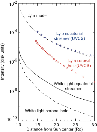
Figure 11.: Variation of the L$\alpha$ and white-light intensities (normalized to the disk-averaged intensities) with the distance to Sun center for two coronal regions: coronal hole and equatorial streamer. The L$\alpha$ data are from UVCS, the white-light data from S. Koutchmy (2006, private communication). Reproduced from Vial et al. (2007)fig8

The H$\alpha$ absorbed and emitted intensity is:

$$\ilabel{eq1}I^{H\alpha}(r_{0})=B_{23}~{}\frac{h\nu^{H\alpha}}{4\pi}\int_{-\infty}^{+\infty}n_{2}(s)\int_{0}^{+\infty}\int_{\Omega}I_{\mathrm{inc}}^{H\alpha}(\nu,\omega)\frac{\mathrm{d}\omega}{4\pi}\phi^{H\alpha}(\nu,s)\mathrm{d}\nu~{}\mathrm{d}s$$ (1)

The L$\alpha$ absorbed intensity is:

$$\ilabel{eq2}I^{L\alpha}(r_{0})=B_{12}~{}\frac{h\nu^{L\alpha}}{4\pi}\int_{-\infty}^{+\infty}n_{1}(s)\int_{0}^{+\infty}\int_{\Omega}I_{\mathrm{inc}}^{L\alpha}(\nu,\omega)\frac{\mathrm{d}\omega}{4\pi}\phi^{L\alpha}(\nu,s)\mathrm{d}\nu~{}\mathrm{d}s$$ (2)

The L$\alpha$ emitted intensity is:

$$\ilabel{eq3}I^{L\alpha}(r_{0})=A_{21}~{}\frac{h\nu^{L\alpha}}{4\pi}\int_{-\infty}^{+\infty}n_{2}(s)\mathrm{d}s\int_{0}^{+\infty}\phi(\lambda)\mathrm{d}\lambda$$ (3)

where $\phi(\nu,s)$ is the absorption profile at position $s$, where s is the distance of point $M$ along the ray taken from the impact point $P$ (at altitude $r_{0}$).
$I_{\mathrm{inc}}(\nu,\omega)$ (or $I_{\mathrm{inc}}(\lambda,\omega)$) is the incident radiation at position $M(s)$, depending on the frequency [$\nu$] (or wavelength [$\lambda$]) and solid angle [$\omega$].
With the transformation $\displaystyle\mathrm{d}s=\frac{r\mathrm{d}r}{\sqrt{r^{2}-r_{0}^{2}}}$, Equations (eq1), (eq2) and (eq3) become Volterra integral equations of the first kind. But the kernels are complex and include singularities. Consequently, we proceed with important simplifications where the quantity $\displaystyle\int I_{\mathrm{inc}}(\lambda,\omega)\frac{\mathrm{d}\omega}{4\pi}~{}\mathrm{d}\lambda~{}\phi(\lambda)$ $\displaystyle\Big{(}\mathrm{or}~{}\int I_{\mathrm{inc}}(\nu,\omega)~{}\frac{\mathrm{d}\omega}{4\pi}~{}\mathrm{d}\nu~{}\phi(\nu)\Big{)}$ is replaced in Equations (eq1) and (eq2) by
$<I_{\mathrm{emitted}}>\times w(r_{0})\times\mathrm{FWHM}$, where $w(r_{0})=0.5~{}\Big{(}1-\sqrt{1-\Big{(}\frac{R}{r_{0}}\Big{)}^{2}}\Big{)}$ is the dilution factor taken at $r_{0}$. Equation (eq1) becomes:

$$I^{H\alpha}(r_{0})=B_{23}~{}\frac{h\nu^{H\alpha}}{4\pi}\int_{-\infty}^{+\infty}n_{2}(s)~{}\mathrm{ds}~{}<I_{\mathrm{emitted}}^{H\alpha}>~{}w(r_{0})~{}\mathrm{FWHM}_{H\alpha}$$

where $<I_{\mathrm{emitted}}>$ is the chromospheric (incident) integrated emission that, when possible, we replace by the product of the half-intensity by the Full Width at Half Maximum (FWHM).
We have considered that $\displaystyle\phi^{H\alpha}(\nu,s)$ or $\displaystyle\phi^{H\alpha}(\lambda,s)$ depends (weakly) on temperature which is about $10^{6}$K. Then the Doppler width is $\displaystyle\Delta\lambda_{D}^{H\alpha}\approx 2.8$ Å and
$\mathrm{FWHM}(=2\sqrt{\log_{e}2}~{}\Delta\lambda_{D})=4.7$ Å. We also replace $\displaystyle\int n_{2}~{}\mathrm{d}s$ by $n_{2}(r_{0})~{}\Delta s$,
where $\Delta s$ is the LOS distance over which $n_{2}$ is significant.
The incident radiation is taken from David (1961) for H$\alpha$ and from Makarova and Kharitonov (1969) for the nearby continuum. We take an average value of 60 % of the continuum over a FWHM of 4.7 Å. Equation (eq1) becomes:

$$\ilabel{eq4}I^{H\alpha}(r_{0})=B_{23}~{}\frac{h\nu^{H\alpha}}{4\pi}~{}n_{2}(r_{0})~{}\Delta s~{}<I_{\mathrm{emitted}}^{H\alpha}>~{}w(r_{0})~{}\mathrm{FWHM}(H\alpha)$$ (4)

Similarly, (eq2) becomes:

$$I^{L\alpha}(r_{0})=B_{12}~{}\frac{h\nu^{L\alpha}}{4\pi}~{}n_{1}(r_{0})~{}\Delta s~{}<I_{\mathrm{emitted}}^{L\alpha}>~{}w(r_{0})~{}\mathrm{FWHM}(L\alpha)$$ (5)

Note that we take the same $\Delta s$ along which the densities ($n_{1}$, $n_{2}$, …) are significant. This is not different from computing the emission at position $P(r_{0})$.
Then, Equation (eq3) becomes:

$$\ilabel{eq6}I^{L\alpha}(r_{0})=A_{21}~{}\frac{h\nu^{L\alpha}}{4\pi}~{}n_{2}(r_{0})~{}\Delta s~{}\mathrm{FWHM}(L\alpha)$$ (6)

The ratio between Equations (eq4) and (eq6) gives:

$$\ilabel{eq7}\frac{I^{H\alpha}(r_{0})}{I^{L\alpha}(r_{0})}=\frac{B_{23}}{A_{21}}~{}\frac{\nu^{H\alpha}}{\nu^{L\alpha}}~{}<I_{\mathrm{emitted}}^{H\alpha}>~{}w(r_{0})~{}\frac{\mathrm{FWHM}(H\alpha)}{\mathrm{FWHM}(L\alpha)}$$ (7)

The L$\alpha$ emission is taken from Figure fig8 at 1.05 and 1.9 R_⊙.
With the respective values of $w(r)$ (0.35 at 1.05 R_⊙ and 0.075 at 1.9 R_⊙), the ratio $\displaystyle\frac{\mathrm{FWHM}(H\alpha)}{\mathrm{FWHM}(L\alpha)}$ taken at $10^{6}$ K as 9.3, we find, for a 4.7 Å bandpass, 107.5 and 0.23 erg s^-1cm^-2sr^-1 at 1.05 and 1.9 R_⊙ respectively. Table tab1 provides exact values which are about three times weaker at both altitudes. This agreement, which is well within an order of magnitude, is rather satisfactory when we take into account the many assumptions made in our analytical computation on one hand, and our use of coronal models that may well not represent reality, on the other hand. However, this computation has the advantage of providing a simple rule (Equation (eq7)) for deriving the H$\alpha$ intensity whenever and wherever the L$\alpha$ intensity is measured.

Acknowledgments

This paper is dedicated to Lola Salines who was murdered in Paris on 13 November 2015. The authors thank Pierre Gouttebroze, Iraïda Kim and Serge Koutchmy for useful comments. They deeply thank the referee for their comments which helped to improve the paper and clarify its aims.

Disclosure of Potential Conflict of Interest

The authors declare that they have no conflicts of interest.

References

- Allen (1977) Allen, K.W.: 1977, Astrophysical quantities., 3rd edn. London. ADS.
- Antonucci et al. (2012) Antonucci, E., Fineschi, S., Naletto, G., Romoli, M., Spadaro, D., Nicolini, G., Nicolosi, P., Abbo, L., Andretta, V., Bemporad, A., Auchère, F., Berlicki, A., Bruno, R., Capobianco, G., Ciaravella, A., Crescenzio, G., Da Deppo, V., D’Amicis, R., Focardi, M., Frassetto, F., Heinzel, P., Lamy, P.L., Landini, F., Massone, G., Malvezzi, M.A., Moses, J.D., Pancrazzi, M., Pelizzo, M.-G., Poletto, L., Schühle, U.H., Solanki, S.K., Telloni, D., Teriaca, L., Uslenghi, M.: 2012, Multi Element Telescope for Imaging and Spectroscopy (METIS) coronagraph for the Solar Orbiter mission. In: Space Telescopes and Instrumentation 2012: Ultraviolet to Gamma Ray, Proc. SPIE 8443, 844309. DOI. ADS.
- Anzer and Heinzel (1999) Anzer, U., Heinzel, P.: 1999, The energy balance in solar prominences. A&A 349, 974. ADS.
- Auchère (2005) Auchère, F.: 2005, Effect of the H I Ly Chromospheric Flux Anisotropy on the Total Intensity of the Resonantly Scattered Coronal Radiation. ApJ 622, 737. DOI. ADS.
- Bemporad, Matthaeus, and Poletto (2008) Bemporad, A., Matthaeus, W.H., Poletto, G.: 2008, Low-Frequency Ly Power Spectra Observed by UVCS in a Polar Coronal Hole. ApJ 677, L137. DOI. ADS.
- Bommier and Sahal-Brechot (1982) Bommier, V., Sahal-Brechot, S.: 1982, The Hanle effect of the coronal L-alpha line of hydrogen-Theoretical investigation. Sol. Phys. 78, 157. DOI. ADS.
- Bommier, Sahal-Brechot, and Leroy (1981) Bommier, V., Sahal-Brechot, S., Leroy, J.L.: 1981, Determination of the complete vector magnetic field in solar prominences, using the Hanle effect. A&A 100, 231. ADS.
- Ciaravella et al. (2003) Ciaravella, A., Raymond, J.C., van Ballegooijen, A., Strachan, L., Vourlidas, A., Li, J., Chen, J., Panasyuk, A.: 2003, Physical Parameters of the 2000 February 11 Coronal Mass Ejection: Ultraviolet Spectra versus White-Light Images. ApJ 597, 1118. DOI. ADS.
- Cranmer et al. (1999) Cranmer, S.R., Kohl, J.L., Noci, G., Antonucci, E., Tondello, G., Huber, M.C.E., Strachan, L., Panasyuk, A.V., Gardner, L.D., Romoli, M., Fineschi, S., Dobrzycka, D., Raymond, J.C., Nicolosi, P., Siegmund, O.H.W., Spadaro, D., Benna, C., Ciaravella, A., Giordano, S., Habbal, S.R., Karovska, M., Li, X., Martin, R., Michels, J.G., Modigliani, A., Naletto, G., O’Neal, R.H., Pernechele, C., Poletto, G., Smith, P.L., Suleiman, R.M.: 1999, An Empirical Model of a Polar Coronal Hole at Solar Minimum. ApJ 511, 481. DOI. ADS.
- David et al. (1998) David, C., Gabriel, A.H., Bely-Dubau, F., Fludra, A., Lemaire, P., Wilhelm, K.: 1998, Measurement of the electron temperature gradient in a solar coronal hole. A&A 336, L90. ADS.
- David (1961) David, K.-H.: 1961, Die Mitte-Rand Variation der Balmerlinien H-H auf der Sonnenscheibe. Mit 9 Textabbildungen. ZAp 53, 37. ADS.
- Derouich et al. (2010) Derouich, M., Auchère, F., Vial, J.C., Zhang, M.: 2010, Hanle signatures of the coronal magnetic field in the linear polarization of the hydrogen L line. A&A 511, A7. DOI. ADS.
- Dolei, Spadaro, and Ventura (2015) Dolei, S., Spadaro, D., Ventura, R.: 2015, Visible light and ultraviolet observations of coronal structures: physical properties of an equatorial streamer and modelling of the F corona. A&A 577, A34. DOI. ADS.
- Dolei et al. (2014) Dolei, S., Romano, P., Spadaro, D., Ventura, R.: 2014, Stereoscopic observations of the effects of a halo CME on the solar coronal structure. A&A 567, A9. DOI. ADS.
- Gabriel (1971) Gabriel, A.H.: 1971, Measurements on the Lyman Alpha Corona (Papers presented at the Proceedings of the International Symposium on the 1970 Solar Eclipse, held in Seattle, U. S. A. , 18-21 June, 1971.). Sol. Phys. 21, 392. DOI. ADS.
- Giordano et al. (2013) Giordano, S., Ciaravella, A., Raymond, J.C., Ko, Y.-K., Suleiman, R.: 2013, UVCS/SOHO catalog of coronal mass ejections from 1996 to 2005: Spectroscopic proprieties. J. Geophys. Res. (Space Physics) 118, 967. DOI. ADS.
- Goryaev et al. (2014) Goryaev, F., Slemzin, V., Vainshtein, L., Williams, D.R.: 2014, Study of Extreme-ultraviolet Emission and Properties of a Coronal Streamer from PROBA2/SWAP, Hinode/EIS and Mauna Loa Mk4 Observations. ApJ 781, 100. DOI. ADS.
- Gouttebroze, Heinzel, and Vial (1993) Gouttebroze, P., Heinzel, P., Vial, J.C.: 1993, The hydrogen spectrum of model prominences. A&AS 99, 513. ADS.
- Gunár (2014) Gunár, S.: 2014, Modelling of quiescent prominence fine structures. In: Schmieder, B., Malherbe, J.-M., Wu, S.T. (eds.) Nature of Prominences and their Role in Space Weather, IAU Symp. 300, 59. DOI. ADS.
- Hassler et al. (1994) Hassler, D.M., Strachan, L., Gardner, L.D., Kohl, J.L., Guhathakurta, M., Fisher, R.R., Strong, K.: 1994, Ly-alpha and white light observations of a CME during the Spartan 201-1 mission. In: Hunt, J.J. (ed.) Solar Dynamic Phenomena and Solar Wind Consequences, the Third SOHO Workshop, ESA-SP 373, 363. ADS.
- Heasley and Mihalas (1976) Heasley, J.N., Mihalas, D.: 1976, Structure and spectrum of quiescent prominences - Energy balance and hydrogen spectrum. ApJ 205, 273. DOI. ADS.
- Heinzel (2015) Heinzel, P.: 2015, Radiative Transfer in Solar Prominences. In: Vial, J.-C., Engvold, O. (eds.) Solar Prominences, Astrophys. Space Scien. Lib. 415, 103. DOI. ADS.
- Heinzel, Anzer, and Gunár (2005) Heinzel, P., Anzer, U., Gunár, S.: 2005, Prominence fine structures in a magnetic equilibrium. II. A grid of two-dimensional models. A&A 442, 331. DOI. ADS.
- Hyder and Lites (1970) Hyder, C.L., Lites, B.W.: 1970, H Doppler Brightening and Lyman- Doppler Dimming in Moving H Prominences. Sol. Phys. 14, 147. DOI. ADS.
- Kim et al. (2013a) Kim, I.S., Alexeeva, I.V., Bugaenko, O.I., Popov, V.V., Suyunova, E.Z.: 2013a, Near-Limb Zeeman and Hanle Diagnostics. Sol. Phys. 288, 651. DOI. ADS.
- Kim et al. (2013b) Kim, I.S., Popov, V.V., Lisin, D.V., Osokin, A.P.: 2013b, Observations of neutral hydrogen in the corona. Geomag. Aeron. 53, 901. DOI. ADS.
- Kohl et al. (1995) Kohl, J.L., Gardner, L.D., Strachan, L., Fisher, R., Guhathakurta, M.: 1995, SPARTAN 201 Coronal Spectroscopy During the Polar Passes of ULYSSES. Space Sci. Rev. 72, 29. DOI. ADS.
- Kohl et al. (2007) Kohl, J.L., Panasyuk, A., Cranmer, S.R., Gardner, L.D., Raymond, J.C.: 2007, Measurements of Coronal Proton Velocity Distributions. AGU Abs., A298. ADS.
- Koutchmy et al. (1994) Koutchmy, S., Belmahdi, M., Coulter, R.L., Demoulin, P., Gaizauskas, V., MacQueen, R.M., Monnet, G., Mouette, J., Noens, J.C., November, L.J.: 1994, CFHT eclipse observation of the very fine-scale solar corona. A&A 281, 249. ADS.
- Kramida et al. (2015) Kramida, A., Ralchenko, Y., Reader, J., (2015), N.T.: 2015, Atomic Spectra Database (version 5.3), physics.nist.gov/asd. National Institute of Standards and Technology, Gaithersburg, MD..
- Labrosse (2015) Labrosse, N.: 2015, Derivation of the Major Properties of Prominences Using NLTE Modelling. In: Vial, J.-C., Engvold, O. (eds.) Solar Prominences, Astrophys. Space Scien. Lib. 415, 131. DOI. ADS.
- Labrosse, Li, and Li (2006) Labrosse, N., Li, X., Li, B.: 2006, On the Lyman and lines in solar coronal streamers. A&A 455, 719. DOI. ADS.
- Labrosse et al. (2010) Labrosse, N., Heinzel, P., Vial, J.-C., Kucera, T., Parenti, S., Gunár, S., Schmieder, B., Kilper, G.: 2010, Physics of Solar Prominences: I-Spectral Diagnostics and Non-LTE Modelling. Space Sci. Rev. 151, 243. DOI. ADS.
- Leenaarts, Carlsson, and Rouppe van der Voort (2012) Leenaarts, J., Carlsson, M., Rouppe van der Voort, L.: 2012, The Formation of the H Line in the Solar Chromosphere. ApJ 749, 136. DOI. ADS.
- Lemaire et al. (2012) Lemaire, P., Vial, J.-C., Curdt, W., Schühle, U., Woods, T.N.: 2012, The solar hydrogen Lyman to Lyman line ratio. A&A 542, L25. DOI. ADS.
- Leroy (1981) Leroy, J.-L.: 1981, Simultaneous measurement of the polarization in H-alpha and D3 prominence emissions. Sol. Phys. 71, 285. DOI. ADS.
- Li, Li, and Labrosse (2006) Li, B., Li, X., Labrosse, N.: 2006, A global 2.5-dimensional three fluid solar wind model with alpha particles. J. Geophys. Res. (Space Physics) 111, A08106. DOI. ADS.
- Lin, Penn, and Tomczyk (2000) Lin, H., Penn, M.J., Tomczyk, S.: 2000, A New Precise Measurement of the Coronal Magnetic Field Strength. ApJ 541, L83. DOI. ADS.
- Maccari et al. (1999) Maccari, L., Noci, G., Modigliani, A., Romoli, M., Fineschi, S., Kohl, J.L.: 1999, Ly- Observation of a Coronal Streamer with UVCS/SOHO. Space Sci. Rev. 87, 265. DOI. ADS.
- Makarova and Kharitonov (1969) Makarova, E.A., Kharitonov, A.V.: 1969, Mean Absolute Energy Distribution in the Solar Spectrum from 1800 Å to 4 mm, and the Solar Constant. Soviet Astron. 12, 599. ADS.
- Marsch et al. (1999) Marsch, E., Tu, C.-Y., Heinzel, P., Wilhelm, K., Curdt, W.: 1999, Proton and hydrogen temperatures at the base of the solar polar corona. A&A 347, 676. ADS.
- Mierla et al. (2011) Mierla, M., Chifu, I., Inhester, B., Rodriguez, L., Zhukov, A.: 2011, Low polarised emission from the core of coronal mass ejections. A&A 530, L1. DOI. ADS.
- Miralles et al. (1999) Miralles, M.P., Strachan, L., Gardner, L.D., Dobryzcka, D., Ko, Y.-K., Michels, J., Panasyuk, A., Suleiman, R., Kohl, J.L.: 1999, Streamer HI Ly- Line Profiles During the Spartan 201-05/SOHO Coordinated Observations. In: Wilson, A., et al.(eds.) Magnetic Fields and Solar Processes, ESA-SP 448, 1193. ADS.
- Noci, Kohl, and Withbroe (1987) Noci, G., Kohl, J.L., Withbroe, G.L.: 1987, Solar wind diagnostics from Doppler-enhanced scattering. ApJ 315, 706. DOI. ADS.
- Peter et al. (2012) Peter, H., Abbo, L., Andretta, V., Auchère, F., Bemporad, A., Berrilli, F., Bommier, V., Braukhane, A., Casini, R., Curdt, W., Davila, J., Dittus, H., Fineschi, S., Fludra, A., Gandorfer, A., Griffin, D., Inhester, B., Lagg, A., Degl’Innocenti, V. E. L. andMaiwald, Sainz, R.M., Pillet, V.M., Matthews, S., Moses, D., Parenti, S., Pietarila, A., Quantius, D., Raouafi, N.-E., Raymond, J., Rochus, P., Romberg, O., Schlotterer, M., Schühle, U., Solanki, S., Spadaro, D., Teriaca, L., Tomczyk, S., Bueno, J.T., Vial, J.-C.: 2012, Solar magnetism eXplorer (SolmeX). Exploring the magnetic field in the upper atmosphere of our closest star. Exp. Astron. 33, 271. DOI. ADS.
- Poland and Munro (1976) Poland, A.I., Munro, R.H.: 1976, Interpretation of broad-band polarimetry of solar coronal transients - Importance of H-alpha emission. ApJ 209, 927. DOI. ADS.
- Raymond et al. (1997) Raymond, J.C., Kohl, J.L., Noci, G., Antonucci, E., Tondello, G., Huber, M.C.E., Gardner, L.D., Nicolosi, P., Fineschi, S., Romoli, M., Spadaro, D., Siegmund, O.H.W., Benna, C., Ciaravella, A., Cranmer, S., Giordano, S., Karovska, M., Martin, R., Michels, J., Modigliani, A., Naletto, G., Panasyuk, A., Pernechele, C., Poletto, G., Smith, P.L., Suleiman, R.M., Strachan, L.: 1997, Composition of Coronal Streamers from the SOHO Ultraviolet Coronagraph Spectrometer. Sol. Phys. 175, 645. DOI. ADS.
- Schrijver et al. (2015) Schrijver, C.J., Kauristie, K., Aylward, A.D., Denardini, C.M., Gibson, S.E., Glover, A., Gopalswamy, N., Grande, M., Hapgood, M., Heynderickx, D., Jakowski, N., Kalegaev, V.V., Lapenta, G., Linker, J.A., Liu, S., Mandrini, C.H., Mann, I.R., Nagatsuma, T., Nandy, D., Obara, T., Paul O’Brien, T., Onsager, T., Opgenoorth, H.J., Terkildsen, M., Valladares, C.E., Vilmer, N.: 2015, Understanding space weather to shield society: A global road map for 2015-2025 commissioned by COSPAR and ILWS. Adv. Space Res. 55, 2745. DOI. ADS.
- Spadaro et al. (2007) Spadaro, D., Susino, R., Ventura, R., Vourlidas, A., Landi, E.: 2007, Physical parameters of a mid-latitude streamer during the declining phase of the solar cycle. A&A 475, 707. DOI. ADS.
- Susino et al. (2008) Susino, R., Ventura, R., Spadaro, D., Vourlidas, A., Landi, E.: 2008, Physical parameters along the boundaries of a mid-latitude streamer and in its adjacent regions. A&A 488, 303. DOI. ADS.
- Tomczyk et al. (2008) Tomczyk, S., Card, G.L., Darnell, T., Elmore, D.F., Lull, R., Nelson, P.G., Streander, K.V., Burkepile, J., Casini, R., Judge, P.G.: 2008, An Instrument to Measure Coronal Emission Line Polarization. Sol. Phys. 247, 411. DOI. ADS.
- Vial (1970) Vial, J.C.: 1970, Intensity Distribution in the LYMAN- Line at the Solar Limb. In: Muller, R., Houziaux, L., Butler, H.E. (eds.) Ultraviolet Stellar Spectra and Related Ground-Based Observations, IAU Symp. 36, 260. ADS.
- Vial et al. (1992) Vial, J.-C., Koutchmy, S., Monnet, G., Sovka, J., Clark, C., Salmon, D., Purves, N., Sydserff, P., Coulder, R., November, L.: 1992, Evidence of plasmoid ejection in the corona from 1991 eclipse observations with the Canada-France-Hawaii telescope. In: Dame, L., Guyenne, T.-D. (eds.) ESA Special Publication, ESA-SP 344, 87. ADS.
- Vial et al. (2007) Vial, J.-C., Auchère, F., Chang, J., Fang, C., Gan, W.Q., Klein, K.-L., Prado, J.-Y., Trottet, G., Wang, C., Yan, Y.H.: 2007, SMESE: A SMall Explorer for Solar Eruptions. Adv. Space Res. 40, 1787. DOI. ADS.
- Withbroe et al. (1982) Withbroe, G.L., Kohl, J.L., Weiser, H., Munro, R.H.: 1982, Probing the solar wind acceleration region using spectroscopic techniques. Space Sci. Rev. 33, 17. DOI. ADS.
- Zangrilli et al. (1999) Zangrilli, L., Nicolosi, P., Poletto, G., Noci, G., Romoli, M., Kohl, J.L.: 1999, Latitudinal properties of the Lyman alpha and O VI profiles in the extended solar corona. A&A 342, 592. ADS.
- Zhukov et al. (2000) Zhukov, A.N., Veselovsky, I.S., Koutchmy, S., Delannée, C.: 2000, Coronal plasmoid dynamics. II. The nonstationary fine structure. A&A 353, 786. ADS.