Asymptotic Analysis of Equivalences and Core-Structures in Kronecker-Style Graph Models

Abstract

Growing interest in modeling large, complex networks has spurred significant research into generative graph models. These models not only allow users to gain insight into the processes underlying networks, but also provide synthetic data which allows algorithm scalability testing and addresses privacy concerns. Kronecker-style models (e.g. SKG and R-MAT) are often used due to their scalability and ability to mimic key properties of real-world networks (e.g. diameter and degree distribution). Although a few papers theoretically establish these models’ behavior for specific parameters, many claims used to justify the use of these models in various applications are supported only by empirical evaluations. In this work, we prove several results using asymptotic analysis which illustrate that empirical studies may not fully capture the true behavior of the models.

Paramount to the widespread adoption of Kronecker-style models was the introduction of a linear-time edge-sampling variant (R-MAT), which existing literature typically treats as interchangeable with SKG. We prove that although several R-MAT formulations are asymptotically equivalent, their behavior diverges from that of SKG. Further, we show these results are experimentally observable even at relatively small graph sizes. Second, we consider a case where asymptotic analysis reveals unexpected behavior within a given model. One of the criticisms of using Kronecker-style models has been that they are unable to generate the deep core-structures commonly observed in real-world data. We prove that in fact, for some parameter values, all the Kronecker-style models generate graphs whose maximum core depth grows as a function of the size of the network—including in the region of the parameter space most commonly used in prior work. Our results also illustrate why this behavior may be difficult to observe for moderate graph sizes, and highlight the dangers of extrapolating model-wide claims from empirical results.

I Introduction

The rapidly increasing availability of large relational data sets has brought network science to the forefront of a diverse set of fields like business, social sciences, natural sciences, and engineering. Due to privacy restrictions and the desire to have testing data at larger scales, generating synthetic data from random graph models to evaluate new algorithms or techniques has become a common practice. A significant amount of research has focused on creating generative models that produce networks whose properties mimic those of real data sets. One popular family of such models, which we refer to as Kronecker-style models, is based on using a small “seed” or initiator matrix to generate a fractal structure of edge probabilities. This family includes stochastic Kronecker graphs ($\mathrm{SKG}$) [1, 2], the Recursive-MATrix ($\mathrm{R\text{-}M\kern-1.00006ptAT}$) generator  [3], and several variants of each [4, 5].

The widespread adoption [6, 7, 8, 9, 10] of Kronecker-style models has been motivated by empirical evidence showing the generated networks replicate several important properties of real world networks, including degree and eigenvalue distributions, diameter, and density [1, 2]. Further, the initiator matrix parameters can be learned from a real-world network using the algorithm KronFit [11]; empirical evaluation shows that using the fitted parameters on a dozen datasets, synthetic $\mathrm{SKG}$ graphs mimic real-world degree distributions and small diameters. To complement the work measuring properties of generated data, a number of papers have proven explicit expressions for computing the expected value of some graph invariant (e.g. degree distribution [12] and number of isolated vertices [5]). Finally, a few papers have considered the limiting behavior of these models—characterizing the emergence of a giant component and proving constant diameter [13], and proving that $\mathrm{SKG}$ generally cannot generate graphs with a power-law degree distribution [14].

Here we show that asymptotic analysis of Kronecker-style models not only offers formal guarantees on limiting behavior, but practically-relevant restrictions on their usage. Specifically, we focus on two properties of these models: (1) equivalence/inequivalence among variants and (2) their core-periphery structure, as measured by degeneracy.

Our first result addresses the common practice of using distinct variations of Kronecker-style models interchangeably, despite the lack of formal proofs of equivalence in the literature. A recent paper of Moreno et al. [15] challenged these assumptions and proved that without careful consideration, two Kronecker-style models will not necessarily sample from the same statistical distribution given analogous input parameters. We show in Section III that in the limit, several widely-used variants of the $\mathrm{R\text{-}M\kern-1.00006ptAT}$ models are indeed equivalent (Theorem 1). However, we also prove that their edge probabilities diverge from those of $\mathrm{SKG}$, and show these differences are experimentally observable even at relatively small graph sizes.

Our second contribution provides insight into the core-periphery structure of graphs generated by these models, as measured by the degeneracy. Low degeneracy means the graph has no region (subgraph) that is “too dense”, and is an observed property of many real-world networks. Empirical studies [5] have suggested that the degeneracy of Kronecker-style models cannot grow large without increasing the number of isolated vertices. Our proofs in Section IV disprove this, showing that for a fixed average degree, these models produce graphs whose degeneracy grows asymptotically with the number of vertices irrespective of the number of isolated vertices. However, our results also imply that this asymptotic behavior is slow to appear, preventing the occurrence of deep cores even for graphs with hundreds of thousands of vertices (and causing misleading empirical evidence).

II Preliminaries

We assume that all graphs are simple (no parallel edges or self-loops) and undirected unless otherwise specified. Directed graphs will be denoted by an arrow (e.g. $\vec{G}$). Let $\mathcal{G}_{n}$ denote the set of all $n$-vertex graphs. A random graph model is a sequence of probability measures $(\operatorname{\mathbb{P}}_{n})_{n\in\mathbb{N}}$ over the space $(\mathcal{G}_{n},2^{\mathcal{G}_{n}})$. For simplicity, we use $\operatorname{\mathbb{P}}$ as the probability measure with the understanding that it refers to a concrete random graph model that will be apparent from the context.

For convenience we consider $n$-vertex graphs whose vertices are numbered $0$ to $n-1$ and represented by binary bitstrings. This convention will allow us to derive the (relative) probability of an edge in a Kronecker-style model from the positions of ones in its endpoints. For bitstrings $i,j$ of equal length we use $\#ab(ij)$ to denote the number of positions in which $a$ occurs in $i$ when $b$ occurs in $j$, i.e.,

$$\#ab(ij)=|\{x~{}:~{}i[x]=a~{}\wedge~{}j[x]=b\}|\text{ for }a,b\in\{0,1\}.$$

II-A Kronecker-style Models

We now define the Kronecker-style models, including a new formulation $\mathrm{R\text{-}M\kern-1.00006ptAT}^{\$}$ used in our analysis. For reference, Table I summarizes the notation defined below.

Symbol	Model Name
$\mathrm{SKG}$	Stochastic Kronecker
$\mathrm{R\text{-}M\kern-0.90005ptAT}^{\ominus}$	$\mathrm{R\text{-}M\kern-0.90005ptAT}$ with arc erasures
$\mathrm{R\text{-}M\kern-0.90005ptAT}^{\oplus}$	$\mathrm{R\text{-}M\kern-0.90005ptAT}$ with arc rethrows
$\mathrm{R\text{-}M\kern-0.90005ptAT}^{\$}$	$\mathrm{R\text{-}M\kern-0.90005ptAT}$ simulated by coin-flips

TABLE I: Summary of Kronecker-style models.

Stochastic Kronecker: In 2005, Leskovec et al. [1] introduced the Stochastic Kronecker random graph generator ($\mathrm{SKG}$) as a means of modeling real-world data. Taking an initiator matrix $M_{1}$ with values in the interval $[0,1]$ (not necessarily summing to $1$) and a natural number $k$, $\mathrm{SKG}$ starts by deterministically generating a probability matrix $M_{k}$, such that $M_{k}=M_{k-1}\otimes M_{1}$, where $\otimes$ is the tensor (Kronecker) product. A directed graph can then be sampled from $M_{k}$ by flipping one biased coin per matrix entry to obtain an adjacency matrix. In keeping with prior work, we assume $M_{1}=\bigl{(}\begin{smallmatrix}a&b\\ c&d\end{smallmatrix}\bigr{)}$; such a $2\times 2$ initiator matrix has been most widely adopted in the literature (including [5, 12, 13, 14]) after experiments found it generates synthetic graphs that most closely match real-world data [11].

R-MAT erasure and rethrow models: Independent of $\mathrm{SKG}$, in 2004, Chakrabarti et al. [3] introduced the Recursive MATrix ($\mathrm{R\text{-}M\kern-1.00006ptAT}$) graph generator. Similar to $\mathrm{SKG}$, $\mathrm{R\text{-}M\kern-1.00006ptAT}$ starts with an initiator matrix $M$ and natural number $k$, with the restriction that $M=\bigl{(}\begin{smallmatrix}\alpha&\beta\\ \gamma&\delta\end{smallmatrix}\bigr{)}$ and $\alpha+\beta+\gamma+\delta=1$; we will also assume (without loss of generality) that $\alpha\geqslant\beta,\gamma,\delta$. A $2^{k}\times 2^{k}$ directed adjacency matrix is then constructed by iteratively “throwing” $m$ arcs recursively into quadrants of the adjacency matrix based on the probabilities from $M$; we call this method the general R-MAT process.

Formally, starting with a graph $\vec{G}^{0}$ on $2^{k}$ vertices with no arcs, at each step $1\leqslant i\leqslant m$ we generate a random arc $e_{i}$ by flipping two biased coins $C_{1},C_{2}$ for $k$ rounds where $\operatorname{\mathbb{P}}[C_{1}=1]=\gamma+\delta$ and $\operatorname{\mathbb{P}}[C_{2}=1]=\beta+\delta$. The head of $e_{i}$ is the bitstring formed by concatenating the results of $C_{2}$, and the tail is obtained using $C_{1}$. We then either add $e_{i}$ to the graph or rethrow the edge (detailed below) to obtain $\vec{G}^{i}$.

The probability of an arc being selected in a single step is a function of the bitstrings of its endpoints. For vertices $u,v$ we define the weight of the (potential) arc $uv$ as

$$\omega_{uv}=\alpha^{\#00(uv)}\beta^{\#01(uv)}\gamma^{\#10(uv)}\delta^{\#11(uv)}.$$ (1)

Note that the probability of an arc existing in $\vec{G}^{m}$ is not necessarily its weight; rather, the probability can be computed from its weight and proper model-dependent scaling.

Given that we are generating simple graphs and a thrown arc may land in an occupied cell, we now define two existing implementations of the general $\mathrm{R\text{-}M\kern-1.00006ptAT}$ process. In the erasure model (denoted by $\mathrm{R\text{-}M\kern-1.00006ptAT}^{\ominus}$), the repeated arc is ignored, resulting in a generated graph with strictly less arcs than the number thrown. In the rethrow model (denoted by $\mathrm{R\text{-}M\kern-1.00006ptAT}^{\oplus}$), this arc is “rethrown” (flipping another $k$ pairs of coins) until it lands in an unoccupied cell. These two models are not strictly identical, since the probability distribution across unoccupied cells changes with each added arc in the rethrow model. $\mathrm{R\text{-}M\kern-1.00006ptAT}^{\ominus}$ is equivalent to the original formulation of the $\mathrm{R\text{-}M\kern-1.00006ptAT}$ model [3], and $\mathrm{R\text{-}M\kern-1.00006ptAT}^{\oplus}$ is consistent with the description of the $\mathrm{R\text{-}M\kern-1.00006ptAT}$ model in [2].

Converting parameters between SKG and R-MAT:
Historically, $\mathrm{R\text{-}M\kern-1.00006ptAT}$ has been treated as an $O(m)$ run time drop-in replacement for $\mathrm{SKG}$ (e.g., in [2, 5, 16]), but the details of converting parameters between models require some care. Let $\bigl{(}\begin{smallmatrix}a&b\\ c&d\end{smallmatrix}\bigr{)}$ be a $\mathrm{SKG}$ initiator matrix, then each arc $uv$ is added independently at random with probability

$$a^{\#00(uv)}b^{\#01(uv)}c^{\#10(uv)}d^{\#11(uv)}$$

and the expected number of arcs in the final graph is

$$m=(a+b+c+d)^{k}.$$

This formulation suggests the following translation between the $\mathrm{R\text{-}M\kern-1.00006ptAT}$ and $\mathrm{SKG}$ parameters. Suppose we want a graph with $n=2^{k}$ vertices and $m$ arcs. Let $\mu=m/2^{k}$ (i.e. the edge density), then we introduce a scaling parameter $\theta$ where $\bigl{(}\begin{smallmatrix}a&b\\ c&d\end{smallmatrix}\bigr{)}=\theta\bigl{(}\begin{smallmatrix}\alpha&\beta\\ \gamma&\delta\end{smallmatrix}\bigr{)}$. To compute $\theta$ we match up the expected number of edges of the models:

$$\mu\cdot 2^{k}=(a+b+c+d)^{k}=\theta^{k}(\alpha+\beta+\gamma+\delta)^{k}=\theta^{k}.$$

Therefore our scaling parameter is $\theta=2\mu^{1/k}$. Table II contains several $\mathrm{R\text{-}M\kern-1.00006ptAT}$ initiator matrices that were derived from $\mathrm{SKG}$ initiators fitted to real-world networks [2] using this conversion.

Note that in order to satisfy $\mathrm{SKG}$’s constraint that $a\leqslant 1$ (and given that $\alpha>\beta,\gamma,\delta$) we require that

$$\theta\alpha=\mu^{1/k}2\alpha\leqslant 1\implies\alpha\leqslant\frac{1}{2}\mu^{-1/k}.$$

This latter term converges to $1/2$ when $k\to\infty$ and $\mu$ is a constant independent of $n$. Since it is generally accepted that real-world networks are sparse, we will restrict ourselves to constant $\mu$ in the rest of this paper. In conclusion, the translation from $\mathrm{R\text{-}M\kern-1.00006ptAT}$ to $\mathrm{SKG}$ parameters is possible whenever $\alpha<1/2$, $\mu$ is a constant, and $k$ is large enough. This restriction on $\alpha$ has another interpretation: for $\alpha\geqslant 1/2$, $\mathrm{SKG}$ generates in expectation a sublinear number of arcs. Accordingly, in this regime $\mathrm{SKG}$ cannot possibly match up with the $\mathrm{R\text{-}M\kern-1.00006ptAT}$ model.

A new R-MAT model: In addition to the parameter space limitations, the arc generation process differs significantly between $\mathrm{SKG}$ and $\mathrm{R\text{-}M\kern-1.00006ptAT}$. Specifically, arcs occur in $\mathrm{SKG}$ independently while the existing $i-1$ arcs influence the placement of the $i^{\text{th}}$ arc in $\mathrm{R\text{-}M\kern-1.00006ptAT}^{\oplus}$ and $\mathrm{R\text{-}M\kern-1.00006ptAT}^{\ominus}$. To study whether this difference in mechanics results in dissimilar models, we introduce a new coin-flipping model, $\mathrm{R\text{-}M\kern-1.00006ptAT}^{\$}$. This model is not intended for practical usage since sampling from it requires $O(n^{2})$ iterations, but it is useful for mathematical analysis and to bridge the gap between the previous $\mathrm{R\text{-}M\kern-1.00006ptAT}$ models and $\mathrm{SKG}$.

First, note that the probability of an arc $uv$ occurring $t$ times in the $\mathrm{R\text{-}M\kern-1.00006ptAT}$ process follows the binomial law

$$\operatorname{\mathbb{P}}[|\{e_{i}\colon e_{i}=uv\}|=t] ={m\choose t}(\omega_{uv})^{t}(1-\omega_{uv})^{m-t}$$

where $\omega_{uv}$ is defined in Equation 1. Therefore the arc $uv$ exists after $m$ arcs have been thrown with probability

$$\operatorname{\mathbb{P}}[e\in\vec{G}^{m}]=1-(1-\omega_{uv})^{m}.$$

Utilizing this fact, we define the $\mathrm{R\text{-}M\kern-1.00006ptAT}^{\$}$ model:

Definition 1 ($\mathrm{R\text{-}M\kern-1.00006ptAT}^{\$}$).

Given an initiator matrix $M=\bigl{(}\begin{smallmatrix}\alpha&\beta\\ \gamma&\delta\end{smallmatrix}\bigr{)}$ with $\alpha,\beta,\gamma,\delta\geqslant 0$ and $\alpha+\beta+\gamma+\delta=1$, a natural number $k$, and a positive real number $\mu$, $\mathrm{R\text{-}M\kern-1.00006ptAT}^{\$}$ generates a graph with $2^{k}$ vertices by flipping every potential arc $uv$ independently at random with probability $1-(1-\omega_{uv})^{m}$.

Network	$n$	$\mu$	$\mathrm{R\text{-}M\kern-1.00006ptAT}$ initiator
AS-NEWMAN	$22963$	$4.22$	$[.432,.269;.269,.009]$
AS-ROUTEVIEWS	$6474$	$4.09$	$[.442,.255;.255,.022]$
BIO-PROTEINS	$4626$	$6.40$	$[.364,.275;.275,.031]$
CA-DBLP	$425957$	$6.33$	$[.453,.139;.139,.260]$
CA-GR-QC	$5242$	$5.53$	$[.435,.107;.107,.301]$
CA-HEP-PH	$12008$	$19.74$	$[.401,.175;.175,.194]$
CA-HEP-TH	$9877$	$5.26$	$[.441,.120;.120,.259]$
EMAIL-INSIDE	$986$	$32.58$	$[.352,.272;.272,.091]$
ANSWERS	$598314$	$3.07$	$[.469,.181;.195,.117]$
ATP-GR-QC	$19177$	$1.36$	$[.441,.124;.108,.285]$
BLOG-NAT05-6M	$31600$	$8.59$	$[.433,.246;.217,.096]$
BLOG-NAT06ALL	$32443$	$9.83$	$[.429,.248;.222,.095]$
CIT-HEP-PH	$30567$	$11.41$	$[.422,.186;.151,.223]$
CIT-HEP-TH	$27770$	$12.70$	$[.417,.185;.146,.226]$
DELICIOUS	$205282$	$2.13$	$[.479,.157;.167,.187]$
EPINIONS	$75879$	$6.71$	$[.444,.237;.213,.057]$
FLICKR	$584207$	$6.09$	$[.455,.216;.221,.066]$
GNUTELLA-25	$22687$	$2.41$	$[.351,.233;.308,.086]$
GNUTELLA-30	$36682$	$2.41$	$[.355,.231;.298,.084]$
WEB-NOTREDAME	$325729$	$4.60$	$[.460,.190;.208,.105]$

TABLE II: Initiator matrices of the 20 networks fitted to the $\mathrm{SKG}$ model in [2], converted to $\mathrm{R\text{-}M\kern-1.00006ptAT}$ initiator matrices. The upper half of the networks are undirected and hence have a symmetric initiator. We see that the densities are consistently small which supports the common assumption that $\mu$ is a constant independent of the graph size.

II-B Analytical tools

We use the following tools for asymptotic analysis:

Hamming slices: Since the bitstring representation of the vertices in Kronecker-style models encodes information about the edges between them, it will be useful to group the vertices by properties of their bitstrings. The Hamming weight of a vertex is the number of ones in its bitstring label. We define a Hamming slice $\mathcal{F}_{\ell}$ to be the set of all vertices whose bitstrings have Hamming weight exactly $\ell$. We also denote $\mathcal{F}_{\leqslant\ell}$ and $\mathcal{F}_{\geqslant\ell}$ as the set of vertices with bitstrings at most and at least Hamming weight $\ell$, respectively.

Asymptotic equivalence: Two random graph models $(\operatorname{\mathbb{P}}_{n}),(\mathbb{Q}_{n})$ are asymptotically equivalent if for every sequence of events $(\mathcal{E}_{n}\mid\mathcal{E}_{n}\in 2^{\mathcal{G}_{n}})_{n\in\mathbb{N}}$ it holds that

$$\lim_{n\to\infty}\operatorname{\mathbb{P}}_{n}[\mathcal{E}_{n}]-\mathbb{Q}_{n}[\mathcal{E}_{n}]=0.$$

Concentration inequalities: To show that the invariants of our graphs do not deviate far from their expected values, we use Chernoff–Hoeffding bounds.

Chernoff–Hoeffding ([17]).

Let $\{X_{i}\}_{i\in[n]}$ be random binary variables with associated success probabilities $\{p_{i}\}_{i\in[n]}$. Let further $\xi=\operatorname{\mathbb{E}}[\sum_{i}X_{i}]$. Then for every $\delta>0$ it holds that

$$\Pr\left[\sum_{i}X_{i}\geqslant(1+\delta)\xi\right]\leqslant\left(\frac{e^{\delta}}{(1+\delta)^{1+\delta}}\right)^{\xi}.$$

A common situation will be that $\xi$ tends towards zero as $n$ increases. Choosing some constant $c$ for which we want to obtain a bound, we let $c=(1+\delta)\xi$ from which we derive that $\delta\xi=c-\xi$ and $1+\delta=c/\xi$. We thus use the following reformulation of this bound:

$$\Pr\left[\sum_{i}X_{i}\geqslant c\right]\leqslant\frac{e^{\delta\xi}}{(1+\delta)^{(1+\delta)\xi}}=\frac{(e\xi)^{c}}{e^{\xi}c^{c}}\leqslant\left(\frac{e\xi}{c}\right)^{c}.$$

Binomial Coefficients: We also use the following bound on binomial coefficients based on Stirling’s approximation:

$$\frac{\sqrt{\pi}}{2}\Gamma(\tau)\leqslant{n\choose\tau n}\leqslant\Gamma(\tau)~{}\text{where}~{}\Gamma(\tau)=\frac{2^{nH(\tau)}}{\sqrt{2\pi n\tau(1{-}\tau)}},$$

and $H(x)=-\log_{2}(x^{x}(1-x)^{1-x})$ is the binary entropy function.

Degeneracy, cores, and dense subgraphs: Recent work on community structure in complex networks has pointed to some sort of “core-periphery” structure in many real networks (e.g. [18, 19, 20]), often exemplified using the $k$-core decomposition, a popular tool in visualization and social network analysis (see e.g. [21, 22, 23, 24, 25]).

The $k$-core of a graph is the maximal induced subgraph in which all vertices have degree at least $k$. The core-periphery structure of a network is often characterized in terms of the depth of its core-decomposition (largest $k$ such that the $k$-core is non-empty), an invariant known as the degeneracy. Both the degeneracy of a graph and its core decomposition can be computed in $O(m)$ time using an algorithm by Batagelj and Zaversnik [26]. In Section IV, we analyze the degeneracy of Kronecker-style models, using the following equivalent definition where needed:

Definition 2 (Degeneracy).

A graph $G$ is said to be $d$-degenerate if every (induced) subgraph has a vertex of degree at most $d$. The smallest $d$ for which $G$ is $d$-degenerate is the degeneracy of $G$.

In particular, all subgraphs of a $d$-degenerate graph are sparse; in the contrapositive this means that the existence of a subgraph of density $>d$ implies that the host graph is not $d$-degenerate. In the asymptotic setting, a dense subgraph is a sequence of subgraphs whose edge density diverges in the limit; the existence of such a substructure implies that for every integer $d$ the generated graphs past a certain threshold size are not $d$-degenerate. We will call graph models that contain dense subgraphs asymptotically dense.

II-C Repeatability

All experiments in this paper can be replicated with the code available at http://dl.dropboxusercontent.com/s/vfzvk72gpqbmhc9/asymptotic_kronecker.zip. This includes random graph model implementations, the random seeds used to generate the data used in this manuscript, and code to calculate and plot the relevant graph invariants. All code is written in Python; we recommend running with pypy to reduce runtimes.

III Relationships of Kronecker-style Models

We begin this section by proving that all of the aforementioned variants of $\mathrm{R\text{-}M\kern-1.00006ptAT}$ are equivalent asympotically. We then show that equivalent input parameters to $\mathrm{R\text{-}M\kern-1.00006ptAT}^{\$}$ and $\mathrm{SKG}$ do not generate equal probability distributions over the arcs. To further validate this proof, we provide an empirical result highlighting the difference between the models.

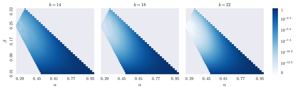
Figure 1: Proportion of arcs requiring a rethrow in $\mathrm{R\text{-}M\kern-1.00006ptAT}^{\oplus}$ as a function of $k$, $\alpha$, and $\beta$, averaged over ten graphs for each parameter value. All graphs were generated with $\mu=4$ and $\gamma=\beta$, fixing $\delta=1-\alpha-2\beta$.

III-A Equivalence of $\mathrm{R\text{-}M\kern-1.00006ptAT}$ variants

In this section, we show the following equivalence between the three $\mathrm{R\text{-}M\kern-1.00006ptAT}$ variants:

Theorem 1.

For parameters $\bigl{(}\begin{smallmatrix}\alpha&\beta\\ \gamma&\delta\end{smallmatrix}\bigr{)}$ where at least three entries are non-zero and $\mu\leqslant\log(n)/2$ the models $\mathrm{R\text{-}M\kern-1.00006ptAT}^{\ominus}$, $\mathrm{R\text{-}M\kern-1.00006ptAT}^{\oplus}$ and $\mathrm{R\text{-}M\kern-1.00006ptAT}^{\$}$ are asymptotically equivalent for appropriate scalings of the parameter $\mu$.

To prove this, we first establish that—in the sparse case—the erasure and rethrow models result asymptotically in the same process (Lemma 3, which uses Lemmas 1 and 2 to bound the number of rethrows). Equivalence with the coin-flipping model then follows easily in Lemma 4 using the edge probabilities defined in the general $\mathrm{R\text{-}M\kern-1.00006ptAT}$ process.

We start by estimating the probability that an arc lands on an occupied cell and therefore is handled differently in the erasure and rethrow models. In the remainder of this section, we fix an initiator matrix $\bigl{(}\begin{smallmatrix}\alpha&\beta\\ \gamma&\delta\end{smallmatrix}\bigr{)}$ and let  $\rho_{1}\geqslant\rho_{2}\geqslant\rho_{3}\geqslant\rho_{4}$ be its entries ordered by size. As before we denote by $k$ the number of Kronecker-multiplications and by $\mu$ the density parameter. The following lemma holds even when for a superlinear number of arcs and we state it in that generality, however, our subsequent application will again assume a linear number of arcs.

Lemma 1.

Let $\vec{G}$ be a graph on $n=2^{k}$ vertices with $cn$ arcs for $1\leqslant c\leqslant k/2$. There exists a function $f$ depending on $\rho_{1},\rho_{2}$ and $\rho_{3}$ such that

$$\sum_{e\in\vec{G}}\omega_{e}\leqslant(\rho_{1}+\rho_{2})^{k}\left(\rho_{3}+f(c)\right).$$

Proof.

The number of weights that only consist of the largest factors $\rho_{1}$ and $\rho_{2}$ is exactly $2^{k}=n$. For $c=1$, we have that at most a total weight of

$$\sum_{i=0}^{k}{k\choose i}\rho_{1}^{i}\rho_{2}^{k-i}=(\rho_{1}+\rho_{2})^{k}$$

is occupied by arcs in $\vec{G}$. We take these highest weights and replace up to $g$ positions with $\rho_{3}$ in order to increase maximum weight covered by $cn$ arcs: this provides us with at least

$$\phantom{{}={}}\sum_{j=0}^{g}{k\choose j}\sum_{i=0}^{k-j}{k-j\choose i}=\sum_{j=0}^{g}{k\choose j}2^{k-j}$$

$$\geqslant 2^{k}+2^{k}\sum_{j=1}^{g}\left(\frac{k}{2j}\right)^{j}\geqslant 2^{k}\left(1+\frac{gk}{2}\right).$$

arcs whose weights only consist of factors $\rho_{1},\rho_{2}$ and up to $g$ factors $\rho_{3}$. In order to now bound the total weight such arcs can occupy, we solve for $g$:

$$1+\frac{gk}{2}=c\iff g=2\frac{c-1}{k}.$$

The total weight of the $cn$ arcs in $\vec{G}$ is therefore at most

$$\phantom{{}\leqslant{}}\sum_{j=0}^{g}{k\choose j}\rho_{3}^{j}\sum_{i=0}^{k-j}{k-j\choose i}\rho_{1}^{i}\rho_{2}^{k-j-i}$$

$$=\sum_{j=0}^{g}{k\choose j}\rho_{3}^{j}(\rho_{1}+\rho_{2})^{k-j}$$

$$\leqslant(\rho_{1}+\rho_{2})^{k}\left(\rho_{3}+\sum_{j=1}^{g}\left(\frac{ek\rho_{3}}{j(\rho_{1}+\rho_{2})}\right)^{j}\right)$$

$$\leqslant(\rho_{1}+\rho_{2})^{k}\left(\rho_{3}+2\left(\frac{e\rho_{3}}{\rho_{1}+\rho_{2}}k\right)^{g}-1\right).$$

With the above value for $g$, we bound the inner term by

$$\left(\frac{e\rho_{3}}{\rho_{1}+\rho_{2}}k\right)^{g}=\left(\frac{e\rho_{3}}{\rho_{1}+\rho_{2}}k\right)^{\frac{1}{k}\cdot 2(c-1)}\leqslant e^{\frac{2}{\rho_{1}+\rho_{2}}\rho_{3}(c-1)},$$

where we used the fact that $(\xi k)^{1/k}$ achieves its maximum at $k=e/\xi$ for $k>0$. We conclude that the total weight of $cn$ occupied arcs is at most

$$(\rho_{1}+\rho_{2})^{k}\left(\rho_{3}+f(c)\right),$$

as claimed. ∎

A direct consequence of Lemma 1 is that the probability that the $i^{\text{th}}$ arc in the $\mathrm{R\text{-}M\kern-1.00006ptAT}$ process will hit an occupied arc is at most

$$\operatorname{\mathbb{P}}[e_{i}\in\vec{G}^{i-1}]\leqslant(\rho_{1}+\rho_{2})^{k}(\rho_{3}+f(c)).$$

We use this result to calculate the order of the number of expected collisions in $\mathrm{R\text{-}M\kern-1.00006ptAT}^{\ominus}$.

Lemma 2.

The expected number of erased arcs in $\mathrm{R\text{-}M\kern-1.00006ptAT}^{\ominus}\big{(}\bigl{(}\begin{smallmatrix}\alpha&\beta\\ \gamma&\delta\end{smallmatrix}\bigr{)},\mu,k\big{)}$ is

$$(\rho_{1}+\rho_{2})^{k}(\rho_{3}+f(\mu))\cdot\mu n=O((\rho_{1}+\rho_{2})^{k}n)$$

with high probability.

Proof.

Let $m=\mu n$ and consider the sequence $(\vec{G}_{i})_{1}^{m}$ of graphs generated by the model. Let $(X_{i})_{1}^{m}$ be a sequence of random binary variables where $X_{i}=1$ iff the $i^{\text{th}}$ arc was erased. By Lemma 1, we have that

$$\operatorname{\mathbb{P}}[X_{i}=1]\leqslant\operatorname{\mathbb{P}}[X_{m}=1]\leqslant(\rho_{1}+\rho_{2})^{k}(\rho_{3}+f(\mu)).$$

The expected number of erased arcs is therefore

$$\operatorname{\mathbb{E}}\left[\,\sum_{i=1}^{m}X_{i}\,\right] \leqslant m\cdot\operatorname{\mathbb{E}}[X_{m}]=m(\rho_{1}+\rho_{2})^{k}(\rho_{3}+f(\mu))$$

$$=O(2^{k}(\rho_{1}+\rho_{2})^{k}),$$

and by the usual concentration arguments the actual value is bounded by this quantity with high probability. ∎

For example, with $\rho_{1}+\rho_{2}\leqslant 1/2$ we expect that only a constant number of arcs will be erased and with $\rho_{1}+\rho_{2}\leqslant 1/\sqrt{2}$ we expect $O(\sqrt{n})$ erasures (cf. Figure 1). For a real-world example, note that Lemma 1 guarantees for almost all parameters listed in Table II that the probability of an arc being erased given the size and existing number of arcs in the network is below $5\%$. Notable exceptions are the relatively small and dense networks Ca-HEP-Ph and Email-Inside for which the bound fails to give meaningful values.

We now use Lemma 2 to prove the asymptotic equivalence of $\mathrm{R\text{-}M\kern-1.00006ptAT}^{\oplus}$ and $\mathrm{R\text{-}M\kern-1.00006ptAT}^{\ominus}$.

Lemma 3.

If $\rho_{1}+\rho_{2}<1$, then we can couple the generation of $\vec{G}^{\oplus}=\mathrm{R\text{-}M\kern-1.00006ptAT}^{\oplus}\big{(}\bigl{(}\begin{smallmatrix}\alpha&\beta\\ \gamma&\delta\end{smallmatrix}\bigr{)},\mu,k\big{)}$ with $\vec{G}^{\ominus}=\mathrm{R\text{-}M\kern-1.00006ptAT}^{\ominus}\big{(}\bigl{(}\begin{smallmatrix}\alpha&\beta\\ \gamma&\delta\end{smallmatrix}\bigr{)},\mu^{\prime},k\big{)}$ where $\mu^{\prime}\sim\mu$ such that $\vec{G}^{\oplus}=\vec{G}^{\ominus}$ with high probability.

Proof.

We first generate the sequence $(\vec{G}^{\ominus}_{i})_{1}^{m^{\prime}}$ with $m^{\prime}=\mu^{\prime}n$ using the erasure model. By Lemma 2, the resulting graph $G^{\ominus}_{m^{\prime}}$ will have, with high probability,

$$\left(1-(\rho_{1}+\rho_{2})^{k}(\rho_{3}+f(\mu^{\prime}))\right)\mu^{\prime}n=\left(1-o(1)\right)\mu^{\prime}n\sim\mu n$$

arcs. To generate $(\vec{G}^{\oplus}_{i})_{1}^{m}$ we simply add the first $\mu n$ arcs in the same order, reinterpreting an erasure as a rethrow. ∎

Using the probability of an arc’s existence in the $\mathrm{R\text{-}M\kern-1.00006ptAT}$ process (cf. Preliminaries), we can similarly relate $\mathrm{R\text{-}M\kern-1.00006ptAT}^{\ominus}$ and $\mathrm{R\text{-}M\kern-1.00006ptAT}^{\$}$.

Lemma 4.

If $\rho_{1}+\rho_{2}<1$, then we can couple the generation of $\vec{G}^{\$}=\mathrm{R\text{-}M\kern-1.00006ptAT}^{\$}\big{(}\bigl{(}\begin{smallmatrix}\alpha&\beta\\ \gamma&\delta\end{smallmatrix}\bigr{)},\mu,k\big{)}$ with $\vec{G}^{\ominus}=\mathrm{R\text{-}M\kern-1.00006ptAT}^{\ominus}\big{(}\bigl{(}\begin{smallmatrix}\alpha&\beta\\ \gamma&\delta\end{smallmatrix}\bigr{)},\mu,k\big{)}$ such that $\vec{G}^{\$}=\vec{G}^{\ominus}$.

Proof.

We first generate the sequence $(\vec{G}^{\ominus}_{i})_{1}^{m}$ with $m=\mu n$ using the erasure model. As observed above, the probability that an arc $e$ is present in the graph is given by

$$\operatorname{\mathbb{P}}[e\in\vec{G}^{\ominus}]=1-(1-\omega_{e})^{m},$$

which is exactly the probability that the arc is contained in $\vec{G}^{\$}$. ∎

III-B Differences between $\mathrm{R\text{-}M\kern-1.00006ptAT}$ and $\mathrm{SKG}$

We naturally ask ourselves whether Theorem 1 is true for $\mathrm{SKG}$ and $\mathrm{R\text{-}M\kern-1.00006ptAT}$. Our primary observation will be that while most arc-probabilities in the models converge, the speed of this convergence depends on the respective arc-weights. To demonstrate this skew, let us first introduce the following variant on Bernoulli’s inequality. For brevity’s sake, we use the symbol $\gtreqless$ which indicates that the following lemma is true if all appearances of $\gtreqless$ are simultaneously replaced by either $\leqslant$ or $\geqslant$.

Lemma 5.

For every function $f\colon\mathbb{R}\to\mathbb{R}^{+}$ and integer $t\geqslant 1$ with $f(1)\gtreqless 1$ it holds that

$$(1-x)^{t}\gtreqless 1-f(t)x$$

for every $x\in(0,1]$ with $x\gtreqless 1-\frac{f(t)-1}{f(t-1)}$.

Proof.

We use induction over $t$. Since $f(1)\gtreqless 1$, we have that $1-x\gtreqless 1-f(1)x$ and hence the basis for induction. Then it follows that

$$\phantom{{}={}}(1-x)^{t}$$

$$=(1-x)^{t-1}(1-x)$$

$$\gtreqless(1-f(t-1)x)(1-x)$$

$$=1-f(t)x+x\left(f(t)-f(t-1)-1+f(t-1)x\right).$$

Since $x>0$, the bound follows when

$$f(t)-f(t-1)-1+f(t-1)x \gtreqless 0$$

$$f(t-1)x \gtreqless f(t-1)-f(t)+1$$

$$x \gtreqless 1-\frac{f(t)-1}{f(t-1)},$$

as claimed. ∎

For $f(t)=t$ and $x\geqslant 0$ we simply recover the Bernoulli-bound

$$(1-x)^{t}\geqslant 1-tx.$$

Since equality is reached exactly whenever

$$f(t)=\frac{1-(1-x)^{t}}{x},$$

we see that the approximation $f(t)=t$ is best for very small $x$. Further, we have the following asymptotic relationships for particular dependencies of $x$ and $t$:

$x=t^{-1}$	$\implies$	$(1-(1-t^{-1})^{t})\cdot t$	$\sim t-\frac{1}{e}t$
$x=t^{-1.5}$	$\implies$	$(1-(1-t^{-1.5})^{t})\cdot t^{1.5}$	$\sim t-\sqrt{t}$
$x=t^{-2}$	$\implies$	$(1-(1-t^{-2})^{t})\cdot t^{2}$	$\sim t-\log t$

Relating these asymptotic relations to $\mathrm{SKG}$ and $\mathrm{R\text{-}M\kern-1.00006ptAT}$ probabilities, the above suggests for weights $\omega_{e}=\Theta(n^{-2})$ that the binomial arc-probability in $\mathrm{R\text{-}M\kern-1.00006ptAT}$ models is best approximated by

$$1-(1-\omega_{e})^{m}\sim(m-\log m)\cdot\omega_{e},$$

which is reasonably close to the corresponding arc probability $m\omega_{e}$ in the $\mathrm{SKG}$ model. For an arc weight of $\omega_{e}=\Theta(n^{-1})$, however, we have that

$$1-(1-\omega_{e})^{m}\sim\frac{e-1}{e}m\cdot\omega_{e}\approx\frac{2}{3}m\cdot\omega_{e}.$$

Hence arcs with large weight will have significantly different probabilities in $\mathrm{SKG}$ compared to the $\mathrm{R\text{-}M\kern-1.00006ptAT}$ models. Since this difference is inhomogeneous in all interesting cases it cannot be remedied by simple scaling of probabilities.

On the positive side, most arc probabilities are reasonably similar in both models and we can prove a weaker kind of equivalence between $\mathrm{R\text{-}M\kern-1.00006ptAT}$ and $\mathrm{SKG}$. The following relationship between $\mathrm{R\text{-}M\kern-1.00006ptAT}^{\$}$ and $\mathrm{SKG}$ extends via Theorem 1 to the other two $\mathrm{R\text{-}M\kern-1.00006ptAT}$ variants. Note that the factor $2/3$ in the following is chosen for convenience and can be replaced by any fixed number in $(0,1)$.

Theorem 2.

Assume that $\rho_{1}<1/2$. Let $\theta=2\mu^{1/k}$. We can couple the generation of $G^{\$}=\mathrm{R\text{-}M\kern-1.00006ptAT}^{\$}\big{(}\bigl{(}\begin{smallmatrix}\alpha&\beta\\ \gamma&\delta\end{smallmatrix}\bigr{)},\mu,k\big{)}$ with $G_{1}^{\otimes}=\mathrm{SKG}\big{(}\theta\bigl{(}\begin{smallmatrix}\alpha&\beta\\ \gamma&\delta\end{smallmatrix}\bigr{)},\frac{2}{3}\mu,k\big{)}$ and $G_{2}^{\otimes}=\mathrm{SKG}\big{(}\theta\bigl{(}\begin{smallmatrix}\alpha&\beta\\ \gamma&\delta\end{smallmatrix}\bigr{)},\mu,k\big{)}$ such that $G_{1}^{\otimes}\subseteq G^{\$}\subseteq G_{2}^{\otimes}$.

Proof.

We apply Lemma 5 using $f(t)=\frac{2}{3}t$ and obtain that

$$(1-x)^{t}\leqslant 1-\frac{2}{3}tx$$

whenever $x\leqslant\frac{1}{2(t-1)}$. Let $m=\mu n$ as usual. Because $\rho_{1}<1/2$, eventually the inequality

$$\rho_{1}^{k}\leqslant\frac{1}{2(m-1)}=\frac{1}{2(\mu\cdot 2^{k}-1)}$$

holds. For every arc $e$ we then have that

$$\frac{2}{3}m\cdot\omega_{e}\leqslant 1-(1-\omega_{e})^{m}\leqslant m\cdot\omega_{e}.$$

Note that the upper and lower bounds are exactly the respective probabilities for the arc $e$ in $G_{1}^{\otimes}$ and $G_{2}^{\otimes}$. Accordingly,

$$\operatorname{\mathbb{P}}[e\in G_{1}^{\otimes}]\leqslant\operatorname{\mathbb{P}}[e\in G^{\$}]\leqslant\operatorname{\mathbb{P}}[e\in G_{2}^{\otimes}]$$

and the coupling is straightforward. ∎

To supplement the theoretical claim that “equivalent” input parameters to $\mathrm{SKG}$ and $\mathrm{R\text{-}M\kern-1.00006ptAT}^{\$}$ generate unequal probability distributions over the arcs, we would like to demonstrate that this probability difference translates into observable differences between the two models. We proved that the biggest discrepancy between edge probabilities occurs in arcs with the largest weights, which roughly translates to arcs in the lowest Hamming slices. Figure 2 shows that the average number of arcs in the lowest Hamming slices is noticeably larger when using the $\mathrm{R\text{-}M\kern-1.00006ptAT}^{\$}$ model. Since this (somewhat artificial) statistic can differentiate between the two models the common approach of using $\mathrm{R\text{-}M\kern-1.00006ptAT}$ and $\mathrm{SKG}$ interchangeably needs to be scrutinized. The question of whether other, more natural statistics diverge on these graph models will be interesting for future research.

Figure 2: Distribution of the difference between number of edges in the subgraph induced on the $|\mathcal{F}_{\leqslant 6}|$ vertices of highest degree in graphs generated by $\mathrm{R\text{-}M\kern-1.00006ptAT}^{\$}$ and $\mathrm{SKG}$. Ten graphs were generated using parameters $\mu=6$ and $(0.45,0.275,0.275,0)$ for each size.

IV Degeneracy of Kronecker-style models

We now proceed to an analysis of the degeneracy of Kronecker-style models. In keeping with prior results about degeneracy in random graph models [27, 28, 29], we will analyze how the degeneracy changes as we grow the graph size while holding the average degree constant. Specifically, we want to resolve whether the degeneracy is bounded (converges to a constant) or unbounded (grows arbitrarily large with the size of the graph).

Since degeneracy is a property of undirected graphs we will only consider symmetric initiator matrices of the form $\bigl{(}\begin{smallmatrix}\alpha&\beta\\ \beta&\delta\end{smallmatrix}\bigr{)}$ in the following. The edge $uv$ is then present in the final graph if at least one of the arcs $uv,vu$ is contained in the generated digraph. Due to Theorem 2 we can translate any results for $\mathrm{SKG}$ that holds independently of the value of $\mu$ (as long as $\mu$ does not scale with $k$) to the $\mathrm{R\text{-}M\kern-1.00006ptAT}$ models and vice versa. We focus on $\mathrm{SKG}$ here since it is much easier to analyze. Note that in the symmetric case we have that the edge $uv$ is added with probability $2m\omega_{uv}$.

The following expression will be crucial in all following calculations. Fix a constant $0<\tau<1$ and consider a vertex $x\in\mathcal{F}_{\tau k}$. The expected number of edges from $x$ to vertices in $\mathcal{F}_{\leqslant\tau k}$ (including a loop to itself) is then given by

$$\operatorname{\mathbb{E}}[\deg_{\leqslant\tau k}(x)]$$

$$=2m\sum_{\ell\leqslant\tau k}\sum_{i\leqslant\ell}{\tau k\choose i}{(1-\tau)k\choose\ell-i}\delta^{i}\beta^{\tau k+\ell-2i}\alpha^{(1-\tau)k-\ell+i}$$

$$=2m\alpha^{(1-\tau)k}\beta^{\tau k}\!\sum_{i\leqslant\ell\leqslant\tau k}\!{\tau k\choose i}{(1-\tau)k\choose\ell-i}\Big{(}\frac{\delta}{\beta}\Big{)}^{i}\Big{(}\frac{\beta}{\alpha}\Big{)}^{\ell-i}$$

$$=:2\mu\cdot(2\alpha)^{k}(\beta/\alpha)^{\tau k}\cdot\Lambda_{\tau}(k).$$ (2)

We derive the following lower bound on $\Lambda_{\tau}$:

Lemma 6.

Assuming that $\beta/\alpha-\delta/\beta\leqslant 1/e$, it holds that

$$\Lambda_{\tau}(k)\geqslant\begin{cases}e^{(\tau\delta/e\beta+(1-\tau)\beta/e\alpha)k}&\text{for}~{}\tau\geqslant\frac{1}{1+\frac{e\alpha}{\beta}-\frac{\alpha\delta}{\beta^{2}}}\\ (\delta/\beta+\frac{1-\tau}{\tau}\beta/\alpha)^{\tau k}&\text{otherwise}.\end{cases}$$

For $\beta/\alpha-\delta/\beta>1/e$ the two bounds swap.

Proof.

By applying the bound ${n\choose k}\geqslant(n/k)^{k}$ to both binomial coefficients, we obtain that

$$\Lambda_{\tau}(k) \geqslant\sum_{\ell\leqslant\tau k}\!k^{\ell}\sum_{i\leqslant\ell}\Big{(}\frac{\tau\delta/\beta}{i}\Big{)}^{i}\Big{(}\frac{(1-\tau)\beta/\alpha}{\ell-i}\Big{)}^{\ell-i}$$

$$\geqslant\tau k\sum_{\ell\leqslant\tau k}\Big{(}\frac{k}{\ell}\Big{)}^{\ell}(\tau\delta/\beta+(1-\tau)\beta/\alpha)^{\ell}.$$

For $\tau\geqslant(1+e\alpha/\beta-\alpha\delta/\beta^{2})^{-1}$, this sum’s largest term occurs at $\ell=e(\tau\delta/\beta+(1-\tau)\beta/\alpha)k$ with a value of $e^{(\tau\delta/e\beta+(1-\tau)\beta/e\alpha)k}.$ For $\tau<(1+e\alpha/\beta-\alpha\delta/\beta^{2})^{-1}$, the sum achieves its maximum at $\tau k$ with a value of $(\delta/\beta+\frac{1-\tau}{\tau}\beta/\alpha)^{\tau k}$, from which the second bound follows. The inequalities with respect to $\tau$ invert whenever $\beta/\alpha-\delta/\beta>1/e$. ∎

Corollary 1.

Assume that $\beta/\alpha-\delta/\beta\leqslant 1/e$ and fix $0<\tau<1$. For every vertex $x\in\mathcal{F}_{\tau k}$ it holds that

$$\operatorname{\mathbb{E}}[\deg_{\leqslant\tau k}(x)] \geqslant k^{\Theta(1)}\left(2\alpha(\beta/\alpha)^{\tau}e^{(\tau\delta/e\beta+(1-\tau)\beta/e\alpha)}\right)^{k}$$

for $$\tau\geqslant\frac{1}{1+\frac{e\alpha}{\beta}-\frac{\alpha\delta}{\beta^{2}}}$$ and

$$\operatorname{\mathbb{E}}[\deg_{\leqslant\tau k}(x)] \geqslant k^{\Theta(1)}\left(2\alpha(\delta/\alpha+\frac{1-\tau}{\tau}\beta^{2}/\alpha^{2})^{\tau}\right)^{k}$$

otherwise. For $\beta/\alpha-\delta/\beta>1/e$ the two bounds swap.

The above bounds are general, but suffer from the usual shortcomings of approximating binomial coefficients by simpler functions. The following bounds are geared towards special parametric ranges and can be taken in conjunction to obtain a more complete picture of the parameter space:

Corollary 2.

For every $0<\varepsilon<1$ and $\tau\leqslant\min\{\varepsilon,1/2\}$ it holds that

$$\operatorname{\mathbb{E}}[\deg_{\leqslant\tau k}(x)] \geqslant k^{\Theta(1)}\Big{(}2\alpha(\beta/\alpha)^{(1+\varepsilon)\tau}2^{H(\varepsilon\tau/(1-\tau))(1-\tau)}\Big{)}^{k}.$$

Proof.

We set $i=0$ and $\ell=\varepsilon\tau k$ in Equation 2 and bound the remaining binomial coefficient by ${(1-\tau)k\choose\varepsilon\tau k}\leqslant k^{\Theta(1)}2^{H(\varepsilon\tau/(1-\tau))(1-\tau)k}$. ∎

We can prove an analog to Lemma 6 and Corollary 1 to obtain upper bounds using the same techniques. We omit the proof here, note that the bounds on $\tau$ and $\Lambda_{\tau}$ differ slightly.

Lemma 7.

Assuming that $\beta/\alpha-\delta/\beta\leqslant 1$, it holds that

$$\Lambda_{\tau}(k)\leqslant\begin{cases}\tau ke^{(\tau\delta/\beta+(1-\tau)\beta/\alpha)k}&\text{for}~{}\tau\geqslant\frac{1}{1+\frac{\alpha}{\beta}-\frac{\alpha\delta}{\beta^{2}}}\\ \tau k(e\delta/\beta+\frac{1-\tau}{\tau}e\beta/\alpha)^{\tau k}&\text{otherwise}.\end{cases}$$

For $\beta/\alpha-\delta/\beta>1$ the two bounds swap.

Corollary 3.

Assume that $\beta/\alpha-\delta/\beta\leqslant 1$ and fix $0<\tau<1$. For every vertex $x\in\mathcal{F}_{\tau k}$ it holds that

$$\operatorname{\mathbb{E}}[\deg_{\leqslant\tau k}(x)] \leqslant k^{\Theta(1)}\left(2\alpha(\beta/\alpha)^{\tau}e^{(\tau\delta/\beta+(1-\tau)\beta/\alpha)}\right)^{k}$$

for $$\tau\geqslant\frac{1}{1+\frac{\alpha}{\beta}-\frac{\alpha\delta}{\beta^{2}}}$$ and

$$\operatorname{\mathbb{E}}[\deg_{\leqslant\tau k}(x)] \leqslant k^{\Theta(1)}\left(2\alpha(e\delta/\alpha+\frac{1-\tau}{\tau}e\beta^{2}/\alpha^{2})^{\tau}\right)^{k}$$

otherwise. For $\beta/\alpha-\delta/\beta>1$ the two bounds swap.

We will now relate the quantity $\operatorname{\mathbb{E}}[\deg_{\leqslant\tau k}(\cdot)]$ to the existence of dense and sparse subgraphs and apply the derived lower and upper bounds to identify parametric ranges in which these structures are asymptotically unavoidable.

IV-A Lower Hamming slices are dense

Let $G$ be the undirected graph generated by $\mathrm{SKG}$ with the parameters $\bigl{(}\begin{smallmatrix}\alpha&\beta\\ \beta&\delta\end{smallmatrix}\bigr{)},\mu$ and $k$. An simple first observation with respect to the density of $\mathrm{R\text{-}M\kern-1.00006ptAT}$ models is that for $\alpha\geqslant 1/2$, already the Hamming slice $\mathcal{F}_{1}$ is asymptotically dense: the expected density of  $\mathcal{F}_{1}$ is

$$2mk^{-1}{k\choose 2}\alpha^{k-1}\beta\sim 2\mu k(2\alpha)^{k}(\beta/\alpha),$$

which goes to infinity as $k$ grows and hence produces a dense subgraph for $\alpha\geqslant 1/2$. We want to extend this observation and ask for the range $\alpha<1/2$ whether the lower Hamming slices are asymptotically dense.

By some abuse of notation, let us write $\|F_{\leqslant k}\|:=|E(G[\mathcal{F}_{\leqslant k}])|$ to denote the number of edges whose endpoints both have Hamming weight at most $k$ in $G$. We define the density $D_{\leqslant\tau k}=\|\mathcal{F}_{\leqslant\tau k}\|/|\mathcal{F}_{\leqslant\tau k}|$. Let us first relate this density to the expected number of neighbors a vertex has in lower Hamming slices.

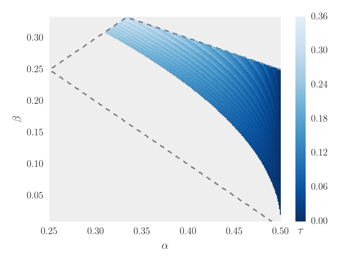
Figure 3: Parametric range in which Kronecker-style models generate dense subgraphs according to the bound derived in Corollary 2. The range in which $\alpha$ is the largest entry of the initiator matrix is circumscribed by the dashed outline. The shading indicates the smallest $\tau$ for which the density $D_{\leqslant\tau k}$ is above one according to the lower bound, gray regions indicate that it lies below one. The banding structure is an artifact of using 20 equally distributed values for $\varepsilon$.

Lemma 8.

For every $0<\tau<1$ it holds that

$$D_{\leqslant\tau k}\geqslant k^{\Theta(1)}\operatorname{\mathbb{E}}[\deg_{\tau k}(x)\mid x\in\mathcal{F}_{\tau k}]$$

with high probability.

Proof.

We have that

$$D_{\leqslant\tau k} =\frac{\|\mathcal{F}_{\leqslant\tau k}\|}{|\mathcal{F}_{\leqslant\tau k}|}\geqslant\frac{|\mathcal{F}_{\tau k}|}{|\mathcal{F}_{\leqslant\tau k}|}\operatorname{\mathbb{E}}[\deg_{\leqslant\tau k}(x)\mid x\in\mathcal{F}_{\tau k}]$$

$$={k\choose\tau k}\Big{(}\sum_{i\leqslant\tau k}{k\choose i}\Big{)}^{-1}\operatorname{\mathbb{E}}[\deg_{\leqslant\tau k}(x)\mid x\in\mathcal{F}_{\tau k}]$$

$$=k^{\Theta(1)}\operatorname{\mathbb{E}}[\deg_{\leqslant\tau k}(x)\mid x\in\mathcal{F}_{\tau k}],$$

and the claim follows from concentration arguments. ∎

It follows that $\operatorname{\mathbb{E}}[\deg_{\tau k}(\cdot)]$ is crucial for the density of graph generated by Kronecker-style models: if there exists a $0<\tau<1$ such that this quantity diverges, then the generated graph contains a dense subgraph with high probability. In particular, such graphs have unbounded degeneracy. We used the family of lower bounds derived in Corollary 2 in order to map out a parametric region that is guaranteed to generate asymptotically dense graphs, cf., Figure 3. As observed above, for $\alpha\geqslant 1/2$ the graphs are necessarily dense and the plot nicely exhibits this trend of very small dense subgraphs as $\alpha$ tends towards $1/2$. Note that in the whole range, the lower bounds for dense subgraphs predict a density that grows like $k^{\Theta(1)}c^{k}$ with $c$ typically around $1.2$. For such moderately exponential functions it is unsurprising that experimental approaches have failed to identify dense subgraphs: for typical ranges of $k$, the polynomial terms easily dominate. Of the undirected graphs listed in Table II, we find that the fitted parameters for AS-Routeviews, Bio-Proteins, and AS-Newman fall into a regime which generates asymptotically dense subgraphs.

IV-B Higher Hamming slices are degenerate

We saw in the previous section that Kronecker-style models often generate asymptotically dense graphs. Our proof located this density in the lower Hamming slices and the question whether the higher slices are sparse arises naturally. Here we show not only that the higher slices are often sparse, we show that they exhibit a sparse structure: if we iteratively remove vertices of low degree, this process will remove all vertices in $\mathcal{F}_{\geqslant\tau k}$, for some fixed $\tau$ depending on the input parameters. We can rephrase this idea in terms of the core-structure of the generated graph as follows:

Lemma 9.

Fix parameters $\bigl{(}\begin{smallmatrix}\alpha&\beta\\ \beta&\delta\end{smallmatrix}\bigr{)},\mu$. Let ${\bar{\tau}}$ be such that for every $\tau\geqslant{\bar{\tau}}$, we have $\operatorname{\mathbb{E}}[\deg_{\leqslant\tau k}(x)\mid x\in\mathcal{F}_{\tau k}]\leqslant 2^{-\Theta(k)}$. Then there exists $c\in\mathbb{R}$ such that the $c$-core of the resulting graphs lies in $\mathcal{F}_{<{\bar{\tau}}k}$ with high probability.

Proof.

Assume $\tau\geqslant{\bar{\tau}}$ and let $x\in\mathcal{F}_{\tau k}$. We apply the multiplicative Chernoff–Hoeffding bound and obtain that

$$\operatorname{\mathbb{P}}[\deg_{\leqslant\tau k}(x)\geqslant c\mu]\leqslant\Big{(}\frac{e}{c\mu}\operatorname{\mathbb{E}}[\deg_{\leqslant\tau k}(x)]\Big{)}^{c\mu}\!\!.$$

Accordingly, the expected number of vertices in $\mathcal{F}_{\tau k}$ with more than $c\mu$ neighbors in $\mathcal{F}_{\leqslant\tau k}$ is at most

$$|\mathcal{F}_{\tau k}|\Big{(}\frac{e}{c\mu}\operatorname{\mathbb{E}}[\deg_{\leqslant\tau k}(x)]\Big{)}^{c\mu}\!\leqslant 2^{k}\Big{(}\frac{e}{c\mu}\operatorname{\mathbb{E}}[\deg_{\leqslant\tau k}(x)]\Big{)}^{c\mu}\!\!.$$

Since $\operatorname{\mathbb{E}}[\deg_{\leqslant\tau k}(x)]=2^{-\Theta(k)}$, we can choose $c$ high enough such that this expected value is upper-bounded by $2^{-k}$ and the claim follows from Markov’s inequality. ∎

Using the upper bounds established in Corollary 3 we can map out what fraction of the higher Hamming slices can be expected to form only sparse connections with higher slices. Figure 4 demonstrates how generator matrices in which $\beta$ is (roughly) at least as large as $\alpha/2$ will result in graphs in which a significant fraction of the vertices fall outside the denser cores. Concerning the networks listed in Table II, we find that the initiator matrices of AS-Routeviews and AS-Newman will generate graphs in which the vertices of $\mathcal{F}_{\geqslant.49k}$ have small degree into higher Hamming slices; for Bio-Proteins the slices $\mathcal{F}_{\geqslant.61k}$, and for Email-Inside the slices $\mathcal{F}_{\geqslant.65k}$.

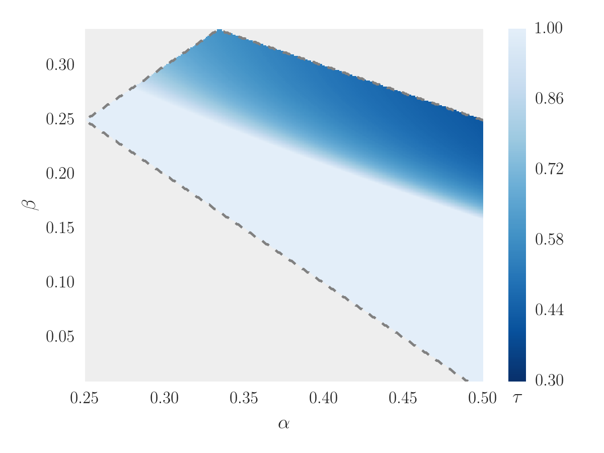
Figure 4: Fraction of Hamming slices $\mathcal{F}_{\geqslant\tau k}$ that fall outside any $c$-core in the sense of Lemma 9 in dependence on the input parameters, determined via the upper bounds provided by Corollary 3. The light area contains those graphs whose core structure does not correlate with the ordering by Hamming weight, in particular Erdős–Rényi graphs at $\alpha=\beta=\delta=0.25$.

V Conclusions

In this paper we obtain two asymptotic results pertaining to the structure of Kronecker-style graph models: (1) a characterization of the conditions under which variants of this model family are asymptotically equivalent, and (2) some members of this family can produce deep core structures and dense subgraphs which are atypical for real-world networks. The latter had not been detected by empirical methods and our asymptotic bounds provide a putative explanation for this fact: the scales at which dense subgraphs and deep cores become apparent lie beyond the usual experimental settings.

In the other extreme, our analysis of the arc probabilities in $\mathrm{SKG}$ and $\mathrm{R\text{-}M\kern-1.00006ptAT}$ led to a statistic that can reveal the difference between these models already at small graph sizes. This calls into question the common approach of treating these models as interchangeable and demands further study.

We conclude that the type of analysis presented here has the capacity to further our understanding of network models beyond currently observable statistics.

References

- [1] J. Leskovec, D. Chakrabarti, J. Kleinberg, and C. Faloutsos, “Realistic, mathematically tractable graph generation and evolution, using Kronecker multiplication,” in Knowledge Discovery in Databases: PKDD 2005. Springer, 2005, pp. 133–145.
- [2] J. Leskovec, D. Chakrabarti, J. Kleinberg, C. Faloutsos, and Z. Ghahramani, “Kronecker graphs: An approach to modeling networks,” The Journal of Machine Learning Research, vol. 11, pp. 985–1042, 2010.
- [3] D. Chakrabarti, Y. Zhan, and C. Faloutsos, “: A recursive model for graph mining.” in SDM, vol. 4. SIAM, 2004, pp. 442–446.
- [4] S. Moreno, S. Kirshner, J. Neville, and S. Vishwanathan, “Tied kronecker product graph models to capture variance in network populations,” in Communication, Control, and Computing (Allerton), 2010 48th Annual Allerton Conference on. IEEE, 2010, pp. 1137–1144.
- [5] C. Seshadhri, A. Pinar, and T. G. Kolda, “An in-depth study of stochastic Kronecker graphs,” in 11th International Conference on Data Mining (ICDM). IEEE, 2011, pp. 587–596.
- [6] S. Todorovic, “Human activities as stochastic Kronecker graphs,” in Computer Vision–ECCV 2012. Springer, 2012, pp. 130–143.
- [7] M. C. Schmidt, N. F. Samatova, K. Thomas, and B. Park, “A scalable, parallel algorithm for maximal clique enumeration,” Journal of Parallel and Distributed Computing, vol. 69, no. 4, pp. 417–428, 2009.
- [8] S. Hill and A. Nagle, “Social network signatures: A framework for re-identification in networked data and experimental results,” in Computational Aspects of Social Networks, 2009. CASON’09. International Conference on. IEEE, 2009, pp. 88–97.
- [9] D. A. Bader and K. Madduri, “A graph-theoretic analysis of the human protein-interaction network using multicore parallel algorithms,” Parallel Computing, vol. 34, no. 11, pp. 627–639, 2008.
- [10] M. Sasaki, L. Zhao, and H. Nagamochi, “Security-aware beacon based network monitoring,” in Communication Systems, 2008. ICCS 2008. 11th IEEE Singapore International Conference on. IEEE, 2008, pp. 527–531.
- [11] J. Leskovec and C. Faloutsos, “Scalable modeling of real graphs using Kronecker multiplication,” in Proceedings of the 24th international conference on Machine learning. ACM, 2007, pp. 497–504.
- [12] C. Groër, B. D. Sullivan, and S. Poole, “A mathematical analysis of the random graph generator,” Networks, vol. 58, no. 3, pp. 159–170, 2011.
- [13] M. Mahdian and Y. Xu, “Stochastic Kronecker graphs,” in Algorithms and models for the web-graph. Springer, 2007, pp. 179–186.
- [14] M. Kang, M. Karoński, C. Koch, and T. Makai, “Properties of stochastic kronecker graphs,” arXiv preprint arXiv:1410.6328, 2014.
- [15] S. Moreno, J. J. Pfeiffer, J. Neville, and S. Kirshner, “A scalable method for exact sampling from Kronecker family models,” in Data Mining (ICDM), 2014 IEEE International Conference on. IEEE, 2014, pp. 440–449.
- [16] A. Pinar, C. Seshadhri, and T. G. Kolda, “The similarity between stochastic Kronecker and Chung–Lu graph models,” in SIAM Conference on Data Mining (SDM12). SIAM, 2012, pp. 1071–1082.
- [17] W. Hoeffding, “Probability inequalities for sums of bounded random variables,” Journal of the American statistical association, vol. 58, no. 301, pp. 13–30, 1963.
- [18] J. Leskovec, K. Lang, A. Dasgupta, and M. Mahoney, “Community structure in large networks: Natural cluster sizes and the absence of large well-defined clusters,” Internet Mathematics, vol. 6, no. 1, pp. 29–123, 2009.
- [19] A. B. Adcock, B. D. Sullivan, and M. W. Mahoney, “Tree-like structure in large social and information networks,” in Proc. of the 2013 IEEE ICDM, 2013, pp. 1–10.
- [20] M. P. Rombach, M. A. Porter, J. H. Fowler, and P. J. Mucha, “Core-periphery structure in networks,” SIAM Journal of Applied Mathematics, vol. 74, pp. 167–190, 2014.
- [21] C. Giatsidis, D. M. Thilikos, and M. Vazirgiannis, “Evaluating cooperation in communities with the k-core structure,” in Advances in Social Networks Analysis and Mining (ASONAM), 2011 International Conference on. IEEE, 2011, pp. 87–93.
- [22] J. I. Alvarez-Hamelin, L. Dall’Asta, A. Barrat, and A. Vespignani, “Large scale networks fingerprinting and visualization using the k-core decomposition,” in Advances in neural information processing systems, 2005, pp. 41–50.
- [23] M. Kitsak, L. K. Gallos, S. Havlin, F. Liljeros, L. Muchnik, H. E. Stanley, and H. A. Makse, “Identification of influential spreaders in complex networks,” Nature physics, vol. 6, no. 11, pp. 888–893, 2010.
- [24] S. Carmi, S. Havlin, S. Kirkpatrick, Y. Shavitt, and E. Shir, “A model of Internet topology using k-shell decomposition,” Proceedings of the National Academy of Sciences, vol. 104, no. 27, pp. 11 150–11 154, 2007.
- [25] J. I. Alvarez-Hamelin, L. Dall’Asta, A. Barrat, A. Vespignani, and et al., “k-core decomposition of Internet graphs: hierarchies, self-similarity and measurement biases,” Networks and Hetereogeneous Media, vol. 3, no. 2, p. 371, 2008.
- [26] V. Batagelj and M. Zaversnik, “An O(m) algorithm for cores decomposition of networks,” arXiv preprint cs/0310049, 2003.
- [27] M. Farrell, T. D. Goodrich, N. Lemons, F. Reidl, F. Sánchez Villaamil, and B. D. Sullivan, “Hyperbolicity, degeneracy, and expansion of random intersection graphs,” in Algorithms and Models for the Web Graph. Springer, 2015, pp. 29–41.
- [28] D. Fernholz and V. Ramachandran, “The giant k-core of a random graph with a specified degree sequence,” 2003. [Online]. Available: http://www.cs.utexas.edu/~vlr/papers/kcore03.pdf
- [29] B. Pittel, J. Spencer, and N. Wormald, “Sudden emergence of a giant -core in a random graph,” Journal of Combinatorial Theory, Series B, vol. 67, no. 1, pp. 111–151, 5 1996.