A new approach for modelling chromospheric evaporation in response to enhanced coronal heating: 1 the method

We present a new computational approach that addresses the difficulty of obtaining the correct interaction between the solar corona and the transition region in response to rapid heating events. In the coupled corona, transition region and chromosphere system, an enhanced downward conductive flux results in an upflow (chromospheric evaporation). However, obtaining the correct upflow generally requires high spatial resolution in order to resolve the transition region. With an unresolved transition region, artificially low coronal densities are obtained because the downward heat flux ‘jumps’ across the unresolved region to the chromosphere, underestimating the upflows. Here, we treat the lower transition region as a discontinuity that responds to changing coronal conditions through the imposition of a jump condition that is derived from an integrated form of energy conservation. To illustrate and benchmark this approach against a fully resolved one-dimensional model, we present field-aligned simulations of coronal loops in response to a range of impulsive (spatially uniform) heating events. We show that our approach leads to a significant improvement in the coronal density evolution than just when using coarse spatial resolutions insufficient to resolve the lower transition region. Our approach compensates for the jumping of the heat flux by imposing a velocity correction that ensures that the energy from the heat flux goes into driving the transition region dynamics, rather than being lost through radiation. Hence, it is possible to obtain improved coronal densities. The advantages of using this approach in both one-dimensional hydrodynamic and three-dimensional magnetohydrodynamic simulations are discussed.

1 Introduction

The interaction between the solar corona and chromosphere is central to understanding the observed properties of magnetically closed coronal loops. It is well known that if the corona is heated impulsively (by for example, a flare, microflare or nanoflare), both the temperature and density increase and then decline, with the time of peak temperature preceding that of the peak density. The changes in density can only be accounted for by mass exchange between the corona and chromosphere, mediated by the transition region (TR).
Recognising the role of the TR is essential for developing reliable models of impulsive heating. For a static equilibrium loop with steady heating, the TR is defined as the region extending from the top of the chromosphere to the location where thermal conduction changes from an energy loss to a gain (e.g. Vesecky et al. 1979). The full TR occupies roughly 10% of the total loop length, the radiation from it is roughly twice that from the corona, and the temperature at its top is of order 60% the temperature at the loop apex (Cargill et al. 2012a). The energy balance in the TR is approximately between downward thermal conduction and optically thin radiation (for a loop in thermal equilibrium).
The change in coronal density in response to impulsive heating arises because the increased coronal temperature implied by the heating gives rise to an excess downward heat flux that the TR is unable to radiate (Klimchuk et al. 2008; Cargill et al. 2012a). The outcome is an enthalpy flux from chromosphere, through the TR, to the corona, often called (chromospheric) ‘evaporation’ (e.g. Antiochos & Sturrock 1978). The location of the TR moves downward in the atmosphere, and the evaporation process actually heats chromospheric material to coronal temperatures. The process is reversed after the density peaks when the TR requires a larger heat flux than the corona can provide, and so instead an enthalpy flux from the corona is set up, which both drains the corona and powers the TR radiative losses (Bradshaw & Cargill 2010a, b). The TR now moves upwards as the chromosphere is replenished.
While straightforward in principle, this heating and upflow followed by cooling and downflow cycle poses major challenges for computational modelling, with conductive cooling being the most severe. For a loop in static equilibrium, in the TR one has an approximate energy equation that equates,

$$\hskip 56.9055pt\kappa_{0}T^{7/2}/L_{T}^{2}\sim(P/2k_{B})^{2}\Lambda(T)/T^{2},$$ (1)

where $L_{T}$ is the temperature length scale (see Eq. (6) for the definition) and the radiative loss function $\Lambda(T)$ decreases as a function of temperature above $10^{5}$K. Thus, one finds $L_{T}^{2}\sim T^{11/2}/\Lambda(T)$, assuming the pressure is constant. Since $T$ decreases in the TR, $L_{T}$ must also decrease rapidly. For a static loop with peak temperature 1.75MK and density 0.25$\times 10^{15}$m^-3, $L_{T}\sim 30$km at $10^{5}$K. When impulsive heating occurs, $L_{T}$ is even smaller. This leads to the familiar difficulty with computational models of loop evolution: how to implement a grid that resolves the TR. Good resolution is essential in order to obtain the correct coronal density (Bradshaw & Cargill 2013, hereafter BC13), otherwise the downward heat flux jumps over an under-resolved TR to the chromosphere where the energy is radiated away. BC13 showed that major errors in the coronal density were likely with lack of resolution.
Since the conductive timescale across a grid point has real physical meaning for the problems at hand, an explicit numerical method is to be preferred (implicit solvers require matrix inversion with no guarantee of convergence). One option is to use brute force on a fixed grid with a large number of grid points. This is slow, since numerical stability of an explicit algorithm requires $\Delta t\leq\textrm{min}(k_{B}n(\Delta z)^{2}/(2\kappa_{0}T^{5/2}))$ (where $\Delta z$ is the cell width and the timestep is the minimum over the whole grid), so that a lot of time is wasted computing in the corona where $L_{T}$ is large and high spatial resolution is not required. A non-uniform fixed grid, with points localised at the TR is an option, but since the TR moves (see above), there is no guarantee that high resolution will be where it is required. Instead, modern schemes use an adaptive mesh which allocates points where they are needed (Betta et al. 1997; Bradshaw & Mason 2003, BC13). The time step restriction is the same as for a uniform grid, but effort is no longer wasted computing highly resolved coronal solutions.
Thus far we have not distinguished between the common one-dimensional (1D) hydrodynamic (field-aligned) modelling and multi-dimensional MHD simulations. It is straightforward for a 1D code with an adaptive mesh and a large computer to model a single heating event, and, with patience, to model a nanoflare train lasting several tens of thousands of seconds (Cargill et al. 2015). However, ensembles of thousands of loop strands heated by nanoflares pose more severe computational challenges. This has led to the development of zero-dimensional field-aligned hydrodynamical models (e.g. Klimchuk et al. 2008; Cargill et al. 2012a, b, 2015) that provide a quick and accurate answer to the coronal response of a loop to heating.
The implementation of field-aligned loop plasma evolution into multi-dimensional MHD models poses much more serious challenges due to the number of grid points that can be used, so that 3D MHD simulations run in a realistic time. This is of the order of $500^{3}$ at the present time. If one desires to resolve the TR with a fixed grid, one needs several thousand points in one direction, so that there will be a loss of resolution elsewhere as well as a potentially crippling reduction of the time step.
The second difficulty is that while an adaptive mesh can still be used in the TR, with commensurate computational benefits, there can be other parts of such simulations that have equally pressing requirements for high resolution, such as current sheets, and, once again, an adaptive mesh does not eliminate the time step problem.
Artificially low coronal densities is the main consequence of not resolving the TR (BC13) and this has significant implications for coronal modelling. The purpose of this paper is to present a physically motivated approach to deal with this problem by using an integrated form of energy conservation that treats the unresolved region of the lower TR (referred to as the unresolved transition region) as a discontinuity, that responds to changing coronal conditions through the imposition of a jump condition.
We describe the key features of the 1D field-aligned model and the definitions used to locate the unresolved transition region (UTR) in Section 2 and Appendix A. The UTR jump condition is derived and the implementation described in Section 3. In Section 4, we present example simulations to benchmark our approach against a fully resolved 1D model. We conclude with a discussion of our new approach and the advantages of employing it, in both 1D and 3D simulations, in Section 5.

2 Equations and numerical method

In this work we model chromospheric evaporation in response to enhanced impulsive coronal heating by considering the 1D field-aligned MHD equations for a single magnetic strand, with uniform cross-section,

$$\frac{\partial\rho}{\partial t}+v\frac{\partial\rho}{\partial z}=-\rho\frac{\partial v}{\partial z},$$ (2)

$$\rho\frac{\partial v}{\partial t}+\rho v\frac{\partial v}{\partial z}=-\frac{\partial P}{\partial z}-\rho g_{\parallel}+\rho\nu\frac{\partial^{2}v}{\partial z^{2}},$$ (3)

$$\rho\frac{\partial\epsilon}{\partial t}+\rho v\frac{\partial\epsilon}{\partial z}=-P\frac{\partial v}{\partial z}-\frac{\partial F_{c}}{\partial z}+Q-\!n^{2}\Lambda(T)\!+\!\rho\nu\!\left(\frac{\partial v}{\partial z}\right)^{\!\!\!2}\!,\!\!$$ (4)

$$P=2\,k_{B}nT.$$ (5)

Here, $z$ is the spatial coordinate along the magnetic field, $\rho$ is the mass density, $P$ is the gas pressure, $T$ is the temperature, $k_{B}$ is the Boltzmann constant, $\epsilon=P/(\gamma-1)\rho$ is the specific internal energy density, $n$ is the number density ($n=\rho/1.2m_{p}$, $m_{p}$ is the proton mass), $v$ is the velocity parallel to the magnetic field, $g_{\parallel}$ is the field-aligned gravitational acceleration (for which we use a profile that corresponds to a semi-circular strand), $\nu$ is the viscosity (shock viscosity is also included as discussed in Arber et al. (2001)), $F_{c}=-\kappa_{0}T^{5/2}\partial T/\partial z$ is the heat flux, $Q$ is the volumetric heating rate and $\Lambda(T)$ is the optically thin radiative loss function for which we use the piecewise continuous form defined in Klimchuk et al. (2008).
We solve the 1D field-aligned MHD equations using two different methods, a Lagrangian remap (Lare) approach, as described for 3D MHD in Arber et al. (2001), adapted for 1D field-aligned hydrodynamics (Lare1D) and the adaptive mesh code HYDRAD (Bradshaw & Mason 2003). Time-splitting methods are used in Lare to update thermal conduction and optically thin radiation separately from the advection terms, as discussed in Appendix A. Furthermore, to treat thermal conduction we use super time stepping (STS) methods, as described in Meyer et al. (2012, 2014) and discussed in Appendix B.

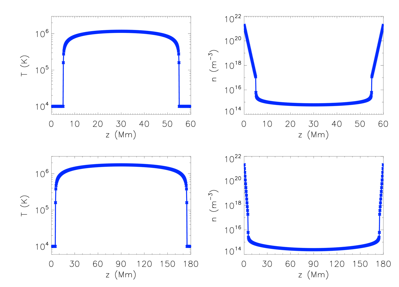
Figure 1: Temperature and density initial conditions with 500 grid points along the length of the loop. Upper panels: $60$Mm loop with $Q_{bg}=2.2167\times 10^{-5}$Jm^-3s^-1. Lower panels: $180$Mm loop with $Q_{bg}=6.8682\times 10^{-6}$Jm^-3s^-1. Each asterisk represents a single grid point.

The initial condition of the model is a magnetic strand (loop) in static equilibrium. This is obtained by starting with an extremely high resolution uniform grid with $5\times 10^{5}$ grid points along the length of the loop. We consider both a short (60Mm) and long (180Mm) loop, where the total length of each loop (2L) includes a 5Mm model chromosphere (included as a mass reservoir) at the base of each TR ($z=5$Mm). We set $T=10,000$K and n=$10^{17}$m^-3 at the base of the TR. The initial equilibrium temperature and density profiles are then derived using the same approach as described in Bradshaw & Mason (2003). We note that, to achieve thermal balance, a small background heating term is necessary ($Q_{bg}$). These fully resolved equilibrium solutions are then interpolated onto the much coarser grids used for the time-dependent evolution. The initial conditions, with 500 grid points along the length of the loop, are shown for both the short and long loop in Fig. 1. We note that neither solution is numerically resolved below approximately $2\times 10^{5}$K until the chromospheric temperature is reached.

2.1 Definitions

We use coarse spatial resolutions and address the influence of poor numerical resolution by modelling the unresolved region of the atmosphere, which we refer to as the UTR, as a discontinuity by using an appropriate jump condition, instead of trying to implement a grid that fully resolves the TR. To facilitate the formulation of this approach, we first introduce some definitions. We define the temperature length scale as,

$$\hskip 56.9055ptL_{T}=\frac{T}{|dT/dz|}=\frac{\kappa_{0}T^{7/2}}{|F_{c}|}.$$ (6)

With a uniform grid, the resolution in the simulation is given by,

$$\hskip 85.35826ptL_{R}=\frac{2L}{N_{z}-1},$$ (7)

where $N_{z}$ is the number of grid points along the length of the loop (2L). (A non-uniform grid will have the same problems, amenable with a similar solution.) Using these definitions, we define the top of the UTR ($z_{0}$) to be the final location, when moving downwards from the loop apex ($z_{a}$), at which the criteria,

$$\hskip 85.35826pt\frac{L_{R}}{L_{T}}\leq\delta<1,$$ (8)

is satisfied. To ensure that we have sufficient resolution at the top of this region, that is multiple grid points across the temperature length scale, we take $\delta=1/4$ throughout this paper.
Fig. 2 demonstrates the consequences of Eq. (8) for short (long) loops in the upper (lower) panel. The product of $\delta$ and $L_{T}$ is shown as a function of temperature (solid blue line) with the red dashed lines showing different values of $L_{R}$. Any temperature that falls below the dashed lines will be part of an UTR. This arises below a few $10^{5}$K. Also when coarse resolution is used, the temperature at the top of the UTR is only weakly dependent on the spatial resolution.
Lastly, we define the base of the TR ($z_{b}$) to be the location at which the temperature first reaches or falls below the chromospheric temperature (10,000K). Employing these definitions it is straightforward to locate both the top of the UTR and the base of the TR at all time steps during a simulation.

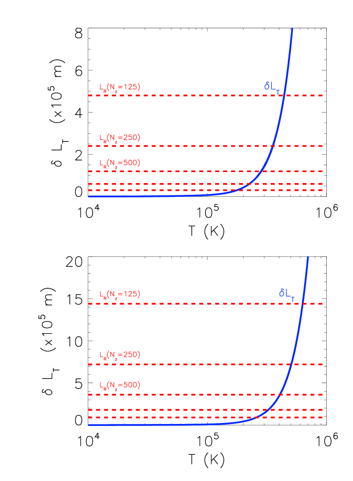
Figure 2: The product of $\delta$ and the temperature length scale ($L_{T}$) as a function of temperature (solid blue line) based on fully resolved equilibrium solutions that are computed with $5\times 10^{5}$ grid points along the length of the loop and are consistent with the short and long loop initial conditions shown in Fig. 1. Upper panel: $60$Mm loop. Lower panel: $180$Mm loop. The dashed red lines are the simulation resolutions ($L_{R}$) obtained by using different numbers of grid points. In both plots, starting from the top the first dashed red line corresponds to 125 grid points, the second to 250 grid points, the third to 500 grid points, the fourth to 1,000 grid points and the fifth to 2,000 grid points.

3 Unresolved transition region jump condition

On use of equations (2)–(4), one can write an equation for the total energy in conservative form,

$$\frac{\partial E}{\partial t}=-\frac{\partial}{\partial z}(Ev+Pv+F_{c})+Q-n^{2}\Lambda(T),$$ (9)

where the total energy is the sum of thermal, kinetic and gravitational potential energy,

$$\hskip 56.9055ptE=\frac{P}{\gamma-1}+\frac{1}{2}\rho v^{2}+\rho\Phi.$$ (10)

Here, $\Phi$ is the gravitational potential ($g_{\parallel}=d\Phi/dz$).
We integrate Eq. (9) over the UTR (of length $\ell$), from the base of the TR ($z_{b}$) upwards to the top of the UTR ($z_{0}$), to obtain,

$$\ell\frac{d\bar{E}}{dt}= -E_{0}v_{0}-P_{0}v_{0}-F_{c,0}$$

$$+E_{b}v_{b}+P_{b}v_{b}+F_{c,b}+\ell\bar{Q}-\mathcal{R}_{utr},$$ (11)

where the subscripts 0 and b indicate quantities evaluated at the top and base of the UTR, respectively. The overbars indicate spatial averages over the UTR and $\mathcal{R}_{utr}$ is the integrated radiative losses (IRL) in the UTR (see Eq. (13) for the definition).
Using the fully resolved HYDRAD results, we have confirmed that $F_{c,b}$ is always small ($F_{c,b}<<F_{c,0}$) and that after the intial downward motion of the TR (during the heating phase), the terms containing $v_{b}$ are also significantly smaller than the remaining terms on the right-hand side (RHS) of Eq. (11). It is these remaining terms that control the coronal response. Hence, we follow Cargill et al. (2012a) and neglect these terms from now on.
We have also confirmed, from the fully resolved results, that there are only short intervals (at the start of the heating period) when $\ell d\bar{E}/dt$ can be significant. However, the problem with including this term is that, with the resolution of current 3D MHD models, it is very difficult to calculate $\ell d\bar{E}/dt$ accurately because the calculation requires $dE/dt$ to be integrated across the UTR. If the TR is not fully resolved then the heat flux jumps across the UTR, resulting in the estimates of $dE/dt$ being in error. Indeed, if we could calculate $\ell d\bar{E}/dt$ accurately, with coarse spatial resolutions, then it would not be necessary to implement a method to obtain the correct upflow and evaporation. Therefore, the final assumption in the derivation of our jump condition is to adopt the approach of Klimchuk et al. (2008) and neglect the left-hand side (LHS) of Eq. (11).
Under these assumptions, by combining equations (10) & (11), we obtain the jump condition at the top of the UTR,

$$\frac{\gamma}{\gamma-1}P_{0}v_{0}+\frac{1}{2}\rho_{0}v_{0}^{3}+\rho_{0}\Phi_{0}v_{0}=-F_{c,0}+\ell\bar{Q}-\mathcal{R}_{utr},$$ (12)

where

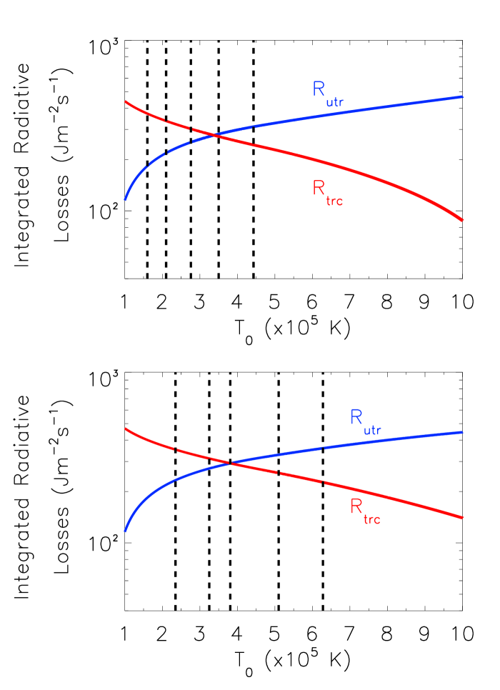
Figure 3: IRL in the UTR (solid blue line) and resolved upper TR and corona (solid red line) based on fully resolved equilibrium solutions that are computed with $5\times 10^{5}$ grid points along the length of the loop and are consistent with the short and long loop initial conditions shown in Fig. 1. Upper panel: $60$Mm loop. Lower panel: $180$Mm loop. The dashed black lines are the temperatures at the top of the UTR ($T_{0}$) that are obtained by using the different simulation resolutions ($L_{R}$). In both plots, starting from the right the first dashed black line corresponds to 125 grid points, the second to 250 grid points, the third to 500 grid points, the fourth to 1,000 grid points and the fifth to 2,000 grid points.

the terms on the LHS are the enthalpy flux ($F_{e}$), kinetic energy flux and gravitational potential energy flux, respectively. The terms on the RHS are the heat flux, the average volumetric heating rate per unit cross-sectional area and the IRL in the UTR respectively. We refer to Eq. (12) as the UTR jump condition and propose that the UTR should be modelled as a discontinuity using Eq. (12) to impose a corrected velocity ($v_{0}$) at the top of the UTR, at each time step.
This corrected velocity is imposed following the conduction and radiation and heating steps, prior to the advection step, as illustrated in Fig. 10, while the flow at the base of the TR $(v_{b})$ is subsequently accounted for during the advection step. Consequently, at the time of calculation of $v_{0}$, it is possible to calculate the heat flux ($F_{c,0}$) and the average volumetric heating rate per unit cross-sectional area in the UTR ($\ell\bar{Q}$). Of the terms on the LHS of the UTR jump condition (12), the pressure ($P_{0}$), density ($\rho_{0}$), and gravitational potential ($\Phi_{0}$) are also known. The main challenge is the calculation of the IRL in the UTR ($\mathcal{R}_{utr}$).

Table 1: A summary of the parameter space used and results from the numerical simulations.

Case	2L	$Q_{H}$	$\tau_{H}$	$T_{\textrm{max}}(\textrm{HYDRAD})$	$T_{\textrm{max}}(\textrm{LareJ})$	$T_{\textrm{max}}(\textrm{Lare1D(500)})$	$n_{\textrm{max}}(\textrm{HYDRAD})$	$n_{\textrm{max}}(\textrm{LareJ})$	$n_{\textrm{max}}(\textrm{Lare1D(500)})$
	(Mm)	(Jm-3s-1)	(s)	(MK)	(MK)	(MK)	($10^{15}$m-3)	($10^{15}$m-3)	($10^{15}$m-3)
1	60	$8\times 10^{-4}$	60	1.9	2.1	2.1	0.86	0.92	0.74
2	60	$8\times 10^{-3}$	60	5.7	6.1	6.1	2.2	2.6	1.5
3	60	$8\times 10^{-2}$	60	12.5	12.9	13.1	9.0	11.6	4.9
4	60	$8\times 10^{-4}$	600	3.4	3.5	3.5	2.2	2.6	1.0
5	60	$8\times 10^{-3}$	600	6.9	7.1	6.9	9.1	11.4	2.9
6	60	$8\times 10^{-2}$	600	13.7	14.1	13.8	40.3	49.7	10.4
7	180	$5\times 10^{-5}$	60	1.8	1.8	1.8	0.28	0.29	0.27
8	180	$5\times 10^{-4}$	60	2.9	3.1	3.1	0.37	0.40	0.33
9	180	$5\times 10^{-3}$	60	9.3	10.2	10.2	1.0	1.13	0.42
10	180	$5\times 10^{-5}$	600	2.5	2.7	2.7	0.36	0.40	0.33
11	180	$5\times 10^{-4}$	600	5.7	6.0	6.0	0.98	1.18	0.39
12	180	$5\times 10^{-3}$	600	12.3	12.7	12.3	4.2	5.4	1.2

3.1 Integrated radiative losses in the unresolved transition region

Motivated by equilibrium results, we estimate $\mathcal{R}_{utr}$ using the IRL in the resolved upper TR and corona ($\mathcal{R}_{trc}$),

$$\hskip 56.9055pt\mathcal{R}_{utr}=\int_{z_{b}}^{z_{0}}\!\!\!\!n^{2}\Lambda(T)\,dz\approx\mathcal{R}_{trc},$$ (13)

where,

$$\hskip 56.9055pt\mathcal{R}_{trc}=\int^{z_{{a}}}_{z_{0}}\!\!\!\!n^{2}\Lambda(T)\,dz.$$ (14)

To demonstrate the justification of (13), in Fig. 3 we plot the IRL in the UTR ($\mathcal{R}_{utr}$) and resolved upper TR and corona ($\mathcal{R}_{trc}$) as functions of the temperature at the top of the UTR ($T_{0}$), for both our short and long loop initial conditions. These curves are obtained by integrating the radiative losses from fully resolved solutions (using $5\times 10^{5}$ uniformly spaced grid points) while adjusting the integration limits so that the spatial location of the top of the UTR changes with the temperature at this location. Previously, we have seen that when coarse resolution is used, the temperature at the top of the UTR is only weakly dependent on the spatial resolution (see Fig. 2), which means that there is only a small range of resolvable TR temperatures before the unresolved region of the atmosphere is reached, and within these small temperature ranges there is reasonably good agreement between the values of $\mathcal{R}_{trc}$ and $\mathcal{R}_{utr}$. For example, as can be seen in Fig. 3, when using 1,000 grid points with $2L=180$Mm, $T_{0}=3.25\times 10^{5}$K and $\mathcal{R}_{utr}\,(272$Jm^-2s${}^{-1})$ $\approx$ $\mathcal{R}_{trc}\,(312$Jm^-2s${}^{-1})$. We note that the agreement is even better when using 500 grid points.
But when coarse resolution is used, a single grid point lower down in the atmosphere can have a considerable effect on the IRL in the resolved upper TR and corona. Therefore, we note that it is safer to define the top of the UTR to be a few grid cells higher up than previously defined.

3.2 Implementation of the jump condition

Once the IRL in the UTR ($\mathcal{R}_{utr}$) have been estimated, the corrected velocity ($v_{0}$) is then calculated, by firstly solving the UTR jump condition (12), which is a cubic in $v_{0}$, using a simple Newton-Raphson solver with the starting condition,

$$\hskip 56.9055ptv_{i}=\dfrac{-F_{c,0}+\ell\bar{Q}-\mathcal{R}_{utr}}{(\gamma-1)/\gamma P_{0}},$$ (15)

which is obtained by neglecting the kinetic energy and gravitational potential energy fluxes in Eq. (12). Convergence to a solution of the complete equation is rapid.
In some cases approximation (13) underestimates the IRL in the UTR, which may lead to spurious supersonic upflows for the class of problems considered in this paper. Therefore, the solution to Eq. (12), $\tilde{v}_{0}$, is adjusted by using the following sound speed limiter,

$$\hskip 85.35826ptv_{0}=\dfrac{\quad\tilde{v}_{0}\times c_{s}}{\sqrt{\tilde{v}_{0}^{2}+c_{s}^{2}}},$$ (16)

where $c_{s}$ is the local sound speed at the top of the UTR. It is this adjusted velocity ($v_{0}$) that we impose at the top of the UTR. This is consistent with the corresponding fully resolved loop simulations (that use an adaptive mesh), since no supersonic flows are present at the location where the jump condition is implemented, in all of the 12 cases considered. Hence, this approximation is satisfactory for the problems presented here and it does not inhibit the existence of supersonic flows higher up in the atmosphere.

Table 2: Numerical simulation computation times.

Case	$\tau(\textrm{\scriptsize LareJ})$	$\tau(\textrm{\scriptsize HYDRAD})$	$\tau(\textrm{\scriptsize Lare1D(8,000)})$	$\tau(\textrm{\scriptsize HYDRAD})/$	$\tau(\textrm{\scriptsize Lare1D(8,000)})/$
	(mins)	(mins)	(mins)	$\tau(\textrm{\scriptsize LareJ})$	$\tau(\textrm{\scriptsize LareJ})$
1	17	316	7,426	18.6	436.8
2	19	340	7,766	17.9	408.7
3	51	1,943	13,886	38.1	272.3
4	22	370	6,341	16.8	288.2
5	82	2,617	8,594*	31.9	106.0
6	154	5,177	12,732*	33.6	82.7
7	26	1,559	18,893	60.0	726.7
8	28	1,566	18,059	56.0	645.0
9	35	1,605	16,833	45.9	480.9
10	26	1,805	11,138	69.4	428.4
11	32	1,914	11,997	59.8	374.9
12	86	2,269	12,973*	26.4	150.8

Figure 4: Results for Case 9. The panels show the coronal averaged temperature, density and pressure as functions of time, and the temperature versus density phase space plot. The solid lines represent the Lare1D solutions obtained by using different numbers of grid points along the length of the loop, the dashed blue line is the LareJ solution (that is computed with the same spatial resolution as the solid blue curve) and the dot-dashed orange line corresponds to the HYDRAD solution.

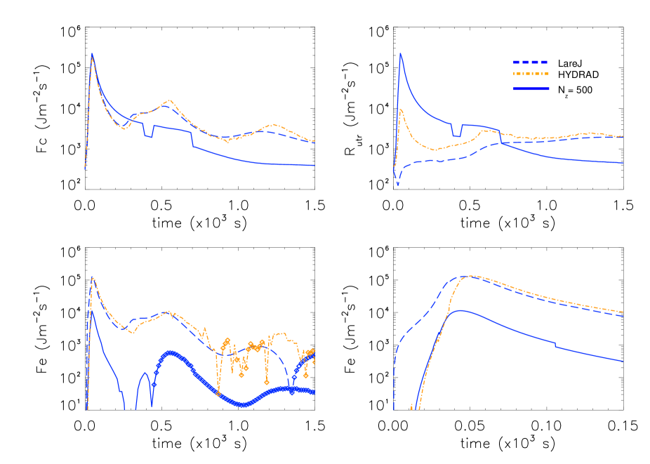
Figure 5: Results for Case 9. The panels show the heat flux at the top of UTR, IRL in the UTR and enthalpy flux over two different time intervals at the top of the UTR (lines connected by diamond symbols indicate where the enthalpy flux is downflowing and lines without diamonds indicate where the enthalpy flux is upflowing) as functions of time. The dashed blue line is the LareJ solution (that is computed with 500 grid points along the length of the loop), the solid blue line is the Lare1D solution that is computed with 500 grid points along the length of the loop and the dot-dashed orange line corresponds to the HYDRAD solution.

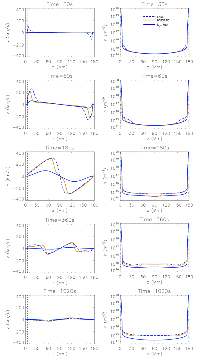
Figure 6: Results for Case 9. The panels show the velocity and density as functions of position for times during the evaporation phase up until the second density peak. The dashed blue line is the LareJ solution (that is computed with 500 grid points along the length of the loop), the solid blue line is the Lare1D solution that is computed with 500 grid points along the length of the loop and the solid orange line corresponds to the HYDRAD solution. The dashed black line indicates the position of the top of the UTR ($z_{0}$)

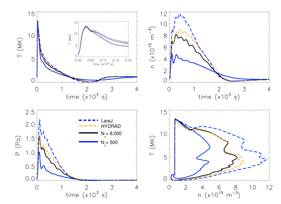
Figure 7: Results for Case 3. Notation is the same as Fig. 4 but note the different time axis.

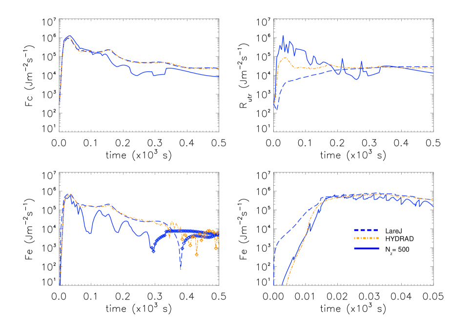
Figure 8: Results for Case 3. Notation is the same as Fig. 5 but note the different time axis.

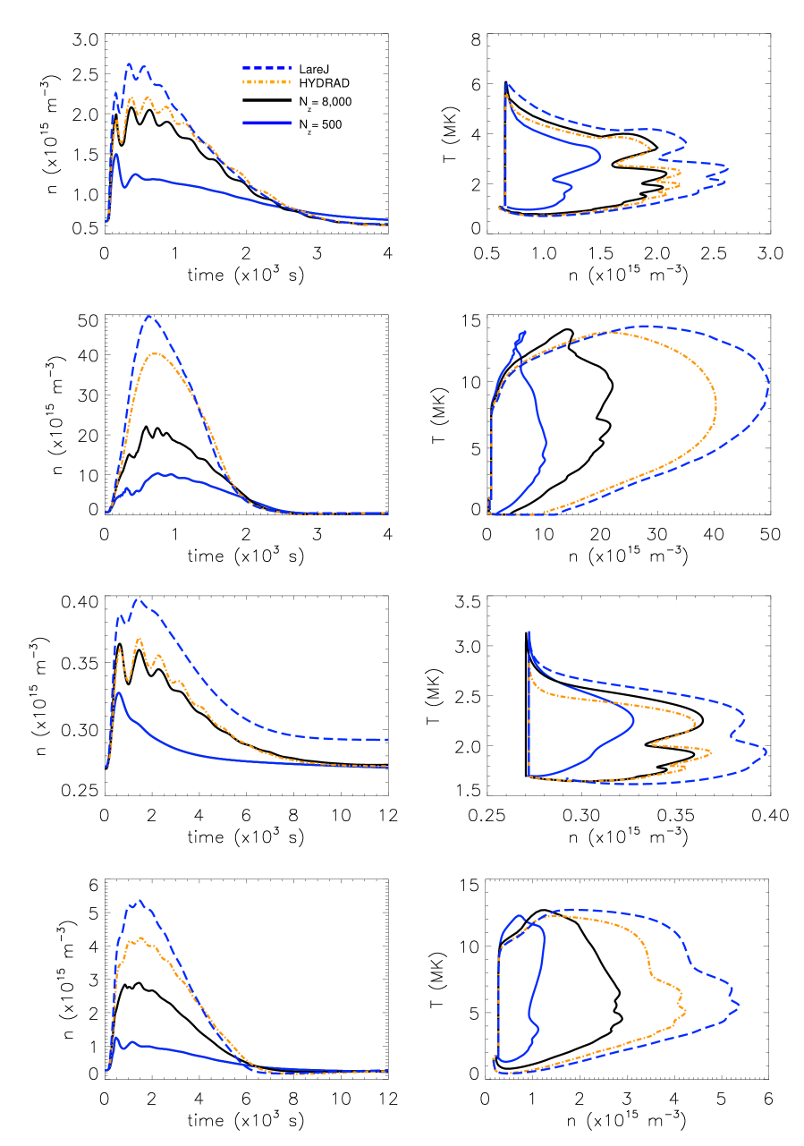
Figure 9: Results for Cases 2 (upper two panels), 6 (upper central two panels), 8 (lower central two panels) and 12 (lower two panels). The panels show the coronal averaged density as a function of time and the temperature versus density phase space plot.

4 Results

The effectiveness of the UTR jump condition to obtain a physically realistic evolution, through the complete coronal heating and cooling cycle, when employed with coarse resolution is investigated for a series of impulsive coronal heating events. The heating events considered are based on the cases (1-12) that were previously studied in BC13. These events are described in Table 1 and cover several orders of magnitude and duration of heating for both a short and long loop. The energy release is also the same as that used in BC13. The temporal profile is triangular with a peak value of $Q_{H}$ and total duration of $\tau_{H}$ while the spatial profile is uniform along the loop.
For each case, the main assessment of the performance of the UTR jump condition model is a comparison of Lare1D using 500 grid points employed with the jump condition (referred to as LareJ), with both Lare1D without the jump condition but using up to 8,000 grid points and the adaptive mesh code HYDRAD. The choice of 500 grid points is motivated by what is routinely used in current multi-dimensional MHD models (Bourdin et al. 2013; Hansteen et al. 2015; Hood et al. 2016; Dahlburg et al. 2016). The spatial resolution of these solutions is $120$km and $360$km for the short and long loop, respectively.
For the Lare1D solutions we employ a uniform grid and repeat each run with $N_{z}=[500,\,1,000,\,2,000,\,4,000,\,8,000]$ grid points along the length of the loop. We note that because we are using a uniform grid each time we double the number of grid points, even although we improve the TR resolution, we also further reduce the thermal conduction timescale in the corona and so the computational time increases. Therefore, we have limited the most refined resolution used here because of the increased computation time required.
Consistent with our model equations (2)-(5), we run the HYDRAD code in single fluid mode. The HYDRAD code has an adaptive grid that is capable of increasing the numerical resolution wherever it is needed based on selected refinement conditions. This enables the code to fully resolve the small length scales in the TR while retaining a coarser grid elsewhere. Following BC13, we select the largest grid cell to be of width $400$km and employ 12 levels of refinement, so that in the most highly resolved regions the grid cells are of width $98$m. In this paper, we assume that the HYDRAD solution is ‘correct’ .

4.1 Case 9

BC13 found their Case 9 (a strong nanoflare in a long loop) to be one of the more challenging examples for obtaining correct coronal densities. Fig. 4 shows the temporal evolution of the coronal averaged temperature ($T$), density ($n$), pressure ($P$) and the corresponding temperature versus density phase space plot. The coronal averages are computed by spatially averaging over the uppermost 50% of the loop. (The trends are the same if either the averages are computed over the full portion of the loop above $z_{0}$ or the values are compared at the top of the UTR.) In the plots each solid line corresponds to a Lare1D solution that was calculated by employing a different number of grid points along the length of the loop. The solid blue line has 500 grid points ($L_{R}\!=\!360$km), the green line has 1,000 grid points ($L_{R}\!=\!180$km), the red line has 2,000 grid points ($L_{R}\!=\!90$km), the purple line has 4,000 grid points ($L_{R}\!=\!45$km) and the black line has 8,000 grid points ($L_{R}\!=\!22.5$km). The dashed blue line is the LareJ solution that is computed with 500 grid points along the length of the loop and the dot-dashed orange line corresponds to the HYDRAD solution.
Starting with the Lare1D solutions it is clear that we recover the result presented by BC13, namely that the main effect of insufficient resolution is on the coronal density while the temperature is far less resolution dependent. We also note that in this case, as is predicted by BC13 the most refined resolution that we employed with the Lare1D code is still not capable of reproducing the fully resolved HYDRAD solution.
However, if we focus on the LareJ solution, there is good agreement between the LareJ and HYDRAD solutions. At the initial density peak, the LareJ solution evaporates about 10% too much material upwards into the corona, in comparison to the HYDRAD solution, while the density of the corresponding coarse Lare1D solution (run with the same spatial resolution, solid blue line) is more than a factor of two lower than the resolved loop value. As a consequence of this difference in densities, because the conductive cooling timescale scales as $n/T^{5/2}$, the LareJ solution cools at the correct rate while there is evidence that the corresponding coarse Lare1D solution cools more rapidly.
The density then oscillates as the plasma sloshes to and fro within the loop. These oscillations are captured to a large extent by the LareJ solution but are not prominent in the corresponding coarse Lare1D solution. During these oscillations, even although the LareJ density remains slightly too high, the accuracy of the LareJ solution is still an improvement on even the most refined Lare1D solution. The LareJ solution then goes on to attain the correct draining rate during the density decay phase before recovering the equilibrium.
Bringing all these factors together, in the phase space plot it is evident that the LareJ solution captures the evolution of the density as a function of temperature more accurately than the entire set of Lare1D solutions, including the most refined solution that has a factor of 16 more grid points along the length of the loop.
Table 2 summarises the CPU requirements for all cases and demonstrates the large gain in CPU time of the UTR jump condition method over the HYDRAD and most refined Lare1D runs. Therefore, in this particular case, our method obtains a coronal density comparable to HYDRAD (fully-resolved 1D model) but with a significantly faster computation time and also provides a significant improvement in the accuracy of the coronal density evolution when compared to the equivalent simulations run without the jump condition.
Using HYDRAD, BC13 demonstrated that, for reasonably accurate solutions in the case of 180Mm loops and peak temperatures exceeding 6MK, cell widths of no more than 5km are required. What we have shown in Fig. 4 - 6 is that it is possible to obtain realistic densities, temperatures and velocities with cell widths of 360km by using the UTR jump condition employed in LareJ.
We now turn our attention to understanding why the LareJ solution performs well for this particular heating event (Case 9). Fig. 5 shows the temporal evolution of the heat and enthalpy fluxes at the top of the UTR and the IRL in the UTR. These quantities are the dominant terms in the UTR jump condition (12) although the loop’s evolution can be influenced by the additional terms in Eq. (12) that are not shown here. The dashed blue lines represent the appropriate LareJ quantities and the dot-dashed orange (solid blue) lines represent the appropriate quantities that are obtained throughout the evolution of the HYDRAD solution (Lare1D solution computed with 500 grid points along the length of the loop) . To calculate these quantities the definition of the UTR is determined based on the time evolution of the temperature from the LareJ solution.
During the initial evaporation phase (first 400s) the excess heat flux drives an upward enthalpy flux. Throughout this phase there is good agreement between the enthalpy fluxes of the LareJ and HYDRAD solutions. This agreement is achieved because the downward heat flux dominates the IRL in the UTR and so the UTR jump condition principally returns the heat flux as an upward enthalpy flux.
However, close inspection reveals that, throughout the first 40s (see lower right panel in Fig. 5), the enthalpy flux of the LareJ solution exceeds that of the HYDRAD solution. During this period the LareJ radiation approximation (13) is least accurate and leads to an underestimation of the IRL in the UTR. It is this underestimation of the IRL that drives the enhanced enthalpy flux.
Fig. 6 shows the velocity and density as functions of position, from the LareJ, coarse Lare1D and HYDRAD simulations, for times during the evaporation phase up until the second density peak. The enhanced enthalpy flux, throughout the first 40s, indicates that the correcting velocity ($v_{0}$), imposed at the top of the UTR, is overestimated during this period. This is confirmed in the top left panel in Fig. 6. Therefore, the underestimation of the IRL in the UTR leads to an overestimation in the initial upflow, locally at the top of the UTR, which then generates an enhanced global velocity that facilitates the over evaporation of the LareJ solution.
Despite this overestimation in the initial upflow, by imposing the correcting velocity ($v_{0}$) locally at the top of UTR, the jump condition method is still able to capture the global velocity much more accurately, in time, than the corresponding simulation run without the jump condition (see Fig. 6).
Radiation becomes increasingly important as the density increases. Then, at the time when the radiation finally exceeds the heat flux, the loop enters the density decay phase because a downward enthalpy flux (condensation) is required to power the TR radiation. During this decay phase, the LareJ solution drains material from the corona at the correct rate due to the improvement in the accuracy of the LareJ radiation estimation (13), following the first density peak.

4.2 Case 3

BC13 found their Case 3 (a small flare in a short loop) demanded the most severe requirements on the spatial resolution. Grid cells of width 390m were needed, in the most refined regions, in order for the coronal density to exceed 90% of the properly resolved value. The results for the numerical simulations included in this case are shown in Fig. 7 and 8. To show the comparison exclusively between the key solutions, in the coronal averaged plots, we now drop the intermediate Lare1D solutions.
In this particular case, even although the LareJ solution suffers from its most significant over evaporation at the initial density peak (about 30%) and the density remains too high throughout the first 1,000s, its performance remains reasonably encouraging from the viewpoint that the LareJ solution follows the same fundamental evolution as the HYDRAD solution and their agreement is good throughout the density decay phase. The factors responsible for driving this behaviour in the LareJ solution are the same as those seen previously in Case 9.

4.3 Remaining cases

We present the numerical comparison for the remaining cases in Table 1, where the maximum averaged coronal temperature and density attained by the HYDRAD, LareJ and corresponding coarse Lare1D solutions are shown. In all 12 cases, the table shows that the accuracy of the maximum coronal density is considerably improved with the LareJ solution when compared to the same resolution run without the jump condition implemented.
The results for the Cases 2, 6, 8 and 12 are shown in Fig. 9. Essentially, because we drive the temperature throughout the impulsive heating event, we have seen that the temporal evolution of the coronal averaged temperature is only weakly dependent on both the spatial resolution and computational method used. Therefore, it is sufficient to now show only the temporal evolution of the coronal averaged density and the corresponding temperature versus density phase space plots.
In these cases, the UTR jump condition method consistently captures a physically realistic evolution, through the complete coronal heating and cooling cycle, comparable to that of the HYDRAD solutions. The estimation of the IRL in the UTR is again identified as the main source of error that drives the observed over evaporation. This is due to the simple radiation estimation (13) used and despite this, it remains clear that as a first approximation, the LareJ solutions are reasonably good, providing a significant improvement on the corresponding coarse simulations run without the jump condition.
However, we note from the phase space plot of Case 8 that (1) for this particular heating event, the most refined Lare1D solution (the black line, computed with 8,000 grid points) has a much better agreement with HYDRAD than the LareJ solution and (2) the LareJ solution does not recover the exact long loop initial equilibrium, but returns to another nearby equilibrium with an increased density of around 7% (similar behaviour was also seen in BC13). This is true for all of the long loop cases considered but is only observable in those where the density increase, in response to the heating event, is small (e.g. Cases 7 & 8).

5 Discussion and conclusions

The difficulty of obtaining adequate spatial resolution in numerical simulations of the corona, transition region (TR) and chromosphere system has been a long-standing problem. As pointed out by BC13, the main consequence of not resolving the TR is that the resulting coronal density is artificially low. This paper has presented an approach to deal with this problem by using an integrated form of energy conservation that essentially treats the lower TR as a discontinuity. Hence, the response of the TR to changing coronal conditions is determined through the imposition of a jump condition. When compared to fully resolved 1D models (e.g. BC13), our new approach generated improved coronal densities with significantly faster computation times than the corresponding high-resolution and fully resolved models. Specifically, our approach required at least one to two orders of magnitude less computational time than fully resolved (high-resolution) models.
The 12 cases presented in this paper were selected to correspond to the benchmark cases presented by BC13. In all 12 cases, the evolution of the coronal density is considerably improved, compared to the same resolution run without the jump condition implemented. Crucial here, is to obtain a reasonable estimate of the (integrated) radiative losses in the unresolved part of the TR.
We have considered only spatially uniform impulsive heating events. Simulations with the heating concentrated either at the loop base or near the loop apex will be presented in a subsequent publication.
The advantages of this new approach are multiple. For 1D hydrodynamic simulations of the coronal response to heating (see e.g. Reale 2014, for a review), the short computation time means that (a) simulations of coronal heating events can be run quickly, permitting an extensive survey of the (large) parameter space and (b) simulations of multiple loop strands (thousands or more) that either comprise a single observed loop (e.g. a core loop), or an entire active region, can be performed with relative ease. In 3D MHD codes, the method can be included without the need for higher spatial resolution and a corresponding extended computation time. Indeed, our results suggest that good accuracy can be obtained with the order of 500 grid points, typical of what is routinely used in current 3D MHD simulations. The extension to 3D will be addressed fully in a future publication.
The work presented here has adopted the simplest possible model for the radiation in the lower, unresolved transition region (UTR), and leads to improved coronal densities. The estimate used was motivated by the calculation of the radiation integrals for the equilibrium conditions (as shown in Fig. 3), at which the error is at most around a factor of 2 when using a uniform grid with between 125 and 2,000 grid points. On the other hand, the densities are systematically higher than those in fully resolved 1D models, which can be tracked down to the simple model underestimating the true value of the integrated radiative losses in the UTR ($R_{utr}$), at the very start of the heating phase. One can mitigate this problem by using slightly more complicated models for $R_{utr}$ at the start of the increased heating event and this will be addressed in a subsequent publication. However, for the present, the density draining phase is captured correctly which is important as this is the phase that is seen in many observations of coronal loops. We note that in Case 8, during this phase and throughout the entire evolution, the most refined uniform grid solution (Lare1D with 8,000 grid points) achieved a better agreement with the fully resolved model than the jump condition (LareJ with 500 grid points) solution but at significantly greater computational cost.
Our emphasis here has been on obtaining an improved coronal density. This is important for interpreting observations of, for example, active region loop cores, ‘warm’ loops, as well as microflare and flare coronal emission. On the other hand, by treating the lower (unresolved) TR as a discontinuity, information will be lost on detailed TR emission lines such as CIV. If the jump condition is applied close to 1 MK (i.e. between $5\times 10^{5}$ K and 1 MK) the details of the (bright) TR will be lost, although integrated TR quantities can of course still be deduced. This loss of detail would particularly affect studies of, for example, the bright TR “moss” – bright emission at the footpoints of very hot loops (see e.g. Fletcher & De Pontieu 1999). Full numerical resolution is still required to deduce these, with the corresponding risk of serious errors in the plasma density. Model setups with smaller coronal domains (coronal heights) and or lower temperatures (say below 1-2 MK) are likely to have adequate resolution (e.g. Zacharias et al. 2011; Hansteen et al. 2015).
In summary, this paper has presented an approach to deal with the difficulty of obtaining the correct interaction between a downward conductive flux from the corona and the resulting upflow from the TR. A wide range of impulsive (spatially uniform) heating events was considered for both short and long loops. Our new method was used in simulations with coarse resolutions that do not resolve the lower transition region. The main result is that the method leads to (i) coronal densities comparable to fully-resolved 1D models but with significantly faster computation times, and (ii) significant improvements in the accuracy of both the coronal density and temperature temporal evolution when compared to the equivalent simulations run without this approach.

Appendix A Lare1D with thermal conduction and radiation

The 1D field-aligned MHD equations (2)-(5) are solved using a Lagrangian remap (Lare) approach, as described for 3D MHD in Arber et al. (2001), adapted for 1D field-aligned hydrodynamics. Time-splitting methods are used to split the field-aligned equations into an ideal hyperbolic component and non-ideal components. This allows thermal conduction and optically thin radiation to be updated separately from the advection terms since these effects formulate the non-ideal components.
During a single time step, we first assume that we have no flows, so that only the temperature (specific-internal energy density) can change, and update the temperature (specific-internal energy density) based on the effects of thermal conduction, optically thin radiation and heating. We then use a one-dimensional Lagrangian remap method (Lare1D) to solve the field-aligned ideal MHD equations, updating the pressure, density, velocity and temperature (specific-internal energy density).
The Lagrangian remap code (Lare) splits each time step into a Lagrangian step followed by a remap step. The Lagrangian step solves the ideal MHD equations in a frame of reference that moves with the fluid. By using time-splitting methods, thermal conduction, optically thin radiation and heating have been included in the Lagrangian step. The remap step then maps the variables back onto the original grid.

A.1 Field-aligned ideal MHD equations

The Lare1D code solves the normalised field-aligned ideal MHD equations,

$$\frac{\partial\rho}{\partial t}+v\frac{\partial\rho}{\partial z}=-\rho\frac{\partial v}{\partial z},$$ (17)

$$\rho\frac{\partial v}{\partial t}+\rho v\frac{\partial v}{\partial z}=-\frac{\partial P}{\partial z}-\rho g_{\parallel}+\rho\nu\frac{\partial^{2}v}{\partial z^{2}},$$ (18)

$$\rho\frac{\partial\epsilon}{\partial t}+\rho v\frac{\partial\epsilon}{\partial z}=-P\frac{\partial v}{\partial z}+\rho\nu\!\left(\frac{\partial v}{\partial z}\right)^{\!\!2},$$ (19)

$$P=2\rho T,$$ (20)

on a staggered grid (velocities are defined at the cell boundaries and all scalars are defined at the cell centres) using a predictor-corrector scheme that is second-order accurate in both space and time. This method stably integrates the solution, on an advective time step that is governed by the Courant-Friedrichs-Lewy (CFL) condition,

$$\hskip 56.9055pt\Delta t_{adv}\leq\dfrac{\Delta z}{\textrm{max}(\sqrt{c_{s}^{2}+v^{2}})},$$ (21)

where $c_{s}$ is the local sound speed.

A.2 Thermal conduction

The thermal conduction model is based on the classical Spitzer-Harm heat flux formulation (Spitzer (1962)). In the time-splitting update, the thermal conduction step is of the form,

$$\hskip 56.9055pt\rho\frac{\partial\epsilon}{\partial t}=-\dfrac{\partial}{\partial z}\left(-\kappa_{0}T^{5/2}\dfrac{\partial T}{\partial z}\right).$$ (22)

We treat thermal conduction using the RKL2 super time stepping (STS) method, as described in Meyer et al. (2012, 2014) and discussed in Appendix B. For the RKL2 method we approximate the parabolic conduction operator using central differencing of the heat flux,

$$\leavevmode\resizebox{399.2946pt}{}{ ${\bf{L}}^{\textsc{c}}(T)=-\dfrac{1}{\rho}\dfrac{\partial}{\partial z}\left(-\kappa_{0}T^{5/2}\dfrac{\partial T}{\partial z}\right)\approx-\dfrac{1}{\rho}\dfrac{F_{sp,\,i+\frac{1}{2}}-F_{sp,\,i-\frac{1}{2}}}{dzb_{i}}$ },$$ (23)

where,

$$\hskip 14.22636ptF_{sp,\,i+\frac{1}{2}}=-\kappa_{0}\left(\dfrac{T_{i+1}+T_{i}}{2}\right)^{5/2}\left(\dfrac{T_{i+1}-T_{i}}{dzc_{i}}\right),$$ (24)

and ${dzb_{i}}$ (${dzc_{i}}$) is the distance between cell boundaries (centres).
The conductive flux-saturation limit describes the maximum heat flux that the plasma is capable of supporting (Bradshaw & Cargill 2006). This limit is reached when all of the particles travel in the same direction at the electron thermal speed, $v_{th}=(k_{B}Tm_{e})^{1/2}$, and is given by,

$$\hskip 56.9055ptF_{sa}=\dfrac{3}{2m_{p}\sqrt{m_{e}}}\rho(k_{B}T)^{3/2},$$ (25)

where $m_{p}$ and $m_{e}$ are the proton and electron masses, respectively. In our numerical simulations, heat flux limiting is important because there is a sufficient amount of heating, in many of the events considered, so that the Spitzer-Harm heat flux,

$$\hskip 56.9055ptF_{sp}=-\kappa_{0}T^{5/2}\frac{\partial T}{\partial z},$$ (26)

can exceed the conductive flux-saturation limit. Therefore, we impose the following heat flux limiter that was described in BC13,

$$\hskip 56.9055ptF_{c}=\dfrac{\quad F_{sp}\times F_{sa}}{\sqrt{F_{sp}^{2}+F_{sa}^{2}}},$$ (27)

to limit the Spitzer-Harm heat flux.

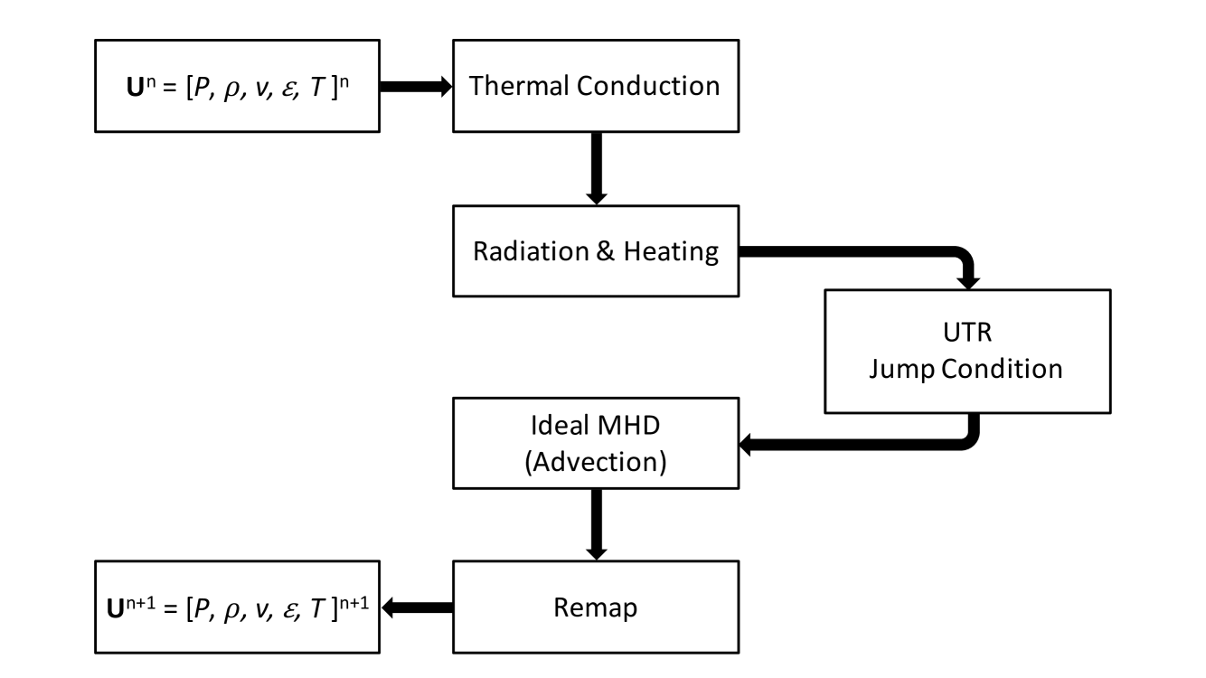
Figure 10: Lare1D with Thermal Conduction and Radiation time-splitting update strategy. The modification to include the UTR jump condition is also outlined. This step is ignored when the Lare1D code is employed without the jump condition.

A.3 Optically thin radiation (OTR)

For the optically thin radiative loss function we use a piecewise continuous power law,

$$\hskip 85.35826ptL_{r}=n^{2}\chi T^{\alpha},$$ (28)

where the temperature dependent constants $\chi$ and $\alpha$ are defined following Klimchuk et al. (2008). In the time-splitting update, the radiation step is of the form,

$$\hskip 85.35826pt\rho\frac{\partial\epsilon}{\partial t}=-n^{2}\chi T^{\alpha},$$ (29)

which is integrated using a time-centred finite difference method (FDM). To prevent the plasma from catastrophically cooling under the effects of OTR, we impose a radiative time step restriction, $\Delta t_{rad}$, on the integration, that prevents the temperature (specific internal energy density) from decreasing by more than $1\%$ during a single time step. This radiative restriction is not as severe as the advective time step (21) but can become important at the peak of the radiative losses.
To maintain our isothermal chromosphere, at a temperature of 10,000K, radiation is smoothly turned off over a $100$K interval, above the chromospheric temperature (Klimchuk et al. 1987, BC13).

A.4 Heating

The Lare code deals with the effects of viscous heating during the advection step. However, we also include a separate heating step of the form,

$$\hskip 85.35826pt\rho\frac{\partial\epsilon}{\partial t}=Q,$$ (30)

where our heating function, which is the dominant source of heating in our numerical simulations, is defined as the sum of contributions from both the background heating ($Q_{bg}$) and additional heating ($Q_{H}$),

$$\hskip 85.35826ptQ=Q_{bg}+Q_{H}.$$ (31)

The heating step is integrated using a simple FDM which we incorporate into the radiation step (29). This allows the temperature (specific internal energy density) to be updated due to the effects of optically thin radiation and heating simultaneously.

A.5 Time-splitting update

Let ${\bf U}=[P,\rho,v,\epsilon,T]$, be a vector of the model variables. The one-dimensional field-aligned MHD equations can then be written in terms of an ideal MHD component and non-ideal components,

$$\hskip 28.45274pt\dfrac{\partial{\bf U}}{\partial t}={\bf L}^{\textsc{c}}({\bf U})+{\bf L}^{\textsc{r}}({\bf U})+{\bf L}^{\textsc{mhd}}({\bf U}),$$ (32)

where ${\bf L}^{\textsc{c}}$, ${\bf L}^{\textsc{r}}$ and ${\bf L}^{\textsc{mhd}}$ are the thermal conduction, radiation and heating and ideal MHD operators respectively. During a single time step, we use the Lie-splitting (sequential splitting) method (Farago et al. 2011) to integrate these operators separately.
The temperature (specific internal energy density) is updated first, based on the effects of thermal conduction, OTR and heating, before the ideal field-aligned MHD equations are solved. Following this strategy, the Lie-splitting update for one complete time step is given by,

$$\hskip 56.9055pt\bf{U}^{*} = {\bf{C(U}}^{n},\Delta t),$$

$$\bf{U}^{**} = {\bf{R(U}}^{*},\Delta t),$$

$$\bf{U}^{n+1} = {\bf{MHD(U}}^{**},\Delta t),$$ (33)

where ${\bf{U}}^{n+1}={\bf{C}(U}^{n},\Delta t)$, ${\bf{U}}^{n+1}={\bf{R}(U}^{n},\Delta t)$ and ${\bf{U}}^{n+1}={\bf{MHD}(U}^{n},\Delta t)$ represent the updates of thermal conduction, radiation and heating and ideal MHD, for the time step $\Delta t$. This update strategy is shown in Fig. 10
Since we treat thermal conduction using STS methods we super-step the conductive timescale restriction (accelerate the explicit sub-cycling). Therefore, the time-splitting strategy (33) stably integrates the field-aligned MHD equations, on a time step that is given by,

$$\hskip 56.9055pt\Delta t=\textrm{min}\,(\Delta t_{adv},\,\Delta t_{rad}).$$ (34)

Appendix B Super time stepping methods to treat thermal conduction

Table 3: Numerical simulation computation times (run on a single processor) for three different methods to treat thermal conduction.

Case	$N_{z}$	$\tau_{\textrm{sts}}$	$\tau_{\textrm{cyc}}$	$\tau_{\textrm{exp}}$	$\tau_{\textrm{cyc}}$/	$\tau_{\textrm{exp}}$/
		(mins)	(mins)	(mins)	$\tau_{\textrm{sts}}$	$\tau_{\textrm{sts}}$
1	500	2.45	1.98	2.25	0.81	0.92
	1,000	6.73	6.47	15.72	0.96	2.34
	2,000	12.23	29.07	128	2.38	10.5
	4,000	42.6	199	592	4.67	13.9
	8,000	205	1,537	4,699	7.50	22.9
2	500	6.32	8.12	25.7	1.28	4.07
	1,000	18.5	45.02	122	2.43	6.59
	2,000	48.8	308	970	6.31	19.9
	4,000	135	2,385	7,772	17.7	57.6
	8,000	607	18,778	47,123*	30.9	77.6
3	500	12.15	33.13	168	2.73	13.8
	1,000	49.67	257	790	5.17	15.9
	2,000	138	2,023	6,238	14.7	45.2
	4,000	579	15,958	48,405*	27.6	83.6
	8,000	2,440	108,898*	238,620*	44.6	97.8

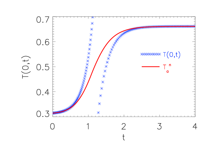
Figure 11: The panel shows the temporal evolution of $T(0,t)$. The solution leaves a thermally unstable isothermal equilibrium and approaches a new stable, non-isothermal equilibrium. The solid red curve is the numerical solution obtained by using the RKL2 STS method ($T^{n}_{a}$) and the blue asterisks represent the corresponding linear solutions ($T(0,t)$). The units on both axes are arbitrary.

In the interests of computational efficiency, to relax the conductive timescale stability restriction of an explicit method $(\Delta t_{cond}\leq\rho(\Delta z)^{2}/(2\kappa_{0}T^{5/2}))$, we treat thermal conduction by using super time stepping (STS) methods, as described in Meyer et al. (2012, 2014). These methods are essentially an acceleration of explicit time step sub-cycling and have been used effectively to speed up the integration of parabolic operators. In particularly, we use the Runge-Kutta Legendre method with second-order temporal accuracy (RKL2).
Extending on the test problems considered in Meyer et al. (2012, 2014), we have tested the RKL2 method for appropriateness of use in coronal plasma conditions, in order to ensure that the increased conductive time step does not influence the correct temporal evolution. The Zel’dovich problem of a propagating conduction front (Zel’dovich & Raizer 1967) has been solved.
In addition, we investigate whether or not STS methods can correctly obtain the growth (decay) rate when leaving (approaching) a thermally unstable (stable) isothermal (non-isothermal) equilibrium. Using a model equation, under the assumption of constant density, we solve the boundary value problem,

$$\dfrac{\partial T}{\partial t}=-\dfrac{\partial}{\partial z}\left(-T^{5/2}\dfrac{\partial T}{\partial z}\right)-\chi T^{\alpha}+H,\ -1/2\leq z\leq 1/2,$$

$$T(-1/2,t)=T(1/2,t)=T_{0},$$ (35)

with the initial condition,

$$T(z,0)=T_{0}+\bar{T_{1}}\cos(\pi z),\quad-1/2\leq z\leq 1/2.$$

$T_{0}$ is the isothermal unstable equilibrium and $\bar{T_{1}}\cos(\pi z)$ is a small perturbation. Linearising equation (35), the temperature grows as,

$$\hskip 56.9055ptT(0,t)=T_{0}+\bar{T_{1}}(0)e^{\sigma t},$$ (36)

with $\sigma=-\pi^{2}T_{0}^{5/2}-\alpha{\chi}T_{0}^{{\alpha}-1}$. Fig. 11 shows the temporal evolution of $T(0,t)$ using the STS method, as a solid red curve labelled $T_{a}^{n}$. The linear solution (36) is shown as asterisks and the exact growth rate matches the rate calculated from the computational solution. A similar analysis confirms that the exact decay rate, as the temperature evolves towards the non-isothermal stable equilibrium, is also correctly predicted by the STS method. Therefore, we believe that STS methods are appropriate for use in solving more complex coronal plasma based problems, where the effect of thermal conduction plays an important role.
Although STS methods have already been implemented in some 3D MHD codes (e.g. Reale et al. 2016, in press.) it remains instructive here to present a quantification of the computational gains involved. Based on the computation time ratios in Table 3, the benefit of using STS methods is immediately clear, especially as the coronal temperature, which scales strongly with the heating event, increases and the conductive timescale decreases.

References

- Antiochos & Sturrock (1978) Antiochos, S. K. & Sturrock, P. A. 1978, ApJ, 220, 1137
- Arber et al. (2001) Arber, T. D., Longbottom, A. W., Gerrard, C. L., & Milne, A. M. 2001, Journal of Computational Physics, 171, 151
- Betta et al. (1997) Betta, R., Peres, G., Reale, F., & Serio, S. 1997, A&AS, 122
- Bourdin et al. (2013) Bourdin, P.-A., Bingert, S., & Peter, H. 2013, A&A, 555, A123
- Bradshaw & Cargill (2006) Bradshaw, S. J. & Cargill, P. J. 2006, A&A, 458, 987
- Bradshaw & Cargill (2010a) Bradshaw, S. J. & Cargill, P. J. 2010a, ApJ, 710, L39
- Bradshaw & Cargill (2010b) Bradshaw, S. J. & Cargill, P. J. 2010b, ApJ, 717, 163
- Bradshaw & Cargill (2013) Bradshaw, S. J. & Cargill, P. J. 2013, ApJ, 770, 12
- Bradshaw & Mason (2003) Bradshaw, S. J. & Mason, H. E. 2003, A&A, 407, 1127
- Cargill et al. (2012a) Cargill, P. J., Bradshaw, S. J., & Klimchuk, J. A. 2012a, ApJ, 752, 161
- Cargill et al. (2012b) Cargill, P. J., Bradshaw, S. J., & Klimchuk, J. A. 2012b, ApJ, 758, 5
- Cargill et al. (2015) Cargill, P. J., Warren, H. P., & Bradshaw, S. J. 2015, Philosophical Transactions of the Royal Society of London Series A, 373, 20140260
- Dahlburg et al. (2016) Dahlburg, R. B., Einaudi, G., Taylor, B. D., et al. 2016, ApJ, 817, 47
- Farago et al. (2011) Farago, I., Havasi, A., & Horvath, R. 2011, International Journal of Numerical Analysis and Modeling, 2, 142
- Fletcher & De Pontieu (1999) Fletcher, L. & De Pontieu, B. 1999, ApJ, 520, L135
- Hansteen et al. (2015) Hansteen, V., Guerreiro, N., De Pontieu, B., & Carlsson, M. 2015, ApJ, 811, 106
- Hood et al. (2016) Hood, A. W., Cargill, P. J., Browning, P. K., & Tam, K. V. 2016, ApJ, 817, 5
- Klimchuk et al. (1987) Klimchuk, J. A., Antiochos, S. K., & Mariska, J. T. 1987, ApJ, 320, 409
- Klimchuk et al. (2008) Klimchuk, J. A., Patsourakos, S., & Cargill, P. J. 2008, ApJ, 682, 1351
- Meyer et al. (2012) Meyer, C. D., Balsara, D. S., & Aslam, T. D. 2012, MNRAS, 422, 2102
- Meyer et al. (2014) Meyer, C. D., Balsara, D. S., & Aslam, T. D. 2014, Journal of Computational Physics, 257, 594
- Reale (2014) Reale, F. 2014, Living Reviews in Solar Physics, 11
- Reale et al. (2016) Reale, F., Orlando, S., Guarrasi, M., et al. 2016, ApJ in press
- Spitzer (1962) Spitzer, L. 1962, Physics of Fully Ionised Gases
- Vesecky et al. (1979) Vesecky, J. F., Antiochos, S. K., & Underwood, J. H. 1979, ApJ, 233, 987
- Zacharias et al. (2011) Zacharias, P., Peter, H., & Bingert, S. 2011, A&A, 531, A97
- Zel’dovich & Raizer (1967) Zel’dovich, Y. B. & Raizer, Y. P. 1967, Physics of shock waves and high-temperature hydrodynamic phenomena