LTH 1098, TTP16-034

Four loop renormalization of the Gross-Neveu model

J.A. Gracey

Theoretical Physics Division, Department of Mathematical Sciences, University of Liverpool, P.O. Box 147, Liverpool, L69 3BX, United Kingdom

T. Luthe

Institut für Theoretische Teilchenphysik, Karlsruhe Institute of Technology (KIT), Karlsruhe, Germany

Y. Schröder

Grupo de Fisica de Altas Energias, Universidad del Bio-Bio, Casilla 447, Chillan, Chile

Abstract. We renormalize the $SU(N)$ Gross-Neveu model in the modified minimal subtraction ($\overline{\mbox{MS}}$) scheme at four loops and determine the $\beta$-function at this order. The theory ceases to be multiplicatively renormalizable when dimensionally regularized due to the generation of evanescent $4$-fermi operators. The first of these appears at three loops and we correctly take their effect into account in deriving the renormalization group functions. We use the results to provide estimates of critical exponents relevant to phase transitions in graphene.

1 Introduction

The Gross-Neveu model with an $O(N)$ or $SU(N)$ symmetry is a quantum field theory of spin-$\frac{1}{2}$ fields which interact quartically, [1]. It is also known as the Ashkin-Teller model, [2]. Aside from being perturbatively renormalizable in two dimensions rather than four it has many properties which are in common with Quantum Chromodynamics (QCD). For instance, it is asymptotically free and has dynamical symmetry breaking whereby the classically massless fermions become massive in the true vacuum, [1]. These together with other properties such as the existence of an exact $S$-matrix, [3], which provides the full bound state spectrum of the quantum theory, mean that the Gross-Neveu model has been used for many years as a laboratory to examine ideas which are harder to gain insight into in higher dimensional theories such as QCD.

The theory is also of interest due to its connections with problems in condensed matter theory. For example, it has been shown that in the so-called replica limit, $N$ $\to$ $0$, the $SU(N)$ theory describes the physics of the random bond Ising model, [4]. See [5], for instance, for a review article. More recently, the Gross-Neveu model has been found to be connected to problems in conformal field theory (CFT) in dimensions greater than two. Specifically it lies in the same universality class at the Wilson-Fisher fixed point in $d$-dimensions as the Gross-Neveu-Yukawa theory whose critical dimension is four.

Aside from the Ising model connection, [4], which has been explored recently in the CFT context using the conformal bootstrap programme, [6], the Gross-Neveu model has connections with recent developments in AdS/CFT theories. For example, see [7] for a recent review on the background to this area. Given this particular relation to current problems in higher dimensional quantum field theories, it is worth noting that that analysis rests on performing computations with the large $N$ or $1/N$ expansion. This expansion parameter, which is an alternative to conventional perturbation theory, is another feature which the Gross-Neveu model shares with QCD. In the latter case one can perform large $N_{\!c}$ or large $N_{\!f}$ expansions where $N_{\!c}$ and $N_{\!f}$ are the number of colours or (massless) quark flavours respectively. One advantage of an analysis using the large $N$ expansion in the Gross-Neveu model, or large $N_{\!f}$ in the case of QCD, is that each theory is renormalizable away from the critical dimension of either quantum field theory.

Given the centrality of the Gross-Neveu model to a wide range of applications since its introduction, [1], it is worth noting that it has not been renormalized in perturbation theory to as high a loop order as several of the other basic theories such as $O(N)$ scalar $\phi^{4}$ theory or QCD itself. For instance, after the one loop results of [1] the two loop renormalization was carried out in [8] and verified in [9]. Subsequently, the three loop renormalization was performed in [10] with the $\beta$-function appearing independently in [11, 12]. At four loops the wave function and mass anomalous dimensions were determined in [13]. However, from the point of view of determining critical exponents in the replica limit, say, the information in these four loop terms is of no use until the $\beta$-function is known to that order too as it contains the location of the critical point to the same precision. This is the purpose of the article where we will complete the full four loop renormalization of the $SU(N)$ Gross-Neveu model by determining the coupling constant renormalization constant in the modified minimal subtraction ($\overline{\mbox{MS}}$) scheme. In terms of time lines this is a quarter of a century since the three loop $\beta$-function of [11, 12]. While relatively long this is not dissimilar to the other basic theories mentioned already. For instance, the step from five, [14, 15], to six loops, [16, 17, 18], for the scalar $\phi^{4}$ theory in four dimensions also took twenty-five years. Similarly from the appearance of the four loop $\overline{\mbox{MS}}$ QCD $\beta$-function, [19], and its verification [20], until the recent $\overline{\mbox{MS}}$ evaluation for $SU(3)$, [21], the time interval was nearly a score of years. The seven loop wave function renormalization of $\phi^{4}$ theory has also been determined recently with an indication that the $\beta$-function could be available soon outside the normal waiting period, [17].

What is central to all these recent increases in the loop order of the $\beta$-functions has been the advance in computational technology. This does not solely mean computer hardware and speed. More crucial has been the creation, for instance, of an overall algorithm to handle the inordinate amount of integration by parts of the exponentially large number of Feynman diagrams which occur at successive loop orders, [22]. A consequence of this algorithm is the need to determine explicitly the value of a relatively small subset of integrals, termed masters, which cannot be computed using integration by parts. One such approach has been to evaluate these numerically to very high precision using difference relations, [23]. Then analytic values can be adduced using the integer finding method of [24] and a basis of transcendentals, such as multiple zeta values (MZV). Alternatively these difficult master integrals can in certain situations be determined directly by algebraic methods. For instance, high level mathematics, such as algebraic geometry and the development of the theory and properties of hyperlogarithms and MZVs, have crystallized into an algorithm such that all the parameter integrations in the Schwinger representation of certain master Feynman integrals can be found. For instance, this approach has been encoded in the Hyperint package, [25].

Given this background we have applied the latest machinery to tackle the four loop $\overline{\mbox{MS}}$ evaluation of the Gross-Neveu $\beta$-function. It transpires that this is not as straightforward as for the parallel computation in scalar field theories and to a lesser extent than for QCD. This is because in dimensionally regularizing the Gross-Neveu model, as is the usual regularization for multiloop renormalization of such theories, one loses multiplicative renormalizability, [26, 27, 28], which was observed in detail in [29, 30]. In essence, as with the treatment of $4$-fermi operators in effective field theories in four dimensions, evanescent operators are generated. These are operators which exist in $d$-dimensions but are absent in the critical dimension of the actual field theory being renormalized. Their presence in the regularized theory cannot be ignored, as has been noted in the Gross-Neveu context, [29, 30, 13], since they have an effect on the determination of the renormalization group functions in the lifting of the regularization. However, in the Gross-Neveu model the effect of these evanescent operators on the renormalization group functions does not become manifest until four loops. This was recognized in [28, 29, 30] and implemented in the construction of the four loop mass anomalous dimension in [13]. Useful in this respect was the formalism developed to account for the effect the evanescence has on the renormalization group functions given in [26, 27]. Like scalar $\phi^{4}$ theory the wave function anomalous dimension has no one loop term. So the effect of the evanescent operators will not be apparent before five loops for that particular renormalization group function. Given our interest in the four loop $\beta$-function here we will be careful in computing the underlying $4$-point function which determines the coupling constant renormalization and in the same instance find the new evanescent operators which are generated at four loops. These will be required for any future five loop renormalization.

The article is organized as follows. Section $2$ is devoted to reviewing the formalism required to renormalize two dimensional theories with a $4$-fermi interaction via the projection method of [26, 27]. The technical details of how we evaluated the four loop Feynman graphs contributing to the renormalization of the $4$-point function are given in section $3$. The main result for the $\beta$-function is given in section $4$ and applications to problems in condensed matter theory are given in section $5$. We provide brief concluding remarks in section $6$. There are two appendices which respectively detail the tensor reduction construction and the numerical and analytic form of the master integrals up to and including four loops.

2 Preliminaries

We begin by summarizing the essential ingredients required to renormalize the $SU(N)$ Gross-Neveu model to four loops in the $\overline{\mbox{MS}}$ scheme. The technical details as to how the computations are performed will be devolved to a later section. We have chosen to consider the $SU(N)$ theory rather than the $O(N)$ model because the former formulation has fewer terms in the vertex Feynman rule. Hence it minimizes the number of algebraic manipulations in the computations. The $O(N)$ renormalization group functions can be reconstructed from the final $SU(N)$ results.

The bare $SU(N)$ Gross-Neveu Lagrangian is, [1],

$$L~{}=~{}i\bar{\psi}_{0}^{i}\partial\!\!\!/\psi^{i}_{0}~{}-~{}m_{0}\bar{\psi}^{i}_{0}\psi^{i}_{0}~{}+~{}\frac{1}{2}g_{0}(\bar{\psi}^{i}_{0}\psi^{i}_{0})^{2}$$ (2.1)

where we use ₀ to denote a bare field or parameter and $g$ is the coupling constant. In general terms (2.1) is renormalizable in two dimensions, [1]. We have included a mass for the fermion here partly to be complete but also because we wish to avoid potential infrared issues when we come to computing the relevant Feynman diagrams. When one takes traces over $\gamma$-matrices the Feynman integrals will have propagators similar to those of a bosonic field. It is well known that in two dimensions a bosonic propagator is infrared divergent. So including a mass for the fermion will ensure that all emerging divergences are ultraviolet in nature. The technical problem which arises is that when one considers the theory in higher dimensions it ceases to be renormalizable since the interaction produces a dimensionful coupling constant. This observation has implications when one dimensionally regularizes (2.1) to initiate its renormalization. Specifically (2.1) ceases to be multiplicatively renormalizable, [26, 27]. Instead evanescent operators are generated in $d$-dimensions whose presence affects the derivation of the true renormalization group functions. This has been recognized in the earlier work of [26, 27, 28, 29, 30]. Moreover, a procedure has been developed to account for the effect of these evanescent operators, [26, 27], which we will use and extend to the case of the $\beta$-function computation here. To appreciate the issue in more depth it is instructive to recall the properties of the $\gamma$-algebra. In strictly integer dimensions the $\gamma$-matrices satisfy the Clifford algebra

$$\{\gamma^{\mu},\gamma^{\nu}\}~{}=~{}2\eta^{\mu\nu}~{}.$$ (2.2)

However when the spacetime dimension $d$ becomes a continuous variable the matrices $\gamma^{\mu}$ cease to span the spinor space. Instead the basis of $\gamma$-matrices needs to be expanded to a new set of matrices denoted by $\Gamma^{\mu_{1}\ldots\mu_{n}}_{(n)}$ for all integers $n$ $\geq$ $0$. We have chosen to use the basis and definition of [26, 30, 31, 32, 33] and they are defined by

$$\Gamma_{(n)}^{\mu_{1}\mu_{2}\ldots\mu_{n}}~{}=~{}\gamma^{[\mu_{1}}\gamma^{\mu_{2}}\ldots\gamma^{\mu_{n}]}$$ (2.3)

where a factor of $1/n!$ is understood within the total antisymmetrization on the right hand side. To clarify when $d$ is an integer dimension $D$, say, then the basis of $\Gamma$-matrices is finite. This is because $\Gamma_{(n)}^{\mu_{1}\mu_{2}\ldots\mu_{n}}$ $=$ $0$ for $n$ $>$ $D$ due to the antisymmetrization. Although we are considering the non-chiral Gross-Neveu model, (2.1), it is worth noting that $\Gamma_{(5)}^{\mu_{1}\mu_{2}\mu_{3}\mu_{4}\mu_{5}}$ has no relation to the usual $\gamma^{5}$ matrix. The renormalization of the chiral Gross-Neveu model is more involved, [26, 27], and beyond our present considerations.

With these generalized $\gamma$-matrices the dimensionally regularized Gross-Neveu model can be regarded as a special case of the more general $d$-dimensional Lagrangian, [26, 27],

$$L~{}=~{}i\bar{\psi}_{0}^{i}\partial\!\!\!/\psi^{i}_{0}~{}-~{}m_{0}\bar{\psi}^{i}_{0}\psi^{i}_{0}~{}+~{}\frac{1}{2}\sum_{n=0}^{\infty}g_{(n)\,0}\,\bar{\psi}^{i}_{0}\Gamma_{(n)}^{\mu_{1}\ldots\mu_{n}}\psi^{i}_{0}\,\bar{\psi}^{i}_{0}\Gamma_{(n)~{}\mu_{1}\ldots\mu_{n}}\psi^{i}_{0}$$ (2.4)

where $g_{(n)}$ are generalized couplings. Although we will always use $g$ $=$ $g_{(0)}$ which is not to be confused with the bare coupling constant. The additional couplings $g_{(n)}$ fall into two classes. For (2.1) $g_{(1)}$ and $g_{(2)}$ would correspond to renormalizable interactions in strictly two dimensions and are not couplings associated with evanescent interactions. The former coupling corresponds to the Thirring model while the latter is related to the interaction $\frac{1}{2}(\bar{\psi}^{i}\gamma^{5}\psi^{i})^{2}$ which is part of the chiral Gross-Neveu model. We do not consider either of these theories here. Although the projection formalism of [26, 27] applies equally to their renormalization. The couplings $g_{(n)}$ with $n$ $\geq$ $3$ label the set of evanescent operators, defined by

$${\cal O}_{n}~{}=~{}\mbox{\small{$\frac{1}{2}$}}\bar{\psi}^{i}\Gamma_{(n)}^{\mu_{1}\ldots\mu_{n}}\psi^{i}\,\bar{\psi}^{i}\Gamma_{(n)~{}\mu_{1}\ldots\mu_{n}}\psi^{i}~{},$$ (2.5)

which are necessary to ensure (2.1) is renormalizable. These operators will be generated in the renormalization of (2.1) itself. For (2.4) such operators are generated but in the sense that this is hidden as their divergences are removed by the renormalization constants associated with $g_{(n)}$. For (2.1), [29, 30], the first new operator, ${\cal O}_{3}$, emerges first at three loops. In other words there was a term in the $4$-point function of (2.1) at three loops of the form

$$\frac{a_{(3)}}{\epsilon}\Gamma^{\mu\nu\sigma}_{(3)}\otimes\Gamma_{(3)\,\mu\nu\sigma}$$ (2.6)

where $a_{(3)}$ is the residue of the simple pole in the regularizing parameter $\epsilon$ with $d$ $=$ $2$ $-$ $2\epsilon$. The tensor product notation is understood to mean the different spinor channels into which the operator $O_{(n)}$ can be decomposed in the $4$-point function. While the operator ${\cal O}_{(3)}$ is non-existent in strictly two dimensions its generation in dimensional regularization cannot be overlooked as its presence will affect the extraction of the true renormalization group functions.

There are several ways of considering (2.4) from the practical point of renormalizing the $SU(N)$ Gross-Neveu model, (2.1). One could take a general approach beginning with the most general extension of (2.1) which is (2.4) with $g_{(1)}$ $=$ $g_{(2)}$ $=$ $0$ at the outset and then compute all the renormalization constants for the field, mass and the coupling constants $g_{(n)}$ with $n$ $\neq$ $1$ and $2$, to four loops. From the resultant renormalization group functions then the $\beta$-function for $g$ can be extracted. An alternative approach would be to ignore the full set of couplings and instead include the $g$-dependent renormalization constants for the various evanescent operators as and when they are generated. The true $\beta$-function for $g$ can then be determined using the projection formalism. The generated operators, such as (2.6), have a hidden effect on the renormalization at the first loop order beyond that of when they appear. This has to be accounted for in extracting the renormalization group functions which one would find if the regularization of the two dimensional Lagrangian was not in fact dimensional.

To summarize [26, 27] there are three essential aspects to the construction of the renormalization group functions. The first is the determination of what are called the naive renormalization group functions which are denoted by $\tilde{\gamma}(g)$, $\tilde{\gamma}_{m}(g)$ and $\tilde{\beta}(g)$ for the wave function, mass and coupling constant renormalizations respectively, [26, 27]. They are constructed in the standard way of renormalizing a quantum field theory with the proviso that when an evanescent operator is generated, it is included in the Feynman rules for the renormalization at all subsequent higher orders. Associated with the evanescent operator generation is its own $\beta$-function, denoted by $\beta_{k}(g)$, which is the second aspect of the construction where we will use the label $k$ to refer to the strictly evanescent quantities and thus $k$ $\geq$ $3$ in two dimensions. For the case of (2.6) the residue $a_{(3)}$ is in effect the first term of $\beta_{3}(g)$ which was computed in [29, 30, 13]. We concentrate here on the formalism and give explicit details later. However, in the context of the interpretation of (2.4) in terms of generated operators without the generalized couplings $g_{(k)}$ then to three loops the dimensionally regularized Lagrangian which is used to determine the renormalization group functions of the strictly two dimensional theory is, [28, 29, 30, 13],

$$L~{}=~{}iZ_{\psi}\bar{\psi}^{i}\partial\!\!\!/\psi^{i}~{}-~{}mZ_{\psi}Z_{m}\bar{\psi}^{i}\psi^{i}~{}+~{}\frac{1}{2}g\mu^{2\epsilon}Z_{g}Z^{2}_{\psi}(\bar{\psi}^{i}\psi^{i})^{2}~{}+~{}\frac{1}{2}g\mu^{2\epsilon}Z_{33}Z^{2}_{\psi}\left(\bar{\psi}^{i}\Gamma_{(3)}^{\mu\nu\sigma}\psi^{i}\right)^{2}~{}.$$ (2.7)

Here $Z_{33}$ is the counterterm for (2.6) and $\mu$ is the scale introduced to ensure that the coupling constants are dimensionless in $d$-dimensions. In (2.7) we have used the standard definitions of the renormalization constants which connect bare with renormalized quantities which are

$$\psi_{0}~{}=~{}\psi\sqrt{Z_{\psi}}~{}~{}~{},~{}~{}~{}m_{0}~{}=~{}mZ_{m}~{}~{}~{},~{}~{}~{}g_{0}~{}=~{}gZ_{g}\mu^{2\epsilon}~{}.$$ (2.8)

In the context of (2.4) $Z_{33}$ would correspond to the renormalization of the coupling $g_{(3)}$ as would $Z_{nn}$ be the obvious generalization for the other couplings $g_{(n)}$. Moreover, all these renormalization constants would be functions of the complete set of couplings. However, when one considers the reduced non-multiplicatively renormalizable Lagrangian (2.1) then only the necessary evanescent operator coupling constants are included and they will depend only on $g$. This means that the first term of $Z_{33}$, for instance, does not begin with unity like $Z_{g}$.

The final part of the projection formalism is the computation of the underlying projection functions for the wave function, mass and coupling constant and denoted by $\rho^{(k)}(g)$, $\rho^{(k)}_{m}(g)$ and $C^{(k)}(g)$ respectively. They are defined and computed through the projection formula, [26, 27],

$$\left.\int d^{d}x\,{\cal N}[{\cal O}_{k}]\right|_{g_{(i)}=0\,,\,d=2} = \int d^{d}x\left(\,\rho^{(k)}(g){\cal N}[i\bar{\psi}\partial\!\!\!/\psi~{}-~{}m\bar{\psi}\psi~{}+~{}2g{\cal O}_{0}]\right.$$ (2.9)

$$\left.\left.~{}~{}~{}~{}~{}~{}~{}~{}~{}-~{}\rho^{(k)}_{m}(g)\,{\cal N}[m\bar{\psi}\psi]~{}+~{}C^{(k)}(g){\cal N}[{\cal O}_{0}]\right)\right|_{g_{(i)}=0\,,\,d=2}$$

where ${\cal N}[{\cal O}_{k}]$ denotes the normal ordering of the evanescent operator ${\cal O}_{k}$, $k$ $\geq$ $3$. While we will follow the method of [26, 27] we note that a similar projection method for evanescent $4$-fermi operators was provided in [34]. In practical terms the relation (2.9) is to be regarded as having meaning only inside a Green’s function. For our purposes these will be $2$- and $4$-point functions. One evaluates the insertion of ${\cal N}[{\cal O}_{k}]$ in either $n$-point function to a certain order in perturbation theory. Then the operators on the right hand side are inserted in the same $n$-point function to the same order. After the usual operator renormalization the evanescent couplings are set to zero and the Green’s function determined in strictly two dimensions which is the meaning of the restriction ${g_{(i)}=0\,,\,d=2}$, [26, 27]. The final task is to deduce the perturbative expansions of the three projection functions with $\rho^{(k)}(g)$ and $\rho^{(k)}_{m}(g)$ being determined from insertion in a $2$-point function and $C^{(k)}(g)$ from the $4$-point function. Finally, once the naive renormalization group functions, evanescent operator $\beta$-functions and projection functions are known to the loop order necessary for the order the true two dimensional renormalization group functions are needed then these are given by evaluating, [26, 27],

$$\beta(g) = \tilde{\beta}(g)~{}+~{}\sum_{k=3}^{\infty}C^{(k)}(g)\beta_{k}(g)$$

$$\gamma(g) = \tilde{\gamma}(g)~{}+~{}\sum_{k=3}^{\infty}\rho^{(k)}(g)\beta_{k}(g)$$

$$\gamma_{m}(g) = \tilde{\gamma}_{m}(g)~{}+~{}\sum_{k=3}^{\infty}\rho^{(k)}_{m}(g)\beta_{k}(g)~{}.$$ (2.10)

In (2.10) the naive renormalization group functions are derived in the standard fashion through

$$\tilde{\gamma}(g) = \mu\frac{\partial}{\partial\mu}\ln Z_{\psi}~{}~{}~{},~{}~{}~{}\tilde{\gamma}_{m}(g)~{}=~{}-~{}\tilde{\beta}(g)\frac{\partial}{\partial g}\ln Z_{m}$$

$$\tilde{\beta}(g) = (d-2)g~{}-~{}g\tilde{\beta}(g)\frac{\partial}{\partial g}\ln Z_{g}$$ (2.11)

once all the renormalization constants have been computed. In [28, 29, 30, 13] the three projection functions were evaluated explicitly to the requisite loop order to be able to deduce the renormalization group functions to four loops. Although in the case of the wave function renormalization for (2.1) the leading term of $\rho^{(3)}(g)$ is not required since there is no one loop correction to $\gamma(g)$. In the determination of $\gamma_{m}(g)$ at four loops an error was discovered in the original evaluation of $\beta_{3}(g)$, [28], and in a later article [35]. Both these articles were three loop analyses and $\beta_{3}(g)$ had not been used or tested in the application of the projection formalism to a four loop computation. While both these articles agreed on the rational part of $\beta_{3}(g)$ they differed in the irrational term. This was resolved in [13] when $\gamma_{m}(g)$ was computed to four loops. To achieve this it was first required to extract the correct value for the irrational part of $\beta_{3}(g)$. With the incorrect value of $\beta_{3}(g)$ the mass anomalous dimension does not vanish when $N$ $=$ $\frac{1}{2}$ as it ought to since there is no interaction for this value of $N$. The appearance of this rational value for $N$ can be understood best if one converts the $SU(N)$ theory, (2.1), to the case with Majorana fields whence there is an $O(2N)$ symmetry. Thus when $N$ $=$ $\frac{1}{2}$ here the $4$-fermi interaction vanishes due to the Grassmann property. Likewise we expect the true $\beta$-function of (2.1) to be zero when $N$ $=$ $1$. This is because in that case one can use a two dimensional Fierz identity to show that

$$(\bar{\psi}\psi)^{2}~{}=~{}-~{}\frac{1}{2}(\bar{\psi}\gamma^{\mu}\psi)^{2}~{}.$$ (2.12)

This means that the $N$ $=$ $1$ Lagrangian is equivalent to the abelian Thirring model whose $\beta$-function is known to be zero, [26, 27]. The presence of a factor of $(N-1)$ in each term of the three loop $\overline{\mbox{MS}}$ $\beta$-function of (2.1) is already established. However, to this order there is no contribution from $\beta_{3}(g)$ to the true $\beta$-function which will first occur at four loops. The emergence of another factor of $(N-1)$ at four loops will be an important check on our computations and the use of the projection formalism.

3 Computational technicalities

We devote this section to the technical issues surrounding the evaluation of the Feynman diagrams and the organization of the renormalization. In lower loop renormalization of (2.1) several renormalization group functions were determined in the massless Lagrangian. For instance, the wave function anomalous dimension was derived at three loops in this way, [10]. That was possible since no infrared problems were introduced in the $2$-point function in the massless case and there are no exceptional momentum configurations in this Green’s function. By contrast the computation of the three loop $\beta$-function was carried out in several different ways. In [12] the interaction of (2.1) was first rewritten in terms of an auxiliary field, $\sigma$, before the massive Lagrangian with two couplings was renormalized and the three loop effective potential for $\sigma$ was computed. Independently in [11] the Lagrangian (2.1) was renormalized without introducing an auxiliary field. Later the three loop renormalization was revisited in [28, 29, 30] where the generation of the evanescent operator ${\cal O}_{3}$ was noted.

While this summarizes the previous higher order loop computations in the Gross-Neveu model to proceed to four loops we have followed a more systematic algorithm. We will renormalize the $2$- and $4$-point functions of (2.1) using the vacuum bubble approach of [36, 37] which was developed in order to simplify the renormalization of four dimensional theories. In this method one expands the massive propagators of (2.1) using the identity

$$\frac{1}{[(k-p)^{2}+m^{2}]}~{}=~{}\frac{1}{[k^{2}+m^{2}]}~{}+~{}\frac{[2kp-p^{2}]}{[k^{2}+m^{2}][(k-p)^{2}+m^{2}]}~{}.$$ (3.1)

The repeated use of this identity systematically replaces propagators involving an external momentum, $p$, with propagators involving purely internal loop momenta $k$. One terminates the expansion using Weinberg’s theorem, [38]. The algorithm was introduced in [37] for massless gauge theories. However, applying it to (2.1) with the particle mass already present means that an intermediate infrared regularizing mass does not need to be introduced in this application unlike [37]. In using this method for (2.1) it is virtually a trivial application. It is only in the case of the $2$-point function when it is multiplied by $p\!\!\!/$ and the spinor trace taken that one has to iterate the identity more than once to the termination point. For the extraction of the mass renormalization taking a spinor trace of the $2$-point function the first application of (3.1) in effect sets the external momentum to zero. A similar situation applies in part for the $4$-point function where in effect all external momenta are nullified at the outset. As part of the vacuum bubble algorithm described in [36, 37] the next stage is the evaluation of the resultant vacuum bubble graphs which emerge. The standard approach nowadays is to use the Laporta algorithm, [22]. This is a method which first constructs relations between Feynman integrals using identities established by integration by parts. These algebraic relations can then be solved by linear algebra in such a way that all integrals can be expressed in terms of a relatively small set of what are called master integrals. The $\epsilon$ expansion of these integrals are determined by non-integration by parts methods which completes the evaluation of all constituent integrals lurking within a Feynman graph of a Green’s function.

We have described the background to the approach of [36, 37] as a reference for the Gross-Neveu model renormalization here partly as we will make use of it but mainly because we have had to adapt it given the complication with the generation of ${\cal O}_{n}$. First, what is evident from (3.1) is that the Feynman integrals have scalar products of the internal and external momenta in the numerators. As the first part of the Laporta technique these are replaced by combinations involving the propagators themselves. If there is an irreducible scalar product the integral is what is termed completed by the inclusion of a propagator not associated with the original topology. This additional propagator contains the irreducible scalar product. One feature of the Laporta algorithm’s power is that it can handle such irreducible propagators. While this is the standard procedure there is a complication when we consider the $4$-point function of (2.1). If one did not have to account for the evanescent operator generation one would take a spinor projection of the Green’s function to access one channel of the Feynman rule and evaluate the resultant Feynman graphs. Instead we have to be more systematic and not take any spinor traces for the $4$-point function. This means that before we can evaluate any $4$-point function graph we first disentangle the internal momenta from contractions within $\gamma$-matrix strings. This leaves Feynman integrals which involve Lorentz tensors of the internal momenta up to rank $2L$ at $L$ loops. These internal momenta arise from the fermionic propagator. However, only an even number of internal momenta arise since we have already applied the vacuum bubble expansion and a vacuum bubble integral with an odd number of Lorentz indices is automatically zero. What remains to be done is to rewrite these Lorentz tensor integrals in terms of scalar products whence the earlier algorithm can be applied. It transpires that there is a large number of different combinations of internal momenta in the tensor integrals. Rather than develop a result for all possible cases we were able to construct a general tensor decomposition up to rank 8 for all combinations of internal momenta. This is more appropriate given how large a number occur at four loops. More details on the tensor decomposition is provided in appendix A.

As all the graphs can now be expanded in terms of completely massive scalar vacuum bubbles the next task is to reduce these to the set of masters. We have used the Reduze package, [39, 40], which is a C++ coding of the Laporta algorithm. It systematically constructs a database of the relations between all the required integrals and the final masters. One advantage of our approach is that we have needed only one integral family at each loop order to cover all possible integrals which arise. To three loops this is effectively trivial since the number of propagators in each integral family exactly matches the number of independent scalar products of the internal momenta. At four loops there are $10$ possible scalar products but since we have a single quartic interaction then at most there are eight propagators in a Feynman graph. So for the four loop integral family we have chosen the ordered propagators

$$\left\{\frac{1}{[k_{1}^{2}+m^{2}]},\frac{1}{[k_{2}^{2}+m^{2}]},\frac{1}{[k_{3}^{2}+m^{2}]},\frac{1}{[k_{4}^{2}+m^{2}]},\frac{1}{[(k_{1}-k_{4})^{2}+m^{2}]},\frac{1}{[(k_{2}-k_{4})^{2}+m^{2}]},~{}~{}~{}~{}~{}~{}~{}~{}~{}~{}\right.$$

$$\left.\frac{1}{[(k_{3}-k_{4})^{2}+m^{2}]},\frac{1}{[(k_{1}-k_{2})^{2}+m^{2}]},\frac{1}{[(k_{1}-k_{3})^{2}+m^{2}]},\frac{1}{[(k_{1}-k_{2}-k_{3})^{2}+m^{2}]}\right\}$$ (3.2)

as the integral family. One of the propagator choices to complete the family has been chosen to ensure a non-planar topology is covered. The application of Reduze produces a relatively small set of master integrals to be evaluated and substituted for the evaluation. These are illustrated in Figures $1$ and $2$. In Figure $2$ each dot on a line represents an increase in the power of the original propagator by unity. Although we have only illustrated the pure masters in the sense that beyond one loop one can have have products of lower loop order masters. For instance, one can have a product of $L$ one loop vacuum bubble graphs at each loop order $L$ or at four loops the product of the two loop master shown in Figure $1$ emerges as a master in Reduze at four loops. We note that the master integral labelled $1011.1.2$ in Figure $2$ is the only one which differs from the master basis choice in [41].

The final step is the determination of the $\epsilon$ expansion of the integrals in Figures $1$ and $2$. Aside from the simple one loop massive vacuum integral which is trivial to evaluate, at low loop order the leading term of the expansion of various integrals has already been found as well as a few simple ones at four loops, [13]. However, the known values are not sufficient to determine the divergence of the $4$-point function to the simple pole in $\epsilon$. This is partly because a subset of the full four loop masters were needed for the mass anomalous dimension computation and partly due to spurious poles which emerge when the integration by parts reduction is effected. In other words one has sometimes to evaluate a master to several finite orders in the $\epsilon$ expansion to ensure that the correct simple pole is found for the renormalization constant. Although it transpires that the higher orders in $\epsilon$ are ordinarily only required for those masters with a small number of propagators.

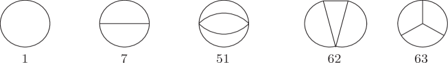
Figure 1: One, two and three loop master vacuum bubble integrals.

To find the values of the required terms in the $\epsilon$ expansion of the masters we have used the numerical method described in [22, 23]. Basically master integrals are evaluated numerically to very high precision by solving difference equations. The algorithm is not sensitive to the dimension of spacetime but needs to be applied separately for each integer. Originally, four loop massive vacuum bubbles were numerically determined in four space-time dimensions in [42]. Subsequently in [41] the analogous three dimensional set of masters was also determined to four loops to very high precision for applications to QCD at finite temperature. In repeating this exercise here at four loops for two dimensions, using algorithms developed in [44] as well as [45], we are providing the equivalent machinery which can be applied to parallel renormalization calculations in two dimensions.

However, the ultimate goal is to have renormalization group functions in terms of rationals as well as the Riemann $\zeta$-function. To four loops we do not expect any numbers other than those in keeping with our knowledge of the renormalization group functions in other theories to the same order in the $\overline{\mbox{MS}}$ scheme. This is a key observation mainly because in some of the low loop masters numbers other than (Riemann) zeta values appear in the the $\epsilon$ expansion. For instance, for the two loop master in Figure $1$ it is known that special values of the Clausen function such as $\mbox{Cl}_{2}(\mbox{\small{$\frac{\pi}{3}$}})$ contribute (see, for instance, [43, 13]). In [10, 13] the cancellation of this value in the evaluation of the renormalization constants was checked to three loops. A similar feature should emerge here. However, one first has to identify the presence of this and other such irrationals lurking within the numerical evaluation. This is possible through the application of the PSLQ algorithm of [24]. Fed with a basis of transcendentals that are expected to be contained in the numerical value, the algorithm tries to determine the actual linear combination of those basis numbers with rational coefficients. The robustness of the resulting explicit relation is tested against a more precise numerical evaluation of the coefficient in the $\epsilon$ expansion. With this approach we were able to determine all the necessary terms in the $\epsilon$ expansion of the masters of Figures $1$ and $2$ in order to be able to renormalize the $4$-point function of (2.1) to four loops, see appendix B.

The re-evaluation of the wave function and mass renormalization constants with the masters here was a check on the earlier computations of [10, 11, 12, 13] as well as being a partial check on certain values of the four loop masters we determined here. It transpired that for the simple pole associated with the generation of the new operator ${\cal O}_{4}$ at four loops a certain combination of higher order coefficients in the $\epsilon$ expansion of the masters was required. While each individual coefficient inevitably will contain rationals and irrationals aside from $\zeta_{n}$ we used PSLQ on the specific combination which emerged and searched successfully for a linear combination using the basis of $\{1,\zeta_{3},\zeta_{4},\zeta_{5}\}$. This is consistent with our expectations of the basis of numbers which appears in an $\overline{\mbox{MS}}$ renormalization group function at five loops, and the emerging linear relation can indeed be used to fix one expansion parameter, see (B.42). The effect the four loop generation of ${\cal O}_{4}$ has will become manifest at the next loop order similar to the effect ${\cal O}_{3}$ has in the four loop mass anomalous dimension in [13] and the $\beta$-function here. In appendix B we have recorded the $\epsilon$ expansion of the masters of Figures $1$ and $2$ to the various orders needed for our computations, both numerically and analytically, as well as more details of how the master values were found.

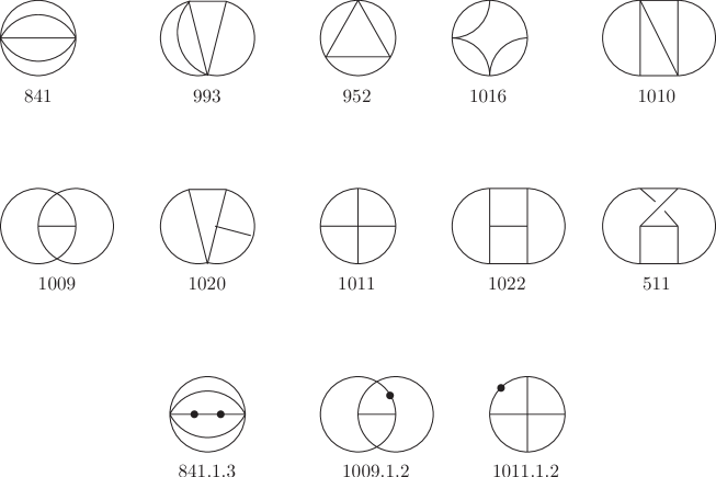
Figure 2: Four loop master vacuum bubble integrals. We label them by their sector identifier number, whose binary representation corresponds to the propagators (out of the set listed in (3)) that are present.

Running parallel to the treatment of the masters is the organization of the $\gamma$-matrices which had been stripped off to leave tensor integrals. In order to extract the naive coupling constant renormalization the $\gamma$-matrix strings have to be written in terms of the generalized matrices $\Gamma_{(n)}^{\mu_{1}\ldots\mu_{n}}$. To do this we exploit the algebraic properties of these matrices which was discussed at length in [28, 29, 30]. Products of $n$ $\gamma$-matrices can be decomposed into linear combinations of $\Gamma_{(r)}^{\mu_{1}\ldots\mu_{r}}$ where $r$ is even or odd depending on whether $n$ is even or odd. The range of $r$ begins with $0$ or $1$, depending on whether $n$ is even or odd respectively, and ends at $n$. One can construct the decomposition iteratively through the basic identities, [28, 29, 30],

$$\Gamma^{\mu_{1}\ldots\mu_{n}}_{(n)}\gamma^{\nu} = \Gamma^{\mu_{1}\ldots\mu_{n}\nu}_{(n+1)}~{}+~{}\sum_{r=1}^{n}(-1)^{n-r}\,\eta^{\mu_{r}\nu}\,\Gamma^{\mu_{1}\ldots\mu_{r-1}\mu_{r+1}\ldots\mu_{n}}_{(n-1)}$$ (3.3)

$$\gamma^{\nu}\Gamma^{\mu_{1}\ldots\mu_{n}}_{(n)} = \Gamma^{\nu\mu_{1}\ldots\mu_{n}}_{(n+1)}~{}+~{}\sum_{r=1}^{n}(-1)^{r-1}\,\eta^{\mu_{r}\nu}\,\Gamma^{\mu_{1}\ldots\mu_{r-1}\mu_{r+1}\ldots\mu_{n}}_{(n-1)}~{}.$$ (3.4)

The process begins with the simple case of $n$ $=$ $1$ which can be written in the more familiar way

$$\gamma^{\mu}\gamma^{\nu}~{}=~{}\frac{1}{2}[\gamma^{\mu}\gamma^{\nu}-\gamma^{\nu}\gamma^{\mu}]~{}+~{}\eta^{\mu\nu}I$$ (3.5)

where $I$ is the unit matrix in spinor space. This is a simple example of (3.4) and the first term clearly corresponds to $\Gamma_{(2)}^{\mu\nu}$. With these relations we have constructed the decomposition of the product of up to $4$ $\gamma$-matrices into the generalized $\gamma$-matrices. This is the highest number of $\gamma$-matrices which can appear in a string at four loops using (2.1) after the tensor decomposition of the associated integral has been carried out. There may be longer strings of $\gamma$-matrices but there will be contractions of at least one pair of Lorentz indices within that string. These contractions are removed by the systematic application of the Clifford algebra. Then the mapping of the $\gamma$-matrix string to the matrices $\Gamma_{(n)}^{\mu_{1}\ldots\mu_{n}}$ is performed. The totally antisymmetric property of the latter is exploited at this stage as the Lorentz index contractions arising from the second terms in (3.4) means that only products of $\gamma$-matrices of the form $\Gamma^{\mu_{1}\ldots\mu_{n}}_{(n)}\otimes\Gamma_{(n)\,\mu_{1}\ldots\mu_{n}}$ will remain. The coefficients of these tensor products will be $d$-dependent due to contractions with the $\eta_{\mu\nu}$ tensor and these will therefore impact upon the divergence structure of the overall Feynman graph. This is not a trivial point. One has to recall that we are dealing with a renormalizable quantum field theory which is not multiplicatively renormalizable within dimensional regularization. Therefore in the decomposition of the overall $\gamma$-algebra to produce the basis of ${\cal O}_{n}$ operators those labelled by $1$ and $2$ cannot emerge with poles in $\epsilon$. These are not evanescent and ultimately they have to be absent by renormalizability. This is guaranteed in effect by factors of $(d-2)$ which emerge as factors of the various $n$ $=$ $1$ and $2$ matrices in the $\gamma$-matrix decomposition.

We have now described the technical ingredients of the various aspects of the computation we have had to perform to renormalize (2.1). From a practical point of view the implementation of the procedure and the minimization of the significant amounts of algebra could not have been possible without Form, [46, 47]. However, at the outset we have used Qgraf, [48], to generate all the Feynman graphs for the $2$- and $4$-point Green’s functions. As we are using a massive version of the Lagrangian and applying the vacuum bubble expansion we have to include the snail graphs in Qgraf. In other words we exclude the nosnail option in the qgraf.dat set-up file. Ordinarily we would not highlight such a subtlety. However, it is crucial to ensuring the cancellation of the non-rational and non-Riemann $\zeta$ numbers in the final renormalization group functions. The presence of a graph with a snail is to match the mass counterterm in a graph at a lower loop order with a similar topology. This was observed in earlier work, [10, 13]. One consequence of this is that there is a larger number of graphs to determine than, say, the equivalent computation in scalar $O(N)$ $\phi^{4}$ theory. There a massless computation can proceed without the potential difficulty of infrared problems. In Table $1$ we have listed the numbers of graphs for the Green’s function we evaluated at each loop order. Once the graphs have been generated using the Fortran coded Qgraf package, the output is passed to the various Form modules which add Lorentz, spinor and group indices, apply the Feynman rules and prepares the mapping to the integral family notation of Reduze. The various integrals needed from the Reduze database are included in a Form module before the substitution of the $\epsilon$ expansion of the masters and the $d$-dependent factors appearing after the integration by parts. The final stage is the automatic renormalization of the field and parameters. We have followed the method of [49] where the whole computation proceeds with bare parameters throughout. Only at the end are renormalized quantities introduced via (2.8) which supplies the necessary counterterms. A caveat to this procedure is that the renormalization constants for the generated evanescent operators have to be included as discussed earlier after the effect of ${\cal O}_{3}$ itself has been allowed for in the one loop $4$-point graphs.

Green’s function	$1$ loop	$2$ loop	$3$ loop	$4$ loop	Total
$\psi^{i}\bar{\psi}^{j}$	$1$	$~{}2$	$~{}~{}~{}7$	$~{}~{}~{}36$	$~{}~{}~{}46$
$(\bar{\psi}^{i}\psi^{i})^{2}$	$3$	$18$	$138$	$1190$	$1349$
Total	$4$	$20$	$145$	$1226$	$1395$

Table 1. Number of Feynman diagrams for each $2$- and $4$-point function.

4 Results

Having described the technicalities of the computation we now discuss the results. First, we have reproduced the naive wave function and mass anomalous dimensions to check with previous work, [1, 8, 9, 10, 11, 12, 13]. We have verified that (see section 2 for definitions)

$$\tilde{\gamma}(g) = (2N-1)\frac{g^{2}}{8\pi^{2}}~{}-~{}(N-1)(2N-1)\frac{g^{3}}{16\pi^{3}}~{}+~{}(4N^{2}-14N+7)(2N-1)\frac{g^{4}}{128\pi^{4}}$$

$$+~{}{\cal O}(g^{5})$$

$$\tilde{\gamma}_{m}(g) = -~{}(2N-1)\frac{g}{2\pi}~{}+~{}(2N-1)\frac{g^{2}}{8\pi^{2}}~{}+~{}(4N-3)(2N-1)\frac{g^{3}}{32\pi^{3}}$$ (4.1)

$$+~{}\left[-40N^{3}-72N^{2}+160N-81+(48N^{3}-384N^{2}+492N-138)\zeta_{3}\right]\frac{g^{4}}{384\pi^{4}}$$

$$+~{}{\cal O}(g^{5})~{}.$$

Equally we have reproduced

$$\rho^{(3)}(g)~{}=~{}{\cal O}(g)~{}~{}~{},~{}~{}~{}\rho_{m}^{(3)}(g)~{}=~{}-~{}\frac{1}{\pi}~{}+~{}{\cal O}(g)$$ (4.2)

which together with

$$\beta_{3}(g)~{}=~{}\left[3\zeta_{3}-4\right]\frac{g^{4}}{64\pi^{3}}~{}+~{}{\cal O}(g^{5})$$ (4.3)

which has the corrected irrational term, [13], means we have rederived

$$\gamma(g) = (2N-1)\frac{g^{2}}{8\pi^{2}}~{}-~{}(N-1)(2N-1)\frac{g^{3}}{16\pi^{3}}~{}+~{}(4N^{2}-14N+7)(2N-1)\frac{g^{4}}{128\pi^{4}}$$

$$+~{}{\cal O}(g^{5})$$

$$\gamma_{m}(g) = -~{}(2N-1)\frac{g}{2\pi}~{}+~{}(2N-1)\frac{g^{2}}{8\pi^{2}}~{}+~{}(4N-3)(2N-1)\frac{g^{3}}{32\pi^{3}}$$ (4.4)

$$+~{}(2N-1)\left[-20N^{2}-46N+57+12(N-1)(2N-13)\zeta_{3}\right]\frac{g^{4}}{384\pi^{4}}~{}+~{}{\cal O}(g^{5})~{}.~{}~{}~{}~{}~{}$$

It is important to appreciate that these have been derived with the methods described in this article using four loop massive vacuum bubbles and the Laporta algorithm. In [50] the four loop wave function was evaluated in the completely massless theory, and verified in [51], while the mass anomalous dimension was derived with massive vacuum bubbles but did not use the Laporta algorithm. Instead the necessary terms of the $\epsilon$ expansion of the various masters, which were fewer than those required for the $\beta$-function at four loops, could be derived from known four dimensional ones and related to those in two dimensions using Tarasov’s method, [52, 53]. For completeness we have computed the next term in the series for $\beta_{3}(g)$ and found

$$\beta_{3}(g)~{}=~{}\left[3\zeta_{3}-4\right]\frac{g^{4}}{64\pi^{3}}~{}+~{}\left[-24N\zeta_{3}-18N\zeta_{4}+56N-24\zeta_{3}+9\zeta_{4}+2\right]\frac{g^{5}}{384\pi^{4}}~{}+~{}{\cal O}(g^{6})~{}.$$ (4.5)

Equally we find that

$$\beta_{4}(g)~{}=~{}\left[108\zeta_{3}+18\zeta_{4}-30\zeta_{5}-107\right]\frac{g^{5}}{1536\pi^{4}}~{}+~{}{\cal O}(g^{6})$$ (4.6)

for the generated ${\cal O}_{4}$ operator at four loop. The ${\cal O}(g^{5})$ terms of each of these $\beta$-functions will be required for the five loop mass and $\beta$-function computations and are consistent with expectations that $\zeta_{4}$ can only appear first at five loops in the renormalization group functions.

For the similar derivation of the true $\beta$-function we note that the naive version which we have calculated here is

$$\tilde{\beta}(g) = (d-2)g~{}-~{}(N-1)\frac{g^{2}}{\pi}~{}+~{}(N-1)\frac{g^{3}}{2\pi^{2}}~{}+~{}(N-1)(2N-7)\frac{g^{4}}{16\pi^{3}}$$ (4.7)

$$+~{}\left[-4N^{3}-34N^{2}+86N-60-(132N^{2}-336N+195)\zeta_{3}\right]\frac{g^{5}}{96\pi^{4}}~{}+~{}{\cal O}(g^{6})~{}~{}~{}$$

where it is clear that there is no $(N-1)$ factor at four loops. Though it is worth noting that at $N$ $=$ $1$ the four loop coefficient is proportional to $[4-3\zeta_{3}]\frac{1}{32\pi^{4}}$. The emergence of this combination of rational and irrational numbers which is proportional to the coefficient of the leading term of $\beta_{3}(g)$ is indicative that the naive $\beta$-function is not incorrect. With the evaluation of

$$C^{(3)}(g)~{}=~{}-~{}\frac{2}{\pi}g~{}+~{}{\cal O}(g^{2})$$ (4.8)

we finally find our main result that

$$\beta(g) = (d-2)g~{}-~{}(N-1)\frac{g^{2}}{\pi}~{}+~{}(N-1)\frac{g^{3}}{2\pi^{2}}~{}+~{}(N-1)(2N-7)\frac{g^{4}}{16\pi^{3}}$$ (4.9)

$$+~{}(N-1)\left[-2N^{2}-19N+24-6\zeta_{3}(11N-17)\right]\frac{g^{5}}{48\pi^{4}}~{}+~{}{\cal O}(g^{6})$$

to four loops in the $\overline{\mbox{MS}}$ scheme.

Aside from the correct appearance of $(N-1)$ in each term there are several other independent checks. One of these is the correct value of the residue of the poles in $\epsilon$ beyond the simple one in $Z_{g}$. These non-simple pole residues are already determined from the values of the residues of all the poles of the lower loop order parts of $Z_{g}$ from the renormalization group equation. The other main check is through the large $N$ expansion. This is an alternative but complementary way of determining the coefficients in the perturbative series of a renormalization group function. Briefly the method of computing large $N$ information relies on the renormalization group equation considered at the Wilson-Fisher fixed point in $d$-dimensions. In [54, 55, 56] a method was developed to evaluate the critical exponents in the fixed point universal theory in the $1/N$ expansion where $N$ is large. The information encoded in the various critical exponents can be extracted and have a direct relation to the coefficients of the polynomials in $N$ of the corresponding renormalization group function at each loop order. In other words before we had computed (4.9) from the application of the method of [54, 55, 56] to the case of (2.1), [57, 58, 59, 60, 61, 62, 63], the coefficients of the cubic and quadratic terms in $N$ had already been predicted. We made no assumption at the outset as to what these values would be in this computation. Their emergence from the full evaluation consistent with the critical exponent corresponding to the $\beta$-function slope at ${\cal O}(1/N^{2})$ is a non-trivial check on (4.9).

5 Applications

We now turn to several applications of the results and examine the critical exponents derived from the renormalization group functions in various cases as we can now deduce the Wilson-Fisher fixed point location at four loops. The first situation we consider is when $N$ $=$ $4$ which lies in the chiral Ising universality class, [64], and is related to a particular electronic phase transition in the honeycomb lattice of graphene. Indeed it is noted in [64] that this transition from semi-metal to a Mott insulator could be a mimic of spontaneous symmetry breaking in the Standard Model and moreover can be studied in principle in the laboratory. In [64] estimates for the exponents $\eta_{\psi}$ and $\nu$ as well as that denoted by $\eta_{\phi}$ were given in three dimensions using functional renormalization group methods, by summing the $\epsilon$ expansion of the Gross-Neveu model above two dimensions, the Gross-Neveu-Yukawa model below four dimensions as well as the three dimensional large $N$ exponents, [64]. As only three loop renormalization group functions were available for the Gross-Neveu case it is appropriate to extend that analysis here. The critical exponents are defined in terms of our renormalization group functions at criticality, [64], by

$$\eta_{\psi}~{}=~{}\gamma(g_{c})~{}~{}~{},~{}~{}~{}\eta_{\phi}~{}=~{}d~{}+~{}2\gamma_{m}(g_{c})~{}~{}~{},~{}~{}~{}\frac{1}{\nu}~{}=~{}-~{}\beta^{\prime}(g_{c})~{}.$$ (5.1)

In order to make the comparison with the notation of [64] easier we set $d$ $=$ $2$ $+$ $\varepsilon$ for the moment and find

$$\eta_{\psi} = \frac{7}{72}\varepsilon^{2}~{}-~{}\frac{7}{432}\varepsilon^{3}~{}+~{}\frac{7}{10368}\varepsilon^{4}~{}+~{}{\cal O}(\varepsilon^{5})$$

$$\eta_{\phi} = 2~{}-~{}\frac{4}{3}\varepsilon~{}-~{}\frac{7}{36}\varepsilon^{2}~{}+~{}\frac{7}{54}\varepsilon^{3}~{}+~{}\frac{91[12\zeta_{3}+1]}{5184}\varepsilon^{4}~{}+~{}{\cal O}(\varepsilon^{5})$$

$$\frac{1}{\nu} = \varepsilon~{}-~{}\frac{1}{6}\varepsilon^{2}~{}-~{}\frac{5}{72}\varepsilon^{3}~{}+~{}\frac{[81\zeta_{3}+35]}{216}\varepsilon^{4}~{}+~{}{\cal O}(\varepsilon^{5})$$ (5.2)

where

$$\frac{g_{c}}{\pi}~{}=~{}\frac{1}{3}\varepsilon~{}+~{}\frac{1}{18}\varepsilon^{2}~{}+~{}\frac{1}{48}\varepsilon^{3}~{}+~{}[-108\zeta_{3}-31]\frac{\varepsilon^{4}}{2592}~{}+~{}{\cal O}(\varepsilon^{5})~{}.$$ (5.3)

We note that we have evaluated our renormalization group functions with $N$ $=$ $4$ rather than $N$ $=$ $2$ as in [64] since we have used $\mbox{Tr}I$ $=$ $2$ for our $\gamma$-matrix trace normalization in contrast to the rank $4$ $\gamma$-matrices used in [64]. The spinor trace always appears within graphs with a closed fermion loop which has a factor of $N$ deriving from the $SU(N)$ symmetry. Numerically we have

$$\eta_{\psi} = 0.097222\varepsilon^{2}~{}-~{}0.016204\varepsilon^{3}~{}+~{}0.000675\varepsilon^{4}~{}+~{}{\cal O}(\varepsilon^{5})$$

$$\eta_{\phi} = 2~{}-~{}1.333333\varepsilon~{}-~{}0.194444\varepsilon^{2}~{}+~{}0.129630\varepsilon^{3}~{}+~{}0.270765\varepsilon^{4}~{}+~{}{\cal O}(\varepsilon^{5})$$

$$\frac{1}{\nu} = \varepsilon~{}-~{}0.166667\varepsilon^{2}~{}-~{}0.069444\varepsilon^{3}~{}+~{}0.612808\varepsilon^{4}~{}+~{}{\cal O}(\varepsilon^{5})~{}.$$ (5.4)

Aside from $\eta_{\psi}$ the four loop corrections are larger (at $\varepsilon=1$) than the three loop ones. To gain estimates of these exponents in three dimensions we have used Padé approximants and noted the results in Table 2. There we used the leading value for the two loop estimate of $\eta_{\psi}$ since there is no one loop term. The estimates for $\eta_{\phi}$ are from an $[0,L]$ approximant at $L$ loops and those for $1/\nu$ are deduced from summing $\epsilon\nu$ and then inverting. As the four loop correction to $\eta_{\psi}$ is virtually zero the estimate is stable. However, the value is twice that of the functional renormalization group analysis of [64]. For the other two exponents the three loop estimates differ from those quoted in Table I of [64]. This is because as far as we can tell those values seem to be determined by setting $\varepsilon$ $=$ $1$ explicitly in the expansion rather than using an approximant as was the case for the large $N$ estimates, [64]. In our situation the three loop estimate for $\eta_{\phi}$ is in keeping with the large $N$ and functional renormalization group values of $0.760$-$0.776$. Although our four loop value is closer to the Monte-Carlo simulation of $0.745(8)$ of [65] it appears that convergence has not been reached unlike $\eta_{\psi}$. There seems to be a similar situation for $1/\nu$ since our estimates are oscillating although the four loop value is competitive with the range $0.949$-$0.995$ given in Table I of [64] and the Monte-Carlo estimate of $1.00(4)$ of [65]. A more comprehensive fixed point analysis of extended Gross-Neveu type models has been provided recently for spinless fermions on a honeycomb lattice in [66].

Exponent	$2$ loop	$3$ loop	$4$ loop	MC estimate
$\eta_{\psi}$	$0.097$	$0.083$	$0.082$	–
$\eta_{\phi}$	$0.906$	$0.778$	$0.745$	$0.745(8)$ [65]
$1/\nu$	$0.857$	$0.784$	$0.931$	$1.00(4)$ [65]

Table 2. Estimates for critical exponents when $N$ $=$ $4$ using Padé approximants, compared with Monte-Carlo results from the literature.

A second application is to the case of the replica limit $N$ $\to$ $0$ which has been examined in [67, 68, 69] for other graphene related problems but is also relevant to the random bond Ising model problem, [4]. For example, the three dimensional theory in the replica limit describes the transition from a relativistic semi-metal to a diffusive metallic phase. From (4.4) and (4.9) we find that

$$\left.\beta(g)\right|_{N=0} = (d-2)g~{}+~{}\frac{g^{2}}{\pi}~{}-~{}\frac{g^{3}}{2\pi^{2}}~{}+~{}\frac{7g^{4}}{16\pi^{3}}~{}+~{}\frac{[-17\zeta_{3}-4]}{8\pi^{4}}g^{5}~{}+~{}{\cal O}(g^{6})$$

$$\left.\gamma(g)\right|_{N=0} = -~{}\frac{g^{2}}{8\pi^{2}}~{}-~{}\frac{g^{3}}{16\pi^{3}}~{}-~{}\frac{7g^{4}}{128\pi^{4}}~{}+~{}{\cal O}(g^{5})$$

$$\left.\gamma_{m}(g)\right|_{N=0} = \frac{g}{2\pi}~{}-~{}\frac{g^{2}}{8\pi^{2}}~{}+~{}\frac{3g^{3}}{32\pi^{3}}~{}+~{}\frac{[-52\zeta_{3}-19]}{128\pi^{4}}g^{4}~{}+~{}{\cal O}(g^{5})~{}.$$ (5.5)

Solving for $g_{c}$ from $\beta(g_{c})$ $=$ $0$, and reverting to $d$ $=$ $2$ $-$ $2\epsilon$ again, leads to

$$\left.\gamma(g_{c})\right|_{N=0} = -~{}\frac{1}{2}\epsilon^{2}~{}-~{}\frac{3}{2}\epsilon^{3}~{}-~{}\frac{25}{8}\epsilon^{4}~{}+~{}{\cal O}(\epsilon^{5})$$

$$\left.\gamma_{m}(g_{c})\right|_{N=0} = \epsilon~{}+~{}\frac{1}{2}\epsilon^{2}~{}+~{}\frac{1}{8}[84\zeta_{3}-5]\epsilon^{4}~{}+~{}{\cal O}(\epsilon^{5})$$

$$\left.\beta^{\prime}(g_{c})\right|_{N=0} = 2\epsilon~{}-~{}2\epsilon^{2}~{}+~{}3\epsilon^{3}~{}-~{}6[17\zeta_{3}+1]\epsilon^{4}~{}+~{}{\cal O}(\epsilon^{5})$$ (5.6)

or, in numerical form,

$$\left.\gamma(g_{c})\right|_{N=0} = -~{}0.500000\epsilon^{2}~{}-~{}1.500000\epsilon^{3}~{}-~{}3.125000\epsilon^{4}~{}+~{}{\cal O}(\epsilon^{5})$$

$$\left.\gamma_{m}(g_{c})\right|_{N=0} = \epsilon~{}+~{}0.500000\epsilon^{2}~{}+~{}11.996597\epsilon^{4}~{}+~{}{\cal O}(\epsilon^{5})$$

$$\left.\beta^{\prime}(g_{c})\right|_{N=0} = 2.000000\epsilon~{}-~{}2.000000\epsilon^{2}~{}+~{}3.000000\epsilon^{3}~{}-~{}128.609804\epsilon^{4}~{}+~{}{\cal O}(\epsilon^{5})~{}.~{}~{}$$ (5.7)

While there is no ${\cal O}(\epsilon)$ term for the wave function exponent since $\gamma(g)$ begins at one loop it is unusual that there is no ${\cal O}(\epsilon^{3})$ term in $\gamma_{m}(g_{c})$.

In principle we could repeat our $N$ $=$ $4$ exercise of summing each series. However from (5.6) it turns out that each four loop coefficient is rather large in comparison with the three loop term, unlike the previous application, and indicates that even setting $\epsilon$ $=$ $-$ $\frac{1}{2}$ will lead to diverging series. We have tried various resummation methods, such as Padé approximants, in order to improve convergence but have not found any credible exponent estimates. While this appears to be disappointing and different from the situation where summing $\epsilon$ expansions in other theories, or $N$ $=$ $4$ here, has led to reliable exponent estimates it is in accord with recent observations in [69]. In [69] it was noted that in trying to apply the perturbative $\epsilon$ expansion results to three dimensions there may be contributions from some or all of the evanescent operators ${\cal O}_{n}$ to the value of the exponents when $\epsilon$ $=$ $-$ $\frac{1}{2}$. For instance, near two dimensions omitting the contribution from ${\cal O}_{3}$ would have led to an inconsistency with the symmetry of the theory. However, in three dimensions this operator is not excluded and is not unrelated to the pseudo-tensor $\epsilon^{\mu\nu\sigma}$. By contrast ${\cal O}_{4}$ would remain evanescent. A possible resolution for the application of the $\epsilon$ expansion to the three dimensional replica limit problem would be to consider another theory in the same universality class to obtain reliable estimates such as the four dimensional Gross-Neveu-Yukawa theory, [67, 68, 69]. An alternative would be to extend our analysis here to renormalize (2.4) and determine the $\beta$-functions of all the couplings up to a certain loop order. From these the fixed point structure could be analysed to see if ${\cal O}_{3}$, for example, influenced the convergence of the $\epsilon$ expansion of the exponents in the approach to three dimensions. That is clearly beyond the scope of the present article. However, if there is an evanescent operator issue in estimating exponents in the $\epsilon$ expansion it is not immediately apparent in the $N$ $=$ $4$ case. Although the four loop corrections in (2.1) are larger then the three loop ones we were able to find estimates in reasonable agreement with other methods. For $N$ $=$ $4$ any breakdown may not become apparent until ${\cal O}(\epsilon^{5})$.

6 Discussion

We conclude with brief remarks. The article represents the completion of the four loop renormalization of the two-dimensional $SU(N)$ Gross-Neveu model. It has been a technical exercise due to the need to handle the problem of the generation of evanescent $4$-fermi operators in the dimensional regularization of the Lagrangian. What has been reassuring is that the formalism of [26, 27] has been robust and we were able to extract the $\beta$-function as our main result in (4.9), consistent with the vanishing of the $\beta$-function for the abelian Thirring model. Not properly taking into account the effect of the evanescent operators would have led to an inconsistent result.

We have also provided the $\beta$-function for the new evanescent operator ${\cal O}_{4}$ which will be necessary for any future five loop renormalization. Such a computation is now viable in principle in part since the approach provided here can clearly be extended to the next order. Also because the calculational technology, such as the Laporta algorithm to reduce Feynman integrals by integration by parts and then evaluate masters numerically, is available. Indeed there has been substantial recent progress in evaluating five loop massive vacuum bubbles for renormalization group functions of QCD, [45, 70]. Although there are potential obstacles such as the actual computer programming and running times these are not insurmountable issues as is evident from recent progress in $\beta$-function evaluation in similar models mentioned earlier.

Another issue which would be intriguing to investigate is the effect evanescent operators have on the $\epsilon$ expansion of exponents. Given the interest in the connection of AdS/CFT with simple $O(N)$ scalar and Gross-Neveu models, [7], understanding how such extra operators are manifest in the equivalence of theories in the same universality class at the Wilson-Fisher point in $d$-dimensions may prove useful in conformal bootstrap studies such as that of [6]. Such a study would not be an isolated investigation. For instance, given the functional renormalization group analyses of more general Gross-Neveu models, [66], having the four loop perturbative renormalization group functions for that generalization would be useful for refining the fixed point structure.

Acknowledgements. This work was supported in part by the STFC Consolidated Grant number ST/L000431/1, DFG grant SCHR 993/2, FONDECYT project 1151281 and UBB project GI-152609/VC. One of the authors (JAG) also thanks the Galileo Galilei Institute for Theoretical Physics for hospitality and the INFN for partial support during the completion of part of this work. All diagrams were drawn with Axodraw, [71].

Appendix A Tensor reduction

We provide background concerning the tensor reduction required for the massive vacuum integrals in this appendix. Lower rank examples have already been given in [13] and we made use of these here. For instance,

$$\int_{k}k^{\mu_{1}}k^{\mu_{2}}f_{1}(k^{2})~{}=~{}\frac{\eta^{\mu_{1}\mu_{2}}}{d}\int_{k}k^{2}f_{1}(k^{2})$$

$$\int_{kl}k_{1}^{\mu_{1}}k_{2}^{\mu_{2}}k_{3}^{\mu_{3}}k_{4}^{\mu_{4}}f_{2}(k,l)$$

$$=~{}\frac{1}{d(d-1)(d+2)}\int_{kl}\left\{\!\!\frac{}{}\left[(d+1)k_{1}.k_{2}k_{3}.k_{4}-k_{1}.k_{3}k_{2}.k_{4}-k_{1}.k_{4}k_{2}.k_{3}\right]\eta^{\mu_{1}\mu_{2}}\eta^{\mu_{3}\mu_{4}}\right.$$

$$\left.~{}~{}~{}~{}~{}~{}~{}~{}~{}~{}~{}~{}~{}~{}~{}~{}~{}~{}~{}~{}~{}~{}~{}~{}~{}~{}~{}~{}~{}~{}+\left[(d+1)k_{1}.k_{3}k_{2}.k_{4}-k_{1}.k_{2}k_{3}.k_{4}-k_{1}.k_{4}k_{2}.k_{3}\right]\eta^{\mu_{1}\mu_{3}}\eta^{\mu_{2}\mu_{4}}\right.$$

$$\left.~{}~{}~{}~{}~{}~{}~{}~{}~{}~{}~{}~{}~{}~{}~{}~{}~{}~{}~{}~{}~{}~{}~{}~{}~{}~{}~{}~{}~{}~{}+\left[(d+1)k_{1}.k_{4}k_{2}.k_{3}-k_{1}.k_{2}k_{3}.k_{4}-k_{1}.k_{3}k_{2}.k_{4}\right]\eta^{\mu_{1}\mu_{4}}\eta^{\mu_{2}\mu_{3}}\frac{}{}\right\}f_{2}(k,l)$$

$$\int_{klq}k_{1}^{\mu_{1}}k_{2}^{\mu_{2}}k_{3}^{\mu_{3}}k_{4}^{\mu_{4}}k_{5}^{\mu_{5}}k_{6}^{\mu_{6}}f_{3}(k,l,q)$$

$$=~{}\frac{\eta^{\mu_{1}\mu_{2}}\eta^{\mu_{3}\mu_{4}}\eta^{\mu_{5}\mu_{6}}}{d(d-1)(d-2)(d+2)(d+4)}\,\times$$

$$~{}~{}~{}\times\int_{klq}\!\!\left\{\frac{}{}(d^{2}+3d-2)k_{1}.k_{2}k_{3}.k_{4}k_{5}.k_{6}-(d+2)k_{1}.k_{2}k_{3}.k_{5}k_{6}.k_{4}-(d+2)k_{1}.k_{2}k_{3}.k_{6}k_{4}.k_{5}\right.$$

$$\left.~{}~{}~{}~{}~{}~{}~{}~{}~{}~{}~{}~{}~{}-(d+2)k_{1}.k_{3}k_{2}.k_{4}k_{5}.k_{6}+2k_{1}.k_{3}k_{2}.k_{5}k_{6}.k_{4}+2k_{1}.k_{3}k_{2}.k_{6}k_{4}.k_{5}\right.$$

$$\left.~{}~{}~{}~{}~{}~{}~{}~{}~{}~{}~{}~{}~{}-(d+2)k_{1}.k_{4}k_{2}.k_{3}k_{5}.k_{6}+2k_{1}.k_{4}k_{2}.k_{5}k_{6}.k_{3}+2k_{1}.k_{4}k_{2}.k_{6}k_{3}.k_{5}\right.$$

$$\left.~{}~{}~{}~{}~{}~{}~{}~{}~{}~{}~{}~{}~{}+2k_{1}.k_{5}k_{2}.k_{3}k_{4}.k_{6}+2k_{1}.k_{5}k_{2}.k_{4}k_{6}.k_{3}-(d+2)k_{1}.k_{5}k_{2}.k_{6}k_{3}.k_{4}\right.$$

$$\left.~{}~{}~{}~{}~{}~{}~{}~{}~{}~{}~{}~{}~{}+2k_{1}.k_{6}k_{2}.k_{3}k_{4}.k_{5}+2k_{1}.k_{6}k_{2}.k_{4}k_{5}.k_{3}-(d+2)k_{1}.k_{6}k_{2}.k_{5}k_{3}.k_{4}\frac{}{}\right\}f_{3}(k,l,q)$$

$$~{}~{}~{}+~{}\mbox{$14$ similar terms}$$ (A.1)

and we refrain from listing the rank 8 reduction. In each decomposition the internal momenta $k_{i}$ are in the set of loop momenta defined by the subscript on the integral symbol and

$$\int_{k}~{}=~{}\int\frac{d^{d}k}{(2\pi)^{d}}~{}.$$ (A.2)

In this appendix we have indicated the scalar products between vectors by including the dot. The functions $f_{i}(k_{1},\ldots,k_{i})$ formally represent any integrand involving massive propagators of the internal momenta. One feature which emerges in the rank $6$ decomposition is the appearance of a spurious pole in two dimensions. This is different from similar poles which emerge in the integration by parts but has the same consequence which is that we require the master integrals to higher order in $\epsilon$ than would naively be expected. There is also a factor of $1/(d-2)$ in the rank $8$ decomposition. However as the expression for the decomposition which is used at three loops is quite large we do not provide the explicit form which was required at four loops. That involves $105$ different combinations of four products of the $\eta^{\mu\nu}$ tensor. This and the lower rank decompositions were constructed by a projection method. The tensor integral is written as a linear combination of all possible products of the metric tensor. Then the coefficients are determined by inverting the matrix derived by systematically multiplying the integral by one of the rank $2L$ product of metric tensors. At four loops this is a $105$ $\times$ $105$ matrix and each entry is a power of $d$. Ultimately the coefficients in the decomposition involve scalar products of the loop momenta as is evident in (A.1). One benefit in using the most general decomposition at each even rank is that the lower rank ones are still applicable at higher loop order but more importantly it simplifies the amount of effort required in the computation itself. In coding these relations in Form, [46], and Tform, [47], we exploited the set facility of that language. In other words the actual internal momenta $k$, $l$ and $q$ for instance are contained within a larger set of declared momentum vectors which also include the wildcard internal momenta $k_{i}$. With one Form identification at each even rank then all possible combinations of tensor integrals which can arise can be substituted immediately. The outcome is that the integrals are now all in the scalar product form to which the Laporta algorithm can then be applied. It is worth recalling that the presence of a mass at the outset ensures that we are in an infrared safe scenario in the extraction of the poles in $\epsilon$.

Appendix B Master integrals

In this appendix we record the explicit values of the various $d$ $=$ $2$ $-$ $2\epsilon$ dimensional massive master vacuum bubble integrals to four loops. These expressions are parallel to similar $\epsilon$ expansion of master integrals in three, [41], and four, [42], dimensions. Although it is worth noting that the master basis in those papers is not the same in each dimension. The first stage in determining the integrals we require is their $\epsilon$ expansion in high precision numerical form, which we obtain using algorithms developed in [44]. Using the notation $I_{i}$ for each integral where $i$ corresponds to the label defining the graphs in Figures $1$ and $2$ then we have

$$I_{7} = +~{}2.3439072386894588906015622888722770690954030096358\,\epsilon^{2}$$ (B.1)

$$-~{}4.0375761317658220051348256207336882506736789108211\,\epsilon^{3}$$

$$+~{}8.0425620153544679772236993285907591563591747215790\,\epsilon^{4}$$

$$-~{}16.025786102703578704072144195119000589039259586708\,\epsilon^{5}$$

$$+~{}32.016942887378604993187557907045446315854486134669\,\epsilon^{6}$$

$$+~{}{\cal O}(\!\,\epsilon^{7})$$

$$I_{51} = +~{}8.4143983221171599977981671305801499353549040463834\,\epsilon^{3}$$ (B.2)

$$-~{}39.381582123122165624939809345086245359050066808606\,\epsilon^{4}$$

$$+~{}147.66098871791534853160710390728010530078749831966\,\epsilon^{5}$$

$$-~{}503.10764699842011083276305336842813338479312345530\,\epsilon^{6}$$

$$+~{}{\cal O}(\!\,\epsilon^{7})$$

$$I_{62} = +~{}1.4691806594172819043774577529584388776016499128606\,\epsilon^{3}$$ (B.3)

$$-~{}1.3063884197794647578841243370437552845041356582719\,\epsilon^{4}$$

$$+~{}2.0331116532991875366360222945013840018039180084787\,\epsilon^{5}$$

$$-~{}2.9739730075270498775921859477377291738249043348203\,\epsilon^{6}$$

$$+~{}{\cal O}(\!\,\epsilon^{7})$$

$$I_{63} = +~{}0.4006856343865314284665793871704833302549954307801\,\epsilon^{3}$$ (B.4)

$$+~{}0.4835885331655307913305885127498895695285786668497\,\epsilon^{4}$$

$$+~{}0.0780252050755395162371825361501387815082130272829\,\epsilon^{5}$$

$$+~{}0.0375891517515336496720441119688792207019879946984\,\epsilon^{6}$$

$$+~{}{\cal O}(\!\,\epsilon^{7})$$

$$I_{841} = +~{}39.945588011996245698944028498423995891849782924769\,\epsilon^{4}$$ (B.5)

$$-~{}348.30111814405516255151518000519957122301660173275\,\epsilon^{5}$$

$$+~{}2109.3709165841690773369924824477570911886774067257\,\epsilon^{6}$$

$$+~{}{\cal O}(\!\,\epsilon^{7})$$

$$I_{993} = +~{}4.3469994124634535378088800462728468761816547339772\,\epsilon^{4}$$ (B.6)

$$-~{}13.577707070928288751118628100406503145199518907347\,\epsilon^{5}$$

$$+~{}37.127160597831325629352443903530938622368671294815\,\epsilon^{6}$$

$$+~{}{\cal O}(\!\,\epsilon^{7})$$

$$I_{952} = +~{}3.6061707094787828561992144845343499722949588770214\,\epsilon^{4}$$ (B.7)

$$-~{}9.8138144306011662120436866789897530527489837499043\,\epsilon^{5}$$

$$+~{}24.411671104819532543287943944108057148529562577004\,\epsilon^{6}$$

$$+~{}{\cal O}(\!\,\epsilon^{7})$$

$$I_{1016} = +~{}1.1103912916056864445568224113958020118863386462471\,\epsilon^{4}$$ (B.8)

$$-~{}0.5570931353458396260454773430999778874389836524579\,\epsilon^{5}$$

$$+~{}0.9538577567535969561534040876837052542479617978881\,\epsilon^{6}$$

$$+~{}{\cal O}(\!\,\epsilon^{7})$$

$$I_{1010} = +~{}1.0189569061909011214495005968296777382762004059847\,\epsilon^{4}$$ (B.9)

$$-~{}0.3771202916485063542254503885080026978927612968436\,\epsilon^{5}$$

$$+~{}0.7375177343111526021741885922982090183281771921329\,\epsilon^{6}$$

$$+~{}{\cal O}(\!\,\epsilon^{7})$$

$$I_{1009} = +~{}0.8565905156509505479411015870020216902045909958594\,\epsilon^{4}$$ (B.10)

$$-~{}0.1213313173697959016400906654647564495669736138643\,\epsilon^{5}$$

$$+~{}0.4842932258265766625264348872290029324911909578604\,\epsilon^{6}$$

$$+~{}{\cal O}(\!\,\epsilon^{7})$$

$$I_{1020} = +~{}0.3208023444820586600649990118869225971586777108797\,\epsilon^{4}$$ (B.11)

$$+~{}0.4572462611421325605718900723432215797880749696720\,\epsilon^{5}$$

$$+~{}0.1586006061868626137523017429084224535466048502067\,\epsilon^{6}$$

$$+~{}{\cal O}(\!\,\epsilon^{7})$$

$$I_{1011} = +~{}0.2628085426500804665114416461835485085723719210284\,\epsilon^{4}$$ (B.12)

$$+~{}0.4576418734183239967463989327187398356783555081320\,\epsilon^{5}$$

$$+~{}0.2029039559648421469240439142252097171397779702214\,\epsilon^{6}$$

$$+~{}{\cal O}(\!\,\epsilon^{7})$$

$$I_{1022} = +~{}0.1117150037641884515592837802131386089989996846176\,\epsilon^{4}$$ (B.13)

$$+~{}0.3310065843046395535001459002764848158576544106555\,\epsilon^{5}$$

$$+~{}0.3408959619840503762721134319337008020593896711925\,\epsilon^{6}$$

$$+~{}{\cal O}(\!\,\epsilon^{7})$$

$$I_{511} = +~{}0.1009095634750077403668961034423758951141639097300\,\epsilon^{4}$$ (B.14)

$$+~{}0.3117547219541633763351461670518867617161781823227\,\epsilon^{5}$$

$$+~{}0.3428043862436104836764054879020396593614543308941\,\epsilon^{6}$$

$$+~{}{\cal O}(\!\,\epsilon^{7})$$

$$I_{841.1.3} = +~{}4.1419068549087621355895544541703994542221894809501\,\epsilon^{4}$$ (B.15)

$$-~{}15.381626198423314746507150138351697129785646284184\,\epsilon^{5}$$

$$+~{}54.042164666976954209837796635081440969706812114375\,\epsilon^{6}$$

$$+~{}{\cal O}(\!\,\epsilon^{7})$$

$$I_{1009.1.2} = +~{}0.3837923103720091360393035310183704585295526060290\,\epsilon^{4}$$ (B.16)

$$+~{}0.4283089945260258814058416987982628549376441370368\,\epsilon^{5}$$

$$+~{}0.1315752149611743009149867241945017928167909016942\,\epsilon^{6}$$

$$+~{}{\cal O}(\!\,\epsilon^{7})$$

$$I_{1011.1.2} = +~{}0.1359328358563812618219896010403829566978061147319\,\epsilon^{4}$$ (B.17)

$$+~{}0.3665482868052929938485846650907631790435790974242\,\epsilon^{5}$$

$$+~{}0.3273097016981695842556322833204509862742255729220\,\epsilon^{6}$$

$$+~{}{\cal O}(\!\,\epsilon^{7})~{}.$$

Our convention is that the $L$-loop master integral is normalized with respect to $(I_{1})^{L}$, where the one loop vacuum bubble graph $I_{1}$ is defined by

$$I_{1}~{}=~{}\int_{k}\frac{1}{[k^{2}+1]}$$ (B.18)

where the propagator has unit mass. It is straightforward to restore the dependence on the mass $m$ in each of the above integrals using dimensional arguments. As $I_{1}$ has a simple pole in $\epsilon$ then it is clear that all these normalized master integrals are finite. However, the actual basis of integrals is larger than those given in Figures $1$ and $2$. Some of the additional integrals at each loop order will be ultraviolet divergent as they will be products of $I_{1}$ with lower loop integrals. We have not included these as their values are trivial to construct.

The next step is to determine the analytic form of these masters where we note that we have much higher numerical precision available than those presented above. To find analytic values we have used the PSLQ algorithm of [24]. Briefly the method involves trying to express the integral as a linear combination of the numbers in a specific basis which a master integral is expected to evaluate to at each order in $\epsilon$, where the coefficients in the combination are rationals. Once a fit has been found then it is tested against a higher precision numerical value of the integral to ensure the robustness of the final relation. Currently we have evaluated our masters to a precision of $18000$ digits. In our case the form of the number basis is driven by experience with the corresponding known four dimensional vacuum bubble results, since the latter can in principle be related to the two dimensional ones by dimensional recurrences, [52, 53]. In [52, 53] it was shown how to relate any $d$-dimensional integrals to those with the same topology in $(d+2)$-dimensions. For instance, in [72] the number content of all possible colourings of the three loop tetrahedron topology denoted by $63$ in Figure $1$ was investigated in four dimensions. It was found that these integrals were related to evaluations of the Clausen function $\mbox{Cl}_{2}(\theta)$ $=$ $\sum_{n\geq 1}\sin(n\theta)/n^{2}$ $=$ $\mbox{Im}[\mbox{Li}_{2}(e^{i\theta})]$ when $\theta$ was the argument of a sixth root of unity such as $\theta$ $=$ $\arg{\left(\mbox{\small{$\frac{1}{2}$}}[1+i\sqrt{3}]\right)}$. Equally powers of $\ln 2$ appear as well as the polylogarithm function $\mbox{Li}_{n}(z)$ evaluated at $z$ $=$ $\frac{1}{2}$. As an example for the appearance of such numbers, let us look at the first non-trivial master which is the two loop sunset topology labelled $7$ in Figure $1$. It transpires that its $\epsilon$ expansion is known to all orders [73, 74] and is given by

$$I_{7}~{}=~{}\frac{3}{2}\sum_{n=2}^{\infty}(-2)^{n}H_{n}\epsilon^{n}$$ (B.19)

where

$$H_{n}~{}=~{}h_{n}~{}+~{}h_{1}{\cal C}_{n-1}\left(1-\frac{3^{\epsilon/2}\Gamma(1-\epsilon)}{\Gamma^{2}(1-\mbox{\small{$\frac{1}{2}$}}\epsilon)}\right)$$ (B.20)

with

$$h_{n}~{}=~{}{}_{n+1}F_{n}\left(\frac{1}{2},\ldots,\frac{1}{2};\frac{3}{2},\ldots,\frac{3}{2};\frac{3}{4}\right)~{}=~{}\sum_{k=0}^{\infty}\frac{\Gamma(k+\mbox{\small{$\frac{1}{2}$}})}{(2k+1)^{n}\Gamma(k+1)\Gamma(\mbox{\small{$\frac{1}{2}$}})}\left(\frac{3}{4}\right)^{k}$$ (B.21)

and ${\cal C}_{n}\left(f(\epsilon)\right)$ is the coefficient of $\epsilon^{n}$ in the Taylor series of $f(\epsilon)$. For instance,

$$H_{1} = h_{1}~{}=~{}\frac{2\pi}{3\sqrt{3}}~{}~{}~{},~{}~{}~{}H_{2}~{}=~{}h_{2}~{}-~{}\frac{h_{1}}{2}\,\ln 3~{}~{}~{},~{}~{}~{}H_{3}~{}=~{}h_{3}~{}-~{}\frac{h_{1}}{8}\left(\ln^{2}3+2\zeta_{2}\right)$$

$$H_{4} = h_{4}~{}-~{}\frac{h_{1}}{48}\left(\ln^{3}3+12\zeta_{3}+6\zeta_{2}\ln 3\right)~{},$$ (B.22)

where the above mentioned Clausen values are included as $9H_{2}$ $=$ $3\sqrt{3}\,\mbox{Cl}_{2}(\mbox{\small{$\frac{2\pi}{3}$}})$ $=$ $2\sqrt{3}\,\mbox{Cl}_{2}(\mbox{\small{$\frac{\pi}{3}$}})$. It is straightforward to check that the numerical evaluation of the $H_{n}$ are in agreement with that of $I_{7}$. For the higher loop integrals a second sequence which we found useful in our basis set of numbers was $A_{n}$ where

$$A_{n}~{}=~{}a_{n}~{}+~{}\frac{(-1)^{n}}{n!}\ln^{n}2\left[1-\frac{n(n-1)\zeta_{2}}{2\ln^{2}2}\right]$$ (B.23)

with

$$a_{n}~{}=~{}\mbox{Li}_{n}\left(\frac{1}{2}\right)~{}=~{}\sum_{k=1}^{\infty}\frac{1}{2^{k}k^{n}}~{}.$$ (B.24)

Applying the PSLQ algorithm to the masters up to three loops we find

$$I_{7} = 6H_{2}\,\epsilon^{2}-12H_{3}\,\epsilon^{3}+24H_{4}\,\epsilon^{4}-48H_{5}\,\epsilon^{5}+96H_{6}\,\epsilon^{6}~{}+~{}{\cal O}(\epsilon^{7})$$ (B.25)

$$I_{51} = 7\zeta_{3}\,\epsilon^{3}+\left[48A_{4}-51\zeta_{4}\right]\,\epsilon^{4}+\left[288A_{5}+306\zeta_{4}\ln 2-\frac{465\zeta_{5}}{2}\right]\,\epsilon^{5}+c_{18}\,\epsilon^{6}$$ (B.26)

$$+~{}{\cal O}(\epsilon^{7})$$

$$I_{62} = \frac{11\zeta_{3}}{9}\,\epsilon^{3}+c_{1}\,\epsilon^{4}+c_{7}\,\epsilon^{5}+c_{19}\,\epsilon^{6}~{}+~{}{\cal O}(\epsilon^{7})$$ (B.27)

$$I_{63} = \frac{\zeta_{3}}{3}\,\epsilon^{3}+\left[-~{}8A_{4}+\frac{3c_{1}}{2}-27H_{2}^{2}+\frac{17\zeta_{4}}{2}\right]\,\epsilon^{4}+c_{8}\,\epsilon^{5}+c_{20}\,\epsilon^{6}~{}+~{}{\cal O}(\epsilon^{7})$$ (B.28)

where the basis sequences $H_{n}$ and $A_{n}$ appear as well as the $\zeta_{n}$ series and logarithms. As noted earlier the leading order terms of these finite integrals are not sufficient to access the coupling constant renormalization constants due to spurious poles arising from the integration by parts. Moreover, several of the next terms are required to resolve the same issue at four loops. In this instance, we have included unknown coefficients $c_{i}$. At three loops $c_{1}$ appears in two of the masters but we do not need to find its analytic form as it turns out that it cancels with similar coefficients in various four loop masters when all the four loop Feynman graphs are computed for the $4$-point function. In fact it will become apparent below that three of the four loop masters contain the coefficient $c_{1}$ as well.

At four loops we have a larger number of undetermined coefficients but where coefficients of $\epsilon^{n}$ have been found they lie within the $\{\zeta_{n},H_{n},A_{n}\}$ basis as at three loops. Beyond the orders in $\epsilon$ we have computed we do not expect this basis to be complete. This is driven by our current understanding of four loop vacuum diagrams in four dimensions. For instance, it is known that evaluations of elliptic integrals are present in topology $841$ [42] which is structurally one of the simplest four loop topologies in our master basis. The outcome of applying PSLQ at four loops is

$$I_{841} = c_{2}\,\epsilon^{4}+c_{9}\,\epsilon^{5}+c_{21}\,\epsilon^{6}~{}+~{}{\cal O}(\epsilon^{7})$$ (B.29)

$$I_{993} = c_{4}\,\epsilon^{4}+c_{11}\,\epsilon^{5}+c_{23}\,\epsilon^{6}~{}+~{}{\cal O}(\epsilon^{7})$$ (B.30)

$$I_{952} = 3\zeta_{3}\,\epsilon^{4}+[48A_{4}+30\zeta_{3}-57\zeta_{4}]\,\epsilon^{5}$$ (B.31)

$$+\left[96A_{4}+288A_{5}+306\zeta_{4}\ln 2-276\zeta_{3}-78\zeta_{4}+\frac{39\zeta_{5}}{2}\right]\,\epsilon^{6}~{}+~{}{\cal O}(\epsilon^{7})$$

$$I_{1016} = c_{5}\,\epsilon^{4}+c_{12}\,\epsilon^{5}+c_{24}\,\epsilon^{6}~{}+~{}{\cal O}(\epsilon^{7})$$ (B.32)

$$I_{1010} = \left[-\frac{c_{2}}{3}+2c_{4}-\frac{c_{5}}{3}+5\zeta_{3}\right]\,\epsilon^{4}+c_{13}\,\epsilon^{5}+c_{25}\,\epsilon^{6}~{}+~{}{\cal O}(\epsilon^{7})$$ (B.33)

$$I_{1009} = \left[\frac{2c_{2}}{9}-\frac{10c_{4}}{9}-\frac{c_{5}}{6}-\frac{5\zeta_{3}}{2}\right]\,\epsilon^{4}+c_{14}\,\epsilon^{5}+c_{26}\,\epsilon^{6}~{}+~{}{\cal O}(\epsilon^{7})$$ (B.34)

$$I_{1020} = \left[-\frac{4c_{2}}{9}+\frac{20c_{4}}{9}+7\zeta_{3}\right]\,\epsilon^{4}+c_{15}\,\epsilon^{5}+c_{28}\,\epsilon^{6}~{}+~{}{\cal O}(\epsilon^{7})$$ (B.35)

$$I_{1011} = \left[\frac{17c_{2}}{15}-\frac{5c_{3}}{3}-\frac{40c_{4}}{9}-\frac{5c_{5}}{9}-4H_{2}-\frac{373\zeta_{3}}{27}\right]\,\epsilon^{4}+c_{16}\,\epsilon^{5}+c_{29}\,\epsilon^{6}~{}+~{}{\cal O}(\epsilon^{7})$$ (B.36)

$$I_{1022} = \left[\frac{2c_{2}}{5}-5c_{3}+\frac{5c_{4}}{3}-\frac{c_{5}}{6}-12H_{2}+\frac{37\zeta_{3}}{18}\right]\,\epsilon^{4}$$ (B.37)

$$+\left[-90A_{4}+\frac{7c_{1}}{16}-\frac{35c_{10}}{4}-4c_{11}-\frac{3c_{12}}{16}+\frac{c_{13}}{8}+\frac{57c_{14}}{8}+\frac{3c_{15}}{2}-\frac{9c_{16}}{4}+\frac{2243c_{2}}{240}\right.$$

$$\left.~{}~{}~{}+35c_{3}-\frac{64c_{4}}{3}-\frac{85c_{5}}{32}+\frac{83c_{9}}{40}+9H_{2}^{2}+84H_{2}+42H_{3}+\frac{1663\zeta_{3}}{288}+81\zeta_{4}\right]\,\epsilon^{5}$$

$$+~{}c_{31}\,\epsilon^{6}~{}+~{}{\cal O}(\epsilon^{7})$$

$$I_{511} = \left[4c_{2}-20c_{4}-2c_{5}-\frac{176\zeta_{3}}{3}\right]\,\epsilon^{4}+c_{17}\,\epsilon^{5}+c_{32}\,\epsilon^{6}~{}+~{}{\cal O}(\epsilon^{7})$$ (B.38)

$$I_{841.1.3} = c_{3}\,\epsilon^{4}+c_{10}\,\epsilon^{5}+c_{22}\,\epsilon^{6}~{}+~{}{\cal O}(\epsilon^{7})$$ (B.39)

$$I_{1009.1.2} = \left[-\frac{77c_{2}}{360}+\frac{25c_{3}}{24}+\frac{5c_{4}}{12}+\frac{5H_{2}}{2}+\frac{41\zeta_{3}}{27}\right]\,\epsilon^{4}$$ (B.40)

$$+\left[\frac{8A_{4}}{3}-\frac{c_{1}}{6}+\frac{25c_{10}}{24}+\frac{5c_{11}}{12}-\frac{727c_{2}}{540}-\frac{25c_{3}}{12}+\frac{343c_{4}}{108}+\frac{5c_{5}}{36}-\frac{77c_{9}}{360}-5H_{2}\right.$$

$$\left.~{}~{}~{}-5H_{3}-\frac{5\zeta_{3}}{12}-\frac{5\zeta_{4}}{6}\right]\,\epsilon^{5}+c_{27}\,\epsilon^{6}~{}+~{}{\cal O}(\epsilon^{7})$$

$$I_{1011.1.2} = \left[\frac{167c_{2}}{540}+\frac{25c_{3}}{36}-\frac{37c_{4}}{18}-\frac{5c_{5}}{27}+\frac{5H_{2}}{3}-\frac{445\zeta_{3}}{81}\right]\,\epsilon^{4}$$ (B.41)

$$+\left[\frac{40A_{4}}{3}-\frac{5c_{1}}{18}+\frac{65c_{10}}{36}+\frac{11c_{11}}{18}-\frac{2c_{13}}{9}-\frac{2c_{14}}{3}+\frac{2c_{16}}{3}-\frac{479c_{2}}{270}-\frac{85c_{3}}{18}+\frac{17c_{4}}{6}\right.$$

$$\left.~{}~{}~{}+\frac{11c_{5}}{36}-\frac{67c_{9}}{180}+2H_{2}^{2}-\frac{34H_{2}}{3}-\frac{26H_{3}}{3}-\frac{221\zeta_{3}}{324}-\frac{71\zeta_{4}}{6}\right]\,\epsilon^{5}+c_{30}\,\epsilon^{6}$$

$$+~{}{\cal O}(\epsilon^{7})~{}.$$

As is evident from the form of these expressions with the increase in loop order there are more masters and hence more unknown coefficients in the $\epsilon$ expansion. While it would be interesting to know their values explicitly the various combinations which appear at low $\epsilon$ order are such that within the explicit renormalization to determine the naive coupling constant renormalization constant the vast majority cancel. This was not the case for $\beta_{4}(g)$, (4.6), and we had to search for a new linear relation using PSLQ. It involves $c_{30}$ which can now be eliminated in $I_{1011.1.2}$, for instance, since

$$c_{30} = \frac{1024A_{4}}{27}+\frac{448A_{5}}{9}+\frac{2c_{1}}{9}-\frac{25c_{10}}{108}-\frac{31c_{11}}{36}-\frac{5c_{13}}{9}-\frac{7c_{14}}{27}+\frac{c_{16}}{3}+\frac{13c_{2}}{18}$$ (B.42)

$$+~{}\frac{103c_{21}}{3240}-\frac{35c_{22}}{216}-\frac{19c_{23}}{108}-\frac{2c_{25}}{9}-\frac{2c_{26}}{3}+\frac{17c_{27}}{9}+\frac{2c_{29}}{3}+\frac{85c_{3}}{54}-\frac{178c_{4}}{81}$$

$$-~{}\frac{8c_{5}}{27}+\frac{c_{7}}{27}+\frac{427c_{9}}{1620}+4H_{2}^{2}-8H_{2}H_{3}+\frac{34H_{2}}{9}+\frac{10H_{3}}{9}-\frac{14H_{4}}{9}$$

$$+~{}\frac{476\zeta_{4}\ln 2}{9}-\frac{3988\zeta_{3}}{81}-\frac{1046\zeta_{4}}{27}+\frac{523\zeta_{5}}{27}$$

which has been verified to $18000$ digits. It is worth stressing that such a relation would have been hard to establish systematically without the input from the renormalizability of the underlying quantum field theory.

- [1] D. Gross & A. Neveu, Phys. Rev. D10 (1974), 3235.
- [2] J. Ashkin & E. Teller, Phys. Rev. 64 (1943), 178.
- [3] A.B. Zamolodchikov & A.B. Zamolodchikov, Ann. Phys. 120 (1979), 253.
- [4] Vik.S. Dotsenko & V.S. Dotsenko, JETP Lett. 33 (1981), 37.
- [5] B.N. Shalaev, Phys. Rept. 237 (1994), 129.
- [6] Z. Komargodski & D. Simmons-Duffin, arXiv:1603.04444 [hep-th].
- [7] S. Giombi, arXiv:1607.02967 [hep-th].
- [8] W. Wetzel, Phys. Lett. B153 (1985), 297.
- [9] A.W.W. Ludwig, Nucl. Phys. B285 (1987), 97.
- [10] J.A. Gracey, Nucl. Phys. B341 (1990), 403.
- [11] J.A. Gracey, Nucl. Phys. B367 (1991), 657.
- [12] C. Luperini & P. Rossi, Ann. Phys. 212 (1991), 371.
- [13] J.A. Gracey, Nucl. Phys. B802 (2008), 330.
- [14] S.G. Gorishnii, S.A. Larin, F.V. Tkachov & K.G. Chetyrkin, Phys. Lett. B132 (1983), 351.
- [15] H. Kleinert, J. Neu, V. Schulte-Frohlinde, K.G. Chetyrkin & S.A. Larin, Phys. Lett. B256 (1991), 81; Phys. Lett. B319 (1993), 545.
- [16] D.V. Batkovich, K.G. Chetyrkin & M.V. Kompaniets, Nucl. Phys. B906 (2016), 147.
- [17] O. Schnetz, arXiv:1606.08598 [hep-th].
- [18] M.V. Kompaniets & E. Panzer, arXiv:1606.09210 [hep-th].
- [19] T. van Ritbergen, J.A.M. Vermaseren & S.A. Larin, Phys. Lett. B400 (1997), 379.
- [20] M. Czakon, Nucl. Phys. B710 (2005), 485.
- [21] P.A. Baikov, K.G. Chetyrkin & J.H. Kühn, arXiv:1606.08659 [hep-ph].
- [22] S. Laporta, Int. J. Mod. Phys. A15 (2000), 5087.
- [23] S. Laporta, Phys. Lett. B504 (2001), 188.
- [24] H.R.P. Ferguson, D.H. Bailey & S. Arno, Math. Comput. 68 (1999), 351.
- [25] E. Panzer, Comput. Phys. Commun. 188 (2015), 148.
- [26] A. Bondi, G. Curci, G. Paffuti & P. Rossi, Ann. Phys. 199 (1990), 268.
- [27] A. Bondi, G. Curci, G. Paffuti & P. Rossi, Phys. Lett. B216 (1989), 349.
- [28] A.N. Vasil’ev & M.I. Vyazovskii, Theor. Math. Phys. 113 (1997), 1277.
- [29] A.N. Vasil’ev, M.I. Vyazovskii, S.É. Derkachov & N.A. Kivel, Theor. Math. Phys. 107 (1996), 441.
- [30] A.N. Vasil’ev, M.I. Vyazovskii, S.É. Derkachov & N.A. Kivel, Theor. Math. Phys. 107 (1996), 359.
- [31] A.D. Kennedy, J. Math. Phys. 22 (1981), 1330.
- [32] A.N. Vasil’ev, S.É. Derkachov & N.A. Kivel, Theor. Math. Phys. 103 (1995), 487.
- [33] A.N. Vasil’ev, M.I. Vyazovskii, S.É. Derkachov & N.A. Kivel, Theor. Math. Phys. 107 (1996), 710.
- [34] M.J. Dugan & B. Grinstein, Phys. Lett. B256 (1991), 239.
- [35] J.F. Bennett & J.A. Gracey, Nucl. Phys. B563 (1999), 390.
- [36] M. Misiak & M. Münz, Phys. Lett. B344 (1995), 308.
- [37] K.G. Chetyrkin, M. Misiak & M. Münz, Nucl. Phys. B518 (1998), 473.
- [38] S. Weinberg, Phys. Rev. 118 (1960), 838.
- [39] C. Studerus, Comput. Phys. Commun. 181 (2010), 1293.
- [40] A. von Manteuffel & C. Studerus, arXiv:1201.4330.
- [41] Y. Schröder & A. Vuorinen, hep-ph/0311323.
- [42] S. Laporta, Phys. Lett. B549 (2002), 115.
- [43] A.I. Davydychev & J.B. Tausk, Phys. Rev. D53 (1996), 7381.
- [44] T. Luthe, PhD thesis, University of Bielefeld (2015).
- [45] T. Luthe & Y. Schröder, arXiv:1604.01262 [hep-ph].
- [46] J.A.M. Vermaseren, math-ph/0010025.
- [47] M. Tentyukov & J.A.M. Vermaseren, Comput. Phys. Commun. 181 (2010), 1419.
- [48] P. Nogueira, J. Comput. Phys. 105 (1993), 406.
- [49] S.A. Larin & J.A.M. Vermaseren, Phys. Lett. B303 (1993), 334.
- [50] N.A. Kivel, A.S. Stepanenko & A.N. Vasil’ev, Nucl. Phys. B424 (1994), 619.
- [51] D.B. Ali & J.A. Gracey, Nucl. Phys. B605 (2001), 337.
- [52] O.V. Tarasov, Phys. Rev. D54 (1996), 6479.
- [53] O.V. Tarasov, Nucl. Phys. B502 (1997), 455.
- [54] A.N. Vasil’ev, Y.M. Pismak & J.R. Honkonen, Theor. Math. Phys. 46 (1981), 104.
- [55] A.N. Vasil’ev, Y.M. Pismak & J.R. Honkonen, Theor. Math. Phys. 47 (1981), 465.
- [56] A.N. Vasil’ev, Y.M. Pismak & J.R. Honkonen, Theor. Math. Phys. 50 (1982), 127.
- [57] S.É. Derkachov, N.A. Kivel, A.S. Stepanenko & A.N. Vasil’ev, hep-th/9302034.
- [58] A.N. Vasil’ev, S.É. Derkachov, N.A. Kivel & A.S. Stepanenko, Theor. Math. Phys. 94 (1993), 179.
- [59] A.N. Vasil’ev, & A.S. Stepanenko, Theor. Math. Phys. 97 (1993), 364.
- [60] J.A. Gracey, Phys. Lett. B297 (1992), 293.
- [61] J.A. Gracey, Int. J. Mod. Phys. A6 (1991), 395, 2755(E).
- [62] J.A. Gracey, Int. J. Mod. Phys. A9 (1994), 567.
- [63] J.A. Gracey, Int. J. Mod. Phys. A9 (1994), 727.
- [64] L. Hanssen & I.F. Herbut, Phys. Rev. B89 (2014), 205403.
- [65] L. Kärkkäinen, R. Lacaze, P. Lacock and B. Petersson, Nucl. Phys. B415 (1994), 781.
- [66] F. Gehring, H. Gies & L. Janssen, Phys. Rev. D92 (2015), 085046.
- [67] A. Schuessler, P.M. Ostrovsky, I.V. Gornyi & A.D. Mirlin, Phys. Rev. B79 (2009), 075405.
- [68] S.V. Syzranov, P.M. Ostrovsky, V. Gurarie & L. Radzihovsky, arViv:1512.04130 [cond-mat.mes-hal].
- [69] T. Louvet, D. Carpentier & A.A. Fedorenkov, arXiv:1605.02009 [cond-mat.dis-nn].
- [70] T. Luthe, A. Maier, P. Marquard & Y. Schröder, JHEP 1607 (2016), 127.
- [71] J.A.M. Vermaseren, Comput. Phys. Commun. 83 (1994), 45.
- [72] D.J. Broadhurst, Eur. Phys. J. C8 (1999), 311.
- [73] A.I. Davydychev & J.B. Tausk, Nucl. Phys. B397 (1993), 123.
- [74] Y. Schröder & A. Vuorinen, JHEP 0506 (2005), 051.