Managing Appointment Booking under Customer Choices

Abstract

Motivated by the increasing use of online appointment booking platforms, we study how to offer appointment slots to customers in order to maximize the total number of slots booked. We develop two models, non-sequential offering and sequential offering, to capture different types of interactions between customers and the scheduling system. In these two models, the scheduler offers either a single set of appointment slots for the arriving customer to choose from, or multiple sets in sequence, respectively. For the non-sequential model, we identify a static randomized policy which is asymptotically optimal when the system demand and capacity increase simultaneously, and we further show that offering all available slots at all times has a constant factor of 2 performance guarantee. For the sequential model, we derive a closed-form optimal policy for a large class of instances and develop a simple, effective heuristic for those instances without an explicit optimal policy. By comparing these two models, our study generates useful operational insights for improving the current appointment booking processes. In particular, our analysis reveals an interesting equivalence between the sequential offering model and the non-sequential offering model with perfect customer preference information. This equivalence allows us to apply sequential offering in a wide range of interactive scheduling contexts. Our extensive numerical study shows that sequential offering can significantly improve the slot fill rate (6-8% on average and up to 18% in our testing cases) compared to non-sequential offering.

keywords service operations management; customer choice; appointment scheduling; Markov decision process; asymptotically optimal policy

1 Introduction

Appointment scheduling is a common tool used by service firms (e.g., tech support, beauty services and healthcare providers) to match their service capacity with uncertain customer demand. With the widespread use of Internet and smartphones, customers often resort to online channels when searching for information and reserving services. To keep up with customers’ preferences and needs, many service organizations have developed online appointment scheduling portals. For instance, TIAA allows its clients to book appointments with their financial consultants online. There are also a rising number of online service reservation companies that offer online appointment booking software or apps as a service for (small) businesses. Examples include zocdoc.com for medical appointments, opentable.com for dinner reservations, mindbodyonline.com for fitness classes, booker.com for spa services, and salonultimate.com for haircuts.

The interfaces of these online appointment booking systems vary. Some are more towards one-shot offering, i.e., a single list of available appointments are shown on a single screen for customers to choose from. Others offer a small number of options to start, and customers must press “more” or “next” to view additional appointments that are available. This way of scheduling resembles the traditional telephone-based scheduling process, in which the scheduling agent may reveal availability of appointment slots in a sequential manner. Such a sequential way of displaying options is often seen on mobile devices with a small screen as well.

Our research is motivated by these various ways of appointment booking, and we seek to understand how a service provider can best use these (online) appointment booking systems. In scheduling practice, service providers first predetermine for each day an appointment template, which specifies the total number of slots, the length of each slot, and characteristics of customers (e.g., nature of the visit) to be scheduled for each slot. For instance, in a gym setting one has to determine the number of classes and their capacity, and in healthcare the service provider first determines the number of patients a clinician will see that day and at what times. With an appointment template in place, service providers then decide how to assign incoming customer requests to the available slots – nowadays this process is often done via online appointment scheduling as mentioned above. The relevant performance metric for this process is the fill rate, i.e., the fraction of slots in a template booked before the scheduling process closes. While the fill rate is not equivalent to the eventual capacity utilization due to various post-scheduling factors (e.g., cancellations, no-shows and walk-ins), it is the first, and in many cases, the most important step to achieving a high utilization (and thus a high revenue), and it is the objective of the research presented in this paper.

Our focus is on modeling the scheduling process, and developing stochastic dynamic optimization models to inform appointment scheduling decisions in the presence of customer choice behavior. Notwithstanding the surge of interest in service operations management in the past decade, basic single-day, choice-based dynamic decision models are absent for a broad class of real-world scheduling systems. To our knowledge, the existing operations research and management literature on this type of dynamic appointment scheduling is very limited; most, if not all, related research assumes that customers reveal their preferences first and the scheduler decides to accept or reject; see, e.g., Gupta and Wang (2008) and Wang and Gupta (2011). However, as discussed above, in many real-world scheduling platforms the system (i.e. the scheduler) offers its availability to customers to choose from either in a one-shot format or in a sequential manner, with no explicit knowledge on customer preferences. Customers interact with the scheduler in ways that have not been fully explored in the literature. This paper fills a gap in the literature by proposing the first choice-based dynamic optimization models for making scheduling decisions in systems where customers are allowed to choose among offered appointment slots from an established appointment template. We demonstrate how the current appointment booking processes can be improved by developing optimality results, heuristics and managerial insights in the context of the proposed models.

We propose and study two models for the interaction between customers and the service provider. The first one is referred to as the non-sequential offering model. In this model, the scheduler offers a single set of appointment slots to each customer. If some of the offered slots are acceptable to the customer, she chooses one from them; otherwise, she does not book an appointment. This simple, one-time interaction resembles the mechanism of many online appointment systems which provide one-shot offerings, and our results on this model have direct implications on how to manage these systems. Our second model is a sequential offering model, in which the scheduler may offer several sets of appointment choices in a sequential manner. This is motivated by 1) web-based appointment applications designed to reveal only a small number of appointment options, one web page at a time (e.g., mobile-based appointment applications); and 2) the traditional telephone-based scheduling process, in which the scheduler offers appointment slots sequentially. This second model is stylized in the sense that it does not incorporate customer recall behavior (i.e., a customer choosing a previously offered slot after viewing more offers), which is allowed in both online and phone-based scheduling. Our goal here is to glean insights on how the fill rate can be improved by “smarter” sequencing when sequential offering is part of the scheduling process.

For both cases we are interested in which slots to offer in order to improve and maximize the fill rate. We answer this question by investigating the optimal offering policy using Markov decision processes (MDPs), as well as by discussing heuristics. Intuitively, sequential offering should lead to a higher fill rate than non-sequential offering, because sequential offering gives the scheduler more control over the service capacity. We are also interested in how much improvement a service provider can get by switching from non-sequential scheduling to sequential scheduling. We answer this question by comparing the fill rates resulting from these two models, and the gap in the fill rates represents the “value” of sequential offering.

We make the following main contributions to the literature.

• To the best of our knowledge, our paper is the first to study and compare two main scheduling paradigms, non-sequential (online) and sequential (mobile- or telephone-based), used in the service industries.

• For the non-sequential offering model, we characterize the optimal policy for a few special instances, and demonstrate that the optimal policy can be highly complex in general. We then identify a static randomized policy (arising from solving a single linear program) which is asymptotically optimal when the system demand and capacity increase by the same factor. We further show that the offering-all policy (i.e., offering all available capacity throughout) has a constant factor of 2 performance guarantee.

• For the sequential offering model, we show that there exists an optimal policy that offers slot types one at a time based on their marginal values. We are able to determine these values for a broad class of model instances, which leads to a closed-form optimal policy in these cases. For model instances without an explicit optimal policy we develop a simple, effective heuristic.

• We show that a sequential offering model is equivalent to a non-sequential offering model with perfect customer preference information. This equivalence ensures that sequential offering can be optimally applied in various interactive scheduling contexts, in particular when customer-scheduler interaction can (partially) reveal customer preference information during the appointment booking process.

• Via extensive numerical experiments, we demonstrate that the offering-all policy and the heuristic developed for sequential offering work remarkably well in their respective settings, and thus can serve as effective approximate scheduling policies for practical use. We also show that by switching from non-sequential to sequential offering, the slot fill rate can be significantly improved (6-8% on average and up to 18% in our testing cases).

The remainder of the paper is organized as follows. Section 1.1 briefly reviews the relevant literature. Section 2 introduces the common capacity and demand model that will be used in both the non-sequential and sequential settings. Sections 3 and 4 discuss the non-sequential offering case and the sequential offering case, respectively. Section 5 presents an extensive numerical study that complements our analytic work. In Section 6, we make concluding remarks. All proofs of our technical results can be found in the Online Appendix.

1.1 Literature Review

From an application perspective, our work is related and complementary to the literature on appointment template design, a topic that has been studied extensively (Cayirli and Veral 2003, Gupta and Denton 2008). Our work departs from this literature in that we start from an established template, and then study how to manage the interaction between the customers and the scheduler in order to best direct customers to various slots. Among the existing work on dynamic appointment scheduling, Feldman et al. (2014) is the only study, other than the few papers mentioned in the previous section, that explicitly models customer choice behavior. However, Feldman et al. (2014) focus on customer choices across different days and use a newsvendor model to capture the use of daily capacity; this aggregate daily capacity model does not allow them to consider (allocating customers into) detailed appointment time slots within a daily template.

From a modeling perspective, Zhang and Cooper (2005) looks at a similar choice model to ours, in the context of revenue management for parallel flights. In contrast to the present paper, their approach focuses on deriving bounds on the value function of the underlying MDP, and using them to construct heuristics. Three recent studies on assortment optimization are particularly relevant to our paper: Bernstein et al. (2015), Golrezaei et al. (2014) and Gallego et al. (2016). Bernstein et al. (2015) study a dynamic assortment customization problem, mathematically similar to our non-sequential appointment offering problem, assuming multiple types of customers, each of which has a multinomial logit choice behavior over all product types. They assume that the customer type is observable to the seller (corresponding to our scheduler), which differs from our setting. Golrezaei et al. (2014) adopt a general choice model and also allow an arbitrary customer arrival process. Gallego et al. (2016) extend the work by Golrezaei et al. (2014) to allow rewards that depend on both the customer type and product type. The last two studies assume that the customer type is known to the seller, and their focus is on developing control policies competitive with respect to an offline optimum, a different type of research question from ours. The other distinguishing feature of our research from all previous work is that we consider sequential offering, an offering paradigm which has not been studied before.

Finally, our work is related to two other branches of literature. The first on online bipartite matching (Mehta 2013), and the second on general stochastic dynamic optimization, in particular stochastic depletion problems (e.g., Chan and Farias 2009) and submodular optimization (e.g., Golovin and Krause 2011). These two lines of research mainly aim to obtain performance guarantee results with respect to offline optimums, which is not our research goal.

2 Capacity and Demand Model

We consider a single day in the future that has just opened for appointment booking. The day has an established appointment template, but none of the slots are filled yet. We divide the appointment scheduling window, i.e., the time between when the day is first opened for booking and the end time of this booking process, into $N$ small periods. Specifically, we consider a discrete-time $N$-period dynamic optimization model with $I$ customer types (that may come) and $J$ appointment slot types (in the template), where customer types are characterized by their set of acceptable slot types. Denote by $\Omega_{ij}$ the 0-1 indicator of whether slot type $j$ is acceptable by customer type $i$, so the $I\times J$ choice matrix $\Omega:=[\Omega_{ij}]$ consists of distinct row vectors, each representing a unique customer type. Such a customer type structure is similar to those in the literature that model customer segments characterized by different product preferences (e.g., Bernstein et al. 2015).

We now present the details of our customer arrival and choice model. In each period at most one customer arrives. The customer is type $i$ with probability $\lambda_{i}>0$, and with probability $\lambda_{0}:=1-\sum_{i=1}^{I}\lambda_{i}$ no customer arrives. Upon a customer arrival, the scheduler offers her a set $S\subseteq\{1,...,J\}$ of slot types, without knowledge of the customer type. When offer set $S$ contains one or more acceptable slot types, the customer chooses one uniformly at random. If no type in $S$ is acceptable to this customer, we distinguish two possibilities. Either we use a non-sequential model where the scheduler can only offer a single set, and the customer immediately leaves if none of the offered slots are acceptable (Section 3), or we use a sequential model where the scheduler may offer any number of sets sequentially, until the customer either encounters an acceptable slot, or the customer finds no acceptable slots in any offer set and leaves without booking a slot (Section 4). We start from an initial capacity of $b_{j}$ slots of type $j$ at the beginning of the reservation process, and denote $\mathbf{b}:=(b_{1},...,b_{J})$. Every time a customer selects a slot, the remaining slots of this type are reduced by 1. The scheduler aims to maximize the fill rate at the end of the reservation process by deciding on the offer set(s) in each period. This is also equivalent to maximizing the fill count, i.e., the total number of slots reserved at the end of the booking process, because the initial capacity $\mathbf{b}$ is fixed.

Our capacity and demand model generalizes that of Wang and Gupta (2011) in the following sense. Our notion of ‘slot type’ can be viewed as an abstraction of the service provider and time block combination in their model, and thus we allow a generalization of using other attributes of a slot that may affect its acceptability to customers, such as duration. Wang and Gupta (2011) consider distinct customer panels, each characterized by a possibly different acceptance probability distribution over all possible combinations of service providers and time blocks and a set of revenue parameters. In contrast, we define the notion of customer type and identify it with a unique set of acceptable slot types. Their arrival rate (probability) parameters are associated with each customer panel, while we directly have the demand rate for each of the $I$ customer types as model primitives.

Our choice model assumes that for a particular customer type, slot types are either “acceptable” or “unacceptable”. This dichotomized classification of slots closely mimics the decision process on whether a time slot works for one’s daily schedule. For instance, such a slot-choosing process is seen at the popular polling website www.doodle.com, where each participant responds to a poll by indicating whether a particular time works (i.e., is acceptable) by him or her. This relatively parsimonious choice model enables a tractable analysis of the interplay between appointment booking and customer choice. Its parameters may for instance be estimated by conducting a market survey on customers’ acceptance on various slot types.

As discussed earlier, the distinction between the non-sequential and sequential customer-scheduler interactions reflects the differences present in various real-life appointment scheduling systems. The non-sequential model is best suited for web-based appointment scheduling systems such as www.zocdoc.com. In such systems the customer is presented with a list of time slots to choose from, which corresponds to a single offer set. In contrast, sequential scheduling reflects the iterative nature of, for instance, telephone-based appointment scheduling. Here the scheduler may propose one or more slots initially, and may present more if these are rejected by the customer. While allowing an unlimited number of offer sets in sequence does not conform with many real-world systems, the sequential model is a valuable object of study because the scheduler in this setting enjoys the greatest flexibility and hence the resulting optimal fill rate serves as an upper bound for that in both the non-sequential model and some intermediate paradigms such as those allowing a limited number of offer sets or with customer reneging.

The assumption on the unobservability of the customer type is unique in our work, and is present in all real-world systems that we consider. Users of web and mobile-based appointment scheduling systems often prefer a simple interface soliciting no or minimal personal information before displaying availabilities. Many telephone-based schedulers only know some basic information of the customers. Even if these collected data are useful in predicting customer preferences, many service firms may lack the necessary resources (e.g., human, technology and software) to make such predictions and then use them in scheduling decisions. This is another important motivation why we choose to assume exact customer type is unknown to the scheduler in our models.

Our objective is to maximize the fill rate (or equivalently, fill count), thereby assuming that each customer contributes to the objective equally. We choose this objective for a few reasons. First, fill rate is a widely-used reporting metric by service firms for their operational and financial performance. The simplicity of this metric also makes it more tractable for analysis. Second, fairness may carry more weight than profitability in the vision of a service firm, e.g., a healthcare delivery organization. Third, while different customers may bring different rewards (e.g., revenues) to the service firm, how to associate such rewards with customer (preference) types is not well understood in the literature. In the present study, we choose a straightforward objective instead, without guessing a complicated reward structure lacking empirical support.

Finally, our discrete-time customer arrival model with at most one arrival per period is widely accepted and used by many operations management studies, including those on healthcare scheduling (e.g., Green et al. 2006) and on revenue management (e.g., Talluri and Van Ryzin 2004, Bernstein et al. 2015). One could set $N$, the total number of time periods, sufficiently large so that the probability of multiple customers arriving during a single period is negligible (and thus as is the probability of more than $N$ customers arriving in total). This demand model can be used to approximate an inhomogeneous Poisson arrival process (Subramanian et al. 1999).

In the following sections, we focus on analyzing the models described above. We acknowledge that our models do not explicitly capture the rolling-horizon feature of the appointment scheduling practice, in which customers may book appointments in future days and unused capacity in a day is wasted when the day is past. However, the rolling-horizon multi-day scheduling model is known for its intractability (Liu et al. 2010, Feldman et al. 2014). The single-day model is more tractable and often used in the literature to generate useful managerial insights (e.g., Gupta and Wang 2008, Wang and Gupta 2011). Indeed, in Section 5.4 we will numerically demonstrate how our single-day models can inform decision making in a rolling-horizon multi-day setting.

3 Non-sequential Offering

We first consider the non-sequential offering model, in which only one offer set $S$ is presented to each arriving customer. Denote by $\mathbf{m}\leq\mathbf{b}$ a $J$-dimensional, non-negative integer vector that represents the current number of remaining slots of each type, and by $\mathbf{e}_{j}$ the $J$-dimensional unit vector with its $j$th entry being 1 and all others zero. Define $\bar{S}(\mathbf{m}):=\{j=1,...,J:m_{j}>0\}$, the set of slot types with positive capacity, and $V_{n}(\mathbf{m})$ as the expected maximum number of appointment slots that can be booked from period $n$ to period 1 with $\mathbf{m}$ slots available at the beginning of period $n$. Note that we count time backwards.

Further, denote by $q_{ij}(S)$ the probability that slot type $j$ is chosen conditional on a type-$i$ customer arrival and an offer set $S\in\bar{S}(\mathbf{m})$. We have, for any $j$,

$$q_{ij}(S)=\left\{\begin{array}[]{cc}\frac{\Omega_{ij}}{\sum_{k\in S}\Omega_{ik}},&~{}\textrm{if $\sum_{k\in S}\Omega_{ik}>0$},\\ 0,&~{}\textrm{otherwise.}\end{array}\right.$$ (1)

Then, the probability that slot type $j$ is chosen when offer set $S$ is given is

$$q_{j}(S)=\sum_{i=1}^{I}\lambda_{i}q_{ij}(S),$$ (2)

and the no-booking probability is $q_{0}(S)=1-\sum_{j=1}^{J}q_{j}(S)$. The optimality equation is

$$V_{n}(\mathbf{m})=\max_{S\subseteq\bar{S}(\mathbf{m})}\left[\sum_{j\in S}q_{j}(S)(1-\Delta_{n-1}^{j}(\mathbf{m}))\right]+V_{n-1}(\mathbf{m}),\mbox{~{}~{}for~{}}n=N,N-1,...,1,$$ (3)

where $V_{0}(\cdot)=0$ and $\Delta_{n-1}^{j}(\mathbf{m}):=V_{n-1}(\mathbf{m})-V_{n-1}(\mathbf{m}-\mathbf{e}_{j})$ denotes the marginal benefit due to the $m_{j}$th unit of slot type $j$ at period $n-1$.

We first analyze the non-sequential offering model for a few specific instances, and demonstrate that in general the optimal non-sequential offering policy seems to have no appealing structural properties. Thus, characterizing the optimal policy for general, large-scale non-sequential offering models is very challenging, if not impossible. We then focus our efforts on constructing simple scheduling policies that have performance guarantees and may perform well in practice. We first consider a limited class of policies (called static randomized offering policies), and identify one such policy which is asymptotically optimal when we increase the system demand and capacity simultaneously. We further show that a simple policy that offers all available slots at all times has a constant ratio of 2 performance guarantee, independent of all model parameters. In Section 5, we show via extensive numerical instances that this offering-all policy significantly outperforms its theoretical bound. It may thus serve as a simple, effective heuristic offering rule for many practitioners in the non-sequential offering context.

3.1 Results for Specific Model Instances

When there are $J=2$ slot types, the choice matrix $\Omega$ has two possible non-trivial values:

$$\Omega=\left(\begin{array}[]{ll}1&1\\ 0&1\\ \end{array}\right),\quad\textrm{and}\quad\Omega=\left(\begin{array}[]{ll}1&0\\ 1&1\\ 0&1\\ \end{array}\right).$$

These we refer to as the N model instance (see Figure 1(a)) and the W model instance (see Figure 1(b)), respectively. These two model instances are, for example, applicable to the popular Chinese scheduling system www.guahao.com.cn, which allows customers to book either a morning or an afternoon (medical) appointment for a certain day without providing more granular time interval options. In both model instances, we show that it is optimal to offer all available slots at all times (which we call the offering-all policy in the rest of this article), as not doing so would unnecessarily risk sending away certain customers. This is formalized in the following result.

Proposition 1.

For the N and W model instances, the offering-all policy is optimal.

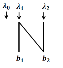
(a) N model

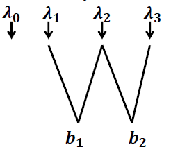
(b) W model

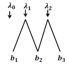
(c) M model

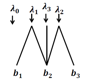
(d) M+1 model

Figure 1: The N, W, M, and M+1 model instances.

When there are $J=3$ slot types, the simplest nontrivial choice matrix is the M model instance in Figure 1(c) with

$$\Omega=\left(\begin{array}[]{lll}1&1&0\\ 0&1&1\\ \end{array}\right).$$

It turns out that in this case, the offering-all policy is not always optimal; rather, rationing of the versatile type-2 slot is needed. We define policy $\pi_{1}$ according to its offer set:

$$S^{\pi_{1}}(\mathbf{m}):=\left\{\begin{tabular}[]{ll}$\{1,3\}$&if $m_{1}>0$ and $m_{3}>0$,\\ $\bar{S}(\mathbf{m})$&otherwise.\end{tabular}\right.$$ (4)

So policy $\pi_{1}$ proposes to hold back on offering type-2 slots until either type-1 or type-3 slots are used up. We now formalize that one cannot do better than this.

Proposition 2.

For the M model instance, $\pi_{1}$ is optimal.

The intuition behind Proposition 2 is that blocking slot type 2 does not lead to any immediate loss of customer demand compared to offering it, while forcing early customers into less popular slot types (types 1 and 3). This preserves the popular (or, versatile) slots (type 2) for later arrivals, when slots run low. For convenience of discussion, we say a slot type is more popular (or, versatile) if this slot type is accepted by a superset of customer types compared to its counterpart.

Following from Proposition 2, we know that a versatile type 2 slot is at least as valuable as one of the other two less popular slot types at all times, for otherwise it would be better to offer type 2 slots but not offering the more valuable, less popular slot type. To be more specific, we have the following corollary.

Corollary 1.

In the M model instance, for either $j=1$ or 3 or both,

$$V_{n}(\mathbf{m}-\mathbf{e}_{2})\leq V_{n}(\mathbf{m}-\mathbf{e}_{j}),~{}\forall\mathbf{m}>0,~{}n\in\{1,\dots,N\}.$$ (5)

However, it is important to note that one of the two less popular slot types (1 and 3) may be strictly more valuable than the popular type 2. For example, for $\lambda_{1}=\lambda_{2}=0.5$, it is easy to verify that $V_{2}(2,1,0)=1.625<1.75=V_{2}(2,0,1)$. The reason here is the following. With $m_{1}=2$ and $n=2$, sufficient capacity is available for potential type 1 customer demand (i.e., at most 2 units). If $(m_{2},m_{3})=(1,0)$, the one unit of type 2 slot has a positive probability of being taken by a type 1 customer (which would be a waste); in contrast, if $(m_{2},m_{3})=(0,1)$, the one unit of type 3 slot can only be exclusively offered to type 2 customers (for whom no sufficient capacity is available), ant thus this is more efficient. This simple example shows that because of customers’ ability to (randomly) choose from their offer set, less popular slots may be more valuable than versatile slots due to resource imbalance. This observation implies that the (future) value of keeping a slot type cannot be viewed solely based on the number of accepting customer types, irrespective of the arrival probabilities or slot capacities. This complication renders the optimal policy for a general model instance quite complex, as we demonstrate now.

The next model instance that we focus on is the M+1 model instance shown in Figure 1(d), with choice matrix

$$\Omega=\left(\begin{tabular}[]{lll}1&1&0\\ 0&1&1\\ 0&1&0\end{tabular}\right).$$

Note that the only difference between the M+1 and M model instances is the additional customer type 3 that only accepts type 2 slots. It turns out that the simple, elegant form of the optimal policies in the previous cases does not carry over to the M+1 model instance.

To illustrate the complexity of the M+1 model instance, consider the case with $m_{1}=4$ and $n=5$. Figure 2 shows the unique optimal offer set, identified with $S\subset\{1,2,3\}$, as a function of $m_{2}$ and $m_{3}$. (For instance, if $S=\{1,3\}$, it means offering slot types 1 and 3 but not slot type 2.) Consider $\lambda_{1}=\lambda_{2}=0.1$, $\lambda_{3}=0.8$ (Figure 2(a)) or $\lambda_{1}=\lambda_{2}=0.475$, $\lambda_{3}=0.05$ (Figure 2(b)).

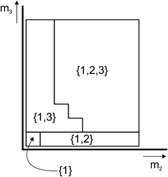
(a) $\lambda_{1}=\lambda_{2}=0.1$, $\lambda_{3}=0.8$

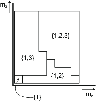
(b) $\lambda_{1}=\lambda_{2}=0.475$, $\lambda_{3}=0.05$

Figure 2: The optimal policy for an M+1 model instance, with $m_{1}=4$, $n=5$.

As discussed earlier, resource imbalance can make a less popular slot more valuable than a more popular one, which naturally would suggest an action of saving the less popular slot by only offering the versatile slot. Indeed, in Figure 2(b), we see that action $\{1,2\}$ can be the unique optimal action even when $\mathbf{m}>0$. This is true because $m_{3}$ is relatively small (equal to 1 or 2 in this case), while $m_{1}=4$ is ample given $n=5$ and the symmetric arrival rates of type 1 and type 2 customers. Blocking type 3 and offering the versatile type 2 earlier rather than later can help to resolve the resource imbalance by maximizing the total expected amount of type 2 slots taken by type 2 customers (and thus saving type 3 slots that can only serve type 2 customers for the future).

In addition, we see that the arrival rate now has a strong impact on the optimal policy, in contrast to the other cases we discussed so far: when $\lambda_{3}$ is large it is often optimal to include type 2 slots in the offer set, while for $\lambda_{3}$ small this is not the case. The reasoning here is that for $\lambda_{3}$ small the model is very close to the M model instance, for which we know it is optimal to save versatile type 2 slots for later in the booking process. However, not offering type 2 slots also implies turning away all type 3 customers, which explains why this slot type should be offered when $\lambda_{3}$ is large.

These observations we make on the M+1 model instance suggest that the optimal policy depends on the customer preference profiles, arrival rates and available slot capacity of the specific model instance under consideration. The optimal policy for a general model can be quite complex and have no straightforward structural properties. Thus, we shall focus our efforts on identifying simple scheduling policies that have performance guarantees and perform well in practice.

3.2 Asymptotically Optimal Policy

In this section, we construct a static randomized policy that is asymptotically optimal when we increase the system demand and capacity simultaneously. We first introduce the class of static randomized policies. At any decision epoch, there are altogether $2^{J}$ possible actions in terms of which slot types to offer. Here we use a binary vector to denote the offer set, with a 1 at position $j$ meaning that slot type $j$ is offered, and 0 otherwise. For example, we denote by the action of closing all slots as $\mathbf{w}^{1}:=(0,...,0)$, the $J$-dimensional zero vector, and the action of opening all slots as $\mathbf{w}^{2^{J}}:=(1,...,1)$, the $J$-dimensional one vector. We call the set of all $2^{J}$ $J$-dimensional 0-1 vectors as set $\mathcal{W}:=\{0,1\}^{J}$ and name the elements of the set as $\mathbf{w}^{1},\mathbf{w}^{2}...,\mathbf{w}^{2^{J}}$. Define $\mathcal{K}:=\{1,...,2^{J}\}$ as the action index set and so $\mathcal{K}$ and $\mathcal{W}$ have the same cardinality.

A policy $\pi^{p}$ is a static randomized policy if $\pi^{p}$ offers $\textbf{w}^{k}$ with some fixed probability $p_{k}$, independent of the system state and the time period. The class of static randomized policies contains all $\pi^{p}$’s such that the vector $\textbf{p}=\{p_{k}\}_{k=1}^{2^{J}}$ is a probability vector. For instance, the offering-all policy is a special case in this class with $p_{2^{J}}=1$ and $p_{k}=0$ for all $k\neq 2^{J}$.

We show that there exists a vector $\textbf{p}^{*}$ such that $\pi^{p^{*}}$ is asymptotically optimal when the demand and capacity are scaled up simultaneously. The choice of $p^{*}_{k}$ relies on the fluid model corresponding to the stochastic model (3) considered above, in which we can readily determine the optimal offering policy. We choose $p^{*}_{k}$ such that it represents the fraction of the time in which the action $\textbf{w}^{k}$ is used in a fluid model under optimal control. Below we construct this asymptotically optimal policy $\pi^{p^{*}}$ and defer more technical details to the Online Appendix.

3.2.1 Fluid Model

We first introduce our fluid model. To differentiate from the notation in the stochastic model formulation (3), we shall put the time index $n$ in parentheses, instead of as a subscript. Instead of discrete customers arriving in each slot, we represent a customer by a unit of fluid. In total one unit of demand arrives in each time period, a fraction $\lambda_{i}$ of which corresponds to customer type $i$. This fluid is distributed evenly among all available slots that are offered and accepted by the corresponding customer type.

For each $n=1,...,N$, the decision vector in the fluid model is $\mathbf{z}(n)=(z_{1}(n),...,z_{2^{J}}(n))$, which is a $2^{J}$ dimensional vector, each component $z_{k}(n)\in[0,1]$ representing the time during which action $k\in\mathcal{K}$ is being used in period $n$. Note that each action can be used for any fractional unit of time. Thus we require that

$$0\leq z_{k}(n)\leq 1,\forall k\in\mathcal{K},n=1,...N;$$ (6)

$$\sum_{k\in\mathcal{K}}z_{k}(n)=1,\forall n=1,...N.$$ (7)

Constraint (7) ensures that the total time spent on all possible actions (including the one that closes all slot types) in one period adds up to one.

Let $\boldsymbol{\tau}(n)=[\tau_{k,j}(n)]$ be a $2^{J}\times J$ matrix, each row of which corresponds to one of the $2^{J}$ possible actions. We use $\tau_{k,j}(n)$ to indicate the amount of time for which type $j$ slots are offered during the time when the $k$th action is taken in period $n$. We have that

$$\tau_{k,j}(n)=z_{k}(n)\mathbf{w}^{k}_{j},~{}~{}\forall k\in\mathcal{K},~{}j=1,2,\dots,J,~{}n=1,...N,$$ (8)

where $\mathbf{w}^{k}_{l}$ denotes the $l$th coordinate of vector $\mathbf{w}^{k}$. Constraint (8) is presented mainly to make the formulation clearer and easier to understand. It ensures that slot type $j$ can be open when action $k$ is chosen only if action $k$ offers slot type $j$. If action $k$ does not offer slot type $j$, then $\mathbf{w}^{k}_{j}=0$ and $\tau_{k,j}(n)$ is zero by (8). Let $\mathcal{J}_{k}=\{j:\mathbf{w}^{k}_{j}=1,~{}j=1,2,\dots,J.\}$ be the full set of slot types offered by action $k$. Note that (8) implies that

$$\tau_{k,j_{1}}(n)=\tau_{k,j_{2}}(n),~{}~{}\forall k\in\mathcal{K},~{}n=1,...N,~{}j_{1},j_{2}\in\mathcal{J}_{k}.$$

That is, if an action $k$ offers multiple slot types, the offering durations of these slot types are the same.

Let $y_{i,j}(n)$ denote the amount of type $j$ slot’s capacity filled by type $i$ customers during period $n$ and $\mathcal{K}_{j}=\{s:\mathbf{w}^{s}_{j}=1,s\in\mathcal{K}\}$ be the index set of actions that offer type $j$ slots. If $\Omega_{i,j}=1$,

$$y_{i,j}(n)=\sum_{k\in\mathcal{K}_{j}}\tau_{k,j}(n)\cdot\frac{\lambda_{i}}{\sum_{l=1}^{J}\min\{\Omega_{i,l},\mathbf{w}^{k}_{l}\}},~{}i=1,2,\dots,I,~{}j=1,2,\dots,J,~{}n=1,...,N;$$ (9)

and otherwise if $\Omega_{i,j}=0$, then

$$y_{i,j}(n)=0,~{}i=1,2,\dots,I,~{}j=1,2,\dots,J,~{}n=1,...,N.$$ (10)

Note that all terms in (9) except $\tau_{k,j}(n)$’s are constants and therefore (9) as a set of constraints for the optimization problem is linear in the decision variables $\tau_{k,j}(n)$.

Let $M_{j}(t)$ be the amount of type $j$ slots left with $t$ time periods to go and let $Z_{N}(\mathbf{m})$ be the optimal amount of (fluid) customers served with initial capacity vector $\mathbf{m}$ and $N$ periods to go. The goal is to choose $z_{k}(n)$ (and $\tau_{k,j}(n)$) in order to solve for

$$Z_{N}(\mathbf{m})=\max\sum_{n=1}^{N}\sum_{j=1}^{J}\sum_{i=1}^{I}y_{i,j}(n),$$ (P1)

s.t. (6), (7), (8), (9), (10), and

$$M_{j}(N)=m_{j}, j=1,2,\dots,J,$$ (11)

$$M_{j}(n-1)=M_{j}(n)-\sum_{i=1}^{I}y_{i,j}(n), j=1,2,\dots,J,~{}n=1,...,N,$$ (12)

$$M_{j}(n)\geq 0, j=1,2,\dots,J,~{}n=0,1,...,N-1.$$ (13)

In (P1), constraint (11) specifies the initial capacity vector, (12) updates the capacity vector for each period, and (13) ensures that all slot types have nonnegative capacity throughout. We remark that in our formulation, control can be exerted anytime continuously throughout the horizon but the system is observed only at discrete time epochs $0,1,2,\dots,N$ to match the stochastic model formulation (3).

3.2.2 Choice of $\mathbf{p}^{*}$

Let $p^{*}_{k}$ be the fraction of the time in which the optimal policy chooses action $k$ in the fluid model (P1). That is,

$$p^{*}_{k}=\frac{\sum_{n=1}^{N}z^{*}_{k}(n)}{N},$$ (14)

where $z^{*}_{k}(n)$ is the optimal solution to (P1). We now translate this optimal policy for the fluid model to our original discrete and stochastic setting by defining a policy $\pi^{p^{*}}$ such that in each period $n$, this policy offers $\textbf{w}^{k}$ with probability $p^{*}_{k}$, independent of everything else.

The intuition behind choosing $\mathbf{p}^{*}$ as the offering probability vector is that if we scale up the system demand (i.e., $N$) and capacity (i.e, $\mathbf{m}$) in the stochastic model, using $\pi^{p^{*}}$ makes the proportion of total customer demand going to each slot type in the stochastic model approximately matches that in the fluid model. Thus, the total fill counts in the stochastic model is similar to that of the fluid model. Because the fluid model is a deterministic model which provides an upper bound on the objective value of the stochastic model (more on this below), we know that $\mathbf{p}^{*}$ is (close to) optimum in the stochastic model as the system becomes large. We formalize this intuition in the next section.

3.2.3 Main Result

Consider a sequence of problems indexed by $K=1,2,3\dots$. The problems in this sequence are identical except that for the $K$th problem, the number of total periods is $NK$ and the capacity vector is $\textbf{m}K$. We call the problem instance with $K=1$ as the base problem instance. Let $V_{n}^{\pi^{p}}(\cdot)$ be the total expected number of slots filled under a policy $\pi^{p}$ with the offering probabiity vector $\mathbf{p}$ in the stochastic model. The main result is shown in the following theorem.

Theorem 1.

(i) $K^{-1}V_{NK}(\textbf{m}K)\leq K^{-1}Z_{NK}(\mathbf{m}K)=Z_{N}(\mathbf{m}),~{}\forall\mathbf{m}\geq 0,~{}K=1,2,3,\dots$;
(ii) $\lim_{K\rightarrow\infty}K^{-1}V^{\pi^{p^{*}}}_{NK}(\textbf{m}K)=Z_{N}(\mathbf{m})$.

Recall that $V_{n}(\cdot)$ is the optimal value of the stochastic model defined in (3). Thus Theorem 1(i) says that the “normalized” optimal value of the non-sequential offering stochastic model (i.e., the original value divided by $K$) is bounded from above by that of the corresponding fluid model, and that the normalized objective value of the fluid model is the same as the objective value of the base fluid model with $K=1$. Theorem 1(ii) states that as the system grows large, the normalized objective value in the stochastic system under policy $\pi^{p^{*}}$ converges to this constant upper bound, and thus $\pi^{p^{*}}$ is asymptotically optimal.

The proof of Theorem 1 entails a few key steps which are outlined below (full details can be found in the Online Appendix). We first show that the optimal objective value of the fluid model is an upper bound of the optimal value of the stochastic model, i.e., $Z_{N}(\mathbf{m})\geq V_{N}(\mathbf{m})$, for any given set of model parameters. Then, based on any static randomized policy $\pi^{p}$, we construct a lower bound for $V_{n}^{\pi^{p}}(\cdot)$, and this lower bound is naturally a lower bound for the optimal value of the stochastic model $V_{N}(\mathbf{m})$ (because $\pi^{p}$ is not necessarily optimal). Finally, we show that when $p$ is chosen as $p^{*}$ defined in (14), the normalized lower bound converges to $Z_{N}(\mathbf{m})$ when the system grows in both demand and capacity. Thus, $\pi^{p^{*}}$ is asymptotically optimal.

Our findings build upon the early classic results in the revenue management literature, which show that allocation policies arising from a single linear program make the normalized total expected revenue converge to an upper bound on the optimal value (Cooper 2002). Our results are different and new in several important aspects. The model in Cooper (2002) can designate/allocate a particular product (slot) type upon a customer arrival (because he assumes that customer preference is known upon arrival), while our model offers multiple product (slot) types for customers to choose from (because the customer preference is not known). Using the offer set as a decision in the model creates significant new challenges. First of all, our fluid model formulation needs to explicitly take care of customer choice processes and is much more complicated than that in Cooper (2002). Leveraging the fluid model formulation, the asymptotically optimal policy in Cooper (2002) accepts customer requests up to some customer type-specific thresholds, because the optimal solution in Cooper’s fluid model prescribes such thresholds for each customer type. As a result, Cooper’s asymptotic policy leads to a closed-form expression for each type of the customer demand served, allowing him to directly show that the normalized demand served converges in distribution to a constant which matches the optimal fluid model decision. However, due to customer choices, our fluid model cannot give rise to such a simple policy. Our fluid model informs the optimal duration in which a particular offer set is used, and we use this information to construct our policy which has a completely different form compared to Cooper’s policy. As we cannot control the exact product (slot) type in an offer set that will be chosen by an arriving customer, we do not have a closed-form expression as in Cooper (2002) for the total demand that goes into each product (slot) type and eventually gets served. To deal with this difficulty, we construct a (very) tight lower bound on the objective value and show that this lower bound, after being normalized, converges to the optimal objective value of the fluid model. The idea of our proof may be useful to identify effective approximate policies in other capacity management contexts when the manager cannot directly control the product a customer may pick.

3.3 Constant Performance Guarantee of the Offering-all Policy

In this section, we focus on a simple scheduling policy: the offering-all policy. Let $\pi_{0}$ represent this policy, so the offer set under $\pi_{0}$ is the full set of all slot types, irrespective of the period $n$. Note that the effective offer set at state $\mathbf{m}$ is $\bar{S}(\mathbf{m})$. That is, when customers arrive, they only consider those slot types with positive capacity when making a choice. We denote by $V_{n}^{\pi_{0}}(\mathbf{m})$ the expected fill count attained by applying the offering-all policy $\pi_{0}$ throughout. Indeed, this simple policy has a constant performance guarantee that states that for any set of parameters, the offering-all policy $\pi_{0}$ achieves at least half of the optimal fill count.

Theorem 2.

For any $\Omega$, $n$, and $\mathbf{m}$, $V_{n}(\mathbf{m})\leq 2V_{n}^{\pi_{0}}(\mathbf{m})$.

It is worth noting that Theorem 2 in fact holds more broadly for all so-called myopic policies, which at each period offer a set maximizing the expected number of filled slots for that period. Myopic policies, however, do not have to offer all slot types in all periods. For instance, offering slot types 1 and 3 in the M model instance would constitute a myopic policy.

Performance guarantee results on myopic policies exist in various dynamic optimization settings, and a ratio of 2 is often the best provable performance bound; see, e.g., Mehta (2013), Chan and Farias (2009). While this performance bound may seem a little loose, we shall see empirically in Section 5.1 that the offering-all policy performs very well and much better than this lower bound; in finite regimes, the offering-all policy also seems to perform better than the asymptotically optimal policy constructed in Section 3.2.

4 Sequential Offering

We now present our second scheduling paradigm, which allows the scheduler to offer multiple sets of slots sequentially. Recall that this way of offering slots may represent for instance web-based scheduling where available slots are not revealed simultaneously, as well as telephone-based scheduling. Intuitively, having the scheduler offer slots sequentially instead of all at once will be able to steer customers into selecting more favorable slots from the perspective of system optimization. The question we address in this section is then how many and what sets of slots to offer in order to maximize the fill rate. We start by introducing the sequential offering model next.

4.1 Model Outline

Upon customer arrival, the scheduler chooses a $K$, $1\leq K\leq J$, and sequentially presents the customer with $K$ mutually exclusive subsets $S_{1}$, $S_{2}$,$\dots$, $S_{K}\subseteq\bar{S}(\mathbf{m})$. We denote this action as $\mathbf{S}:=S_{1}-S_{2}-\dots-S_{K}$. Denote by $\mathscr{S}(\mathbf{m})$ the set of all possible such actions at state $\mathbf{m}$, and by $I_{k}(\mathbf{S}):=\{i:\sum_{j\in S_{k}}\Omega_{ij}\geq 1,i\notin\cup_{l=1}^{k-1}I_{l}(\mathbf{S})\}$, $k=1,...,K$, the set of customer types who do not accept any slot from the first $(k-1)$ offer sets but encounter at least one acceptable slot in $S_{k}$. So $I_{k}(\mathbf{S})$ represents the set of customers who, given sequential offering $\mathbf{S}$, accept some slot upon arrival into the system. Moreover, the slot chosen by these customers belongs to the $k$th offer set $S_{k}$. The probability that slot type $j$ is chosen under action $\mathbf{S}$ may then be written as $q_{j}(\mathbf{S}):=\sum_{k=1}^{K}\sum_{i\in I_{k}(\mathbf{S})}\lambda_{i}q_{ij}(S_{k})$, with $q_{ij}(\cdot)$ as in (1). The assumption that the sets $S_{1},S_{2},\dots,S_{K}$ are mutually exclusive is made from a practical rather than mathematical standpoint: there is simply no reason to offer the same slot type in two or more sets, because the customer will book a slot as soon as she is offered a set with at least one acceptable slot. Thus only the first set in which such a slot is included is relevant.

For ease of presentation, we still use $V_{n}(\mathbf{m})$ to denote the expected maximum number of slots that can be booked with $\mathbf{m}$ slots available and $n$ periods to go in this section. For an action $\mathbf{S}$, we let $\bigcup\mathbf{S}:=\bigcup_{i=1}^{K}S_{i}$ denote the set of all slot types offered throughout action $\mathbf{S}$. Then, for the sequential offering model, we have

$$V_{n}(\mathbf{m})=\max_{\mathbf{S}\in\mathscr{S}(\mathbf{m})}\left[\sum_{j\in\bigcup\mathbf{S}}q_{j}(\mathbf{S})(1-\Delta_{n-1}^{j}(\mathbf{m}))\right]+V_{n-1}(\mathbf{m}),\mbox{~{}~{}for~{}}n=N,N-1,...,1,$$ (15)

where $V_{0}(\cdot)=0$ and $\Delta_{n-1}^{j}(\mathbf{m}):=V_{n-1}(\mathbf{m})-V_{n-1}(\mathbf{m}-\mathbf{e}_{j})$ denotes the marginal benefit due to the $m_{j}$th unit of slot type $j$ at period $n-1$. We observe that both the transition probability $q_{j}(\mathbf{S})$ and the set of feasible actions $\mathscr{S}(\mathbf{m})$ are much more complicated than their counterparts in the non-sequential model.

The sequential offering setting can be viewed as a generalization of non-sequential scheduling to any number $K\geq 1$ of offer sets. Consequently, it stands to reason that the offering-all policy will not perform well in the sequential setting, as this would limit the scheduler to a single offer set ($K=1$). We indeed numerically confirm this conjecture in Section 5.3. Note that, in contrast to the non-sequential case, an offering-all policy is unlikely to be used in a practical setting such as telephone scheduling (because it would take too much time for the scheduler to go over every possible appointment option). In the online setting, there is a way to take advantage of sequential offerings by redesigning the customer interface that releases information sequentially.

To provide a roadmap of analyzing the sequential model, we summarize our key findings in this section as follows.

• We first consider a general setting and derive various structural results that provide more insights; in particular, we show that it is optimal to offer slot types one by one.

• For a large class of problem instances with nested preference structures (to be discussed later), we derive a closed-form optimal sequential offering policy.

• For problem instances not in this class, we develop a simple and highly effective heuristic based on the idea of balanced resource use and fluid models.

• We prove that the optimal sequential offering does as well as in the non-sequential case where the scheduler has full information on the customer type upon arrival; we argue that this equivalence allows us to apply the idea of sequential offering in various interactive scheduling contexts.

4.2 Results for the General Sequential Offering Model

We now present some properties of the sequential model with general choice matrices. First, we derive some structural properties of the value function.

Lemma 1.

The value function $V_{n}(\mathbf{m})$ satisfies:
(i) $0\leq V_{n+1}(\mathbf{m})-V_{n}(\mathbf{m})\leq 1$, $\forall\mathbf{m}\geq 0$, $\forall n=1,2,\dots,N-1$; and
(ii) $0\leq V_{n}(\mathbf{m}+\mathbf{e}_{j})-V_{n}(\mathbf{m})\leq 1$, $\forall\mathbf{m}\geq 0$, $\forall n=1,2,\dots,N$.

Part (ii) of Lemma 1 implies that $V_{n}(\mathbf{m}+\mathbf{e}_{j})\leq V_{n}(\mathbf{m})+1$, i.e., it is better to have a slot booked now rather than saving it for future. Therefore, in the context of sequential offering, it is better to keep offering slots if none has been taken so far. This is formalized in the following result, which shows that there exists an optimal sequential offering policy that exhausts all available slot types in each period.

Lemma 2.

For any $\Omega$, $\mathbf{m}$, and $n$, there exists an optimal action $\mathbf{S}^{*}$ such that $\bigcup\mathbf{S}^{*}=\bar{S}(\mathbf{m})$.

Building upon Lemma 2, we are able to characterize the structure of an optimal sequential offering policy, described in the theorem below.

Theorem 3.

Let $\mathbf{m}>0$ be the system state at period $n\geq 1$, and let $j_{1},j_{2},...,j_{J}$ be a permutation of $1,2,...,J$ such that $V_{n-1}(\mathbf{m}-\mathbf{e}_{j_{k}})\geq V_{n-1}(\mathbf{m}-\mathbf{e}_{j_{k+1}})$, $k=1,2,\dots,J-1$. Then the action $\{j_{1}\}-\dots-\{j_{J}\}$ is optimal.

Theorem 3 implies that there exists an optimal policy that offers one slot type at a time. More importantly, this result shows a specific optimal offer sequence based on the value function to go. To understand this, recall that $V_{n-1}(\mathbf{m})-V_{n-1}(\mathbf{m}-\mathbf{e}_{j})$ can be viewed as the value of keeping the $m_{j}$th type $j$ slot from period $n-1$ onwards. As all customers bring in the same amount of reward, it benefits the system the most if an arrival customer can be booked for the slot type with the least value to keep, i.e., the slot type with the largest $V_{n-1}(\mathbf{m}-\mathbf{e}_{j})$.

Even if the scheduler does not know the exact customer type, following the optimal offer sequence described in Theorem 3 ensures that the arriving customer takes the “least valuable” slot (as long as there is at least one acceptable slot remaining). Indeed, matching customers with slots in this way would be the best choice for the scheduler, even if she had perfect information about customer type, i.e., she knew exactly the customer type upon arrival. Following this rationale, our next result shows an interesting and important correspondence between (i) the sequential offering without customer type information and (ii) the non-sequential offering with perfect customer type information. To distinguish these two settings, we let $V^{s}_{n}(\mathbf{m})$ and $V^{f}_{n}(\mathbf{m})$ represent the value functions for settings (i) and (ii), respectively, in the next theorem.

Theorem 4.

$V^{s}_{n}(\mathbf{m})=V^{f}_{n}(\mathbf{m})$, $\forall~{}\mathbf{m}\geq 0,~{}n=0,1,2,\dots,N$.

Theorem 4 suggests that the optimal sequential offering can fully exploit the value of customer type information; however, it does not imply that it can fully elicit customer type. Specifically, optimal sequential offering happens to result in the same system state changes as if the scheduler had full information about customer type, but does not let the scheduler know exactly the customer type (see Remark 2 in Section 4.4). Theorem 4 suggests that sequential offering is a useful operational mechanism to improve the scheduling efficiency in the absence of customer type information. Our numerical experiments in Section 5 confirm and quantify such efficiency gains.

4.3 Optimal Sequential Offering Policies

In this section we fully characterize the optimal sequential offering policy for a large class of choice matrix instances, which include the N, M and M+1 model instances (see Figure 1). To this end, let $I(j)$ be the set of customer types who accept slot type $j$, i.e., $I(j)=\{i=1,2,\dots,I:\Omega_{ij}=1\}$, $\forall j=1,2,\dots,J$. It makes intuitive sense that if $I(j_{1})\subset I(j_{2})$, then slot type $j_{2}$ is more valuable than $j_{1}$, and thus slot type $j_{1}$ should be offered first. Combining this observation with Theorem 3 could then help us to design an optimal policy. Let us first introduce a specific class of model instances.

Definition 1.

We say that a model instance characterized by $\Omega$ is nested if for all $j_{1},j_{2}=1,2,\dots,J$ and $j_{1}\neq j_{2}$, one of the following three conditions holds: (i) $I(j_{1})\cap I(j_{2})=\emptyset$, (ii) $I(j_{1})\subset I(j_{2})$, or (iii) $I(j_{1})\supset I(j_{2})$.

Note that not all model instances are nested. One simple example is the W model instance from Figure 1(b), where $I(1)=\{1,2\}$ and $I(2)=\{2,3\}$. None of the conditions (i)-(iii) from Definition 1 hold in this case for $j_{1}=1$ and $j_{2}=2$. However, it is readily verified that the N, M and M+1 model instances are all nested.

Remark 1.

The concept of a nested model instance is related to the star structure considered in the previous literature on flexibility design; see, e.g., Akçay et al. (2010). Consider a system with a certain number of resource types (corresponding to slot types in our context), which can be used to do jobs of certain types (customer types in our context). A star flexibility structure is one such that there are specialized resource types, one for each job type, plus a versatile resource type that can perform all job types. The nested structure generalizes the star structure.

It turns out that we can fully characterize an optimal policy for nested model instances as follows.

Theorem 5.

Suppose $\Omega$ is nested, any policy that offers slot type $j_{1}$ before offering slot type $j_{2}$ for any $j_{1},~{}j_{2}$ such that $I(j_{1})\subset I(j_{2})$ is optimal.

Theorem 5 proposes to offer nested slot types in an increasing order of the accepting customer types. Note that when two slot types are mutually exclusive (i.e., $I(j_{1})\cap I(j_{2})=\emptyset$), the order in which they are offered is irrelevant, since customers that would select a slot from one set could never from the other. To give some specific examples, we can fully characterize the optimal policy for the N, M and M+1 model instances using Theorem 5.

Corollary 2.

For the N model instance and any $n$ and $\mathbf{m}$, an optimal sequential offering policy is to offer $\mathbf{S}=\{1\}-\{2\}$.

Corollary 3.

For the M and M+1 model instances and any $n$, an optimal sequential offering policy is to offer

$$\mathbf{S}=\left\{\begin{array}[]{ll}\{1,3\}-\{2\},&{\rm~{}if~{}}m_{1},m_{2},m_{3}\geq 1,\\ \{1\}-\{2\},&{\rm~{}if~{}}m_{3}=0,\\ \{3\}-\{2\},&{\rm~{}if~{}}m_{1}=0.\end{array}\right.$$

4.4 Beyond Nested Model Instances

While Theorem 5 solves a large class of the sequential model instances, not all instances have a nested structure. In this section, we analyze the W model instance (see Figure 1) to glean some insights into the instances which are not nested.

To analyze the W model instance, one can formulate an MDP with three possible actions: $\{1,2\}$, $\{1\}-\{2\}$, and $\{2\}-\{1\}$ (and the corresponding actions at the boundaries). However, there exist no straightforward offering orders for slot types, and the optimal sequential policy turns out to be state dependent. Specifically, we find that the optimal policy is a switching curve policy: with the availability of one type of slots held fixed, it is optimal to offer the other type of slots first as long as there is a sufficiently large amount of such slots left.

Figure 3 illustrates the optimal actions for the W model instance at different system states with $\mathbf{\lambda}=(0.2,0.5,0,3)$ and $n=6$. The symbols “0”, “1”, “2”, “12” and “21” correspond to the actions of offering nothing, offering type 1 slots only, offering type 2 slots only, offering type 1 slots and then type 2 slots, and offering type 2 slots and then type 1 slots, respectively. The optimal actions at boundary are obvious. In the interior region of the system states, we can clearly see the switching curve structure. For instance, when the system state is $(3,3)$, it is optimal to offer $\{1\}-\{2\}$. When the number of type 2 slots increase to 4, then it is optimal to offer $\{2\}-\{1\}$.

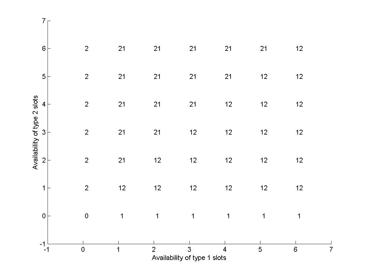
Figure 3: Structure of the optimal policy under W model instance with sequential offers.

The intuition behind this is different from that of the model instances considered above where customer preferences are nested (e.g., the N, M and M+1 model instances). In the W model instance, type 1 (3 resp.) customers only accept type 1 (2 resp.) slots; but type 2 customers accept both types of slots. If there are relatively more type 1 slots than type 2 slots, then it makes more sense to “divert” type 2 customers to choose type 1 slots, thus saving type 2 slots only for type 3 customers. Accordingly, the switching curve policy stipulates that type 1 slots to be offered first, ensuring that type 2 customers if any will pick type 1 slots. The intuition above is formalized in the proposition below.

Proposition 3.

Consider the W model instance with sequential offers. Given $m_{2}$, if there exists an $m_{1}^{*}$ such that the optimal action at state $(m_{1}^{*},m_{2})$ is $\{1\}-\{2\}$, then $\forall\mathbf{m}\in\{(m_{1},m_{2}),m_{1}\geq m_{1}^{*}\}$, the optimal action is $\{1\}-\{2\}$. Similarly, given $m_{1}$, if there exists an $m_{2}^{*}$ such that the optimal action at state $(m_{1},m_{2}^{*})$ is $\{2\}-\{1\}$, then $\forall\mathbf{m}\in\{(m_{1},m_{2}),m_{2}\geq m_{2}^{*}\}$, the optimal action is $\{2\}-\{1\}$.

Remark 2.

In Section 4.3, we state that sequential offering may not fully reveal exact customer types, but allows the system to evolve in the same optimal way as if the scheduler knew exactly the customer type. We use the W model instance to illustrate this point. Consider the W model instance with non-sequential offers and the scheduler knows the exact type of arriving customers. Suppose the optimal action is to offer $\{1\}$ when type 1 or type 2 customers arrive; and to offer $\{2\}$ when type 3 customer arrives. Now, in a sequential offering model where the scheduler does not know the exact type of arriving customers, the scheduler would have offered $\{1\}$-$\{2\}$ to any arriving customer. If we encountered type 1 or 2 customers, type 1 slot would be taken, but we do not know the exact type of this customer (we know she must be either type 1 or type 2 though); if type 3 customer arrived, she would reject type 1 slot, but take type 2 slot. In this way, the system evolves as if the scheduler had perfect information on customer type.

The structural properties of the optimal policy described in Proposition 3 are likely the best we can obtain for the W model instance; the exact form of the optimal policy depends on model parameters and the system state, much like with the M+1 model instance in the non-sequential case. If customer preference structures become more complicated, it is very difficult, if not impossible, to develop structural properties for the optimal sequential offering policy. Thus, for model instances that do not satisfy the conditions of Theorem 5, we propose an effective heuristic below.

4.5 The “Drain” Heuristic

If customer preferences are not nested, the analysis of the W model instance suggests that the optimal policy is to offer slots with more capacity relative to its customer demand. Inspired by this observation and using the idea of fluid models, we propose the following heuristic algorithm which aims to “drain” the abundant slot type first followed by less abundant ones. This heuristic aims to have all slot types emptied simultaneously, thus maximizing the fill rate. That is, this heuristic tries to “balance” the resource use. Specifically, the drain algorithm works in the following simple way. At period $n$ and for each slot type $j\in\bar{S}(\mathbf{m})$, we calculate

$$I_{j}:=\frac{m_{j}}{n\sum_{i=1}^{I}\lambda_{i}\frac{\Omega_{ij}}{\sum_{k\in\bar{S}(\mathbf{m})}\Omega_{ik}}}.$$ (16)

Note that $\frac{\Omega_{ij}}{\sum_{k=1}^{J}\Omega_{ik}}$ represents the share of type $i$ customers who will choose type $j$ slots, assuming all available slot types are offered simultaneously. Taking expectation with respect to the customer type distribution and multiplying by $n$, the number of customers to come, the denominator of (16) can be viewed as the expected load on type $j$ slots in the next $n$ periods. As a result, the index $I_{j}$ can be regarded as the ratio between capacity left and “expected” load.

The drain algorithm is then to calculate all $I_{j}$s at the beginning of each period, and to offer slots in decreasing order of the $I_{j}$. The algorithm calls for offering slot types with larger $I_{j}$ first, as these slot types have relatively more capacity compared to demand. In other words, a slot type with a larger $I_{j}$ is likely to have a smaller marginal value to keep, and thus can be offered earlier. We could of course safely remove $n$ in the definition of $I_{j}$, and obtain the exact same order of slots. However, we leave $n$ in the denominator of (16) because this allows us to interpret $I_{j}$ as the ratio between capacity left and “expected” number of requests. Based on this interpretation, it is clear that this heuristic aims to have all slot types emptied simultaneously, thus maximizing the fill rate. We will test the performance of this algorithm in Section 5.2.

4.6 Applications to Interactive Scheduling

In Sections 3 and 4 we discuss two different models of customer-scheduler interactions in the appointment booking practice. In one model, the scheduler makes a one-shot offering, and in the other, the scheduler enjoys the full flexibility of sequential offering. The appointment booking process, however, can fall in between these two models in terms of the degree to which the customer preference information is collected and used during the interaction between the scheduler and each customer. Such interactions may be present both in a traditional setting with human interaction (e.g., a customer, after being offered an appointment at 8am by a receptionist, may indicate that none of the morning slots are acceptable) or fully digital (e.g., the Partners HealthCare Patient Gateway online booking website allows patients to indicate their acceptable time slots upfront).

When additional customer preference information is gathered during the appointment booking process, the scheduler can still follow the optimal list of slot types $\{j_{1}\}-\dots-\{j_{J}\}$ obtained from Theorem 3, but simply skip all slots known to be unacceptable, either up front or dynamically as additional information is collected. This offering strategy is still optimal because it would end up with the same system state compared to not skipping those slots indicated as unacceptable before or during the booking process (e.g., directly declared by the customer) and thus give the exact same fill count that can be obtained if the scheduler had full information about the customer type (see Theorem 4). Recall that the order of $\{j_{1}\}-\dots-\{j_{J}\}$ can be readily obtained with nested customer preferences (Theorem 5), or otherwise an approximate order can be easily formed by the drain heuristic (16).

Although outside the scope of this paper, these considerations on interactive scheduling raise various issues related to the tradeoff between obtaining the best fill rate and providing a convenient experience to the customer. For instance, the scheduler may want to limit the number of sets offered to the customer to provide a smooth user experience. In light of Theorem 3, one potential idea for future study is to group slot types based on the order of $\{j_{1}\}-\dots-\{j_{J}\}$.

5 Numerical Results

In the last two sections, we consider non-sequential offering and sequential offering. For each setting, we derive optimal or near-optimal booking policies. In this section, we run extensive numerical experiments to test and compare these policies and the two scheduling paradigms.

We organize this section as follows. Section 5.1 and Section 5.2 discuss the performance of the offering-all policy in the non-sequential model and of the drain heuristic in the sequential model, respectively. We demonstrate that these two algorithms obtain fill rates that are remarkably close to that of the respective optimal policies, and therefore can serve as simple, effective heuristics for practical use. Section 5.3 compares the differences in the expected fill rate under the non-sequential and sequential offering models, where this difference represents the “value” of sequential offering. Specifically, we evaluate the differences between the optimal policies and those between the heuristics. The former represent the “theoretical” value of sequential offering compared to non-sequential offering, while the latter can be thought of as the “practical” value if practitioners adopt the heuristics mentioned above for each setting. Finally, Section 5.4 extends our scheduling policies to a multi-day rolling horizon setting and demonstrates that the insights obtained from our analysis remain valid in this setting.

5.1 Performance of the Offering-all Policy

We start our evaluation of the offering-all policy in two specific model instances considered above: M and M+1 model instances. (We need not to evaluate the offering-all policy in the N and W model instances because the offering-all policy is optimal there.) Here we use backward induction to determine the expected performance of the optimal policy $\pi_{1}$, and compare it through simulation to that of the offering-all policy $\pi_{0}$. To this end we simulate the offering-all policy for 1000 days. The performance metric of interest is the percentage optimality gap defined as $(u_{g}-u_{o})/u_{o}\times 100\%$, where $u_{o}$ is the expected fill count of the optimal policy and $u_{g}$ is the average fill count over 1000 simulated days under the offering-all policy.

Table 1 summarizes the statistics on the optimality gap of the offering-all policy in the M model instance. For each $N=20,30,40,50$, we evaluate the maximum, average and median optimality gap over all possible initial capacity vectors $(b_{1},b_{2},b_{3})\in\mathbb{Z}_{+}^{3}$ such that $b_{j}\geq 0.2N,~{}\forall j$ and $b_{1}+b_{2}+b_{3}=N$. The number of initial capacity vectors considered for each $N$ is shown as the number of scenarios in the second column of Table 1. In general, the optimality gap of the offering-all policy in the M model instance is relatively small ($\approx 3-4\%$) and is not sensitive to model parameters.

Table 1: Optimality gap of the offering-all policy in the M model instance.

$N$	$\#$ of	$(\lambda_{1},\lambda_{2})=(1/2,1/2)$			$(\lambda_{1},\lambda_{2})=(1/3,2/3)$			$(\lambda_{1},\lambda_{2})=(1/4,3/4)$
	Scenarios	Max	Average	Median	Max	Average	Median	Max	Average	Median
$20$	45	-4.4%	-3.6%	-3.6%	-4.1%	-3.3%	-3.3%	-3.6%	-2.9%	-3.0%
$30$	91	-4.8%	-3.7%	-3.8%	-4.5%	-3.5%	-3.5%	-3.8%	-3.1%	-3.2%
$40$	153	-5.1%	-3.8%	-3.8%	-4.7%	-3.6%	-3.6%	-4.0%	-3.2%	-3.3%
$50$	231	-5.3%	-3.8%	-3.8%	-4.8%	-3.7%	-3.7%	-4.1%	-3.3%	-3.4%

Table 2 shows the optimality gap statistics for the M+1 model instance, and the setup of this table is similar to Table 1. When $\lambda_{3}$ is small, the M+1 model instance is very similar to the M model and thus the optimality gaps of the offering-all policy are similar to those observed in Table 1. As $\lambda_{3}$ increases the performance of the offering-all policy improves, since offering-all becomes more likely to be optimal.

Table 2: Optimality gap of the offering-all policy in the M+1 model instance.

$N$	$\#$ of	$(\lambda_{1},\lambda_{2},\lambda_{3})=(9/20,9/20,1/10)$			$(\lambda_{1},\lambda_{2},\lambda_{3})=(2/5,2/5,1/5)$			$(\lambda_{1},\lambda_{2},\lambda_{3})=(3/10,3/10,2/5)$
	Scenarios	Max	Average	Median	Max	Average	Median	Max	Average	Median
$20$	45	-3.1%	-2.0%	-1.9%	-2.0%	-1.1%	-0.9%	-0.7%	-0.3%	-0.2%
$30$	91	-3.4%	-2.1%	-2.0%	-2.3%	-1.1%	-1.0%	-0.8%	-0.3%	-0.2%
$40$	153	-3.7%	-2.1%	-2.0%	-2.5%	-1.2%	-1.0%	-0.8%	-0.2%	-0.1%
$50$	231	-3.9%	-2.2%	-2.0%	-2.6%	-1.2%	-1.0%	-0.8%	-0.2%	-0.1%

To evaluate the performance of the offering-all policy in settings beyond these two simple instances, we carry out an extensive numerical study using randomly generated customer preference matrices. Fixing the number of slot types $J$, there are $2^{J}$ different possible customer types, including those that accept no slots at all. By allowing any possible combination of these customer types, there could be $2^{2^{J}}-1$ possible preference matrices (excluding the empty matrix). In order to test the performance of offering-all in a robust and yet computationally tractable manner, we compare its performance among many randomly generated such preference matrices.

We also vary the arrival probability vector $\boldsymbol{\lambda}=(\lambda_{1},\dots,\lambda_{I})$ for each preference matrix. In particular, we test three possible vectors: $\boldsymbol{\lambda}^{(1)}$ such that $\lambda^{(1)}_{i}=1/I$, $\boldsymbol{\lambda}^{(2)}$ such that $\lambda^{(2)}_{i}=2(I+i-2)/(3I^{2}-3I)$ and $\boldsymbol{\lambda}^{(3)}$ with $\lambda^{(3)}_{i}=2(I+3i-4)/(5I^{2}-5I)$. In all three cases the $\lambda_{i}$’s add up to one. For $\boldsymbol{\lambda}^{(2)}$ and $\boldsymbol{\lambda}^{(3)}$, $\lambda_{1}$ is the largest, and each successive $\lambda_{i}$ is smaller by a factor 2 or 4, respectively. Note that the value of $I$ depends on the randomly generated preference matrix, and may vary from $I=1$ (since we exclude the empty matrix) to the maximum number of customer types.

Our results are summarized in Table 3, where we show the optimality gap of the offering-all policy. We compute the performance of offering-all through simulation as before, and the performance of the optimal policy through backward induction. We fix $J$ and $N$, and then generate the number of random instances indicated in the table (‘number of instances’). For each instance we also vary the initial capacity vectors similar to what was done for Tables 1 and 2 (‘number of scenarios’). Fixing the structure of the arrival rate vector, we then report the maximum, average and median optimality gap over all instances and scenarios. It is clear from this table that the offering-all policy continues to do very well, and the average gap with the optimal policy is around $0.5\%$ throughout, independent of the size of the matrix and the arrival rates.

Table 3: Optimality gap of the offering-all policy for random network instances.

$J$	$N$	$\#$ of	$\#$ of	$\boldsymbol{\lambda}=\boldsymbol{\lambda}^{(1)}$			$\boldsymbol{\lambda}=\boldsymbol{\lambda}^{(2)}$			$\boldsymbol{\lambda}=\boldsymbol{\lambda}^{(3)}$
		Instances	Scenarios	Max	Average	Median	Max	Average	Median	Max	Average	Median
3	10	100	36	3.9%	0.2%	0.0%	3.9%	0.2%	0.0%	3.7%	0.3%	0.0%
	20	80	120	4.6%	0.3%	0.1%	4.6%	0.3%	0.1%	5.1%	0.4%	0.1%
	30	40	253	5.2%	0.3%	0.1%	5.1%	0.4%	0.1%	3.6%	0.3%	0.1%
	40	10	435	3.0%	0.3%	0.0%	4.0%	0.5%	0.1%	4.4%	0.5%	0.2%
4	10	100	84	5.0%	0.3%	0.1%	4.7%	0.4%	0.2%	4.0%	0.3%	0.1%
	20	10	455	3.7%	0.5%	0.3%	2.8%	0.5%	0.3%	4.7%	0.5%	0.3%
	30	10	83	3.6%	0.6%	0.3%	3.6%	0.7%	0.2%	3.0%	0.6%	0.4%
5	10	100	126	3.9%	0.4%	0.2%	3.7%	0.4%	0.3%	4.2%	0.5%	0.3%
	20	10	126	2.1%	0.3%	0.2%	3.9%	1.0%	0.6%	4.8%	0.6%	0.3%

Before proceeding to the next section, we briefly discuss the performance of $\pi^{p^{*}}$ (i.e., the static randomized policy arising from the fluid model in Section 3.2). We focus on the M model and vary $N$, the arrival probabilities and the initial capacity vectors. We report the optimality gap statistics for $\pi^{p^{*}}$ in Table 14 in the Online Appendix. We observe that the average optimality gap decreases from about 8% to 5% when $N$ increases from 20 to 50. This is consistent with our theory above that $\pi^{p^{*}}$ is asymptotically optimal when the demand and capacity increase simultaneously. Due to space constraint, we shall refrain us from further exploring the computational issues of $\pi^{p^{*}}$ and leave those for future research.

5.2 Performance of the “Drain” Heuristic

In this section, we evaluate the performance of our “drain” heuristics developed in Section 4.5. We focus on the N, M and W model instances. As in Section 5.1, we vary the mix of customer types, the total number of periods and the initial capacity vectors. The performance of the optimal sequential offering policy is evaluated by backward induction. The performances of the drain heuristic are evaluated by running a discrete event simulation with 1000 days replication and then computing the average fill count per day. We present the statistics on the percentage optimality gaps of drain in Tables 4, 5 and 6 for the N, M and W instances, respectively. In particular, for the N an W model instances, the optimality gap statistics are taken over all initial capacity vectors $(b_{1},b_{2})$ such that $(b_{1},b_{2})\in\{(x,y)\in\mathbb{Z}_{+}^{2}:x,y\geq 0.2N,x+y=N\}$. The second column of each table shows the number of initial capacity vectors consider for each $N$.

Table 4: Optimality gap of the Drain Heuristic in the N model instance.

$N$	$\#$ of	$(\lambda_{1},\lambda_{2})=(1/2,1/2)$			$(\lambda_{1},\lambda_{2})=(1/3,2/3)$			$(\lambda_{1},\lambda_{2})=(1/4,3/4)$
	Scenarios	Max	Average	Median	Max	Average	Median	Max	Average	Median
$20$	13	-0.8%	-0.4%	-0.4%	-0.6%	-0.1%	-0.2%	-0.7%	-0.2%	-0.3%
$30$	19	-0.6%	-0.2%	-0.4%	-0.8%	-0.2%	-0.1%	-0.5%	-0.0%	-0.1%
$40$	25	-0.6%	-0.2%	-0.2%	-0.8%	-0.1%	-0.1%	-0.5%	-0.0%	-0.0%
$50$	31	-0.5%	-0.1%	-0.2%	-0.5%	-0.2%	-0.2%	-0.6%	-0.0%	-0.1%

Table 5: Optimality gap of the Drain Heuristic in the M model instance.

$N$	$\#$ of	$(\lambda_{1},\lambda_{2})=(1/2,1/2)$			$(\lambda_{1},\lambda_{2})=(1/3,2/3)$			$(\lambda_{1},\lambda_{2})=(1/4,3/4)$
	Scenarios	Max	Average	Median	Max	Average	Median	Max	Average	Median
$20$	45	-1.4%	-0.7%	-0.8%	-1.1%	-0.4%	-0.4%	-0.9%	-0.2%	-0.2%
$30$	91	-0.9%	-0.6%	-0.6%	-0.8%	-0.3%	-0.3%	-0.7%	-0.2%	-0.2%
$40$	153	-0.7%	-0.5%	-0.5%	-0.7%	-0.3%	-0.3%	-0.9%	-0.2%	-0.1%
$50$	231	-0.6%	-0.4%	-0.5%	-0.6%	-0.2%	-0.3%	-0.6%	-0.1%	-0.2%

Table 6: Optimality gap of the Drain Heuristic in the W model instance.

$N$	$\#$ of	$(\lambda_{1},\lambda_{2},\lambda_{3})=(1/3,1/3,1/3)$			$(\lambda_{1},\lambda_{2},\lambda_{3})=(1/5,1/2,3/10)$			$(\lambda_{1},\lambda_{2},\lambda_{3})=(1/10,3/10,3/5)$
	Scenarios	Max	Average	Median	Max	Average	Median	Max	Average	Median
$20$	13	-0.2%	0.0%	0.1%	-0.1%	0.1%	0.1%	-0.7%	-0.2%	-0.1%
$30$	19	-0.7%	0.0%	0.0%	-0.4%	0.0%	0.0%	-0.6%	-0.1%	-0.1%
$40$	25	-0.2%	0.0%	0.0%	-0.2%	0.0%	0.0%	-0.5%	0.1%	0.0%
$50$	31	-0.2%	0.0%	0.0%	-0.2%	0.0%	0.0%	-0.4%	-0.1%	-0.1%

In the N model, the optimality gap of drain is on average within 0.4% (max 0.8%) in all 264 scenarios we tested. The performances of drain in the W instance is slightly better than those in the N model. For the M model instance, the optimality gap of drain is on average within 0.7% (max 1.4%) across all 1560 scenarios we tested. These observations suggest that the drain heuristic has a remarkable performance. Given its simplicity, it can serve as an effective scheduling rule for practitioners.

5.3 Value of Sequential Offering

5.3.1 Comparison of Optimal Policies

In this section, we investigate the value of sequential scheduling by comparing the optimal sequential policy to the optimal non-sequential policy. We focus on the N, M and W model instances. To provide a robust performance evaluation, we vary a range of model parameters, including the mix of customer types, the total number of periods and the initial capacity vectors like in earlier sections. Table 7 presents the maximum, average and median percentage improvement in fill count by following an optimal sequential offering policy compared to the optimal non-sequential policy in the N model instance. Tables 8 and 9 present the similar information for the M and W model instances, respectively.

Table 7: Fill Count Improvement in the N Model instance (Opt Sequential vs. Opt Non-sequential).

$N$	$\#$ of	$(\lambda_{1},\lambda_{2})=(1/2,1/2)$			$(\lambda_{1},\lambda_{2})=(1/4,3/4)$			$(\lambda_{1},\lambda_{2})=(3/4,1/4)$
	Scenarios	Max	Average	Median	Max	Average	Median	Max	Average	Median
$20$	13	16.0%	10.6%	12.4%	10.8%	9.0%	9.6%	13.2%	6.2%	5.5%
$30$	19	16.8%	10.9%	12.6%	11.1%	9.3%	9.6%	14.0%	6.3%	5.4%
$40$	25	17.2%	11.1%	12.5%	11.2%	9.5%	9.9%	14.5%	6.4%	5.3%
$50$	31	17.5%	11.2%	12.9%	11.3%	9.6%	9.8%	14.8%	6.4%	5.3%

Table 8: Fill Count Improvement in the M Model instance (Opt Sequential vs. Opt Non-sequential).

$N$	$\#$ of	$(\lambda_{1},\lambda_{2})=(1/2,1/2)$			$(\lambda_{1},\lambda_{2})=(1/3,2/3)$			$(\lambda_{1},\lambda_{2})=(1/4,3/4)$
	Scenarios	Max	Average	Median	Max	Average	Median	Max	Average	Median
$20$	45	7.4%	4.0%	3.4%	7.8%	4.2%	3.8%	6.9%	4.1%	4.0%
$30$	91	7.9%	3.7%	3.3%	8.3%	4.1%	3.8%	7.2%	4.2%	4.2%
$40$	153	8.3%	3.5%	2.9%	8.5%	4.1%	3.9%	7.4%	4.3%	4.3%
$50$	231	8.5%	3.3%	2.6%	8.7%	4.1%	4.0%	7.5%	4.4%	4.4%

Table 9: Fill Count Improvement in the W Model instance (Opt Sequential vs. Opt Non-sequential).

$N$	$\#$ of	$(\lambda_{1},\lambda_{2},\lambda_{3})=(1/3,1/3,1/3)$			$(\lambda_{1},\lambda_{2},\lambda_{3})=(1/5,1/2,3/10)$			$(\lambda_{1},\lambda_{2},\lambda_{3})=(1/10,3/10,3/5)$
	Scenarios	Max	Average	Median	Max	Average	Median	Max	Average	Median
$20$	13	8.2%	6.1%	6.5%	10.8%	6.6%	7.0%	11.2%	7.7%	8.3%
$30$	19	9.0%	6.6%	7.9%	11.8%	7.0%	7.2%	11.6%	8.1%	9.2%
$40$	25	9.5%	6.9%	7.9%	12.3%	7.2%	7.3%	12.0%	8.3%	9.4%
$50$	31	9.8%	7.1%	8.3%	12.7%	7.3%	7.3%	12.2%	8.4%	9.4%

We observe that the efficiency gains in the M and W model instances are robust to the initial customer type mix. The efficiency gain in the W model instance is about 6-7% on average, and can be as high as 13%. The efficiency gain in the M model instance is slightly lower. For the N model instance, the gain is relatively more sensitive to customer type mix, and ranges between 6-11% on average. In certain cases, the efficiency gain in the N model can be as high as 18%. These numerical findings show that sequential offering holds strong potentials to improve the operational efficiency in appointment scheduling systems.

5.3.2 Comparison of Heuristics

In this section, we compare the performances of two heuristic scheduling policies discussed above: the offering-all policy and the “drain” heuristic developed in Section 4.5. We also consider another policy called the random sequential offering policy, which offers available slot types one at a time in a permutation chosen uniformly at random. This policy mimics the existing practice of telephone scheduling, which is often done without careful planning. These three policies are used or can be easily used by practice, and therefore the comparison results in this section reveal the value of sequential scheduling that may be realized by adopting these policies in practice.

We focus on the N, M and W model instances, and use the combinations of parameters as in earlier sections. The performance of these three policies are evaluated by running a discrete event simulation with 1000 days replication and then computing the average fill count per day for each policy. We present the percentage improvement in the fill count of drain over the other two policies. Detailed results are shown in Tables 10, 11 and 12.

For the N model instance, we see an average 9-11% improvement (max 18%) if using drain compared to using random sequential or offering-all. In the M model, the average improvement is around 7-8% with max 14%. For the W model, drain makes on average 6-8% improvement over random sequential or offering-all with the maximum improvement up to 13%. It is worth remarking upon that in all model instances the random sequential policy has about the same performance as offering-all. So although the former is a sequential policy and the latter is not, the potential of sequential offering is not exploited due to the careless choice of the offered slots.

Table 10: Comparison of the Drain Heuristic with Other Scheduling Policies (The N Model instance).

	$N$	$\#$ of	$(\lambda_{1},\lambda_{2})=(1/2,1/2)$			$(\lambda_{1},\lambda_{2})=(1/3,2/3)$			$(\lambda_{1},\lambda_{2})=(1/4,3/4)$
		Scenarios	Max	Average	Median	Max	Average	Median	Max	Average	Median
	$20$	13	16.5%	10.2%	11.6%	14.0%	10.3%	11.6%	11.0%	9.0%	9.6%
% Imp. over	$30$	19	17.1%	10.8%	12.4%	14.0%	10.6%	11.4%	11.7%	9.1%	9.7%
Offering-all	$40$	25	17.8%	10.9%	12.5%	13.9%	10.8%	11.4%	11.1%	9.3%	9.6%
	$50$	31	17.8%	11.2%	13.3%	14.5%	10.9%	11.5%	11.7%	9.6%	9.8%
	$20$	13	16.6%	10.2%	11.9%	14.0%	10.3%	11.2%	11.2%	8.7%	9.0%
% Imp. over	$30$	19	16.7%	10.8%	12.5%	13.9%	10.5%	11.4%	11.8%	9.3%	9.5%
Random Sequential	$40$	25	17.4%	11.1%	12.7%	14.0%	11.0%	11.9%	11.9%	9.5%	9.6%
	$50$	31	18.0%	11.1%	13.2%	14.5%	10.9%	11.2%	11.6%	9.5%	10.0%

Table 11: Comparison of the Drain Heuristic with Other Scheduling Policies (The M Model instance).

	$N$	$\#$ of	$(\lambda_{1},\lambda_{2})=(1/2,1/2)$			$(\lambda_{1},\lambda_{2})=(1/3,2/3)$			$(\lambda_{1},\lambda_{2})=(1/4,3/4)$
		Scenarios	Max	Average	Median	Max	Average	Median	Max	Average	Median
	$20$	45	12.1%	7.0%	6.8%	11.8%	7.4%	7.1%	10.8%	6.9%	6.9%
% Imp. over	$30$	91	13.7%	7.1%	6.5%	13.4%	7.6%	7.1%	11.3%	7.4%	7.4%
Offering-all	$40$	153	14.0%	7.0%	6.3%	13.8%	7.7%	7.7%	11.5%	7.6%	7.8%
	$50$	231	13.9%	7.0%	6.4%	14.0%	7.8%	7.9%	11.6%	7.9%	8.0%
	$20$	45	12.3%	7.0%	6.9%	13.2%	7.4%	6.8%	11.1%	6.9%	6.7%
% Imp. over	$30$	91	13.5%	7.1%	6.7%	13.7%	7.6%	7.1%	11.0%	7.4%	7.4%
Random Sequential	$40$	153	13.8%	7.0%	6.4%	13.7%	7.7%	7.4%	11.4%	7.7%	7.9%
	$50$	231	14.2%	7.0%	6.4%	14.2%	7.9%	7.7%	11.8%	7.8%	8.0%

Table 12: Comparison of the Drain Heuristic with Other Scheduling Policies (The W Model instance).

	$N$	$\#$ of	$(\lambda_{1},\lambda_{2},\lambda_{3})=(1/3,1/3,1/3)$			$(\lambda_{1},\lambda_{2},\lambda_{3})=(1/5,1/2,3/10)$			$(\lambda_{1},\lambda_{2},\lambda_{3})=(1/10,3/10,3/5)$
		Scenarios	Max	Average	Median	Max	Average	Median	Max	Average	Median
	$20$	13	8.0%	6.1%	6.9%	10.8%	6.6%	6.7%	11.6%	7.8%	8.5%
% Imp. over	$30$	19	9.1%	6.5%	7.6%	11.7%	6.9%	6.9%	11.9%	8.1%	9.1%
Offering-all	$40$	25	9.7%	6.9%	7.8%	12.5%	7.2%	7.2%	12.3%	8.4%	9.5%
	$50$	31	10.3%	7.0%	7.9%	12.6%	7.3%	7.3%	12.4%	8.4%	9.3%
	$20$	13	8.5%	6.1%	6.8%	10.9%	6.7%	6.9%	10.9%	7.5%	8.1%
% Imp. over	$30$	19	9.6%	6.5%	7.9%	11.9%	6.9%	7.3%	11.5%	8.0%	9.3%
Random Sequential	$40$	25	9.8%	7.0%	8.1%	12.5%	7.2%	7.5%	12.3%	8.4%	9.4%
	$50$	31	10.2%	7.1%	7.9%	12.8%	7.3%	7.4%	12.2%	8.3%	9.4%

5.4 Simulation of a Multi-day Setting

Our scheduling policy is based on a model that looks at how appointment slots are depleted in a single day, and implicitly assumes that customer demand to a single day is independent from other days. In practice, customer demand for different days may be correlated because customers who do not find an acceptable slot in one day may opt for another day. To incorporate this effect, we develop a simulation model to evaluate the potential benefits of using our scheduling policies in a multi-day rolling-horizon setting.

Specifically, we assume that the number of daily customer arrivals is either deterministic $N$ or a Poisson random variable with mean $N$. Daily capacity of the service provider is $N$ slots. We consider an M model for within-day preferences. That is, each customer will either be type 1 or 2, and there are three slot types in each day. Suppose that the scheduling window is $T$ days, i.e., customers are allowed to make appointments $T$ days ahead. Upon each customer’s arrival, she has $D\leq T$ acceptable days, and these $D$ acceptable days are randomly generated within the scheduling window. (For example, if $T=10$ and $D=3$ then one customer may accept day 3, 5 and 6 from her arrival day.) The customer will then ask the provider for potential slots in each of these $D$ days (one day at a time in a random order). The provider offers slots following one of the three scheduling policies discussed above: offering-all, non-sequential optimal (blocking type 2 if available), and sequential optimal in the M model instance. If the customer finds an acceptable slot in a day, the customer will take it and the scheduling is done for this customer; if the customer cannot find acceptable slots in all $D$ acceptable days, she will leave and not book the appointment.

In our experiments, we fix $T=15$ and $N=30$; we vary the arrival probabilities and the initial capacity vectors in each day (similar to Table 11). We also vary $D=1,2,3,4$ to study the impact of customer flexibility in their choices of days (a larger $D$ implies that customers are more flexible in their choices). We run simulations for 1200 days, and use the first 200 days as warm-up periods. Based on the results of the last 1000 days, we calculate the percentage improvement, if any, in the slot fill count for non-sequential optimal and sequential optimal against offering-all for each combination of parameters. For each $D$ and the arrival probability vector, we report the max, mean and median percentage improvement over the initial capacity vectors we consider.

Table 13 shows the comparison results with deterministic daily arrivals. (Results when daily arrivals are Poisson random variables are similar; see Table 15 in the Online Appendix.) We observe that the optimal non-sequential and sequential scheduling policies obtained in our single-day model still bring sizable benefits to the multi-day scheduling setting we consider. Consistent with earlier findings, sequential offering brings much higher efficiency gains compared to non-sequential offering. The maximum improvement in fill count by sequential offering compared to offering-all can be as high as 11%. We also observe that when customers become more flexible in their day choices (i.e., when $D$ increases), the benefits due to “smart” scheduling decrease. This can be explained by that when customers are more flexible, their preferences are immaterial and thus taking customers’ preferences into account when making scheduling decisions becomes less valuable.

Table 13: Policy Comparison in a Multi-day Scheduling Setting.

	$D$	$\#$ of	$(\lambda_{1},\lambda_{2})=(1/2,1/2)$			$(\lambda_{1},\lambda_{2})=(1/3,2/3)$			$(\lambda_{1},\lambda_{2})=(1/4,3/4)$
		Scenarios	Max	Average	Median	Max	Average	Median	Max	Average	Median
	$1$	45	3.9%	2.1%	2.0%	4.3%	2.4%	2.2%	3.7%	2.4%	2.5%
Non-sequential Optimal	$2$	91	3.7%	1.9%	1.7%	3.3%	2.0%	2.2%	2.8%	2.0%	2.1%
vs. Offering-all	$3$	153	3.3%	1.6%	1.7%	2.7%	1.7%	1.9%	2.5%	1.6%	1.7%
	$4$	231	2.7%	1.3%	1.3%	2.3%	1.4%	1.5%	2.0%	1.4%	1.4%
	$1$	45	9.5%	4.0%	3.3%	11.0%	5.1%	4.0%	9.8%	5.5%	5.6%
Sequential Optimal	$2$	91	9.8%	3.8%	2.7%	9.5%	4.5%	4.6%	7.6%	4.9%	5.2%
vs. Offering-all	$3$	153	8.9%	3.4%	2.4%	7.7%	3.8%	4.4%	6.1%	4.0%	4.2%
	$4$	231	7.6%	2.8%	1.8%	6.6%	3.1%	3.5%	5.2%	3.3%	3.4%

6 Conclusion

Motivated by the increasing popularity of online appointment booking platforms, we study how to offer appointment slots to customers in order to maximize the total number of slots filled. We consider two models, non-sequential offering and sequential offering, for different customer-scheduler interactions in the appointment booking process. For each model, we develop optimal or near-optimal booking policies.

In our numerical experiments, we find that sequential offering in a proper manner makes a significant improvement over the two benchmark policies: random sequential offering policy (which mimics the existing practice of telephone scheduling) and the offering-all policy (that resembles many of the current online appointment booking systems). This finding suggests substantial potentials for improving the current appointment scheduling practice.

Another notable observation from our numerical study is that the two benchmark policies have quite similar performances, which indicates that current online scheduling (that often offers all available slots) and traditional telephone scheduling (without a careful offer sequence) would result in similar fill rates. Thus, one should not expect that implementing an online scheduling system in place of traditional telephone scheduling can automatically lead to more appointments booked. However, as our research suggests, one may improve the performance of online scheduling by designing an interface that uses the idea of sequential offering, collecting information on customer choice behavior and then making offers in a smarter way.

In summary, our work provides the first analytical framework to model, compare and improve the appointment booking process. Our study also suggests many possible directions for future research. To name a few, first, we assume a specific model for customer choice, and future research may consider scheduling decisions under different choice models. Second, it would be interesting to consider other customer behaviors (e.g., cancellations, no-shows, recall, renege after a few trials) in the scheduling models. Third, our numerical study of the multi-day scheduling is by no means exhaustive and it would be a fruitful direction to investigate the (optimal) joint offering policy for both day and slot choices. Last but not least, asymptotic regimes with different scalings of model parameters may be interesting objects of study both from a stochastic model theoretical perspective and for informing more efficient operations in practical settings.

Proofs and Additional Numerical Results

Appendix A Proof of the Results in Section 3

A.1 Preliminarily results

We first state and prove an auxiliary lemma on the structural results of the value function for the non-sequential offering model. This lemma will be used in proving other results in the paper.

Lemma 3.

Let $\Omega$ be a preference matrix, $\mathbf{m}\geq 0$, $j=1,\dots,J$ and $n\in\{1,\dots,N\}$, then the value function $V_{n}(\mathbf{m})$ satisfies
(i) $0\leq V_{n+1}(\mathbf{m})-V_{n}(\mathbf{m})\leq 1;\quad\forall n=0,1,2,\dots;$
(ii) $0\leq V_{n}(\mathbf{m}+\mathbf{e}_{j})-V_{n}(\mathbf{m})\leq 1;\quad\forall n=0,1,2,\dots;$
(iii) if $\lambda_{0}>0$, then $V_{n}(\mathbf{m}+\mathbf{e}_{j})-V_{n}(\mathbf{m})<1;\quad\forall n=1,2,\dots.$.

These monotonicity results are quite intuitive. Properties (i) and (ii) state that the optimal expected reward is increasing in the number of customers and the number of slots left and the changes in the optimal expected reward are bounded by the changes in the number of customers to go and the number of slots available. Property (iii) suggests that if there is a strictly positive probability that no customers would come in each period, then the increase of the optimal expected reward is strictly smaller than that of the available slots.

Proof.

Proof. We use induction to prove this lemma. We first prove the first two properties. For $n=0$, these two properties hold trivially. Suppose that they also hold up to $n=t$. Consider $n=t+1$. Let $\mathbf{g}^{*}_{t}(\mathbf{m})$ represent the optimal decision rule in period $t$ when the system state is $\mathbf{m}$. Let $V_{s}^{\mathbf{f}}(\mathbf{m})$ be the expected number of slots filled given that the decision rule $\mathbf{f}$ is taken at stage $s$ and from stage $s-1$ onwards the optimal decision rule is used. Let $p_{k}(\mathbf{m},\mathbf{f})$ be the probability that a type $k$ slot is booked at state $\mathbf{m}$ if action $\mathbf{f}$ is taken. It follows that

$$V_{t+1}(\mathbf{m})\geq V_{t+1}^{\mathbf{g}^{*}_{t}(\mathbf{m})}(\mathbf{m})= \sum_{k=0}^{J}p_{k}(\mathbf{m},\mathbf{g}^{*}_{t}(\mathbf{m}))[\mathbbm{1}_{\{k>0\}}+V_{t}(\mathbf{m}-\mathbf{e}_{k})]$$

$$\geq \sum_{k=0}^{J}p_{k}(\mathbf{m},\mathbf{g}^{*}_{t}(\mathbf{m}))[\mathbbm{1}_{\{k>0\}}+V_{t-1}(\mathbf{m}-\mathbf{e}_{k})]$$

$$= V_{t}(\mathbf{m}),$$

where the first inequality is due to the definition of $V_{t+1}(\mathbf{m})$ and the second inequality follows from the induction hypothesis. Following a similar argument and fixing $j\in\{1,2,\dots,J\}$, we have

$$V_{t+1}(\mathbf{m}+e_{j})\geq V_{t+1}^{\mathbf{g}^{*}_{t+1}(\mathbf{m})}(\mathbf{m}+e_{j})$$

$$= \sum_{k=0}^{J}p_{k}(\mathbf{m}+\mathbf{e}_{j},\mathbf{g}^{*}_{t+1}(\mathbf{m}))[\mathbbm{1}_{\{k>0\}}+V_{t}(\mathbf{m}+\mathbf{e}_{j}-\mathbf{e}_{k})]$$

$$= \sum_{k=0}^{J}p_{k}(\mathbf{m},\mathbf{g}^{*}_{t+1}(\mathbf{m}))[\mathbbm{1}_{\{k>0\}}+V_{t}(\mathbf{m}+\mathbf{e}_{j}-\mathbf{e}_{k})]$$

$$\geq \sum_{k=0}^{J}p_{k}(\mathbf{m},\mathbf{g}^{*}_{t+1}(\mathbf{m}))[\mathbbm{1}_{\{k>0\}}+V_{t}(\mathbf{m}-\mathbf{e}_{k})]$$

$$= V_{t+1}(\mathbf{m}),$$

where the second equality results from the decision rules and the state transition probability (2).

To show the RHS of the inequality in (i) for $n=t+1$, note that

$$V_{t+1}(\mathbf{m})-V_{t}(\mathbf{m})$$

$$= \sum_{k=0}^{J}p_{k}(\mathbf{m},\mathbf{g}^{*}_{t+1}(\mathbf{m}))[\mathbbm{1}_{\{k>0\}}+V_{t}(\mathbf{m}-\mathbf{e}_{k})]-V_{t}(\mathbf{m})$$

$$= \sum_{k=1}^{J}p_{k}(\mathbf{m},\mathbf{g}^{*}_{t+1}(\mathbf{m}))+\sum_{k=0}^{J}p_{k}(\mathbf{m},\mathbf{g}^{*}_{t+1}(\mathbf{m}))[V_{t}(\mathbf{m}-\mathbf{e}_{k})-V_{t}(\mathbf{m})]$$

$$\leq \sum_{k=1}^{J}p_{k}(\mathbf{m},\mathbf{g}^{*}_{t+1}(\mathbf{m}))$$

$$\leq 1,$$

where the first inequality follows from that $V_{t}(\mathbf{m}-\mathbf{e}_{k})\leq V_{t}(\mathbf{m})$, which has been shown above.

To show the RHS of the inequality in (ii) for $n=t+1$, we define a decision rule ${\mathbf{h}}$ in period $t+1$ such that $\mathbf{h}=\mathbf{g}^{*}_{t+1}(\mathbf{m}+\mathbf{e}_{j})$ except ${h}_{j}=0$. It follows that

$$V_{t+1}(\mathbf{m}+\mathbf{e}_{j})-V_{t+1}(\mathbf{m})\leq V_{t+1}(\mathbf{m}+\mathbf{e}_{j})-V_{t+1}^{{\mathbf{h}}}(\mathbf{m}),$$ (17)

because ${\mathbf{h}}$ may not be the optimal given system state $\mathbf{m}$ at period $t+1$. For $u=1,2,\dots,J$, let

$$q_{u}=p_{u}(\mathbf{m}+\mathbf{e}_{j},\mathbf{g}^{*}_{t+1}(\mathbf{m}+\mathbf{e}_{j}))$$

and

$$q^{\prime}_{u} =p_{u}(\mathbf{m},{\mathbf{h}}).$$

It is easy to check that $q_{u}\leq q^{\prime}_{u},\forall u\neq 0,j$ and $q^{\prime}_{j}=0$. Now, let $\Omega_{i\cdot}=(\Omega_{i1},\Omega_{i2},\dots,\Omega_{iJ})$ and use $\langle\cdot,\cdot\rangle$ to represent the inner product. We have that

$$\sum_{u=1}^{J}q_{u}=\sum_{i=1}^{I}\lambda_{i}\mathbbm{1}_{\{\langle\Omega_{i\cdot},\mathbf{g}_{t+1}(\mathbf{m}+\mathbf{e}_{j})\rangle>0\}}\geq\sum_{i=1}^{I}\lambda_{i}\mathbbm{1}_{\{\{\langle\Omega_{i\cdot},\mathbf{h}\rangle>0\}}=\sum_{u=1}^{J}q^{\prime}_{u},$$

because $\mathbf{h}=\mathbf{g}^{*}_{t+1}(\mathbf{m}+e_{j})$ except ${h}_{j}=0$. Therefore, $q_{0}=1-\sum_{u=1}^{J}q_{u}\leq 1-\sum_{u=1}^{J}q^{\prime}_{u}=q^{\prime}_{0}$. Define $\delta_{u}=q^{\prime}_{u}-q_{u}$ for $u\neq j$. It is clear that $\delta_{u}\geq 0,\forall u\neq j$, and we note the following relationship.

$$q_{j}=1-\sum_{u\neq j}q_{u}=1-\sum_{u\neq j}(q^{\prime}_{u}-\delta_{u})=\sum_{u\neq j}\delta_{u}.$$

Now, we can continue the inequality (17) as follows.

$$V_{t+1}(\mathbf{m}+\textbf{e}_{j})-V_{t+1}^{{\mathbf{h}}}(\mathbf{m})$$

$$= \sum_{u=0}^{J}q_{u}[\mathbbm{1}_{\{u>0\}}+V_{t}(\mathbf{m}+\mathbf{e}_{j}-\mathbf{e}_{u})]-\sum_{u=0}^{J}q^{\prime}_{u}[\mathbbm{1}_{\{u>0\}}+V_{t}(\mathbf{m}-\mathbf{e}_{u})]$$

$$= (1-q_{0})-(1-q^{\prime}_{0})+\sum_{u=0}^{J}q_{u}V_{t}(\mathbf{m}+\mathbf{e}_{j}-\mathbf{e}_{u})-\sum_{u=0}^{J}q^{\prime}_{u}V_{t}(\mathbf{m}-\mathbf{e}_{u})]$$

$$= \delta_{0}+\sum_{u\neq j}q_{u}(V_{t}[\mathbf{m}+\mathbf{e}_{j}-\mathbf{e}_{u})-V_{t}(\mathbf{m}-\mathbf{e}_{u})]+q_{j}V_{t}(\mathbf{m})-\sum_{u\neq j}\delta_{u}V_{t}(\mathbf{m}-\mathbf{e}_{u})$$

$$= \delta_{0}+\sum_{u\neq j}q_{u}(V_{t}[\mathbf{m}+\mathbf{e}_{j}-\mathbf{e}_{u})-V_{t}(\mathbf{m}-\mathbf{e}_{u})]+\sum_{u\neq j}\delta_{u}V_{t}(\mathbf{m})-\sum_{u\neq j}\delta_{u}V_{t}(\mathbf{m}-\mathbf{e}_{u})$$

$$= \delta_{0}+\sum_{u\neq j}q_{u}(V_{t}[\mathbf{m}+\mathbf{e}_{j}-\mathbf{e}_{u})-V_{t}(\mathbf{m}-\mathbf{e}_{u})]+\sum_{u\neq 0,j}\delta_{u}[V_{t}(\mathbf{m})-V_{t}(\mathbf{m}-\mathbf{e}_{u})]$$

$$\leq \delta_{0}+\sum_{u\neq j}q_{u}+\sum_{u\neq 0,j}\delta_{u}$$

$$= 1,$$

where the last inequality comes from the induction hypothesis for property (ii).

As for property (iii), first note that it trivially holds for $n=1$. We can then follow similar induction steps as those used to prove the RHS of the inequality in property (ii) to complete the proof.

∎

A.2 Proof of Proposition 1

Proof.

Proof. We focus on the W model instance here, as the N Model instance is a special case of this. For $n\geq 1$ and any system state $(x,y)\geq(1,1)$, the optimality equation for the W model instance reads.

$${V_{n}(x,y)=\max}\left\{\begin{array}[]{lll}1-\lambda_{0}+(\lambda_{1}+\frac{1}{2}\lambda_{2})V_{n-1}(x-1,y)+(\frac{1}{2}\lambda_{2}+\lambda_{3})V_{n-1}(x,y-1)+\lambda_{0}V_{n-1}(x,y),\\ (1-\lambda_{3}-\lambda_{0})+(\lambda_{3}+\lambda_{0})V_{n-1}(x,y)+(\lambda_{1}+\lambda_{2})V_{n-1}(x-1,y),\\ (1-\lambda_{1}-\lambda_{0})+(\lambda_{1}+\lambda_{0})V_{n-1}(x,y)+(\lambda_{2}+\lambda_{3})V_{n-1}(x,y-1)\end{array}\right\},$$ (18)

where the three terms in the max operator correspond to the action of offering slot types $\{1,2\}$, $\{1\}$ and $\{2\}$, respectively. For the boundary conditions, it is easy to see that $V_{0}(x,y)=0$ regardless of $x$ and $y$. When one type of the slots are depleted, it is optimal to offer the other type of the slots. To calculate $V_{n}(x,0)$, note that type 1 slots are accepted only by type 1 and type 2 customers and the number of type 1 and type 2 customers in the last $n$ customers yet to come has a binomial distribution with parameters $n$ and $\lambda_{1}+\lambda_{2}$. Denote this random variable by $X_{1}\sim\mathrm{Bin}(n,\lambda_{1}+\lambda_{2})$. It follows that

$$V_{n}(x,0)=\mathbf{E}(\min\{x,X_{1}\})=\sum_{k=0}^{n}\min(x,k){n\choose k}(\lambda_{1}+\lambda_{2})^{k}(1-\lambda_{1}-\lambda_{2})^{n-k}.$$ (19)

Similarly, with $X_{2}\sim\mathrm{Bin}(n,\lambda_{2}+\lambda_{3})$

$$V_{n}(0,y)=\mathbf{E}(\min\{y,X_{2}\})=\sum_{k=0}^{n}\min(y,k){n\choose k}(\lambda_{2}+\lambda_{3})^{k}(1-\lambda_{2}-\lambda_{3})^{n-k}.$$ (20)

For ease of presentation, we define $\Delta_{n}^{ij}(x,y)$ to be the difference of the $i$th and $j$th terms in the max operator (18) above, $i,j\in\{1,2,3\}$. In particular, we have

$$\Delta^{12}_{n}(x,y)=\lambda_{3}-\frac{1}{2}\lambda_{2}V_{n-1}(x-1,y)+(\frac{1}{2}\lambda_{2}+\lambda_{3})V_{n-1}(x,y-1)-\lambda_{3}V_{n-1}(x,y),$$ (21)

and

$$\Delta^{13}_{n}(x,y)=\lambda_{1}-\frac{1}{2}\lambda_{2}V_{n-1}(x,y-1)+(\frac{1}{2}\lambda_{2}+\lambda_{1})V_{n-1}(x-1,y)-\lambda_{1}V_{n-1}(x,y).$$ (22)

It suffices to show that $\Delta^{12}_{n}(x,y),\Delta^{13}_{n}(x,y)\geq 0$ for any $x,y\geq 1$ (the case when $x$ or $y$ equals 0 is trivial as it meets the boundary conditions discussed above; see (19) and (20)). We use induction below to prove this. When $n=1$, it is a trivial proof as it is optimal to offer all available slots with one period left. Suppose that (21) and (22) hold up to $n=k$ and for any $x,y\geq 1$. Now, consider $n=k+1$ and $x,y\geq 1$ . We have four cases to check: (1) $x=y=1$; (2) $y=1$ and $x\geq 2$; (3) $x=1$ and $y\geq 2$; and (4) $x,y\geq 2$. We start with case (1) and evaluate the term $\Delta^{13}_{k+1}(x,1)$ below.

$$\Delta^{13}_{k+1}(1,1)= \lambda_{1}+(\lambda_{1}+\frac{1}{2}\lambda_{2})V_{k}(0,1)-\frac{1}{2}\lambda_{2}V_{k}(1,0)-\lambda_{1}V_{k}(1,1)$$

$$= \lambda_{1}+(\lambda_{1}+\frac{1}{2}\lambda_{2})[1-(\lambda_{1}+\lambda_{0})^{k}]-\frac{1}{2}\lambda_{2}[1-(\lambda_{3}+\lambda_{0})^{k}]$$

$$-\lambda_{1}[1-\lambda_{0}+(\lambda_{1}+\frac{1}{2}\lambda_{2})V_{k-1}(0,1)+(\lambda_{3}+\frac{1}{2}\lambda_{2})V_{k-1}(1,0)+\lambda_{0}V_{k-1}(1,1)]$$

$$= \lambda_{0}\Delta^{13}_{k}(1,1)+(\lambda_{1}+\frac{1}{2}\lambda_{2})[1-(\lambda_{1}+\lambda_{0})^{k}]-\frac{1}{2}\lambda_{2}[1-(\lambda_{3}+\lambda_{0})^{k}]$$

$$-\lambda_{1}[(\lambda_{1}+\frac{1}{2}\lambda_{2})V_{k-1}(0,1)+(\lambda_{3}+\frac{1}{2}\lambda_{2})V_{k-1}(1,0)]$$

$$-\lambda_{0}(\lambda_{1}+\frac{1}{2}\lambda_{2})V_{k-1}(0,1)+\frac{1}{2}\lambda_{0}\lambda_{2}V_{k-1}(1,0)$$

$$= \lambda_{0}\Delta^{13}_{k}(1,1)+(\lambda_{1}+\frac{1}{2}\lambda_{2})[1-(\lambda_{1}+\lambda_{0})]-\frac{1}{2}\lambda_{2}[1-(\lambda_{3}+\lambda_{0})^{k}]$$

$$+[\frac{1}{2}\lambda_{0}\lambda_{2}-\lambda_{1}(\lambda_{3}+\frac{1}{2}\lambda_{2})][1-(\lambda_{3}+\lambda_{0})^{k-1}]$$

$$= \lambda_{0}\Delta^{13}_{k}(1,1)+[\frac{1}{2}\lambda_{2}(\lambda_{3}+\lambda_{0})-\frac{1}{2}\lambda_{0}\lambda_{2}+\lambda_{1}(\lambda_{3}+\frac{1}{2}\lambda_{2})](\lambda_{3}+\lambda_{0})^{k-1}$$

$$= \lambda_{0}\Delta^{13}_{k}(1,1)+[\frac{1}{2}\lambda_{2}(\lambda_{1}+\lambda_{3})+\lambda_{1}\lambda_{3}](\lambda_{3}+\lambda_{0})^{k-1}\geq 0$$

where the second equality follow from (19), (20) and the induction hypothesis. Observing the symmetry, we can show $\Delta^{12}_{k+1}(1,1)\geq 0$.

We now study case (2). We can evaluate the term $\Delta^{13}_{k+1}(x,1)$ as below.

$$\Delta^{13}_{k+1}(x,1)= \lambda_{1}+\lambda_{1}V_{k}(x-1,1)-\lambda_{1}V_{k}(x,1)+\frac{1}{2}\lambda_{2}V_{k}(x-1,1)-\frac{1}{2}\lambda_{2}V_{k}(x,0)$$

$$= \lambda_{1}+\lambda_{1}[1-\lambda_{0}+(\lambda_{1}+\frac{1}{2}\lambda_{2})V_{k-1}(x-2,1)+(\frac{1}{2}\lambda_{2}+\lambda_{3})V_{k-1}(x-1,0)+\lambda_{0}V_{k-1}(x-1,1)]$$

$$-\lambda_{1}[1-\lambda_{0}+(\lambda_{1}+\frac{1}{2}\lambda_{2})V_{k-1}(x-1,1)+(\frac{1}{2}\lambda_{2}+\lambda_{3})V_{k-1}(x,0)+\lambda_{0}V_{k-1}(x,1)]$$

$$+\frac{1}{2}\lambda_{2}[1-\lambda_{0}+(\lambda_{1}+\frac{1}{2}\lambda_{2})V_{k-1}(x-2,1)+(\frac{1}{2}\lambda_{2}+\lambda_{3})V_{k-1}(x-1,0)+\lambda_{0}V_{k-1}(x-1,1)]$$

$$-\frac{1}{2}\lambda_{2}[1-\lambda_{3}-\lambda_{0}+(\lambda_{1}+\lambda_{2})V_{k-1}(x-1,0)+\lambda_{3}V_{k-1}(x,0)+\lambda_{0}V_{k-1}(x,0)],$$

where the second equality follows from the induction hypothesis. Note that $\lambda_{1}=\lambda_{1}(\lambda_{0}+\lambda_{1}+\lambda_{2}+\lambda_{3})$. We can continue the equality chain above as follows.

$$\Delta^{13}_{k+1}(x,1)$$

$$= (\lambda_{1}+\frac{1}{2}\lambda_{2})[\lambda_{1}+\lambda_{1}V_{k-1}(x-2,1)-\lambda_{1}V_{k-1}(x-1,1)+\frac{1}{2}\lambda_{2}V_{k-1}(x-2,1)-\frac{1}{2}\lambda_{2}V_{k-1}(x-1,0)]$$

$$+\lambda_{0}[\lambda_{1}+\lambda_{1}V_{k-1}(x-1,1)-\lambda_{1}V_{k-1}(x,1)+\frac{1}{2}\lambda_{2}V_{k-1}(x-1,1)-\frac{1}{2}\lambda_{2}V_{k-1}(x,0)]$$

$$+(\frac{1}{2}\lambda_{2}+\lambda_{3})[\lambda_{1}+\lambda_{1}V_{k-1}(x-1,0)-\lambda_{1}V_{k-1}(x,0)+\frac{1}{2}\lambda_{2}V_{k-1}(x-1,0)]$$

$$+\frac{1}{2}\lambda_{2}\lambda_{3}-\frac{1}{2}\lambda_{2}\frac{1}{2}\lambda_{2}V_{k-1}(x-1,0)-\frac{1}{2}\lambda_{2}\lambda_{3}V_{k-1}(x,0)$$

$$= (\lambda_{1}+\frac{1}{2}\lambda_{2})\Delta_{k}^{13}(x-1,1)+\lambda_{0}\Delta_{k}^{13}(x,1)+(\frac{1}{2}\lambda_{2}\lambda_{1}+\lambda_{3}\lambda_{1}+\frac{1}{2}\lambda_{2}\lambda_{3})[1+V_{k-1}(x-1,0)-V_{k-1}(x,0)]\geq 0,$$

where the last inequality follows from the induction hypothesis (22) and Lemma 3. Following a similar proof, we can show that $\Delta^{12}_{k+1}(x,1),\Delta^{12}_{k+1}(1,y),\Delta^{13}_{k+1}(1,y)\geq 0$ for $x,y\geq 2$.

Finally, we consider case (4) and evaluate the term $\Delta^{13}_{k+1}(x,y)$ below.

$$\Delta^{13}_{k+1}(x,y)$$

$$= \lambda_{1}+\lambda_{1}V_{k}(x-1,y)-\lambda_{1}V_{k}(x,y)+\frac{1}{2}\lambda_{2}V_{k}(x-1,y)-\frac{1}{2}\lambda_{2}V_{k}(x,y-1)$$

$$= \lambda_{1}+\lambda_{1}[1-\lambda_{0}+(\lambda_{1}+\frac{1}{2}\lambda_{2})V_{k-1}(x-2,y)+(\frac{1}{2}\lambda_{2}+\lambda_{3})V_{k-1}(x-1,y-1)+\lambda_{0}V_{k-1}(x-1,y)]$$

$$-\lambda_{1}[1-\lambda_{0}+(\lambda_{1}+\frac{1}{2}\lambda_{2})V_{k-1}(x-1,y)+(\frac{1}{2}\lambda_{2}+\lambda_{3})V_{k-1}(x,y-1)+\lambda_{0}V_{k-1}(x,y)]$$

$$+\frac{1}{2}\lambda_{2}[1-\lambda_{0}+(\lambda_{1}+\frac{1}{2}\lambda_{2})V_{k-1}(x-2,y)+(\frac{1}{2}\lambda_{2}+\lambda_{3})V_{k-1}(x-1,y-1)+\lambda_{0}V_{k-1}(x-1,y)]$$

$$-\frac{1}{2}\lambda 2[1-\lambda_{0}+(\lambda_{1}+\frac{1}{2}\lambda_{2})V_{k-1}(x-1,y-1)+(\frac{1}{2}\lambda_{2}+\lambda_{3})V_{k-1}(x,y-2)+\lambda_{0}V_{k-1}(x,y-1)],$$

where the second equality follows from the induction hypothesis. Recall that $\sum_{i=0}^{3}\lambda_{i}=1$ and thus $\lambda_{1}=\lambda_{1}(\lambda_{0}+\lambda_{1}+\lambda_{2}+\lambda_{3})$. We can continue the equality chain above as follows.

$$\Delta^{13}_{k+1}(x,y)= (\lambda_{1}+\frac{1}{2}\lambda_{2})[\lambda_{1}+\lambda_{1}V_{k-1}(x-2,y)-\lambda_{1}V_{k-1}(x-1,y)$$

$$+\frac{1}{2}\lambda_{2}V_{k-1}(x-2,y)-\frac{1}{2}\lambda_{2}V_{k-1}(x-1,y-1)]$$

$$+(\frac{1}{2}\lambda_{2}+\lambda_{3})[\lambda_{1}+\lambda_{1}V_{k-1}(x-1,y-1)-\lambda_{1}V_{k-1}(x,y-1)$$

$$+\frac{1}{2}\lambda_{2}V_{k-1}(x-1,y-1)-\frac{1}{2}\lambda_{2}V_{k-1}(x,y-2)]$$

$$+\lambda_{0}[\lambda_{1}-\frac{1}{2}\lambda_{2}V_{k-1}(x,y-1)+(\lambda_{1}+\frac{1}{2}\lambda_{2})V_{k-1}(x-1,y)-\lambda_{1}V_{k-1}(x,y)]$$

$$= (\lambda_{1}+\frac{1}{2}\lambda_{2})\Delta_{k}^{13}(x-1,y)+(\frac{1}{2}\lambda_{2}+\lambda_{3})\Delta_{k}^{12}(x,y-1)+\lambda_{0}\Delta_{k}^{13}(x,y)\geq 0,$$

where the last inequality follows from the induction hypothesis. Using similar arguments, we can show that $\Delta^{12}_{k+1}(x,y)\geq 0$ for $x,y\geq 2$. Combining the four cases above, we prove the desired result. ∎

A.3 Proof of Proposition 2

Before we prove Proposition 2, we first present an auxiliary result.

Lemma 4.

Consider the “M” network and let $n\in\mathds{N}$. Then

$$V_{n}(0,m_{2},m_{3}-1) \geq V_{n}(0,m_{2}-1,m_{3}),\quad m_{2}\geq 1,\ m_{3}\geq 1,$$ (23)

$$V_{n}(m_{1}-1,m_{2},0) \geq V_{n}(m_{1},m_{2}-1,0),\quad m_{1}\geq 1,\ m_{2}\geq 1.$$ (24)

Proof.

Proof. We will prove (23) by induction; this immediately implies (24) due to symmetry.

First, we can see by inspection that

$$V_{1}(0,m_{2},m_{3}-1)=1-\lambda_{0}\geq V_{1}(0,m_{2}-1,m_{3}).$$

Now, let $t\in\mathds{N}$ and assume that (23) holds for all $n\leq t$. In order to show that (23) holds for $n=t+1$ as well, first observe that for $m_{1}=0$, the $M$ model reduces to the $N$ model, and by Proposition 1 we know that it is optimal to offer all slots:

$$V_{n}(0,m_{2},m_{3})= (1-\lambda_{0})+(\lambda_{1}+\frac{1}{2}\lambda_{2})V_{n-1}(0,m_{2}-1,m_{3})+\frac{1}{2}\lambda_{2}V_{n-1}(0,m_{2},m_{3}-1)$$

$$+\lambda_{0}V_{n-1}(0,m_{2},m_{3}),\quad m_{2}\geq 1,\ m_{3}\geq 1,\ n\in\mathds{N},$$ (25)

and

$$V_{n}(0,m_{2},0)=(1-\lambda_{0})+(1-\lambda_{0})V_{n-1}(0,m_{2}-1,0)+\lambda_{0}V_{n-1}(0,m_{2},0),\quad m_{2}\geq 1,\ n\in\mathds{N}.$$ (26)

We first prove that (23) holds for $m_{2}\geq 2$ and $m_{3}\geq 2$, and treat the boundary cases separately. Using (25) we can write

$$V_{t+1}(0,m_{2},m_{3}-1)$$

$$={} (1-\lambda_{0})+(\lambda_{1}+\frac{1}{2}\lambda_{2})V_{t}(0,m_{2}-1,m_{3}-1)+\frac{1}{2}\lambda_{2}V_{t}(0,m_{2},m_{3}-2)+\lambda_{0}V_{t}(0,m_{2},m_{3}-1)$$

$$\geq{} (1-\lambda_{0})+(\lambda_{1}+\frac{1}{2}\lambda_{2})V_{t}(0,m_{2}-2,m_{3})+\frac{1}{2}\lambda_{2}V_{t}(0,m_{2}-1,m_{3}-1)+\lambda_{0}V_{t}(0,m_{2}-1,m_{3})$$

$$={} V_{t+1}(0,m_{2}-1,m_{3}).$$

Here we use the induction hypothesis (23) (with $n=t$) for the inequality, and use (25) for the second equality.

For the case $m_{2}\geq 2$ and $m_{3}=1$ we use (26) to obtain

$$V_{t+1}(0,m_{2},0)$$

$$= (1-\lambda_{0})+(1-\lambda_{0})V_{t}(0,m_{2}-1,0)+\lambda_{0}V_{t}(0,m_{2},0)$$

$$\geq (1-\lambda_{0})+(\lambda_{1}+\frac{1}{2}\lambda_{2})V_{t}(0,m_{2}-2,1)+\frac{1}{2}\lambda_{2}V_{t}(0,m_{2}-1,0)+\lambda_{0}V_{t}(0,m_{2}-1,1)$$

$$= V_{t+1}(0,m-1,1),$$

where the inequality follows from the induction hypothesis (23), and the final equality from our knowledge on the optimal control for $n=t+1$, see (25).

For the case $m_{2}=1$ and $m_{3}\geq 2$ we write, using (25),

$$V_{t+1}(0,1,m_{3}-1)$$

$$={} (1-\lambda_{0})+(\lambda_{1}+\frac{1}{2}\lambda_{2})V_{t}(0,0,m_{3}-1)+\frac{1}{2}\lambda_{2}V_{t}(0,1,m_{3}-2)+\lambda_{0}V_{t}(0,1,m_{3}-1)$$

$$={} (1-\lambda_{0}-\lambda_{1})+\frac{1}{2}\lambda_{2}V_{t}(0,0,m_{3}-1)+\frac{1}{2}\lambda_{2}V_{t}(0,1,m_{3}-2)+\lambda_{1}\big{(}1+V_{t}(0,0,m_{3}-1)\big{)}$$

$$+\lambda_{0}V_{t}(0,1,m_{3}-1)$$

$$\geq{} (1-\lambda_{0}-\lambda_{1})+\lambda_{2}V_{t}(0,0,m_{3}-1)+(\lambda_{0}+\lambda_{1})V_{t}(0,0,m_{3})$$

$$= V_{t+1}(0,0,m_{3}).$$

For the second inequality, we use the induction hypothesis (23) and apply Lemma 3(ii) to show that $1+V_{t}(0,0,m_{3}-1)\geq V_{t}(0,0,m_{3})$.

The case $m_{2}=m_{3}=1$ we can do directly, by observing that

$$V_{t+1}(0,1,0)=1-(1-\lambda_{0})^{t+1}\geq 1-(1-\lambda_{0}-\lambda_{2})^{t+1}=V_{t+1}(0,0,1),$$

completing the proof. ∎

With Lemma 4, we can now prove Proposition 2.

Proof.

Proof of Proposition 2. From the boundary conditions, it is easy to see that $V_{0}(\mathbf{m})=0$ regardless of $\mathbf{m}$. When $m_{2}=0$ the problem degenerates into two separate problems with a single customer type and single slot type where the straightforward optimal decision is to offer all slots to customers. When either $m_{1}=0$ or $m_{3}=0$, the problem reduces to an “N” model and it is optimal to offer all available slots (see Proposition 1). Thus, what remains to be shown is that when none of the slots are depleted, it is optimal to offer type-1 and type-3 slots, but block type-2 slots.

Throughout this proof we assume that $\mathbf{m}\geq(1,1,1)$, unless stated otherwise. In this case, the Bellman equation can be written as

$${V_{n}(\mathbf{m})=\max}\left\{\begin{array}[]{lll}1-\lambda_{0}+\frac{1}{2}\lambda_{1}V_{n-1}(\mathbf{m}-\mathbf{e}_{1})+\frac{1}{2}(\lambda_{1}+\lambda_{2})V_{n-1}(\mathbf{m}-\mathbf{e}_{2})+\frac{1}{2}\lambda_{2}V_{n-1}(\mathbf{m}-\mathbf{e}_{3})\\ +\lambda_{0}V_{n-1}(\mathbf{m}),\\ 1-\lambda_{0}+\frac{1}{2}\lambda_{1}V_{n-1}(\mathbf{m}-\mathbf{e}_{1})+(\frac{1}{2}\lambda_{1}+\lambda_{2})V_{n-1}(\mathbf{m}-\mathbf{e}_{2})+\lambda_{0}V_{n-1}(\mathbf{m}),\\ 1-\lambda_{0}+\lambda_{1}V_{n-1}(\mathbf{m}-\mathbf{e}_{1})+\lambda_{2}V_{n-1}(\mathbf{m}-\mathbf{e}_{3})+\lambda_{0}V_{n-1}(\mathbf{m}),\\ 1-\lambda_{0}+(\lambda_{1}+\frac{1}{2}\lambda_{2})V_{n-1}(\mathbf{m}-\mathbf{e}_{2})+\frac{1}{2}\lambda_{2}V_{n-1}(\mathbf{m}-\mathbf{e}_{3})+\lambda_{0}V_{n-1}(\mathbf{m}),\\ \lambda_{1}+\lambda_{1}V_{n-1}(\mathbf{m}-\mathbf{e}_{1})+(\lambda_{0}+\lambda_{2})V_{n-1}(\mathbf{m}),\\ 1-\lambda_{0}+(\lambda_{1}+\lambda_{2})V_{n-1}(\mathbf{m}-\mathbf{e}_{2})+\lambda_{0}V_{n-1}(\mathbf{m}),\\ \lambda_{2}+\lambda_{2}V_{n-1}(\mathbf{m}-\mathbf{e}_{3})+(\lambda_{0}+\lambda_{1})V_{n-1}(\mathbf{m})\end{array}\right\},$$ (27)

where the seven terms in the max operator correspond to the action of offering slot types $\{1,2,3\}$, $\{1,2\}$, $\{1,3\}$, $\{2,3\}$, $\{1\}$, $\{2\}$ and $\{3\}$, respectively.

For ease of notation we define $\Delta_{n}^{ij}(\mathbf{m})$ to be the difference of the $i$th and $j$th terms in the max operator (27) above, $i,j\in\{1,2,\dots,7\}$. To prove the desired result it suffices to show for any $n\in\mathds{n}$ that $\Delta_{n}^{3,j}\geq 0$, $j\neq 3$.

First, by writing out the definition,

$$\Delta^{35}_{n}(\mathbf{m}) =\lambda_{2}[1+(V_{n-1}(\mathbf{m}-\mathbf{e}_{3})-V_{n-1}(\mathbf{m}))]\geq 0,$$ (28)

$$\Delta^{37}_{n}(\mathbf{m}) =\lambda_{1}[1+(V_{n-1}(\mathbf{m}-\mathbf{e}_{1})-V_{n-1}(\mathbf{m}))]\geq 0.$$ (29)

The equalities follow from the fact that $V_{n-1}(\mathbf{m})-V_{n-1}(\mathbf{m}-\mathbf{e}_{3})\leq 1$ (for (28)) and $V_{n-1}(\mathbf{m})-V_{n-1}(\mathbf{m}-\mathbf{e}_{1})\leq 1$ (for (29)), see Lemma 3.(i).

The other four inequalities can be written as

$$\Delta_{n+1}^{31}\geq 0 \Leftrightarrow\lambda_{1}V_{n}(\mathbf{m}-\mathbf{e}_{1})+\lambda_{2}V_{n}(\mathbf{m}-\mathbf{e}_{3})\geq(\lambda_{1}+\lambda_{2})V_{n}(\mathbf{m}-\mathbf{e}_{2}),$$ (30)

$$\Delta_{n+1}^{32}\geq 0 \Leftrightarrow\frac{1}{2}\lambda_{1}V_{n}(\mathbf{m}-\mathbf{e}_{1})+\lambda_{2}V_{n}(\mathbf{m}-\mathbf{e}_{3})\geq\big{(}\frac{1}{2}\lambda_{1}+\lambda_{2}\big{)}V_{n}(\mathbf{m}-\mathbf{e}_{2}),$$ (31)

$$\Delta_{n+1}^{34}\geq 0 \Leftrightarrow\lambda_{1}V_{n}(\mathbf{m}-\mathbf{e}_{1})+\frac{1}{2}\lambda_{2}V_{n}(\mathbf{m}-\mathbf{e}_{3})\geq(\lambda_{1}+\frac{1}{2}\lambda_{2})V_{n}(\mathbf{m}-\mathbf{e}_{2}),$$ (32)

$$\Delta_{n+1}^{36}\geq 0 \Leftrightarrow\lambda_{1}V_{n}(\mathbf{m}-\mathbf{e}_{1})+\lambda_{2}V_{n}(\mathbf{m}-\mathbf{e}_{3})\geq(\lambda_{1}+\lambda_{2})V_{n}(\mathbf{m}-\mathbf{e}_{2}).$$ (33)

Note that (30) and (33) are equivalent, as are (31) and (32), due to symmetry. Thus, we limit ourselves to showing that (30) and (31) hold, which we will do by induction.

Let $n=1$, then it is readily seen that for (30),

$$\lambda_{1}V_{1}(\mathbf{m}-\mathbf{e}_{1})+\lambda_{2}V_{1}(\mathbf{m}-\mathbf{e}_{3})=(\lambda_{1}+\lambda_{2})(1-\lambda_{0})=(\lambda_{1}+\lambda_{2})V_{1}(\mathbf{m}-\mathbf{e}_{2}),$$

and for (31),

$$\frac{1}{2}\lambda_{1}V_{1}(\mathbf{m}-\mathbf{e}_{1})+\lambda_{2}V_{1}(\mathbf{m}-\mathbf{e}_{3})=(\frac{1}{2}\lambda_{1}+\lambda_{2})(1-\lambda_{0})=(\frac{1}{2}\lambda_{1}+\lambda_{2})V_{1}(\mathbf{m}-\mathbf{e}_{2}),$$

so both hold.

Next we let $t\in\mathds{N}$ and assume that (30)-(33) hold for all $n\leq t-1$, i.e.,

$$\lambda_{1}V_{n}(\mathbf{m}-\mathbf{e}_{1})+\lambda_{2}V_{n}(\mathbf{m}-\mathbf{e}_{3}) \geq(\lambda_{1}+\lambda_{2})V_{n}(\mathbf{m}-\mathbf{e}_{2}),\quad n\leq t-1,$$ (34)

$$\frac{1}{2}\lambda_{1}V_{n}(\mathbf{m}-\mathbf{e}_{1})+\lambda_{2}V_{n}(\mathbf{m}-\mathbf{e}_{3}) \geq(\frac{1}{2}\lambda_{1}+\lambda_{2})V_{n}(\mathbf{m}-\mathbf{e}_{2}),\quad n\leq t-1.$$ (35)

In this case we know that $g_{n}$ in (4) provides an optimal policy for all $n\leq t$. We shall now demonstrate that (34) and (35) hold for $n=t$ as well, which implies that $g_{n}$ is also optimal for $n=t+1$. Since we know an optimal control policy for $n\leq t$, we also know the transition probabilities given that we use optimal control.

$$p_{0}(\mathbf{m}) =\lambda_{0}+\lambda_{1}\mathds{1}_{\{m_{1}=m_{2}=0\}}+\lambda_{2}\mathds{1}_{\{m_{2}=m_{3}=0\}},$$

$$p_{1}(\mathbf{m}) =\lambda_{1}\mathds{1}_{\{m_{1}\geq 1\}},$$

$$p_{2}(\mathbf{m}) =\lambda_{1}\mathds{1}_{\{m_{1}=0,\ m_{2}\geq 1\}}+\lambda_{2}\mathds{1}_{\{m_{2}\geq 1,\ m_{3}=0\}},$$

$$p_{3}(\mathbf{m}) =\lambda_{2}\mathds{1}_{\{m_{3}\geq 1\}}.$$

Using the above transition probabilities we can compute

$$V_{t}(\mathbf{m}-\mathbf{e}_{1})=1-\lambda_{0}+\lambda_{1}V_{t-1}(\mathbf{m}-2\mathbf{e}_{1})+\lambda_{2}V_{t-1}(\mathbf{m}-\mathbf{e}_{1}-\mathbf{e}_{3})+\lambda_{0}V_{t-1}(\mathbf{m}-\mathbf{e}_{1}),$$ (36)

$$V_{t}(\mathbf{m}-\mathbf{e}_{3})=1-\lambda_{0}+\lambda_{1}V_{t-1}(\mathbf{m}-\mathbf{e}_{1}-\mathbf{e}_{3})+\lambda_{2}V_{t-1}(\mathbf{m}-2\mathbf{e}_{3})+\lambda_{0}V_{t-1}(\mathbf{m}-\mathbf{e}_{3}).$$ (37)

Moreover, we know from the induction hypothesis (34) that

$$\lambda_{1}V_{t-1}(\mathbf{m}-2\mathbf{e}_{1})+\lambda_{2}V_{t-1}(\mathbf{m}-\mathbf{e}_{1}-\mathbf{e}_{3}) \geq(\lambda_{1}+\lambda_{2})V_{t-1}(\mathbf{m}-\mathbf{e}_{1}-\mathbf{e}_{2}),$$ (38)

$$\lambda_{1}V_{t-1}(\mathbf{m}-\mathbf{e}_{1}-\mathbf{e}_{3})+\lambda_{2}V_{t-1}(\mathbf{m}-2\mathbf{e}_{3}) \geq(\lambda_{1}+\lambda_{2})V_{t-1}(\mathbf{m}-\mathbf{e}_{2}-\mathbf{e}_{3}).$$ (39)

Using (36)-(39), we can write

$$\lambda_{1}V_{t}(\mathbf{m}-\mathbf{e}_{1})+\lambda_{2}V_{t}(\mathbf{m}-\mathbf{e}_{3})$$

$$\geq(\lambda_{1}+\lambda_{2})(1-\lambda_{0})+\lambda_{1}(\lambda_{1}+\lambda_{2})V_{t-1}(\mathbf{m}-\mathbf{e}_{1}-\mathbf{e}_{2})+\lambda_{2}(\lambda_{1}+\lambda_{2})V_{t-1}(\mathbf{m}-\mathbf{e}_{2}-\mathbf{e}_{3})$$

$$+\lambda_{0}\big{(}\lambda_{1}V_{t-1}(\mathbf{m}-\mathbf{e}_{1})+\lambda_{2}V_{t-1}(\mathbf{m}-\mathbf{e}_{3})\big{)}$$

$$\geq(\lambda_{1}+\lambda_{2})(1-\lambda_{0})+\lambda_{1}(\lambda_{1}+\lambda_{2})V_{t-1}(\mathbf{m}-\mathbf{e}_{1}-\mathbf{e}_{2})+\lambda_{2}(\lambda_{1}+\lambda_{2})V_{t-1}(\mathbf{m}-\mathbf{e}_{2}-\mathbf{e}_{3})$$

$$+\lambda_{0}(\lambda_{1}+\lambda_{2})V_{t-1}(\mathbf{m}-\mathbf{e}_{2})$$

$$=(\lambda_{1}+\lambda_{2})V_{t}(\mathbf{m}-\mathbf{e}_{2}),$$

where the second inequality follows from the induction hypothesis (34). This proves the desired inequality.

Similarly, to verify (31) we use (36) and (37) and apply the induction hypothesis (35) to obtain, after some rearranging,

$$\frac{1}{2}\lambda_{1}V_{t}(\mathbf{m}-\mathbf{e}_{1})+\lambda_{2}V_{t}(\mathbf{m}-\mathbf{e}_{3})$$

$$\geq (\frac{1}{2}\lambda_{1}+\lambda_{2})(1-\lambda_{0})+(\frac{1}{2}\lambda_{1}+\lambda_{2})\lambda_{1}V_{t-1}(\mathbf{m}-\mathbf{e}_{1}-\mathbf{e}_{2})+(\frac{1}{2}\lambda_{1}+\lambda_{2})\lambda_{2}V_{t-1}(\mathbf{m}-\mathbf{e}_{2}-\mathbf{e}_{3})$$

$$+(\frac{1}{2}\lambda_{1}+\lambda_{2})\lambda_{0}(\mathbf{m}-\mathbf{e}_{2})$$ (40)

$$=(\frac{1}{2}\lambda_{1}+\lambda_{2})V_{t}(\mathbf{m}-\mathbf{e}_{2}).$$ (41)

Next, we verify the induction hypotheses for the various boundary cases. First, it is readily verified, using our knowledge of the optimal control for $n=t$, that for $m_{1}=1$

$$V_{t}(\mathbf{m}-\mathbf{e}_{1}) =(1-\lambda_{0})+(\lambda_{1}+\frac{1}{2}\lambda_{2})V_{t-1}(0,m_{2}-1,m_{3})+\frac{1}{2}\lambda_{2}V_{t-1}(0,m_{2},m_{3}-1)+\lambda_{0}V_{t-1}(0,m_{2},m_{3})$$

$$\geq 1-\lambda_{0}+(\lambda_{1}+\lambda_{2})V_{t-1}(0,m_{2}-1,m_{3})+\lambda_{0}V_{t-1}(0,m_{2},m_{3}),$$ (42)

where the inequality follows from Lemma 4. Analogously, we derive

$$V_{t}(\mathbf{m}-\mathbf{e}_{3})\geq 1-\lambda_{0}+(\lambda_{1}+\lambda_{2})V_{t-1}(m_{1},m_{2}-1,0)+\lambda_{0}V_{t-1}(m_{1},m_{2},0),\quad m_{3}=1.$$ (43)

First we treat the case $m_{1}=1$ and $m_{3}\geq 2$. Combining (37) and (42) yields

$$\lambda_{1}V_{t}(\mathbf{m}-\mathbf{e}_{1})+\lambda_{2}V_{t}(\mathbf{m}-\mathbf{e}_{3})$$

$$\geq \lambda_{1}[(1-\lambda_{0})+(\lambda_{1}+\lambda_{2})V_{t-1}(\mathbf{m}-\mathbf{e}_{1}-\mathbf{e}_{2})+\lambda_{0}V_{t-1}(\mathbf{m}-\mathbf{e}_{1})]$$

$$+\lambda_{2}[(1-\lambda_{0})+\lambda_{1}V_{t-1}(\mathbf{m}-\mathbf{e}_{1}-\mathbf{e}_{3})+\lambda_{2}V_{t-1}(\mathbf{m}-2\mathbf{e}_{3})+\lambda_{0}V_{t-1}(\mathbf{m}-\mathbf{e}_{3})]$$

$$\geq (\lambda_{1}+\lambda_{2})(1-\lambda_{0})+(\lambda_{1}+\lambda_{2})\lambda_{1}V_{t-1}(\mathbf{m}-\mathbf{e}_{1}-\mathbf{e}_{2})+(\lambda_{1}+\lambda_{2})\lambda_{2}V_{t-1}(\mathbf{m}-\mathbf{e}_{2}-\mathbf{e}_{3})$$

$$+(\lambda_{1}+\lambda_{2})\lambda_{0}V_{t-1}(\mathbf{m}-\mathbf{e}_{2})$$

$$=(\lambda_{1}+\lambda_{2})V_{t}(\mathbf{m}-\mathbf{e}_{2}),$$

with the second inequality due to the induction hypothesis (34).

In order to show (35) we can again use (37) and (42), and do some rearranging to show that

$$\frac{1}{2}\lambda_{1}V_{t}(\mathbf{m}-\mathbf{e}_{1})+\lambda_{2}V_{t}(\mathbf{m}-\mathbf{e}_{3})$$

$$\geq \frac{1}{2}\lambda_{1}[(1-\lambda_{0})+(\lambda_{1}+\lambda_{2})V_{t-1}(\mathbf{m}-\mathbf{e}_{1}-\mathbf{e}_{2})+\lambda_{0}V_{t-1}(\mathbf{m}-\mathbf{e}_{1})]$$

$$+\lambda_{2}[(1-\lambda_{0})+\lambda_{1}V_{t-1}(\mathbf{m}-\mathbf{e}_{1}-\mathbf{e}_{3})+\lambda_{2}V_{t-1}(\mathbf{m}-2\mathbf{e}_{3})+\lambda_{0}V_{t-1}(\mathbf{m}-\mathbf{e}_{3})]$$

$$\geq (\frac{1}{2}\lambda_{1}+\lambda_{2})(1-\lambda_{0})+(\lambda_{1}+\lambda_{2})\frac{1}{2}\lambda_{1}V_{t-1}(\mathbf{m}-\mathbf{e}_{1}-\mathbf{e}_{2})+\lambda_{2}[\frac{1}{2}\lambda_{1}V_{t-1}(\mathbf{m}-\mathbf{e}_{1}-\mathbf{e}_{3})$$

$$+(\frac{1}{2}\lambda_{1}+\lambda_{2})V_{t-1}(\mathbf{m}-\mathbf{e}_{2}-\mathbf{e}_{3})]+(\frac{1}{2}\lambda_{1}+\lambda_{2})\lambda_{0}V_{t-1}(\mathbf{m}-\mathbf{e}_{2})$$

$$\geq (\frac{1}{2}\lambda_{1}+\lambda_{2})(1-\lambda_{0})+(\lambda_{1}+\lambda_{2})\frac{1}{2}\lambda_{1}V_{t-1}(\mathbf{m}-\mathbf{e}_{1}-\mathbf{e}_{2})+\lambda_{2}[\frac{1}{2}\lambda_{1}V_{t-1}(\mathbf{m}-\mathbf{e}_{1}-\mathbf{e}_{2})$$

$$+(\frac{1}{2}\lambda_{1}+\lambda_{2})V_{t-1}(\mathbf{m}-\mathbf{e}_{2}-\mathbf{e}_{3})]+(\frac{1}{2}\lambda_{1}+\lambda_{2})\lambda_{0}V_{t-1}(\mathbf{m}-\mathbf{e}_{2})$$

$$= (\frac{1}{2}\lambda_{1}+\lambda_{2})V_{t-1}(\mathbf{m}-\mathbf{e}_{2}),$$ (44)

where the second and third equalities follows from the induction hypothesis (35) and Lemma 4, respectively. This shows that the (35) holds for $m_{1}=1$, $m_{3}\geq 2$.

The proof for the case $m_{1}\geq 2$, $m_{3}=1$ follows from symmetry. Finally, we verify the case $m_{1}=m_{3}=1$. We first bound, using (42) and (43),

$$\lambda_{1}V_{t}(\mathbf{m}-\mathbf{e}_{1})+\lambda_{2}V_{t}(\mathbf{m}-\mathbf{e}_{3})\geq(\lambda_{1}+\lambda_{2})(1-\lambda_{0})+(\lambda_{1}+\lambda_{2})\lambda_{1}V_{t-1}(\mathbf{m}-\mathbf{e}_{1}-\mathbf{e}_{2})$$

$$+(\lambda_{1}+\lambda_{2})\lambda_{2}V_{t-1}(\mathbf{m}-\mathbf{e}_{2}-\mathbf{e}_{3})+(\lambda_{1}+\lambda_{2})\lambda_{0}V_{t-1}(\mathbf{m}-\mathbf{e}_{2})$$

$$=(\lambda_{1}+\lambda_{2})V_{t}(\mathbf{m}-\mathbf{e}_{2}).$$

Using these same inequalities we can show

$$\frac{1}{2}\lambda_{1}V_{t}(\mathbf{m}-\mathbf{e}_{1})+\lambda_{2}V_{t}(\mathbf{m}-\mathbf{e}_{3})$$

$$\geq\frac{1}{2}\lambda_{1}[(1-\lambda_{0})+(\lambda_{1}+\lambda_{2})V_{t-1}(0,m_{2}-1,1)+\lambda_{0}V_{t-1}(0,m_{2},1)]$$

$$+\lambda_{2}[(1-\lambda_{0})+(\lambda_{2}+\frac{1}{2}\lambda_{1})V_{t-1}(1,m_{2}-1,0)+\frac{1}{2}\lambda_{1}V_{t-1}(0,m_{2},0)+\lambda_{0}V_{t-1}(1,m_{2},0)]$$

$$\geq(\frac{1}{2}\lambda_{1}+\lambda_{2})(1-\lambda_{0})+(\frac{1}{2}\lambda_{1}+\lambda_{2})\lambda_{2}V_{t-1}(1,m_{2}-1,0)+(\frac{1}{2}\lambda_{1}+\lambda_{2})\lambda_{1}V_{t-1}(0,m_{2}-1,1)$$

$$+\lambda_{0}[\frac{1}{2}\lambda_{1}V_{t-1}(0,m_{2},1)+\lambda_{2}V_{t-1}(1,m_{2},0)]$$

$$\geq(\frac{1}{2}\lambda_{1}+\lambda_{2})(1-\lambda_{0})+(\frac{1}{2}\lambda_{1}+\lambda_{2})\lambda_{2}V_{t-1}(1,m_{2}-1,0)+(\frac{1}{2}\lambda_{1}+\lambda_{2})\lambda_{1}V_{t-1}(0,m_{2}-1,1)$$

$$+\lambda_{0}(\frac{1}{2}\lambda_{1}+\lambda_{2})V_{t-1}(1,m_{2}-1,1)$$

$$=\Big{(}\frac{1}{2}\lambda_{1}+\lambda_{2}\Big{)}V_{t}(\mathbf{m}-\mathbf{e}_{2}),$$

with the second inequality using Lemma 4.(i). and the third inequality due to the induction hypothesis (35). This completes the proof. ∎

A.4 Proof of Corollary 1

We prove by contradiction. Suppose (5) does not hold and thus

$$V_{n}(\mathbf{m}-e_{2})>V_{n}(\mathbf{m}-e_{1})~{}\mbox{and}~{}V_{n}(\mathbf{m}-e_{2})>V_{n}(\mathbf{m}-e_{3}).$$ (45)

In period $n+1$ and at state $\mathbf{m}$, action $\mathbf{d}_{1}:=(1,0,1)$ yields the value-to-go of

$$p_{1}(\mathbf{m},\mathbf{d}_{1})V_{n}(\mathbf{m}-e_{1})+p_{3}(\mathbf{m},\mathbf{d}_{1})V_{n}(\mathbf{m}-e_{3})+\lambda_{0}V_{n}(\mathbf{m}),$$

which is strictly less than the value-to-go under action $\mathbf{d}_{2}=(0,1,0)$ given by

$$p_{2}(\mathbf{m},\mathbf{d}_{2})V_{n}(\mathbf{m}-e_{2})+\lambda_{0}V_{n}(\mathbf{m}),$$

by using (45) and $p_{1}(\mathbf{m},\mathbf{d}_{1})+p_{3}(\mathbf{m},\mathbf{d}_{1})=p_{2}(\mathbf{m},\mathbf{d}_{2})=1-\lambda_{0}$. This contradicts the result in Proposition 2 on the optimality of $\mathbf{d}_{1}$. ∎

A.5 Proof of Theorem 1

This proof entails a few key steps. First, we show that the optimal amount of the customers scheduled in the fluid model is an upper bound to that in the corresponding stochastic model (see Proposition 5 below). Then, we construct a lower bound for the objective value of the stochastic model under any static randomized policy (see Lemma 6 below). Finally, we show that under the static randomized policy $\pi^{p^{*}}$ this lower bound, after normalization (i.e., divided by the scaling factor $K$), converges to the optimal objective value of the fluid model, which is a constant upper bound for the stochastic model. To economize our notation in the proof below, we let $\mathcal{I}=\{1,2,\dots,I\}$ be the set of customer types and $\mathcal{J}=\{1,2,\dots,J\}$ be the set of slot types.

Lemma 5.

$$Z_{n}(\mathbf{m})\geq V_{n}(\mathbf{m}),~{}\forall n=1,2,\dots,N,~{}\mathbf{m}\in\mathbb{Z}_{+}^{J}.$$

Proof.

Proof. We first show that Problem (P1) has an equivalent dynamic programming (DP) formulation. This DP formulation will facilitate our proof that the fluid model provides an upper bound for the stochastic model. To differentiate from the stochastic model, we let $\tilde{V}_{n}(\mathbf{m})$ be the maximum amount of fluid that can be served given $n$ periods to go and the capacity vector $\mathbf{m}$. Consider the following DP formulation.

$$\tilde{V}_{n}(\mathbf{m})=\max\{\sum_{j\in\mathcal{J}}y_{j}(n)+\tilde{V}_{n-1}(\mathbf{m}-\mathbf{y}(n))\},$$ (46)

subject to: $$y_{j}(n)=\sum_{i\in\mathcal{I}}y_{i,j}(n),~{}j\in\mathcal{J},$$ (47)

$$\mathbf{m}-\mathbf{y}(n)\geq 0,$$ (48)

$$\tilde{V}_{0}(\mathbf{x})=0,~{}\forall\mathbf{x}\geq 0,$$ (49)

and (6), (7), (8), (9), (10) defined for $$n$$ only. (50)

Recall that $Z_{n}(\mathbf{m})$ is the optimal objective value to Problem (P1) with $M_{j}(n)=m_{j}$ and $n$ periods left to go. We claim that

$$Z_{n}(\mathbf{m})=\tilde{V}_{n}(\mathbf{m}),~{}\forall n=1,2,\dots,N,~{}\mathbf{m}\in\mathbb{Z}_{+}^{J}.$$ (51)

We use induction to prove this claim. It is easy to check the cases for $n=1$. Now suppose that $Z_{n}(\mathbf{m})=\tilde{V}_{n}(\mathbf{m})$ holds for $n=2,3,\dots,N-1$, and consider that $n=N$. Consider an optimal solution $f^{*}$ under the LP formulation. Following the decision at period $N$ specified by $f^{*}$ in both the LP and DP formulations. We see that the amount of fluid served in period $N$ is the same under both formulations, and that the capacity left for period $N-1$ is also the same for both formulations. Following the induction hypothesis, we know that the total amount of fluid served from $N-1$ periods onward is the same under both formulations. Now, the optimal action for period $N$ under the LP formulation is clearly feasible for the DP formulation, but not necessarily optimal. Thus we have $Z_{N}(\mathbf{m})\leq\tilde{V}_{N}(\mathbf{m})$.

Taking the optimal action in period $N$ under the DP formulation, and apply it to both the DP and LP formulations. Following a similar argument above, we can show that $Z_{N}(\mathbf{m})\geq\tilde{V}_{N}(\mathbf{m})$. It thus follows that $Z_{N}(\mathbf{m})=\tilde{V}_{N}(\mathbf{m})$, as desired.

Now, to prove Lemma 5, it suffices to show that

$$\tilde{V}_{n}(\mathbf{m})\geq V_{n}(\mathbf{m}),~{}\forall n=1,2,\dots,N,~{}\mathbf{m}\in\mathbb{Z}_{+}^{J}.$$

We use induction to show this result. We first check the case when $n=1$. Suppose that action $k$ corresponds to the optimal action taken in the stochastic model at $n=1$. In the fluid model, we use the same action. That is, we set $z_{k}(n)=1$ and set $z_{s}(n)=0$ for $s\neq k$. The feasibility of the optimal action in the stochastic model implies that for each type of the slots opened, there is at least 1 unit of capacity. Thus, in the fluid model, we can set $\tau_{k,j}(n)=\mathbf{w}_{j}^{k}$ for all $j\in\mathcal{J}$ as the draining speed for each type of slots is bounded by 1 implied by constraint (9). Then, one can algebraically check that the expected number of customers served in the stochastic model is the same as the amount of the fluid served in the fluid model.

Now suppose $\tilde{V}_{n}(\mathbf{m})\geq V_{n}(\mathbf{m})$ holds up to $n=2,3,\dots,N-1$ and consider $n=N$. Again, we apply the optimal action in the stochastic model at period $N$, say $\mathbf{d}$, to the fluid model at period $N$. Here we let $p_{k}(\mathbf{m},\mathbf{d})$ be the probability that a type $k$ slot is booked at state $\mathbf{m}$ if action $\mathbf{d}$ is taken. Using (2), one can check that

$$\sum_{j\in\mathcal{J}}p_{j}(\mathbf{m},\mathbf{d})=\sum_{j\in\mathcal{J}}y_{j}(n)$$ (52)

and

$$\sum_{j=0}^{J}p_{j}(\mathbf{m},\mathbf{d})(\mathbf{m}-\mathbf{e}_{j})=\mathbf{m}-\mathbf{y}(N).$$ (53)

The first equation (52) above suggests that the amount of customers served in both models are the same. The second equation (53) implies that the system state at period $N-1$ in the fluid model is a convex combination of the possible states that a stochastic model may reach, in which the weights are the associated state transition probabilities. To simplify notation, we let $p_{j}=p_{j}(\mathbf{m},\mathbf{d}),~{}j=0,1,\dots,J$. We claim that, for the fluid model,

$$\tilde{V}_{N-1}(\mathbf{m}-\mathbf{y}(n))\geq\sum_{j=0}^{J}p_{j}\tilde{V}_{N-1}(\mathbf{m}-\mathbf{e}_{j}),$$ (54)

which will be proved at the end. By the induction hypothesis, we have that

$$\tilde{V}_{N-1}(\mathbf{m}-\mathbf{e}_{j})\geq V_{N-1}(\mathbf{m}-\mathbf{e}_{j}),~{}\forall j=0,1,\dots,J.$$ (55)

It follows that

$$\tilde{V}_{N}(\mathbf{m}) \geq\sum_{j\in\mathcal{J}}y_{j}(N)+\tilde{V}_{N-1}(\mathbf{m}-\mathbf{y}(N))$$ (56)

$$=\sum_{j\in\mathcal{J}}p_{j}+\tilde{V}_{N-1}(\mathbf{m}-\mathbf{y}(N))$$ (57)

$$\geq\sum_{j=0}^{J}p_{j}[\mathbbm{1}_{\{j>0\}}+\tilde{V}_{N-1}(\mathbf{m}-\mathbf{e}_{j})]$$ (58)

$$\geq\sum_{j=0}^{J}p_{j}[\mathbbm{1}_{\{j>0\}}+V_{N-1}(\mathbf{m}-\mathbf{e}_{j})]$$ (59)

$$=V_{N}(\mathbf{m}).$$ (60)

Inequality (56) holds as the optimal action $\mathbf{d}$ for the stochastic model may not be optimal for the fluid model; (57) holds because of (52); inequalities (58) and (59) follow from (54) and (55), respectively; equality (60) holds by definition.

Finally, we prove our claim (54) for $\mathbf{y}(N)$ that satisfies (53). To do this, we turn to the LP formulation (P1) for the fluid model. So $\tilde{V}_{N-1}(\cdot)$ in (54) is equal to the optimal objective value of the corresponding LP formulation by claim (51). To simplify the notation, we can imagine that this fluid model can be written into the following standard form of LP:

$$\tilde{V}_{N-1}(\mathbf{h})=\max~{}\mathbf{c}\mathbf{x},$$

subject to: $$A\mathbf{x}=\mathbf{h}$$

$$B\mathbf{x}=\mathbf{b}$$

$$\mathbf{x}\geq 0,$$

in which $\mathbf{x}$ is the vector of decision variables, $\mathbf{h}$ is the vector for slots capacity, $\mathbf{b}$ is the vector for other right-hand-side coefficients, and $A$, $B$ and $C$ are properly constructed matrices representing the coefficients for $\mathbf{x}$ in the constraint sets. Denote the optimal decision to this LP formulation when $\mathbf{h}=\mathbf{m}-\mathbf{e}_{j}$ as $\mathbf{x}_{j}$, $j=0,1,\dots,J$. It is easy to check that a solution $\sum_{j=0}^{J}p_{j}\mathbf{x}_{j}$ is feasible (but not necessarily optimal) to the LP when $\mathbf{h}$ is replaced by $\mathbf{m}-\mathbf{y}(N)$ and other coefficients are fixed, due to (53) and that $\sum_{j=0}^{J}p_{j}\mathbf{x}_{j}$ is a convex combination of $\mathbf{x}_{j}$’s. Thus we have

$$\tilde{V}_{N-1}(\mathbf{m}-\mathbf{y}(N))\geq\mathbf{c}\sum_{j=0}^{J}p_{j}\mathbf{x}_{j}=\sum_{j=0}^{J}p_{j}\mathbf{c}\mathbf{x}_{j}=\sum_{j=0}^{J}p_{j}\tilde{V}_{N-1}(\mathbf{m}-\mathbf{e}_{j}),$$

proving the claim (54) and completing the whole proof. ∎

Before presenting Lemma 6, we introduce a few ancillary notations first. Recall that a static randomized policy $\pi^{p}$ offers $\textbf{w}^{k}$ with probability $p_{k}$. Define $\mathcal{I}_{j}=\{i:\Omega_{ij}=1\}$ be the set of customer types who accept type $j$ slots. Recall that $\mathcal{K}_{j}=\{s:w^{s}_{j}=1,s\in\mathcal{K}\}$ be the index set of actions that offer type $j$ slots. Let

$$\Upsilon_{j}=\sum_{k\in\mathcal{K}_{j}}p_{k}(\sum_{i\in\mathcal{I}_{j}}\frac{\lambda_{i}}{\sum_{l,l\in\mathcal{J}}\Omega_{il}w^{k}_{l}})$$

be the probability that a type $j$ slot will be taken under policy $\pi^{p}$ when $\mathbf{m}>0$. To simplify notations below, let $\mathcal{I}_{j}(\mathbf{m})=\mathcal{I}_{j}$ if $m_{j}>0$ and $\mathcal{I}_{j}(\mathbf{m})=\emptyset$ if $m_{j}=0$. Define

$$\Upsilon_{j}(\mathbf{m})=\sum_{k\in\mathcal{K}_{j}}p_{k}(\sum_{i\in\mathcal{I}_{j}(\mathbf{m})}\frac{\lambda_{i}}{\sum_{l:m_{l}>0,l\in\mathcal{J}}\Omega_{il}w^{k}_{l}})$$ (61)

be the probability that a type $j$ slot will be taken under policy $\pi^{p}$ when some of $m_{j}$’s are zeros. Note that $\Upsilon_{j}$ is a constant while $\Upsilon_{j}(\mathbf{m})$ depends on $\mathbf{m}$. Also, $\Upsilon_{j}(\mathbf{m})\geq\Upsilon_{j}$ for $j$ such that $m_{j}>0$.

Lemma 6.

For any static randomized policy $\pi^{p}$, $V^{\pi^{p}}_{n}(\mathbf{m})\geq\sum_{j\in\mathcal{J}}\mathbb{E}[Bin(n,\Upsilon_{j})\wedge m_{j}]$, $\forall\mathbf{m}\geq 0$ and $n=1,2,\dots,N$.

Proof.

Proof. We prove this result by induction. Consider the case when $n=1$. The above inequality holds as equality if $\mathbf{m}>0$. If there are some $m_{j}=0$, then

$$V^{\pi^{p}}_{1}(\mathbf{m}) = \sum_{j:m_{j}>0}\mathbb{E}[Bin(1,\Upsilon_{j}(\mathbf{m}))]$$

$$= \sum_{j:m_{j}>0}\mathbb{E}[Bin(1,\Upsilon_{j}(\mathbf{m}))\wedge m_{j}]$$

$$\geq \sum_{j:m_{j}>0}\mathbb{E}[Bin(1,\Upsilon_{j})\wedge m_{j}]$$

$$= \sum_{j}\mathbb{E}[Bin(n,\Upsilon_{j})\wedge m_{j}],$$

where the first inequality above follows from (61).

Now, assume that the desired inequality holds up to $n-1$ and consider the case of $n$. If $\mathbf{m}>0$, then

$$V^{\pi^{p}}_{n}(\mathbf{m}) = \sum_{j}\Upsilon_{j}(1+V^{\pi^{p}}_{n-1}(\mathbf{m}-e_{j}))+(1-\sum_{j}\Upsilon_{j})V^{\pi^{p}}_{n-1}(\mathbf{m})$$

$$\geq \sum_{j}\Upsilon_{j}[1+\sum_{s\neq j}E(Bin(n-1,\Upsilon_{s})\wedge m_{s})+E(Bin(n-1,\Upsilon_{j})\wedge(m_{j}-1))]$$

$$+(1-\sum_{j}\Upsilon_{j})\sum_{t}E(Bin(n-1,\Upsilon_{t})\wedge m_{t})$$

$$= \sum_{j}\Upsilon_{j}[1+E(Bin(n-1,\Upsilon_{j})\wedge(m_{j}-1))]+\sum_{t}E(Bin(n-1,\Upsilon_{t})\wedge m_{t})$$

$$+ \sum_{j}\Upsilon_{j}[\sum_{s\neq j}E(Bin(n-1,\Upsilon_{s})\wedge m_{s})-\sum_{t}E(Bin(n-1,\Upsilon_{t})\wedge m_{t})]$$

$$= \sum_{j}\Upsilon_{j}[1+E(Bin(n-1,\Upsilon_{j})\wedge(m_{j}-1))]$$

$$+ \sum_{j}E(Bin(n-1,\Upsilon_{j})\wedge m_{j})-\sum_{j}\Upsilon_{j}E(Bin(n-1,\Upsilon_{j})\wedge m_{j})$$

$$= \sum_{j}\Upsilon_{j}[1+E(Bin(n-1,\Upsilon_{j})\wedge(m_{j}-1))]+\sum_{j}(1-\Upsilon_{j})E(Bin(n-1,\Upsilon_{j})\wedge m_{j})$$

$$= \sum_{j}E(Bin(n,\Upsilon_{j})\wedge m_{j}).$$

If there are some $m_{j}=0$, then

$$V^{\pi^{p}}_{n}(\mathbf{m}) = \sum_{j:m_{j}>0}\Upsilon_{j}(\mathbf{m})(1+V^{\pi^{p}}_{n-1}(\mathbf{m}-e_{j}))+(1-\sum_{j}\Upsilon_{j}(\mathbf{m}))V^{\pi^{p}}_{n-1}(\mathbf{m})$$

$$\geq \sum_{j:m_{j}>0}\Upsilon_{j}(\mathbf{m})[1+\sum_{s\neq j}E(Bin(n-1,\Upsilon_{s})\wedge m_{s})+E(Bin(n-1,\Upsilon_{j})\wedge(m_{j}-1))]$$

$$+(1-\sum_{j:m_{j}>0}\Upsilon_{j}(\mathbf{m}))\sum_{t}E(Bin(n-1,\Upsilon_{t})\wedge m_{t})$$

$$= \sum_{j:m_{j}>0}\Upsilon_{j}(\mathbf{m})[1+E(Bin(n-1,\Upsilon_{j})\wedge(m_{j}-1))]+\sum_{t}E(Bin(n-1,\Upsilon_{t})\wedge m_{t})$$

$$+ \sum_{j:m_{j}>0}\Upsilon_{j}(\mathbf{m})[\sum_{s\neq j}E(Bin(n-1,\Upsilon_{s})\wedge m_{s})-\sum_{t}E(Bin(n-1,\Upsilon_{t})\wedge m_{t})]$$

$$= \sum_{j:m_{j}>0}\Upsilon_{j}(\mathbf{m})[1+E(Bin(n-1,\Upsilon_{j})\wedge(m_{j}-1))]+\sum_{t:m_{t}>0}E(Bin(n-1,\Upsilon_{t})\wedge m_{t})$$

$$+ \sum_{j:m_{j}>0}\Upsilon_{j}(\mathbf{m})[\sum_{s\neq j}E(Bin(n-1,\Upsilon_{s})\wedge m_{s})-\sum_{t:m_{t}>0}E(Bin(n-1,\Upsilon_{t})\wedge m_{t})]$$

$$= \sum_{j:m_{j}>0}\Upsilon_{j}(\mathbf{m})[1+E(Bin(n-1,\Upsilon_{j})\wedge(m_{j}-1))]$$

$$+ \sum_{j:m_{j}>0}E(Bin(n-1,\Upsilon_{j})\wedge m_{j})-\sum_{j:m_{j}>0}\Upsilon_{j}(\mathbf{m})E(Bin(n-1,\Upsilon_{j})\wedge m_{j})$$

$$= \sum_{j:m_{j}>0}\Upsilon_{j}(\mathbf{m})[1+E(Bin(n-1,\Upsilon_{j})\wedge(m_{j}-1))]+\sum_{j:m_{j}>0}(1-\Upsilon_{j}(\mathbf{m}))E(Bin(n-1,\Upsilon_{j})\wedge m_{j})$$

$$= \sum_{j:m_{j}>0}E\{[Bin(1,\Upsilon_{j}(\mathbf{m}))+Bin(n-1,\Upsilon_{j})]\wedge m_{j}\}$$

$$\geq \sum_{j:m_{j}>0}E[Bin(Bin(n,\Upsilon_{j})\wedge m_{j}]$$

$$= \sum_{j}E(Bin(n,\Upsilon_{j})\wedge m_{j}),$$

where the last inequality results from (61). This completes the proof. ∎

Before presenting the proof of Theorem 1, we need two more ancillary results. The first result states that for the $K$th problem, its objective value of the fluid model is $K$ times that of the base model with $K=1$. The second is a convergence result, and we let $\stackrel{{\scriptstyle D}}{{\longrightarrow}}$ denote convergence in distribution.

Lemma 7.

$Z_{NK}(\mathbf{m}K)=KZ_{N}(\mathbf{m}),~{}\forall\mathbf{m}\geq 0,~{}K=1,2,3,\dots,$.

Proof.

Proof. It suffices to show that

$$K^{-1}Z_{NK}(\mathbf{m}K)\leq Z_{N}(\mathbf{m}),~{}\forall\mathbf{m}\geq 0,~{}K=1,2,3,\dots,$$ (62)

and

$$Z_{NK}(\mathbf{m}K)\geq KZ_{N}(\mathbf{m}),~{}\forall\mathbf{m}\geq 0,~{}K=1,2,3,\dots.$$ (63)

To show (62), we let $z^{*}_{k}(i,K),~{}\forall i=1,2,\dots,NK,\forall k=1,2,\dots,2^{J}$ be the optimal solution for the $K$th fluid model. Define

$$z_{k}(n,1)=\frac{\sum_{i=(n-1)K+1}^{nK}z^{*}_{k}(i,K)}{K},~{}\forall n=1,2,\dots,N,~{}k=1,2,\dots,2^{J}.$$

It suffices to show that $z_{k}(n,1)$ is a feasible solution for the base fluid model with $K=1$, and gives an objective value of $K^{-1}Z_{NK}(\mathbf{m}K)$. It is easy to check that $z_{k}(n,1)$ satisfies (6), because that $0\leq z^{*}_{k}(i,K)\leq 1$ by definition. To check that $z_{k}(n,1)$ satisfies (7), we have that

$$\sum_{k}z_{k}(n,1) =\frac{1}{K}\sum_{k}\sum_{i=(n-1)K+1}^{nK}z^{*}_{k}(i,K)$$

$$=\frac{1}{K}\sum_{i=(n-1)K+1}^{nK}\underbrace{\sum_{k}z^{*}_{k}(i,K)}_{\text{$=1$ by definition of $z^{*}_{k}(i,K)$}}$$

$$=\frac{1}{K}\cdot K=1.$$

Constraints (8)-(10) hold as they are simply definitions of $\tau_{k,j}(n)$ and $y_{i,j}(n)$.

Now, let $M_{j}(n,K)$ be the capacity left for slot type $j$ with $n$ periods to go in the $K$th fluid model under its respective solution under consideration. To show that $z_{k}(n,1)$ gives an objective value of $K^{-1}Z_{NK}(\mathbf{m}K)$, it suffices to show

$$M_{j}(n,1)=\frac{1}{K}M_{j}(nK,K),~{}\forall n=1,2,\dots,N.$$ (64)

We prove (64) by induction. First consider $n=N$. By definition, we have

$$M_{j}(N,1)=m_{j}=\frac{1}{K}(m_{j}K)=\frac{1}{K}M_{j}(NK,K).$$

Assume that (64) holds for $N-1$, $N-2$, …, $n$. Consider the case of $n-1$.

$$M_{j}(n-1,1) =M_{j}(n,1)-\sum_{i}\sum_{k\in\mathcal{K}_{j}}z_{k}(n,1)\mathbf{w}^{k}_{j}\frac{\lambda_{i}}{\sum_{l\in\mathcal{J}}\min\{\Omega_{i,l},\mathbf{w}^{k}_{l}\}}$$

$$=M_{j}(n,1)-\sum_{i}\sum_{k\in\mathcal{K}_{j}}\frac{\sum_{s=(n-1)K+1}^{nK}z^{*}_{k}(s,K)}{K}\mathbf{w}^{k}_{j}\frac{\lambda_{i}}{\sum_{l\in\mathcal{J}}\min\{\Omega_{i,l},\mathbf{w}^{k}_{l}\}}$$

$$=\frac{1}{K}(\underbrace{KM_{j}(n,1)}_{\text{$=M_{j}(nK,K)$ by induction}}-\underbrace{\sum_{s=(n-1)K+1}^{nK}\sum_{i}\sum_{k\in\mathcal{K}_{j}}z^{*}_{k}(s,K)\mathbf{w}^{k}_{j}\frac{\lambda_{i}}{\sum_{l\in\mathcal{J}}\min\{\Omega_{i,l},\mathbf{w}^{k}_{l}\}}}_{\text{fluid taking type $j$ slots from periods $nK$ to $(n-1)K+1$ in the $K$th fluid model}})$$

$$=\frac{1}{K}M_{j}(nK-K,K)$$

$$=\frac{1}{K}M_{j}((n-1)K,K),$$

which proves (64). And thus (62) holds.

Next, we prove (63). Let $z^{*}_{k}(i,1)$ be the optimal solution to the base fluid model with $K=1$. For $i=1,2,\dots,N$, define

$$z_{k}(n,K)=z^{*}_{k}(i,1),~{}\textrm{if $(i-1)K+1\leq n\leq iK$.}$$

It suffices to show that $z_{k}(n,K)$ is a feasible solution to the $K$th fluid model and gives rise to an objective value of $KZ_{N}(\mathbf{m})$. It is easy to check that $z_{k}(n,K)$ satisfies (6), (8), (9) and (10). To check (7), note that

$$\sum_{k}z_{k}(n,K)=\sum_{k}z_{k}^{*}(i,1)=1,~{}\textrm{for $i=1,2,\dots,N$ and $(i-1)K+1\leq n\leq iK$.}$$

To show that $z_{k}(n,K)$ gives rise to an objective value of $KZ_{N}(\mathbf{m})$, it suffices to show that

$$M_{j}(nK,K)=KM_{j}(n,1),~{}\forall n=1,2,\dots,N.$$ (65)

We prove (65) by induction. For $n=N$, (65) holds by definition. Assume that (65) holds for $N-1$, $N-2$, …, $n$. Consider the case of $n-1$.

$$M_{j}((n-1)K,K) =M_{j}(nK,K)-\sum_{s=(n-1)K+1}^{nK}\sum_{i}\sum_{k\in\mathcal{K}_{j}}z_{k}(s,K)\mathbf{w}^{k}_{j}\frac{\lambda_{i}}{\sum_{l\in\mathcal{J}}\min\{\Omega_{i,l},\mathbf{w}^{k}_{l}\}}$$

$$=\underbrace{M_{j}(nK,K)}_{\text{$=KM_{j}(n,1)$ by induction}}-\sum_{s=(n-1)K+1}^{nK}\sum_{i}\sum_{k\in\mathcal{K}_{j}}z^{*}_{k}(n,1)\mathbf{w}^{k}_{j}\frac{\lambda_{i}}{\sum_{l\in\mathcal{J}}\min\{\Omega_{i,l},\mathbf{w}^{k}_{l}\}}$$

$$=KM_{j}(n,1)-K\underbrace{\sum_{i}\sum_{k\in\mathcal{K}_{j}}z^{*}_{k}(n,1)\mathbf{w}^{k}_{j}\frac{\lambda_{i}}{\sum_{l\in\mathcal{J}}\min\{\Omega_{i,l},\mathbf{w}^{k}_{l}\}}}_{\text{fluid taking type $j$ slots in period $n$ for model with $K=1$}}$$

$$=KM_{j}(n-1,1),$$

which proves (65). Thus (63) holds. This completes the proof.

∎

Lemma 8.

(Billingsley 1968, p. 34) Suppose that $X$ and $\{X_{k}\}$ are $\mathbb{R}^{n}$-valued random variables such that $X_{k}\stackrel{{\scriptstyle D}}{{\longrightarrow}}X$, and suppose that the functions $h_{k}:\mathbb{R}^{n}\rightarrow\mathbb{R}$ converge uniformly on compact sets to a continuous function $h:\mathbb{R}^{n}\rightarrow\mathbb{R}$. Then $h_{k}(X_{k})\stackrel{{\scriptstyle D}}{{\longrightarrow}}h(X)$.

We are now in a position to prove Theorem 1, the main result in this section.

Proof.

Proof of Theorem 1. Consider the stochastic scheduling policy $\pi^{p^{*}}$ defined above. To simplify notations below, we define

$$\Upsilon_{j}^{*}=\sum_{k\in\mathcal{K}_{j}}p^{*}_{k}(\sum_{i\in\mathcal{I}_{j}}\frac{\lambda_{i}}{\sum_{l,l\in\mathcal{J}}\Omega_{il}\textbf{w}^{k}_{l}})$$ (66)

be the probability that a type $j$ slot will be taken under policy $\pi^{p^{*}}$ when $\mathbf{m}>0$. We have

$$K^{-1}\sum_{j}\mathbb{E}[Bin(NK,\Upsilon^{*}_{j})\wedge m_{j}K]\leq K^{-1}V^{\pi^{p^{*}}}_{NK}(\mathbf{m}K)\leq K^{-1}Z_{NK}(\mathbf{m}K)=Z_{N}(\mathbf{m}),$$ (67)

where the first inequality follows from Lemma 6, the second inequality follows from Lemma 5, and the last equality follows from Lemma 7. The LHS of (67) can be rewritten as

$$K^{-1}\sum_{j}\mathbb{E}[Bin(NK,\Upsilon^{*}_{j})\wedge m_{j}K]=\sum_{j}\mathbb{E}[K^{-1}Bin(NK,\Upsilon^{*}_{j})\wedge m_{j}]$$ (68)

The strong law of large numbers implies that

$$K^{-1}Bin(NK,\Upsilon^{*}_{j})\stackrel{{\scriptstyle D}}{{\longrightarrow}}N\Upsilon^{*}_{j}~{}~{}\textrm{as $K\rightarrow\infty$}.$$

Applying Lemma 8, we conclude that

$$\sum_{j}[K^{-1}Bin(NK,\Upsilon^{*}_{j})\wedge m_{j}]\stackrel{{\scriptstyle D}}{{\longrightarrow}}\sum_{j}[N\Upsilon^{*}_{j}\wedge m_{j}]~{}~{}\textrm{as $K\rightarrow\infty$}.$$

Because that the random variable $\sum_{j}[K^{-1}Bin(NK,\Upsilon^{*}_{j})\wedge m_{j}]$ is uniformly bounded by $\sum_{j}m_{j}$, we have that

$$\lim_{K\rightarrow\infty}\mathds{E}\sum_{j}[K^{-1}Bin(NK,\Upsilon^{*}_{j})\wedge m_{j}]=\sum_{j}(N\Upsilon^{*}_{j}\wedge m_{j})=Z_{N}(\mathbf{m}),$$ (69)

where the last equality follows from the definition of $p^{*}$ and $\Upsilon^{*}_{j}$. Specifically, $\Upsilon_{j}^{*}$ is defined based on the fluid model, via the use of $p_{k}^{*}$ which is the proportion of time in which slot type $k$ is offered in the fluid model; see equations (14) and (66). Note that in the fluid model, we have constraints ensuring that a slot type can only be offered if it is still available. Thus $\Upsilon_{j}^{*}$ matches exactly the proportion of time in which slot type $j$ is being drawn. This quantity times $N$ is exactly the amount of type $j$ slots being taken in the fluid model. In fact, $(N\Upsilon^{*}_{j}\wedge m_{j})=N\Upsilon_{j}^{*}$ and $\sum_{j}N\Upsilon^{*}_{j}=Z_{N}(\mathbf{m})$. Combining (67), (68) and (69) gives the desired result and completes the whole proof. ∎

A.6 Proof of Theorem 2

Proof.

Proof. We prove this by induction. Let $\Omega$ be any preference matrix. For $n=1$, $\pi_{0}$ is optimal and thus $V_{1}(\mathbf{m})=V_{1,\pi_{0}}(\mathbf{m})\leq 2V_{1,\pi_{0}}(\mathbf{m})$. Suppose the desired result holds for any $n\leq k-1$ and state $\mathbf{m}$.

Now we consider two systems, one under an optimal policy and the other under $\pi_{0}$, both starting from state $\mathbf{m}$ in period $n=k$ and operating independently from each other. We denote by $L^{*}_{k}(\mathbf{m})$ the slot type filled in period $k$ in the first system (i.e., using an optimal policy), and by $L^{\pi_{0}}_{k}(\mathbf{m})$ the slot type filled in period $k$ in the second system (i.e., using $\pi_{0}$). These two random variables are independent and we shall next condition on them. Specifically, let $V_{k}(\mathbf{m}|L^{*}_{k}(\mathbf{m}),L^{\pi_{0}}_{k}(\mathbf{m}))$ denote the value attained in the first system conditioning on these two random variables. types. We have that

$$V_{k}(\mathbf{m}|L^{*}_{k}(\mathbf{m}),L^{\pi_{0}}_{k}(\mathbf{m})) =E[\mathbbm{1}_{\{L^{*}_{k}(\mathbf{m})>0\}}|L^{*}_{k}(\mathbf{m}),L^{\pi_{0}}_{k}(\mathbf{m})]+V_{k-1}(\mathbf{m}-\mathbf{e}_{L^{*}_{k}(\mathbf{m})})$$

$$=\mathbbm{1}_{\{L^{*}_{k}(\mathbf{m})>0\}}+V_{k-1}(\mathbf{m}-\mathbf{e}_{L^{*}_{k}(\mathbf{m})})$$

$$\leq\mathbbm{1}_{\{L^{*}_{k}(\mathbf{m})>0\}}+V_{k-1}(\mathbf{m})$$ (70)

$$\leq\mathbbm{1}_{\{L^{*}_{k}(\mathbf{m})>0\}}+\mathbbm{1}_{\{l>0\}}+V_{k-1}(\mathbf{m}-\mathbf{e}_{l}),~{}\forall l\in\bar{S}(\mathbf{m})\cup\{0\},$$ (71)

where inequality (70) follows from the left inequality of Lemma 3 (ii) and inequality (71) holds due to the right inequality of Lemma 3 (ii). We now let $l=L^{\pi_{0}}_{k}(\mathbf{m})$ in (71) and in turn have

$$V_{k}(\mathbf{m}|L^{*}_{k}(\mathbf{m}),L^{\pi_{0}}_{k}(\mathbf{m}))\leq\mathbbm{1}_{\{L^{*}_{k}(\mathbf{m})>0\}}+\mathbbm{1}_{\{L^{\pi_{0}}_{k}(\mathbf{m})>0\}}+V_{k-1}(\mathbf{m}-\mathbf{e}_{L^{\pi_{0}}_{k}(\mathbf{m})}).$$

Further applying the induction hypothesis to the above inequality, we obtain

$$V_{k}(\mathbf{m}|L^{*}_{k}(\mathbf{m}),L^{\pi_{0}}_{k}(\mathbf{m}))\leq\mathbbm{1}_{\{L^{*}_{k}(\mathbf{m})>0\}}+\mathbbm{1}_{\{L^{\pi_{0}}_{k}(\mathbf{m})>0\}}+2V_{k-1,\pi_{0}}(\mathbf{m}-\mathbf{e}_{L^{\pi_{0}}_{k}(\mathbf{m})}).$$

Finally, taking expectations on both sides of the above inequality leads to

$$V_{k}(\mathbf{m})\leq E[\mathbbm{1}_{\{L^{*}_{k}(\mathbf{m})>0\}}]+E[\mathbbm{1}_{\{L^{\pi_{0}}_{k}(\mathbf{m})>0\}}]+2E[V_{k-1,\pi_{0}}(\mathbf{m}-\mathbf{e}_{L^{\pi_{0}}_{k}(\mathbf{m})})].$$

Now note that $E[\mathbbm{1}_{\{L^{\pi_{0}}_{k}(\mathbf{m})>0\}}]\geq E[\mathbbm{1}_{\{L^{*}_{k}(\mathbf{m})>0\}}]$ by the definition of the greedy policy, and hence we arrive at

$$V_{k}(\mathbf{m})\leq 2E[\mathbbm{1}_{\{L^{\pi_{0}}_{k}(\mathbf{m})>0\}}]+2E[V_{k-1,\pi_{0}}(\mathbf{m}-\mathbf{e}_{L^{\pi_{0}}_{k}(\mathbf{m})})]=2V_{k,\pi_{0}}(\mathbf{m}).$$

∎

Appendix B Proof of the Results in Section 4

B.1 Proof of Lemma 1

Proof.

Proof. The proof follows that of Lemma 3 with some minor modifications. In particular, to prove (17), we define a decision rule ${\mathbf{h}}$ in period $t+1$ which acts the same as $\mathbf{g}^{*}_{t+1}(\mathbf{m}+\mathbf{e}_{j})$ regarding all slot types but type $j$. For type $j$, ${\mathbf{h}}$ does not offer it in any subsets it offers. That is, $\mathbf{h}=\mathbf{g}^{*}_{t+1}(\mathbf{m}+\mathbf{e}_{j})$ except that we enforce ${h}_{kj}=0,~{},\forall k$. All other parts of the proof readily follow. ∎

B.2 Proof of Lemma 2

Proof.

Proof. For convenience, we introduce some notation here. We say the decision rule in period $n$ given the system occupies state $\mathbf{m}\in S$ can be described by a matrix-valued function: $\mathbf{g}_{n}:S\rightarrow\mathbf{d}$ in which $\mathbf{d}=\{d_{kj}\}$ is a $J$ by $J$ matrix, $d_{kj}\in\{0,1\}$. If $d_{kj}=1$, type $j$ slots are offered in the $k$th subset. Since these subsets offered are mutually exclusive, $\sum_{k=1}^{K}d_{kj}\leq 1,~{}\forall j$. As before, depleted slot types cannot be offered: $d_{kj}\leq m_{j}$.

Let $\hat{\mathbf{d}}$ denote an optimal decision rule. Without loss of generality, we assume that $m_{j}>0,~{}\forall j\in\mathcal{J}$. Otherwise we would consider a network where the preference matrix has been modified by removing empty slots. Let $\hat{\mathcal{J}}=\{j:~{}\sum_{k=1}^{K-1}d_{kj}=1,~{}j\in\mathcal{J}\}$ be the set of slot types offered by $\hat{\mathbf{d}}$ collectively in all subsets it offers. Assume that $\mathcal{J}\setminus\hat{\mathcal{J}}\neq\emptyset$. Consider another decision rule $\tilde{\mathbf{d}}$ which follows exactly the same sequential offering rule as $\hat{\mathbf{d}}$, and then offers all slots types in $\mathcal{J}\setminus\hat{\mathcal{J}}$ as the $K$th offer set. So $\tilde{\mathbf{d}}$ eventually offers all slot types. To prove the desired result, it suffices to show that $\tilde{\mathbf{d}}$ is no worse than $\hat{\mathbf{d}}$, and thus must be optimal as well.

First consider a policy that uses $\hat{\mathbf{d}}$ in the first slot, and then follows the optimal scheduling rule. Let ${V}^{\hat{d}}_{n}(\mathbf{m})$ denote the expected objective value following such a policy. Recall that $V_{n}(\mathbf{m})$ is the optimal expected objective value, and that ${p}_{j}(\mathbf{m},\mathbf{d})$ denotes the probability that a type $j$ slot will be booked in state $\mathbf{m}$ if decision rule $\mathbf{d}$ is used. It follows that

$${V}^{\hat{d}}_{n}(\mathbf{m})=\sum_{j\in\hat{\mathcal{J}}}{p}_{j}(\mathbf{m},\hat{\mathbf{d}})+\sum_{j\in\hat{\mathcal{J}}}{p}_{j}(\mathbf{m},\hat{\mathbf{d}})V_{n-1}(\mathbf{m}-\mathbf{e}_{j})+[1-\sum_{j\in\hat{\mathcal{J}}}{p}_{j}(\mathbf{m},\hat{\mathbf{d}})]V_{n-1}(\mathbf{m}).$$ (72)

Then, consider a a policy that uses $\tilde{\mathbf{d}}$ first, and then follow the optimal scheduling rule. The expected objective valuing of this policy is

$${V}^{\tilde{d}}_{n}(\mathbf{m})=\sum_{j\in{\mathcal{J}}}{p}_{j}(\mathbf{m},\tilde{\mathbf{d}})+\sum_{j\in{\mathcal{J}}}{p}_{j}(\mathbf{m},\tilde{\mathbf{d}})V_{n-1}(\mathbf{m}-\mathbf{e}_{j})+[1-\sum_{j\in{\mathcal{J}}}{p}_{j}(\mathbf{m},\tilde{\mathbf{d}})]V_{n-1}(\mathbf{m})$$ (73)

It is easy to check that ${p}_{j}(\mathbf{m},\hat{\mathbf{d}})={p}_{j}(\mathbf{m},\tilde{\mathbf{d}})$ for $j\in\hat{\mathcal{J}}$, as $\hat{\mathbf{d}}$ acts the same as $\tilde{\mathbf{d}}$ in the first $K-1$ offer sets that cover slots types in $\hat{\mathcal{J}}$. Subtracting (72) from (73) and simplifying, we arrive at

$${V}^{\tilde{d}}_{n}(\mathbf{m})-{V}^{\hat{d}}_{n}(\mathbf{m})=\sum_{j\in\mathcal{J}\setminus\hat{\mathcal{J}}}{p}_{j}(\mathbf{m},\tilde{\mathbf{d}})(1+V_{n-1}(\mathbf{m}-\mathbf{e}_{j})-V_{n-1}(\mathbf{m}))\geq 0,$$

where the last inequality directly follows from Lemma 1, proving the desired result. ∎

B.3 Proof of Theorem 3

Proof.

Proof. Lemma 2 suggests that there exists an optimal decision rule $\mathbf{S}^{*}=S^{*}_{1}$-$\dots$-$S^{*}_{K}$ such that $\cup_{i=1}^{K}S^{*}_{i}=J$. Suppose that $S^{*}_{1}$-$\dots$-$S^{*}_{K}$ does not take the form as desired, we will show below that the objective value obtained by partitioning $\mathbf{S}^{*}$ into singletons $\{j_{1}\}$-$\dots$-$\{j_{J}\}$ is no worse than that of $S^{*}_{1}$-$\dots$-$S^{*}_{K}$.

If there exists some $k$ that $|S^{*}_{k}|>1$, let us consider an alternative decision rule

$$\hat{\mathbf{S}}^{*}=S^{*}_{1}-\dots-S^{*}_{k-1}-\{t_{1}\}-S^{*}_{k}\setminus\{t_{1}\}-\dots-S^{*}_{K},$$ (74)

such that

$$V_{n-1}(\mathbf{m}-\mathbf{e}_{t_{1}})\geq V_{n-1}(\mathbf{m}-\mathbf{e}_{t}),~{}\forall t\in S^{*}_{k}\setminus\{t_{1}\}.$$ (75)

This new decision rule follows the same offering sequence as the original rule, except that it splits the offer set $S^{*}_{k}$ into two sub-offer sets $S^{*}_{k-1}$ and $\{t_{1}\}$.

Now, we will show that $\hat{\mathbf{S}}^{*}$ does no worse than $\mathbf{S}^{*}$. To do that, let $V^{1}_{n}(\mathbf{m})$ be the expected number of slots filled at the end of the booking horizon by following decision rule $\hat{\mathbf{S}}^{*}$ at period $n$ and then following the optimal decision afterwards. Let $\Delta^{1}=V_{n}(\mathbf{m})-V^{\hat{\mathbf{S}}^{*}}_{n}(\mathbf{m})$. Let $I^{*}=\{i:\Omega_{it_{1}}=1,\sum_{j\in S^{*}_{k}\setminus t_{1}}\Omega_{ij}\geq 1,\sum_{j\in\cup_{l=1}^{k-1}S^{*}_{l}}\Omega_{ij}=0\}$ be the set of customer types that accept type $t_{1}$ slots and also at least one slot type in the set of $S^{*}_{k}\setminus t_{1}$, but do not accept any slot type that has been offered so far in sets $S^{*}_{1}$ through $S^{*}_{k-1}$. Let $J^{*}(i)=\{j:j\in S^{*}_{k},\Omega_{ij}=1\}$ be the subset of slots type in $S^{*}_{k}$ that are acceptable by customer type $i$, $i\in I^{*}$. Clearly, $t_{1}\in J^{*}(i)$. One can find that

$$\Delta^{1}=\sum_{i\in I^{*}}\frac{\lambda_{i}}{|J^{*}(i)|}\sum_{j\in J^{*}(i)}V_{n-1}(\mathbf{m}-\mathbf{e}_{j})-\sum_{i\in I^{*}}\lambda_{i}V_{n-1}(\mathbf{m}-\mathbf{e}_{t_{1}})\leq 0,$$

where the last equality follows from (75), proving that $\hat{\mathbf{S}}^{*}$ does no worse than $\mathbf{S}^{*}$.

Following the procedure above to keep splitting offer sets that contain more than one slot types, we can obtain an optimal action of form $\{j^{\prime}_{1}\}$-$\dots$-$\{j^{\prime}_{J}\}$ so that each sequential offer set contains exactly one slot type. Suppose that $\{j^{\prime}_{1}\}$-$\dots$-$\{j^{\prime}_{J}\}$ does not follow the order desired. That is, there exists $1\leq u\leq J+1$ such that $V_{n-1}(\mathbf{m}-\mathbf{e}_{j^{\prime}_{u}})<V_{n-1}(\mathbf{m}-\mathbf{e}_{j^{\prime}_{u+1}})$. Consider another decision rule with only $j^{\prime}_{u}$ and $j^{\prime}_{u+1}$ switched and others remained the same order.

$$\{j^{\prime}_{1}\}-\dots-\{j^{\prime}_{u+1}\}-\{j^{\prime}_{u}\}-\dots-\{j^{\prime}_{J}\}.$$ (76)

It suffices to show the claim that (76) either provides the same objective value as $\{j^{\prime}_{1}\}$-$\dots$-$\{j^{\prime}_{J}\}$, or strictly higher, which contradicts with the optimality of $\{j^{\prime}_{1}\}$-$\dots$-$\{j^{\prime}_{J}\}$, and thus for all $1\leq u\leq J+1$, $V_{n-1}(\mathbf{m}-\mathbf{e}_{j^{\prime}_{u}})\geq V_{n-1}(\mathbf{m}-\mathbf{e}_{j^{\prime}_{u+1}})$ as desired.

To show the claim above, let $I^{\prime}=\{i:\Omega_{ij^{\prime}_{u}}=1,\Omega_{ij^{\prime}_{u+1}}=1,\sum_{v=1}^{u-1}\Omega_{ij_{v}}=0\}$ be the set of customer types that accept both types $j^{\prime}_{u}$ and $j^{\prime}_{u+1}$ slots, but do not accept any slot type that has been offered so far. Let $V^{2}_{n}(\mathbf{m})$ be the expected number of slots filled at the end of the booking horizon by following decision rule (76) at period $n$ and then following the optimal decision afterwards. We consider

$$\Delta^{2}=V_{n}(\mathbf{m})-V^{2}_{n}(\mathbf{m})=\sum_{i\in I^{\prime}}\lambda_{i}V_{n-1}(\mathbf{m}-\mathbf{e}_{j^{\prime}_{u}})-\sum_{i\in I^{*}}\lambda_{i}V_{n-1}(\mathbf{m}-\mathbf{e}_{j^{\prime}_{u+1}}).$$

If $\sum_{i\in I^{\prime}}\lambda_{i}=0$, then $\Delta^{2}=0$ and thus (76) is optimal. However, if $\sum_{i\in I^{\prime}}\lambda_{i}>0$, then $\Delta^{2}<0$ leading to the contradiction desired. This proves our claim and completes the proof. ∎

B.4 Proof of Theorem 4

Proof.

Proof. For notational convenience, here we consider the case when $\lambda_{0}=0$ and all customer types $i\in\mathcal{I}$ can be covered by at least one slot type left in $\mathbf{m}$. Proofs of other cases follow a similar procedure.

It is trivial that $V^{s}_{n}(\mathbf{m})=V^{f}_{n}(\mathbf{m})$, for $n=0,1$ and for all $\mathbf{m}\geq 0$. Assume the desired equality holds up to $n=t-1$, and consider $n=t$. Let $V^{f}_{n}(\mathbf{m}|i)$ be the optimal value function with system state $\mathbf{m}$, the current arrival being customer type $i\in\mathcal{I}$ and $n$ periods to go. Then $\forall i\in\mathcal{I}$,

$$V^{f}_{n}(\mathbf{m}|i)=\max_{\mathbf{d}}\{\sum_{j=1}^{J}p_{ij}(\mathbf{m},\mathbf{d})[1+V^{f}_{n-1}(\mathbf{m}-\mathbf{e}_{j})],$$

where $\mathbf{d}$ is the offered set and $p_{ij}(\mathbf{m},\mathbf{d})$ is the probability that slot type $j$ will be taken if $\mathbf{d}$ is offered and the arrival is type $i$ customer. It is not difficult to see that the optimal offer set will be the slot type $j^{*}(i)$ (which is a function of $i$) such that

$$j^{*}(i)=\operatorname*{arg\,max}_{j\in\{k:\Omega_{ik}=1,k\in\mathcal{J}\}}V^{f}_{n-1}(\mathbf{m}-\mathbf{e}_{j}).$$ (77)

That is, for any arriving customer type, the optimal action is to offer the slot type that is acceptable by this customer type and that leads to the largest value-to-go. It follows that

$$V^{f}_{n}(\mathbf{m})=\sum_{i\in\mathcal{I}}\lambda_{i}V^{f}_{n}(\mathbf{m}|i)=1+\sum_{i\in\mathcal{I}}\lambda_{i}V^{f}_{n-1}(\mathbf{m}-\mathbf{e}_{j^{*}(i)})=1+\sum_{i\in\mathcal{I}}\lambda_{i}V^{s}_{n-1}(\mathbf{m}-\mathbf{e}_{j^{*}(i)})=V^{s}_{n}(\mathbf{m}).$$

To see the last equality, note that the optimal action stipulated by Theorem 3 ensures that (i) for any arriving customer type, it will find an acceptable slot type and (ii) this accepted slot type leads to the largest value-to-go among all slot types accepted by this customer type. This is exactly enforced by (77). ∎

B.5 Proof of Theorem 5

Proof.

Proof. For notational convenience, here we consider the case when $\lambda_{0}=0$. The proof for the case when $\lambda_{0}>0$ follows similar steps. In light of Theorem 3, it suffices to show that for any $j_{1},~{}j_{2}$ such that $I(j_{1})\subset I(j_{2})$,

$$V_{n-1}(\mathbf{m}-\mathbf{e}_{j_{1}})\geq V_{n-1}(\mathbf{m}-\mathbf{e}_{j_{2}}),\forall~{}n=1,2,\dots,N.$$ (78)

It is easy to see that (78) holds for $n=1$. Assume it holds up to $n>1$ and consider $n+1$. Let us consider a few cases below.

Case 1: $\mathbf{m}_{j_{1}}\geq 2,\mathbf{m}_{j_{2}}\geq 1$. Let $g^{*}$ be an optimal action for the state $\mathbf{m}-\mathbf{e}_{j_{2}}$. Let $B_{ij}^{g}(\mathbf{m})$ denote the probability that a type $i$ customers will choose type $j$ slots in state $\mathbf{m}$ when action $g$ is taken. If $j=0$, then no slots are chosen. Note that $g^{*}$ is always feasible for state $\mathbf{m}-\mathbf{e}_{j_{1}}$, and that $B_{ij}^{g^{*}}(\mathbf{m}-\mathbf{e}_{j_{1}})=B_{ij}^{g^{*}}(\mathbf{m}-\mathbf{e}_{j_{2}})$. Thus,

$$V_{n}(\mathbf{m}-\mathbf{e}_{j_{1}})\geq V_{n}^{g^{*}}(\mathbf{m}-\mathbf{e}_{j_{1}})=\sum_{i=1}^{I}\lambda_{i}\sum_{j=0}^{J}B_{ij}^{g^{*}}(\mathbf{m}-\mathbf{e}_{j_{1}})[\mathbbm{1}_{j>0}+V_{n-1}(\mathbf{m}-\mathbf{e}_{j_{1}}-\mathbf{e}_{j})]$$

$$\geq \sum_{i=1}^{I}\lambda_{i}\sum_{j=0}^{J}B_{ij}^{g^{*}}(\mathbf{m}-\mathbf{e}_{j_{2}})[\mathbbm{1}_{j>0}+V_{n-1}(\mathbf{m}-\mathbf{e}_{j_{2}}-\mathbf{e}_{j})]=V_{n}^{g^{*}}(\mathbf{m}-\mathbf{e}_{j_{2}})=V_{n}(\mathbf{m}-\mathbf{e}_{j_{2}}),$$

where the second inequality follows from the induction hypothesis.

Case 2: $\mathbf{m}_{j_{1}}=1,\mathbf{m}_{j_{2}}\geq 2$. Again, let $g^{*}$ be an optimal action for the state $\mathbf{m}-\mathbf{e}_{j_{2}}$. Following induction hypothesis, we choose $g^{*}$ so that a slot type with a smaller set of covered customer types will be offered before any other slot type with a larger covered set of customer types. Thus, $g^{*}$ offers $j_{1}$ before offering $j_{2}$. Let $\tilde{g}$ be an action that follows exactly as $g^{*}$ except that $\tilde{g}$ does not offer type $j_{1}$ slots. It is clear that $\tilde{g}$ is feasible for state $\mathbf{m}-\mathbf{e}_{j_{1}}$. There are two subcases.

Case 2a: None of the slot types if any offered between $j_{1}$ and $j_{2}$ by $g^{*}$ are acceptable by customer type $i_{1}$, $\forall i_{1}\in\underline{I}(j_{1})$ where $\underline{I}(j_{1})$ represent the set of customer types who would choose slot type $j_{1}$ when it is offered by $g^{*}$ at state $\mathbf{m}-\mathbf{e}_{j_{2}}$. The following inequalities hold.

$$B_{ij}^{\tilde{g}}(\mathbf{m}-\mathbf{e}_{j_{1}})=B_{ij}^{g^{*}}(\mathbf{m}-\mathbf{e}_{j_{2}}), ~{}\forall i\notin\underline{I}(j_{1}),~{}\forall j;$$

$$B_{ij_{1}}^{g^{*}}(\mathbf{m}-\mathbf{e}_{j_{2}})=B_{ij_{2}}^{\tilde{g}}(\mathbf{m}-\mathbf{e}_{j_{1}})=1, ~{}\forall i\in\underline{I}(j_{1}).$$

It follows that

$$V_{n}(\mathbf{m}-\mathbf{e}_{j_{1}})\geq V_{n}^{\tilde{g}}(\mathbf{m}-\mathbf{e}_{j_{1}})=\sum_{i=1}^{I}\lambda_{i}\sum_{j=1}^{J}B_{ij}^{\tilde{g}}(\mathbf{m}-\mathbf{e}_{j_{1}})[1+V_{n-1}(\mathbf{m}-\mathbf{e}_{j_{1}}-\mathbf{e}_{j})]$$

$$= \sum_{i\notin\underline{I}(j_{1})}\lambda_{i}\sum_{j=1}^{J}B_{ij}^{\tilde{g}}(\mathbf{m}-\mathbf{e}_{j_{1}})[1+V_{n-1}(\mathbf{m}-\mathbf{e}_{j_{1}}-\mathbf{e}_{j})]+\sum_{i\in\underline{I}(j_{1})}\lambda_{i}B_{ij_{2}}^{\tilde{g}}(\mathbf{m}-\mathbf{e}_{j_{1}})[1+V_{n-1}(\mathbf{m}-\mathbf{e}_{j_{1}}-\mathbf{e}_{j_{2}})]$$

$$\geq \sum_{i\notin\underline{I}(j_{1})}\lambda_{i}\sum_{j=1}^{J}B_{ij}^{g^{*}}(\mathbf{m}-\mathbf{e}_{j_{2}})[1+V_{n-1}(\mathbf{m}-\mathbf{e}_{j_{2}}-\mathbf{e}_{j})]+\sum_{i\in\underline{I}(j_{1})}\lambda_{i}B_{ij_{1}}^{g^{*}}(\mathbf{m}-\mathbf{e}_{j_{2}})[1+V_{n-1}(\mathbf{m}-\mathbf{e}_{j_{2}}-\mathbf{e}_{j_{1}})]$$

$$= V_{n-1}(\mathbf{m}-\mathbf{e}_{j_{2}}),$$

where the last inequality follows from the induction hypothesis.

Case 2b: Let $\underline{I}(j_{k})$ be the set of the customer types who will actually choose slot type $j_{k}$ under $g^{*}$ when it is offered at state $\mathbf{m}-\mathbf{e}_{j_{2}}$. One slot type, say $j_{3}$, offered between $j_{1}$ and $j_{2}$ by $g^{*}$ is acceptable by some customer type $i_{1}\in\underline{I}(j_{1})$. Consider $j_{3}$ to be the only one of such slots (extension to multiple of such slots uses a similar but more tedious proof). Because slot types $j_{1}$, $j_{2}$ and $j_{3}$ can cover some same customer types, we know that either $I(j_{3})\subset I(j_{k})$ or $I(j_{3})\supset I(j_{k})$, $k=1,2$, by the preassumption of the theorem. Because we choose $g^{*}$ based on the size of covered set of customer types, we have that $I(j_{1})\subset I(j_{2})\subset I(j_{3})$. Also note that $\cap_{k=1}^{3}\underline{I}(j_{k})=\emptyset$ because any customer type can choose at most one slot type. Let $j(i)$ be the slot type chosen by customer type $i$, $i\notin\underline{I}(j_{1})\cup\underline{I}(j_{2})\cup\underline{I}(j_{3})$. Note that $j(i)$ is the same under $g^{*}$ or $\tilde{g}$, $\forall i\notin\underline{I}(j_{1})\cup\underline{I}(j_{2})\cup\underline{I}(j_{3})$. It follows that

$$V_{n}(\mathbf{m}-\mathbf{e}_{j_{1}})-V_{n}(\mathbf{m}-\mathbf{e}_{j_{2}})\geq V_{n}^{\tilde{g}}(\mathbf{m}-\mathbf{e}_{j_{1}})-V^{g^{*}}_{n-1}(\mathbf{m}-\mathbf{e}_{j_{2}})$$

$$= \sum_{i\notin\underline{I}(j_{1})\cup\underline{I}(j_{2})\cup\underline{I}(j_{3})}\lambda_{i}[V_{n-1}(\mathbf{m}-\mathbf{e}_{j_{1}}-\mathbf{e}_{j(i)})-V_{n-1}(\mathbf{m}-\mathbf{e}_{j_{2}}-\mathbf{e}_{j(i)})]$$

$$+\sum_{i\in\underline{I}(j_{1})\cup\underline{I}(j_{3})}\lambda_{i}V_{n-1}(\mathbf{m}-\mathbf{e}_{j_{1}}-\mathbf{e}_{j_{3}})+\sum_{i\in\underline{I}(j_{2})}\lambda_{i}V_{n-1}(\mathbf{m}-\mathbf{e}_{j_{1}}-\mathbf{e}_{j_{2}})$$

$$-\{\sum_{i\in\underline{I}(j_{1})}\lambda_{i}V_{n-1}(\mathbf{m}-\mathbf{e}_{j_{2}}-\mathbf{e}_{j_{1}})+\sum_{i\in\underline{I}(j_{3})}\lambda_{i}V_{n-1}(\mathbf{m}-\mathbf{e}_{j_{2}}-\mathbf{e}_{j_{3}})+\sum_{i\in\underline{I}(j_{2})}\lambda_{i}V_{n-1}(\mathbf{m}-\mathbf{e}_{j_{2}}-\mathbf{e}_{j_{2}})\}\geq 0,$$

where the last inequality follows from the induction hypothesis.

Case 3: $\mathbf{m}_{j_{1}}=1,\mathbf{m}_{j_{2}}=1$. Let $g^{*}$ be an optimal action for the state $\mathbf{m}-\mathbf{e}_{j_{2}}$ ($g^{*}$ does not offer slot type $j_{2}$ because none is available). Let $\tilde{g}$ be an action that follows exactly as $g^{*}$ except that $\tilde{g}$ does not offer type $j_{1}$ slots but offers type $j_{2}$ at the end. It is clear that $\tilde{g}$ is feasible for state $\mathbf{m}-\mathbf{e}_{j_{1}}$. Let $\underline{I}(j_{2})$ be the customer types who choose $j_{2}$ under ${\tilde{g}}$; these customers do not book any appointments under $g^{*}$. Let $j(i)$ be the slot type actually chosen by customer type $i$, $i\notin\underline{I}(j_{2})$. Note that $j(i)$ is the same under $g^{*}$ or $\tilde{g}$. It follows that

$$V_{n}(\mathbf{m}-\mathbf{e}_{j_{1}})-V_{n}(\mathbf{m}-\mathbf{e}_{j_{2}})\geq V_{n}^{\tilde{g}}(\mathbf{m}-\mathbf{e}_{j_{1}})-V^{g^{*}}_{n}(\mathbf{m}-\mathbf{e}_{j_{2}})$$

$$= \sum_{i\notin\underline{I}(j_{2})}\lambda_{i}[V_{n-1}(\mathbf{m}-\mathbf{e}_{j_{1}}-\mathbf{e}_{j(i)})+V_{n-1}(\mathbf{m}-\mathbf{e}_{j_{2}}-\mathbf{e}_{j(i)})]+\sum_{i\in\underline{I}(j_{2})}\lambda_{i}[1+V_{n-1}(\mathbf{m}-\mathbf{e}_{j_{1}}-\mathbf{e}_{j_{2}})-V_{n-1}(\mathbf{m}-\mathbf{e}_{j_{2}})]$$

$$\geq 0,$$

where the last inequality follows from the induction hypothesis and Lemma 1. This completes the whole proof. ∎

B.6 Proof of Proposition 3

Proof.

Proof. It suffices to show the following monotonic results for the “W” model with sequential offers: $V_{n}(\mathbf{m}-\mathbf{e}_{1})-V_{n}(\mathbf{m}-\mathbf{e}_{2})$ increases as $m_{1}$ increases and that $V_{n}(\mathbf{m}-\mathbf{e}_{2})-V_{n}(\mathbf{m}-\mathbf{e}_{1})$ increases as $m_{2}$ increases, $\forall n\geq 1,~{}\forall\mathbf{m}\geq(1,1)$.

That is,

$$V_{n}(\mathbf{m})-V_{n}(\mathbf{m}+\mathbf{e}_{1}-\mathbf{e}_{2})\geq V_{n}(\mathbf{m}-\mathbf{e}_{1})-V_{n}(\mathbf{m}-\mathbf{e}_{2}),~{}\forall n\geq 1,~{}\forall\mathbf{m}\geq(1,1),$$ (79)

and

$$V_{n}(\mathbf{m})-V_{n}(\mathbf{m}+\mathbf{e}_{2}-\mathbf{e}_{1})\geq V_{n}(\mathbf{m}-\mathbf{e}_{2})-V_{n}(\mathbf{m}-\mathbf{e}_{1}),~{}\forall n\geq 1,~{}\forall\mathbf{m}\geq(1,1).$$ (80)

To facilitate the proof of (79) and (80), we introduce a few notations. Let $\Delta^{A}_{n}(\mathbf{m})=V_{n}(\mathbf{m}-\mathbf{e}_{1})-V_{n}(\mathbf{m}-\mathbf{e}_{2})$ and $\Delta^{B}_{n}(\mathbf{m})=V_{n}(\mathbf{m}-\mathbf{e}_{2})-V_{n}(\mathbf{m}-\mathbf{e}_{1})$. Note that (79) and (80) are symmetric, and thus we limit ourselves to just prove (79).

Consider the case for $n=1$. At $\mathbf{m}=(1,1)$, $\Delta^{A}_{1}(\mathbf{m})=V_{1}(0,1)-V_{1}(1,0)=(\lambda_{2}+\lambda_{3})-(\lambda_{1}+\lambda_{2})=\lambda_{3}-\lambda_{1}$. For $\mathbf{m}=(m_{1},1)$ and $m_{1}\geq 2$, we have $\Delta^{A}_{1}(\mathbf{m})=V_{1}(m_{1}-1,1)-V_{1}(m_{1},0)=(1-\lambda_{0})-(\lambda_{1}+\lambda_{2})=\lambda_{3}$. Thus, (79) holds for $n=1$, $\mathbf{m}=(m_{1},1)$ and $m_{1}\geq 1$. Now, for $n=1$ and $\mathbf{m}=(1,m_{2})$ and $m_{2}\geq 2$, we have $\Delta^{A}_{1}(\mathbf{m})=V_{1}(0,m_{2})-V_{1}(1,m_{2}-1)=(\lambda_{2}+\lambda_{3})-(1-\lambda_{0})=-\lambda_{1}$. Consider $n=1$, $\mathbf{m}=(m_{1},m_{2})$, and $m_{1},m_{2}\geq 2$. In this case, we have that $\Delta^{A}_{1}(\mathbf{m})=V_{1}(m_{1}-1,m_{2})-V_{1}(m_{1},m_{2}-1)=(1-\lambda_{0})-(1-\lambda_{0})=0$. Thus, (79) holds for $n=1$, $\mathbf{m}=(m_{1},m_{2})$ and $m_{1}\geq 1,m_{2}\geq 2$. This completes the proof of (79) for $n=1$.

Assume that (79) holds up to $n=k$ for $\mathbf{m}\geq(1,1)$. We will use induction below to show that this is also true for $n=k+1$. We start by witting the Bellman’s equation below.

$$V_{k+1}(\mathbf{m})=$$

$$\max\left\{\begin{array}[]{lll}1-\lambda_{0}+(\lambda_{1}+\frac{1}{2}\lambda_{2})V_{k}(\mathbf{m}-\mathbf{e}_{1})+(\frac{1}{2}\lambda_{2}+\lambda_{3})V_{k}(\mathbf{m}-\mathbf{e}_{2})+\lambda_{0}V_{k}(\mathbf{m}),\\ 1-\lambda_{0}+(\lambda_{1}+\lambda_{2})V_{k}(\mathbf{m}-\mathbf{e}_{1})+\lambda_{3}V_{k}(\mathbf{m}-\mathbf{e}_{2})+\lambda_{0}V_{k}(\mathbf{m}),\\ 1-\lambda_{0}+\lambda_{1}V_{k}(\mathbf{m}-\mathbf{e}_{1})+(\lambda_{2}+\lambda_{3})V_{k}(\mathbf{m}-\mathbf{e}_{2})+\lambda_{0}V_{k}(\mathbf{m}).\end{array}\right\},$$ (84)

where the three terms in the max operator correspond to actions $\{1,2\}$, $\{1\}$-$\{2\}$ and $\{2\}$-$\{1\}$, respectively. Action $\{S_{1}\}$-$\{S_{2}\}$ offers subset $S_{1}$ followed by subset $S_{2}$. For ease of notation, we define $\Delta_{k+1}^{ij}(\mathbf{m})$ to be the difference of the $i$th and $j$th terms in the max operator (B.6) above, $i,j\in\{1,2,3\}$. It follows that

$$\Delta_{k+1}^{21}(\mathbf{m})=\frac{1}{2}\lambda_{2}[V_{k}(\mathbf{m}-\mathbf{e}_{1})-V_{k}(\mathbf{m}-\mathbf{e}_{2})]=\frac{1}{2}\lambda_{2}\Delta^{A}_{k}(\mathbf{m}),$$

and

$$\Delta_{k+1}^{31}(\mathbf{m})=\frac{1}{2}\lambda_{2}[V_{k}(\mathbf{m}-\mathbf{e}_{2})-V_{k}(\mathbf{m}-\mathbf{e}_{1})]=\frac{1}{2}\lambda_{2}\Delta^{B}_{k}(\mathbf{m}).$$

Because $\Delta_{k+1}^{21}(\mathbf{m})+\Delta_{k+1}^{31}(\mathbf{m})=0$, one of these two terms must be non-negative suggesting one of the corresponding actions is optimal. In particular, if $\Delta_{k+1}^{21}(\mathbf{m})\geq 0$, or equivalently, $\Delta^{A}_{k}(\mathbf{m})\geq 0$, the the optimal action is $\{1\}$-$\{2\}$; otherwise, it would be $\{2\}$-$\{1\}$.

To prove the desired result, we need to consider the following cases. Case (1): $\mathbf{m}=(1,1)$; case (2): $\mathbf{m}=(m_{1},1),~{}m_{1}\geq 2$; case (3): $\mathbf{m}=(1,m_{2}),~{}m_{2}\geq 2$; and case (4), $\mathbf{m}\geq(2,2)$.

For Case (1) with $\mathbf{m}=(1,1)$, we have

$$\Delta^{A}_{k+1}(1,1)=V_{k+1}(0,1)-V_{k+1}(1,0)=[(1-\lambda_{1}-\lambda_{0})+(\lambda_{1}+\lambda_{0})V_{k}(0,1)]-[(1-\lambda_{3}-\lambda_{0})+(\lambda_{3}+\lambda_{0})V_{k}(1,0)].$$

We consider two subcases. Case (1a): if at state $(1,1)$ the optimal action is $\{1\}$-$\{2\}$, then

$$\Delta^{A}_{k+1}(2,1)=V_{k+1}(1,1)-V_{k+1}(2,0)$$

$$= [(1-\lambda_{0})+(\lambda_{1}+\lambda_{2})V_{k}(0,1)+\lambda_{3}V_{k}(1,0)+\lambda_{0}V_{k}(1,1)]$$

$$-[(1-\lambda_{3}-\lambda_{0})+(\lambda_{1}+\lambda_{2})V_{k}(1,0)+(\lambda_{3}+\lambda_{0})V_{k}(2,0)].$$

It follows that

$$\Delta^{A}_{k+1}(2,1)-\Delta^{A}_{k+1}(1,1)$$

$$= \lambda_{1}[1-V_{k}(1,0)]+\lambda_{2}[V_{k}(0,1)-V_{k}(1,0)]+\lambda_{3}[2V_{k}(1,0)-V_{k}(2,0)]+\lambda_{0}[\Delta^{A}_{k}(2,1)-\Delta^{A}_{k}(1,1)]$$

$$= \lambda_{1}[1-V_{k}(1,0)]+\lambda_{2}\Delta^{A}_{k}(1,1)+\lambda_{3}[2V_{k}(1,0)-V_{k}(2,0)]+\lambda_{0}[\Delta^{A}_{k}(2,1)-\Delta^{A}_{k}(1,1)].$$

It is trivial that $1-V_{k}(1,0)\geq 0$. We also know that $\Delta^{A}_{k}(1,1)\geq 0$ in this case because the optimal action is $\{1\}$-$\{2\}$; and that $\Delta^{A}_{k}(2,1)-\Delta^{A}_{k}(1,1)\geq 0$ by the induction hypothesis. Finally, we claim that

$$2V_{k}(1,0)-V_{k}(2,0)\geq 0,~{}\forall k\geq 1,$$ (85)

which will be shown at the end of this proof. Thus, $\Delta^{A}_{k+1}(2,1)-\Delta^{A}_{k+1}(1,1)\geq 0$ if the optimal action is $\{1\}$-$\{2\}$ at state $(1,1)$.

Case (1b): if the optimal action at state $(m_{1},1)$ is $\{2\}$-$\{1\}$, then

$$\Delta^{A}_{k+1}(2,1)=V_{k+1}(1,1)-V_{k+1}(2,0)$$

$$= [(1-\lambda_{0})+\lambda_{1}V_{k}(0,1)+(\lambda_{2}+\lambda_{3})V_{k}(1,0)+\lambda_{0}V_{k}(1,1)]$$

$$-[(1-\lambda_{3}-\lambda_{0})+(\lambda_{1}+\lambda_{2})V_{k}(1,0)+(\lambda_{3}+\lambda_{0})V_{k}(2,0)].$$

It follows that

$$\Delta^{A}_{k+1}(2,1)-\Delta^{A}_{k+1}(1,1)$$

$$= \lambda_{1}[1-V_{k}(1,0)]+\lambda_{3}[2V_{k}(1,0)-V_{k}(2,0)]+\lambda_{0}[\Delta^{A}_{k}(2,1)-\Delta^{A}_{k}(1,1)]\geq 0.$$

In summary, cases (1a) and (1b) collectively show that $\Delta^{A}_{k+1}(2,1)-\Delta^{A}_{k+1}(1,1)\geq 0$.

For Case (2) with $\mathbf{m}=(m_{1},1),~{}m_{1}\geq 2$, we evaluate $V_{k+1}(m_{1}-1,1)-V_{k+1}(m_{1},0)$ in the following two subcases. Case(2a): if the optimal action at state $(m_{1},1)$ is $\{1\}$-$\{2\}$, then

$$V_{k+1}(m_{1}-1,1)-V_{k+1}(m_{1},0)$$

$$= [(1-\lambda_{0})+(\lambda_{1}+\lambda_{2})V_{k}(m_{1}-2,1)+\lambda_{3}V_{k}(m_{1}-1,0)+\lambda_{0}V_{k}(m_{1}-1,1)]$$

$$-[(1-\lambda_{3}-\lambda_{0})+(\lambda_{1}+\lambda_{2})V_{k}(m_{1}-1,0)+(\lambda_{3}+\lambda_{0})V_{k}(m_{1},0)]$$

$$= \lambda_{3}+(\lambda_{1}+\lambda_{2})\Delta^{A}_{k}(m_{1}-1,1)+\lambda_{0}\Delta^{A}_{k}(m_{1},1)+\lambda_{3}[(1-(\lambda_{1}+\lambda_{2})^{m_{1}-1})-(1-(\lambda_{1}+\lambda_{2})^{m_{1}})]$$

$$= \lambda_{3}+(\lambda_{1}+\lambda_{2})\Delta^{A}_{k}(m_{1}-1,1)+\lambda_{0}\Delta^{A}_{k}(m_{1},1)-\lambda_{3}(\lambda_{3}+\lambda_{0})(\lambda_{1}+\lambda_{2})^{m_{1}-1},$$

which increases as $m_{1}$ increases by the induction hypothesis.

Case (2b): if the optimal action at state $(m_{1},1)$ is $\{2\}$-$\{1\}$, then for $\mathbf{m}=(m_{1},1),~{}m_{1}\geq 2$,

$$V_{k+1}(m_{1}-1,1)-V_{k+1}(m_{1},0)$$

$$= [(1-\lambda_{0})+\lambda_{1}V_{k}(m_{1}-2,1)+(\lambda_{2}+\lambda_{3})V_{k}(m_{1}-1,0)+\lambda_{0}V_{k}(m_{1}-1,1)]$$

$$-[(1-\lambda_{3}-\lambda_{0})+(\lambda_{1}+\lambda_{2})V_{k}(m_{1}-1,0)+(\lambda_{3}+\lambda_{0})V_{k}(m_{1},0)]$$

$$= \lambda_{3}+\lambda_{1}\Delta^{A}_{k}(m_{1}-1,1)+\lambda_{0}\Delta^{A}_{k}(m_{1},1)+\lambda_{3}[(1-(\lambda_{1}+\lambda_{2})^{m_{1}-1})-(1-(\lambda_{1}+\lambda_{2})^{m_{1}})]$$

$$= \lambda_{3}+\lambda_{1}\Delta^{A}_{k}(m_{1}-1,1)+\lambda_{0}\Delta^{A}_{k}(m_{1},1)-\lambda_{3}(\lambda_{3}+\lambda_{0})(\lambda_{1}+\lambda_{2})^{m_{1}-1},$$

which also increases as $m_{1}$ increases by the induction hypothesis. Thus, cases (1a) though (1d) shows that $\Delta^{A}_{n}(\mathbf{m})$ increases in $m_{1}$ for $n\geq 1$ and $\mathbf{m}=(m_{1},1),m_{1}\geq 1$.

Case (3): $\mathbf{m}=(1,m_{2}),~{}m_{2}\geq 2$. We want to show that

$$\Delta^{A}_{k+1}(2,m_{2})-\Delta^{A}_{k+1}(1,m_{2})=[V_{k+1}(1,m_{2})-V_{k+1}(2,m_{2}-1)]-[V_{k+1}(0,m_{2})-V_{k+1}(1,m_{2}-1)]\geq 0.$$

Again, we separate into a few subcases. If the optimal action at state $(1,m_{2}-1)$ is $\{1\}$-$\{2\}$, then $\Delta_{k}^{A}(1,m_{2}-1)\geq 0$. It follows that $\Delta_{k}^{A}(2,m_{2}-1)\geq 0$ by the induction hypothesis, and the optimal action at state $(2,m_{2}-1)$ is also $\{1\}$-$\{2\}$. But the optimal actions at state $(1,m_{2})$ can still be either $\{1\}$-$\{2\}$ or $\{2\}$-$\{1\}$. Following this logic, we need to consider four subcases. Case (3a): the optimal actions at state $(1,m_{2}-1)$, $(2,m_{2}-1)$ and $(1,m_{2})$ are all $\{1\}$-$\{2\}$. Case (3b): the optimal actions at state $(1,m_{2}-1)$, $(2,m_{2}-1)$ and $(1,m_{2})$ are $\{1\}$-$\{2\}$, $\{1\}$-$\{2\}$ and $\{2\}$-$\{1\}$, respectively. Case (3c): the optimal actions at state $(1,m_{2}-1)$, $(2,m_{2}-1)$ and $(1,m_{2})$ are all $\{2\}$-$\{1\}$. Case (3d): the optimal actions at state $(1,m_{2}-1)$, $(2,m_{2}-1)$ and $(1,m_{2})$ are $\{2\}$-$\{1\}$, $\{1\}$-$\{2\}$ and $\{2\}$-$\{1\}$, respectively.

For case (3a), we have

$$\Delta^{A}_{k+1}(2,m_{2})-\Delta^{A}_{k+1}(1,m_{2})$$

$$= \lambda_{1}[1-V_{k}(0,m_{2}-1)]+(\lambda_{1}+\lambda_{2})\Delta_{k}^{A}(1,m_{2})$$

$$+\lambda_{3}[\Delta_{k}^{A}(2,m_{2}-1)-\Delta_{k}^{A}(1,m_{2}-1)]+\lambda_{0}[\Delta_{k}^{A}(2,m_{2})-\Delta_{k}^{A}(1,m_{2})]\geq 0,$$

where the inequality follows from the fact that the first term is trivially nonnegative, the second term is positive as the optimal actions at state $(1,m_{2})$ is $\{1\}$-$\{2\}$ and the last two terms are nonnegative by the induction hypothesis.

For case (3b), we have

$$\Delta^{A}_{k+1}(2,m_{2})-\Delta^{A}_{k+1}(1,m_{2})$$

$$= \lambda_{1}[-V_{k}(1,m_{2}-1)+1+V_{k}(0,m_{2}-1)]$$

$$+\lambda_{3}[\Delta_{k}^{A}(2,m_{2}-1)-\Delta_{k}^{A}(1,m_{2}-1)]+\lambda_{0}[\Delta_{k}^{A}(2,m_{2})-\Delta_{k}^{A}(1,m_{2})]\geq 0,$$

where the first term is nonnegative following Lemma 1 and the other two terms are nonnegative following the induction hypothesis.

For case (3c), we have

$$\Delta^{A}_{k+1}(2,m_{2})-\Delta^{A}_{k+1}(1,m_{2})$$

$$= \lambda_{1}[-V_{k}(1,m_{2}-1)+1+V_{k}(0,m_{2}-1)]$$

$$+(\lambda_{2}+\lambda_{3})[\Delta_{k}^{A}(2,m_{2}-1)-\Delta_{k}^{A}(1,m_{2}-1)]+\lambda_{0}[\Delta_{k}^{A}(2,m_{2})-\Delta_{k}^{A}(1,m_{2})]\geq 0,$$

following a similar argument of case (3b).

For case (3d), we have

$$\Delta^{A}_{k+1}(2,m_{2})-\Delta^{A}_{k+1}(1,m_{2})$$

$$= \lambda_{1}[-V_{k}(1,m_{2}-1)+1+V_{k}(0,m_{2}-1)]$$

$$-\lambda_{2}\Delta^{A}_{k}(1,m_{2}-1)+\lambda_{3}[\Delta_{k}^{A}(2,m_{2}-1)-\Delta_{k}^{A}(1,m_{2}-1)]+\lambda_{0}[\Delta_{k}^{A}(2,m_{2})-\Delta_{k}^{A}(1,m_{2})]\geq 0,$$

following a similar logic of case (3b) and the fact that $\Delta^{A}_{k}(1,m_{2}-1)\leq 0$ (because the optimal action at state $(1,m_{2}-1)$ is $\{2\}$-$\{1\}$). This completes the proof of case (3).

For case (4) $\mathbf{m}\geq(2,2)$, we evaluate $V_{n}(\mathbf{m}-\mathbf{e}_{1})-V_{n}(\mathbf{m}-\mathbf{e}_{2})$ and need to consider four subcases. Case (4a): if the optimal actions at states $(\mathbf{m}-\mathbf{e}_{1})$ and $(\mathbf{m}-\mathbf{e}_{2})$ are both $\{1\}$-$\{2\}$. Then

$$\Delta_{k+1}^{A}(\mathbf{m})=V_{k+1}(\mathbf{m}-\mathbf{e}_{1})-V_{k+1}(\mathbf{m}-\mathbf{e}_{2})$$

$$= (\lambda_{1}+\lambda_{2})\Delta_{k}^{A}(\mathbf{m}-\mathbf{e}_{1})+\lambda_{3}\Delta_{k}^{A}(\mathbf{m}-\mathbf{e}_{2})+\lambda_{0}\Delta_{k}^{A}(\mathbf{m}),$$

which increases in $m_{1}$ by the induction hypothesis. Case (4b): if the optimal actions at states $(\mathbf{m}-\mathbf{e}_{1})$ and $(\mathbf{m}-\mathbf{e}_{2})$ are both $\{2\}$-$\{1\}$. Then,

$$\Delta_{k+1}^{A}(\mathbf{m})=V_{k+1}(\mathbf{m}-\mathbf{e}_{1})-V_{k+1}(\mathbf{m}-\mathbf{e}_{2})$$

$$= \lambda_{1}\Delta_{k}^{A}(\mathbf{m}-\mathbf{e}_{1})+(\lambda_{2}+\lambda_{3})\Delta_{k}^{A}(\mathbf{m}-\mathbf{e}_{2})+\lambda_{0}\Delta_{k}^{A}(\mathbf{m}),$$

which increases in $m_{1}$ by the induction hypothesis. Case (4c): if the optimal actions at states $(\mathbf{m}-\mathbf{e}_{1})$ and $(\mathbf{m}-\mathbf{e}_{2})$ are $\{1\}$-$\{2\}$ and $\{2\}$-$\{1\}$, respectively. Then,

$$\Delta_{k+1}^{A}(\mathbf{m})=V_{k+1}(\mathbf{m}-\mathbf{e}_{1})-V_{k+1}(\mathbf{m}-\mathbf{e}_{2})$$

$$= \lambda_{1}\Delta_{k}^{A}(\mathbf{m}-\mathbf{e}_{1})+\lambda_{2}[V_{k}(\mathbf{m}-2\mathbf{e}_{1})-V_{k}(\mathbf{m}-2\mathbf{e}_{2})]+\lambda_{3}\Delta_{k}^{A}(\mathbf{m}-\mathbf{e}_{2})+\lambda_{0}\Delta_{k}^{A}(\mathbf{m})$$

$$= \lambda_{1}\Delta_{k}^{A}(\mathbf{m}-\mathbf{e}_{1})+\lambda_{2}[\Delta_{k}^{A}(\mathbf{m}-\mathbf{e}_{1})+\Delta_{k}^{A}(\mathbf{m}-\mathbf{e}_{2})]+\lambda_{3}\Delta_{k}^{A}(\mathbf{m}-\mathbf{e}_{2})+\lambda_{0}\Delta_{k}^{A}(\mathbf{m}),$$

which increases in $m_{1}$ by the induction hypothesis. Case (4d): if the optimal actions at states $(\mathbf{m}-\mathbf{e}_{1})$ and $(\mathbf{m}-\mathbf{e}_{2})$ are $\{2\}$-$\{1\}$ and $\{1\}$-$\{2\}$, respectively. Then,

$$\Delta_{k+1}^{A}(\mathbf{m})=V_{k+1}(\mathbf{m}-\mathbf{e}_{1})-V_{k+1}(\mathbf{m}-\mathbf{e}_{2})=\lambda_{1}\Delta_{k}^{A}(\mathbf{m}-\mathbf{e}_{1})+\lambda_{3}\Delta_{k}^{A}(\mathbf{m}-\mathbf{e}_{2})+\lambda_{0}\Delta_{k}^{A}(\mathbf{m}),$$

which increases in $m_{1}$ by the induction hypothesis.

Finally, we show our claim (85), which can be easily done by induction. When $k=1$, $2V_{k}(1,0)-V_{k}(2,0)=2(\lambda_{1}+\lambda_{2})-[1-(1-\lambda_{1}-\lambda_{2})^{2}]=(\lambda_{1}+\lambda_{2})^{2}\geq 0.$ Assume this holds up to $k=u$. Consider $k=u+1$. We have that

$$2V_{u+1}(1,0)-V_{u+1}(2,0)$$

$$= 2[(\lambda_{1}+\lambda_{2})+(\lambda_{3}+\lambda_{0})V_{u}(1,0)]-[(\lambda_{1}+\lambda_{2})+(\lambda_{1}+\lambda_{2})V_{u}(1,0)+(\lambda_{3}+\lambda_{0})V_{u}(2,0)]$$

$$= (\lambda_{1}+\lambda_{2})[1-V_{u}(1,0)]+(\lambda_{3}+\lambda_{0})[2V_{u}(1,0)-V_{u}(2,0)]\geq 0,$$

proving our claim (85) and completing the whole proof. ∎

Appendix C Additional Numerical Results

Table 14: Optimality gap of the static randomized policy $\pi^{p^{*}}$ in the M model instance.

$N$	$\#$ of	$(\lambda_{1},\lambda_{2})=(1/2,1/2)$			$(\lambda_{1},\lambda_{2})=(1/3,2/3)$			$(\lambda_{1},\lambda_{2})=(1/4,3/4)$
	Scenarios	Max	Average	Median	Max	Average	Median	Max	Average	Median
$20$	45	-10.7%	-7.7%	-7.2%	-9.8%	-7.9%	-8.0%	-10.8%	-8.7%	-8.7%
$30$	91	-9.1%	-6.4%	-5.9%	-8.7%	-6.7%	-6.7%	-8.8%	-7.2%	-7.1%
$40$	153	-8.1%	-5.7%	-5.2%	-7.9%	-5.8%	-5.8%	-7.8%	-6.2%	-6.2%
$50$	231	-7.5%	-5.2%	-4.6%	-7.1%	-5.3%	-5.2%	-7.0%	-5.6%	-5.5%

Table 15: Policy Comparison in a Multi-day Scheduling Setting (with Poisson Arrivals).

	$D$	$\#$ of	$(\lambda_{1},\lambda_{2})=(1/2,1/2)$			$(\lambda_{1},\lambda_{2})=(1/3,2/3)$			$(\lambda_{1},\lambda_{2})=(1/4,3/4)$
		Scenarios	Max	Average	Median	Max	Average	Median	Max	Average	Median
	$1$	45	4.1%	2.1%	2.0%	4.2%	2.4%	2.1%	3.7%	2.4%	2.5%
Non-sequential Optimal	$2$	91	3.7%	1.9%	1.8%	3.4%	2.0%	2.2%	2.9%	2.0%	2.1%
vs. Offering-all	$3$	153	3.0%	1.5%	1.5%	1.6%	1.7%	2.3%	2.3%	1.6%	1.6%
	$4$	231	2.7%	1.2%	1.2%	2.3%	1.3%	1.6%	2.1%	1.4%	1.4%
	$1$	45	9.6%	4.0%	3.4%	11.2%	5.1%	4.2%	10.0%	5.6%	5.8%
Sequential Optimal	$2$	91	9.8%	3.7%	2.8%	9.0%	4.5%	4.4%	7.6%	4.8%	5.1%
vs. Offering-all	$3$	153	8.6%	3.2%	2.2%	7.5%	3.7%	4.2%	6.1%	4.0%	4.1%
	$4$	231	7.5%	2.6%	1.7%	6.4%	3.1%	3.5%	5.2%	3.3%	3.3%

References

- Akçay et al. (2010) Akçay, Y, A Balakrishnan, SH Xu. 2010. Dynamic assignment of flexible service resources. Production and Operations Management 19(3) 279–304.
- Bernstein et al. (2015) Bernstein, F, AG Kök, L Xie. 2015. Dynamic assortment customization with limited inventories. Manufacturing & Service Operations Management 17(4) 538–553.
- Billingsley (1968) Billingsley, Patrick. 1968. Convergence of probability measures. John Wiley & Sons.
- Cayirli and Veral (2003) Cayirli, T, E Veral. 2003. Outpatient scheduling in health care: A review of literature. Production and Operations Management 12(4) 519–549.
- Chan and Farias (2009) Chan, CW, VF Farias. 2009. Stochastic depletion problems: Effective myopic policies for a class of dynamic optimization problems. Mathematics of Operations Research 34(2) 333–350.
- Cooper (2002) Cooper, William L. 2002. Asymptotic behavior of an allocation policy for revenue management. Operations Research 50(4) 720–727.
- Feldman et al. (2014) Feldman, J, N Liu, H Topaloglu, S Ziya. 2014. Appointment scheduling under patient preference and no-show behavior. Operations Research 62(4) 794–811.
- Gallego et al. (2016) Gallego, G, A Li, V-A Truong, X Wang. 2016. Online resrouce allocation with customer choice. Working paper, Department of Industrial Engineering and Operations Research, Columbia University.
- Golovin and Krause (2011) Golovin, D, A Krause. 2011. Adaptive submodularity: Theory and applications in active learning and stochastic optimization. Journal of Artificial Intelligence Research 42(1) 427–486.
- Golrezaei et al. (2014) Golrezaei, N, H Nazerzadeh, P Rusmevichientong. 2014. Real-time optimization of personalized assortments. Management Science 60(6) 1532–1551.
- Green et al. (2006) Green, L, S Savin, B Wang. 2006. Managing patient service in a diagnostic medical facility. Operations Research 54(1) 11–25.
- Gupta and Denton (2008) Gupta, D, B Denton. 2008. Appointment scheduling in health care: Challenges and opportunities. IIE Transactions 40(9) 800–819.
- Gupta and Wang (2008) Gupta, D, L Wang. 2008. Revenue management for a primary-care clinic in the presence of patient choice. Operations Research 56(3) 576–592.
- Liu et al. (2010) Liu, N, S. Ziya, V. G. Kulkarni. 2010. Dynamic scheduling of outpatient appointments under patient no-shows and cancellations. Manufacturing & Service Operations Management 12(2) 347–364.
- Mehta (2013) Mehta, A. 2013. Online matching and ad allocation. Foundations and Trends in Theoretical Computer Science 8(4) 265–368.
- Subramanian et al. (1999) Subramanian, J, S Stidham Jr, CJ Lautenbacher. 1999. Airline yield management with overbooking, cancellations, and no-shows. Transportation Science 33(2) 147–167.
- Talluri and Van Ryzin (2004) Talluri, KT, GJ Van Ryzin. 2004. Revenue management under a general discrete choice model of consumer behavior. Management Science 50(1) 15–33.
- Wang and Gupta (2011) Wang, WY, D Gupta. 2011. Adaptive appointment systems with patient preferences. Manufacturing & Service Operations Management 13(3) 373–389.
- Zhang and Cooper (2005) Zhang, D, WL Cooper. 2005. Revenue management for parallel flights with customer-choice behavior. Operations Research 53(3) 415–431.