Unbiased Sparse Subspace Clustering By Selective Pursuit

Abstract

Sparse subspace clustering (SSC) is an elegant approach for unsupervised segmentation if the data points of each cluster are located in linear subspaces. This model applies, for instance, in motion segmentation if some restrictions on the camera model hold. SSC requires that problems based on the $l_{1}$-norm are solved to infer which points belong to the same subspace. If these unknown subspaces are well-separated this algorithm is guaranteed to succeed.
The algorithm rests upon the assumption that points on the same subspace are well spread. The question what happens if this condition is violated has not yet been investigated. In this work, the effect of particular distributions on the same subspace will be analyzed. It will be shown that SSC fails to infer correct labels if points on the same subspace fall into more than one cluster.

1 Introduction

This paper considers unsupervised classification of data of points which reside on multiple unknown and low-dimensional subspaces. The problem is to decide which points belong to the same subspace. This subspace clustering arises in problems such as motion segmentation (?; ?; ?), hand written digit clustering (?), face clustering (?) and compression (?).

Sparse subspace clustering (SSC) (?) estimates the self-expressiveness within the data: which points can be used to linearly approximate a point in question? This is performed by minimizing $l_{1}$-norm problems. The support of each point is used to define the edge weights of a graph whose vertices correspond to the data points. Graph segmentation then reveals the class membership. In (?), SSC was theoretically analyzed and bounds for successful segmentation were derived.

Similar works use the nuclear norm instead of the $l_{1}$-norm to infer edge weights (?). An extension of SSC jointly estimates the parameters of a global subspace which includes all the data (?). In a recent work, both steps of sparse optimization and spectral clustering were combined into a single, iterative algorithm (?).

A problem stems from the sparsity of the affinity matrix of the graph. As the edge weights are defined by the sparse coefficients, only few weights are known. The question then is whether the vertices of points on the same subspace are always connected. It was first raised in (?). There, it was concluded that connectivity is guaranteed in subspaces of dimension $2$ and $3$, yet not for higher dimensions. For subspaces of dimension $4$ an example was given in which the graph was disconnected.

In this paper we focus on the same question. Different prior works, we analyze the case that points on the same subspace are not evenly distributed as required in (?), but fall into different clusters. It will be shown that a few edges indeed connect vertices of different clusters. However, it will also be shown that the weights of such edges are negligible small compared with edges connecting vertices of the same cluster. In other words, the relative connectivity is too low to be significant. The reason is a bias of $l_{1}$-norm based estimators.

The graph constructed from the sparse coefficients then consists of more disconnected subgraphs than the correct yet unknown number of subspaces. Since the subspace model is often motivated by some underlying physical model, for instance each rigidly moving body induces a $4$-dimensional subspace in motion segmentation, over-segmenting the data can be difficult to correct. On the other hand, because most algorithms of this class (?; ?; ?; ?) require the number of clusters to be known in advance, cluster centers will be incorrect which causes the labelling to be wrong. It is therefore more desirable to address the original problem in the first place.

This paper is structured as follows: In Sec. 2, we summarize the notation used in this paper. In Sec. 3, the original sparse subspace clustering algorithm is shortly explained. An example of the effect of non-uniformly distributed points is given in Sec. 4. A formal analysis on the magnitude of the sparse coefficients in given in Sec. 5. The proposed algorithm is introduced in Sec. 6. Experimental results are shown in Sec. 7. The paper concludes with a summary in Sec. 8.

2 Notation

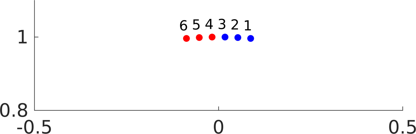
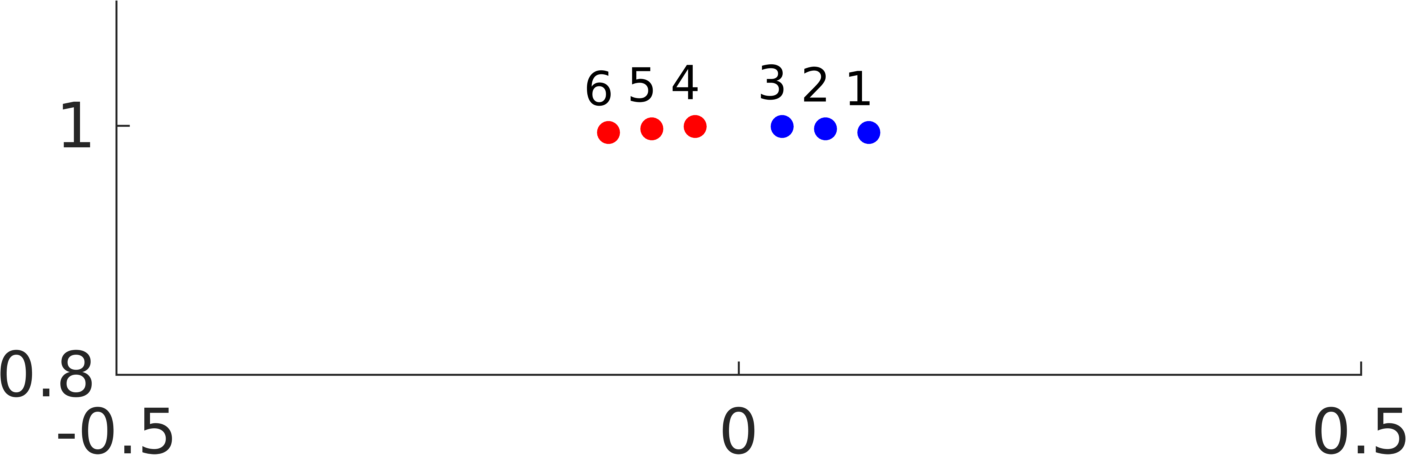
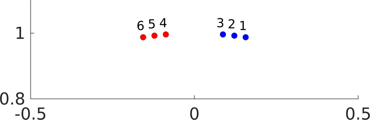
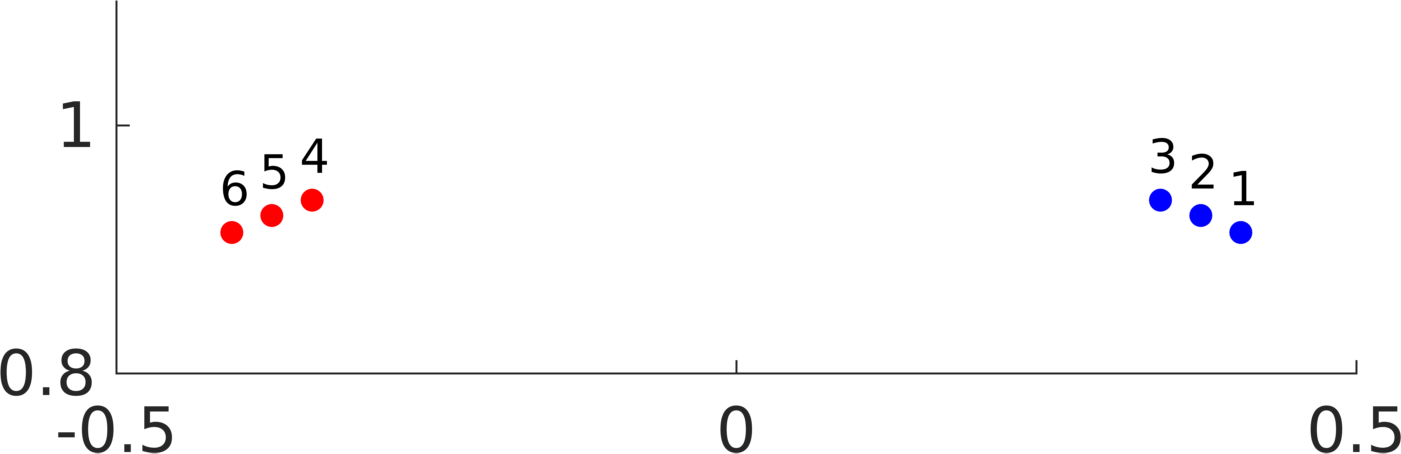
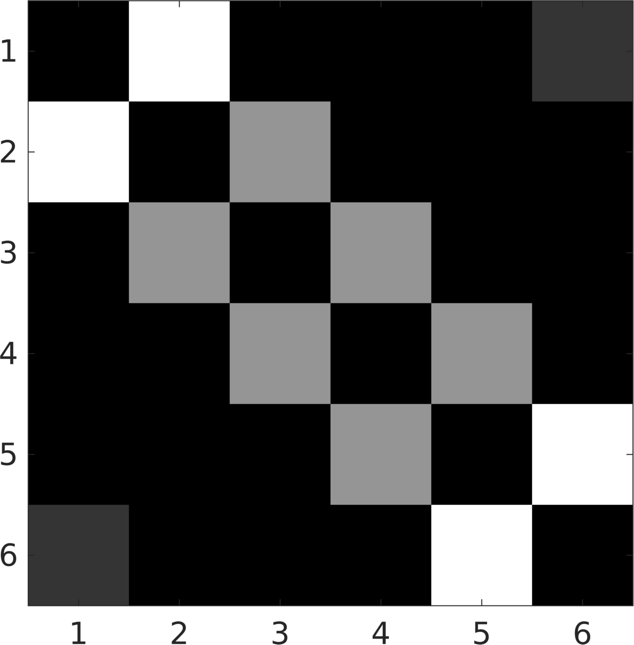
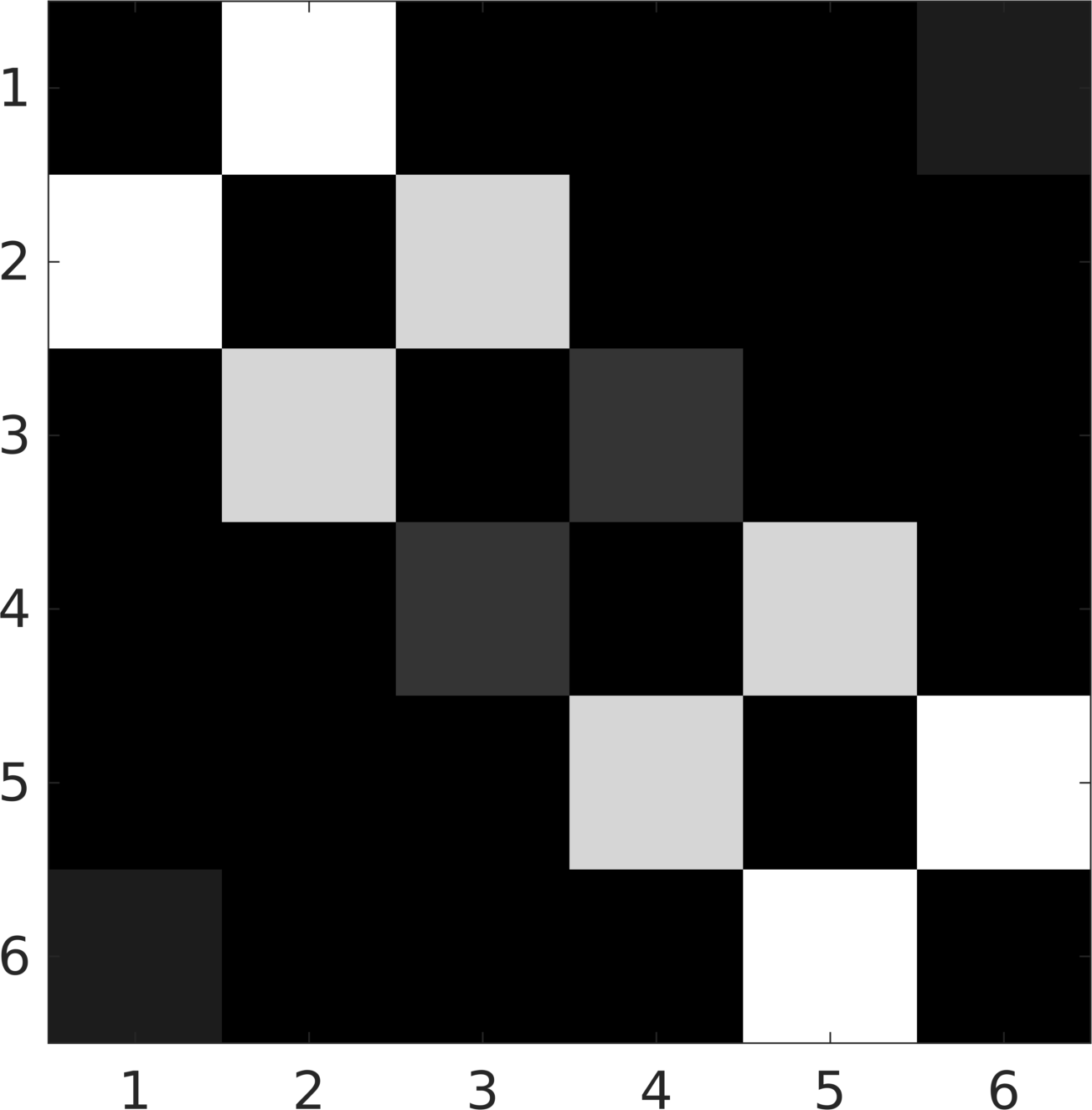
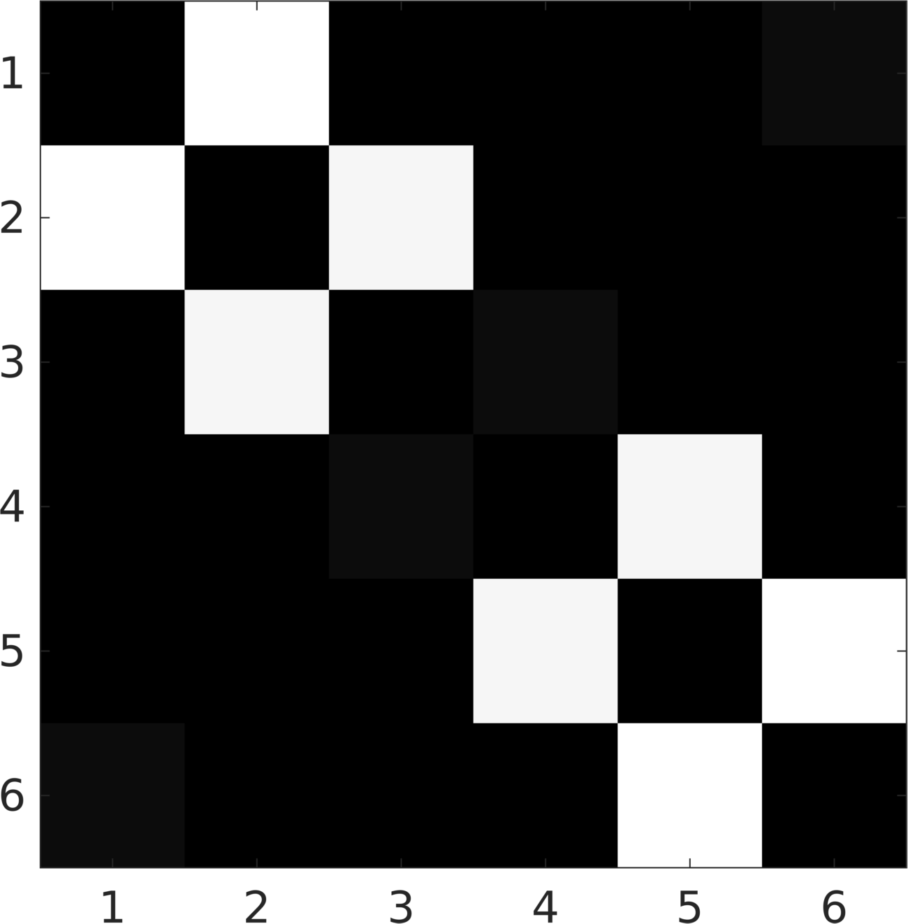
Figure 1: Upper row: two sets of points (red and blue) separated by angles of $2^{\circ}$, $4^{\circ}$, $10^{\circ}$ and $20^{\circ}$ from left to right. Lower row: corresponding connectivity matrices $|C|+|C^{\top}|$ resulting from solving Eq. (2) with $\lambda=0.01$. The columns/rows correspond with the numbering of the points above.
The larger the angle between the two sets of points, the lower the connectivity between the two clusters as the magnitude of the entries on the anti-diagonal becomes smaller and smaller. For an angle of $20^{\circ}$, the two sets almost form two disconnected clusters.

Bold lower-case letters $\mathbf{x}$ indicate vectors, normal capital letters matrices, e.g. $X=[\mathbf{x}_{1}\;\cdots\;\mathbf{x}_{N}]$, or constants, e.g. $N$. By $\mathbf{x}(j)$, we mean the $j$th element of vector $\mathbf{x}$, and by $A(i,j)$ the $(i,j)$th entry of matrix $A$. Sparse subspace clustering rests upon the assumption that there are $L$ subspaces $\mathcal{S}^{(l)}\in I\!\!R^{m}$, $l=1,\ldots,L$ with $N_{l}$ points $X^{(l)}=[\mathbf{x}^{(l)}_{1},\ldots,\mathbf{x}^{(l)}_{N_{l}}]$ on it. Let $d^{(l)}$ denote the dimension of $\mathcal{S}^{(l)}$. Let $X=[X^{(1)}\,\ldots\,X^{(L)}]$ denote the matrix of all $N_{1}+\cdots+N_{L}=N$ data points. Assume without loss of generality that $X$ is ordered. The points $\mathbf{x}_{j}$ are supposed to have unit length $\|\mathbf{x}_{j}\|_{2}=1$.

Let $T^{(l)}$ indicate the set of indices of all the points $\mathbf{x}^{(l)}\in\mathcal{S}^{(l)}$. Let $S_{j}\subseteq T^{(l)}$ indicate the support set of point $\mathbf{x}_{j}$, $j=\{1,\ldots,N\}$. The cardinality of a set is denoted by $|\cdot|$. The $k$th point of the support set $S_{j}$ of $\mathbf{x}^{(l)}_{j}$ is denoted by $\mathbf{x}^{(l)}_{j,k}$. Let $\mathbf{y}$ be any of the points of $X$. The matrix $X_{-y}$ indicates the matrix $X$ without the column corresponding to $\mathbf{y}$.

By $\|\cdot\|_{\{0,1,2,F\}}$ we indicate the $l0$-pseudo-norm, or the $l1$-, $l2$-, or Frobenius-norm of the argument.

3 Sparse Subspace Clustering

Sparse subspace clustering (SSC) (?) is based on the fact that any point $\mathbf{x}_{j}\in\mathcal{S}^{(l)}$ can be expressed by a linear combination of $d^{(l)}$ other points in the same subspace. Since such linear combinations do not use points of other classes, they can be used to infer the unknown class labels.

The problem is to compute the least number of points $\mathbf{x}_{k}$, $k\neq j$ such that a linear combination of the $\mathbf{x}_{k}$ yields $\mathbf{x}_{j}$. Denote by $\mathbf{c}_{j}$ the vector of mixing coefficients with its $j$th entry being equal to zero such that $\mathbf{x}_{j}=X\mathbf{c}_{j}$ holds true. The task to estimate the vector $\mathbf{c}_{j}$ can be solved by minimizing

$$\min{\|\mathbf{c}_{j}\|_{0}}\quad s.t.\quad\|X\mathbf{c}_{j}-\mathbf{x}_{j}\|_{2}^{2}=0\;\;\mbox{and}\;\;c_{jj}=0.$$ (1)

Since optimizing the $l_{0}$-norm is difficult, it is often approximated by using the $l_{1}$-norm. Allowing for data points $\mathbf{x}_{j}$ contaminated by noise, it is possible to instead optimize

$$\min{\|\mathbf{c}_{j}\|_{1}}\quad s.t.\quad\|X\mathbf{c}_{j}-\mathbf{x}_{j}\|_{2}^{2}\leq\lambda\;\;\mbox{and}\;\;c_{jj}=0.$$ (2)

for a scalar $\lambda>0$.

Given the matrix $C=\begin{bmatrix}\mathbf{c}_{1}&\cdots&\mathbf{c}_{N}\end{bmatrix}$, class labels can be inferred by means of spectral clustering of the graph $G=(V,E)$ with $|V|=N$ vertices corresponding to the points $\mathbf{x}_{j}$ and edge weights $E_{ij}$ defined by the matrix $|C|+|C|^{\top}$. These steps are the basis of the so-called sparse subspace clustering (SSC) algorithm proposed in (?).

4 Subspace Connectivity in $I\!\!R^{2}$

Since only few edge weights are known, the authors of (?) raised the question whether connectivity between vertices of the same cluster is always guaranteed. In other words, is the subgraph consisting of the vertices of one particular cluster connected? Their answer was that connectivity is guaranteed – and thus a correct result of SSC – if the subspace dimension is $d=2$ or $d=3$, but an example was given for $d=4$ where connectivity is violated. Independently, the authors of (?) concluded that SSC clusters correctly as long as the points are well spread within each cluster.

In this work, we will analyze the connectivity if the data is not well spread across each subspace but forms more or less well isolated clusters in a particular subspace. As an example, consider Fig. 1. Here, the upper row shows plots of two sets of points (depicted in red and blue). From left to right, the angle between the two sets increases from $2^{\circ}$ to $4^{\circ}$ and $10^{\circ}$ until $20^{\circ}$. The bottom row of Fig. 1 shows the corresponding affinity matrices $|C|+|C^{\top}|$ resulting from optimizing Eq. (2) with $\lambda=0.01$. The columns and rows correspond to the numbering of the points in the upper row of Fig. 1. It can be seen that the $(3,4)$ and $(4,3)$ entries have the same magnitudes as the $(2,3)$, $(3,2)$ and $(4,5)$, $(5,4)$ entries for an angle of $2^{\circ}$. However, at an angle of $20^{\circ}$, the entries on the anti-diagonal have almost negligible magnitude as compared to the other entries on the diagonal. Therefore, the resulting graph consists of two almost disconnected clusters.

Apparently, the question raised in (?), namely whether there is connectivity, i.e. are there non-zero entries in the affinity matrix, is not sufficient. The affinities shown on the anti-diagonal of the rightmost affinity are $>0$ yet their magnitude is negligible as compared to the other entries.

This example shows that spurious clusters can emerge if sparse coefficients are used as affinities. The example is equivalent to points on an affine line ($d=2$) normalized to unit length. It therefore readily generalizes to higher-dimensional structures in $I\!\!R^{m}$, $m>2$. The remainder of this paper focuses on the question how gaps between data on the same subspace influence the solutions $\mathbf{c}_{j}$ of Eq. (2) and thus the relative connectivity. The relative connectivities then determine if the corresponding vertices of the graph form more or less disconnected clusters.

5 The Bias of $l_{1}$-Norm Estimators

The analysis in this section solely concentrates on points on a single subspace $\mathcal{S}^{(l)}$. For the sake of simplicity, the superscript $(l)$ is omitted in the following.

Let the angle between two points $\mathbf{x}_{j_{1}}$ and $\mathbf{x}_{j_{2}}$, $j_{1}\neq j_{2}$ be defined by the inverse cosine of the scalar product of two unit length vectors, $\angle(\mathbf{x}_{j_{1}},\mathbf{x}_{j_{2}})=\mbox{acos}(\mathbf{x}_{j_{1}}^{\top}\cdot\mathbf{x}_{j_{2}})$. Assume without loss of generality that the points $\mathbf{x}_{j,k}$ are ordered such that $\angle(\mathbf{x}_{j},\mathbf{x}_{j,1})\geq\cdots\geq\angle(\mathbf{x}_{j},\mathbf{x}_{j,K})$.

Noiseless $l_{1}$-Norm: $\lambda=0$

Given a point $\mathbf{y}$, a matrix $X_{-y}$ and the $K$ points $\mathbf{x}_{y,k}$, $k=1,\ldots,K$ of a support set $S_{y}$ of $\mathbf{y}$, and let $\mathbf{c}_{y}$ be a solution to $\|X_{-y}\mathbf{c}_{y}-y\|_{2}^{2}\leq\lambda$ so that all entries but those corresponding to the points $\mathbf{x}_{y,k}$ in $X_{-y}$ are zero. The question then is how does $\|\mathbf{c}_{y}\|_{1}$ change if a different support set $S_{y}^{\prime}\subseteq T_{y}$ is selected.

The geometry of this case is shown in the left plot of Fig. 2. The intersection of the red dash-dotted line with the line through the point $\mathbf{x}_{y,1}$ indicates the point $c_{y}(1)\mathbf{x}_{y,1}$. The point $\mathbf{s}$ indicates the intersection of this line with the subspace $\mbox{span}(Q)$ spanned by the remaining points $Q=\begin{bmatrix}\mathbf{x}_{y,2}&\cdots&\end{bmatrix}$. It can be seen that $\|\mathbf{s}\|_{1}$ grows as the angle $\theta$ between $\mbox{span}(Q)$ and $\mbox{span}(\mathbf{x}-\mathbf{y})$ decreases. This intuition motivates the following proposition:

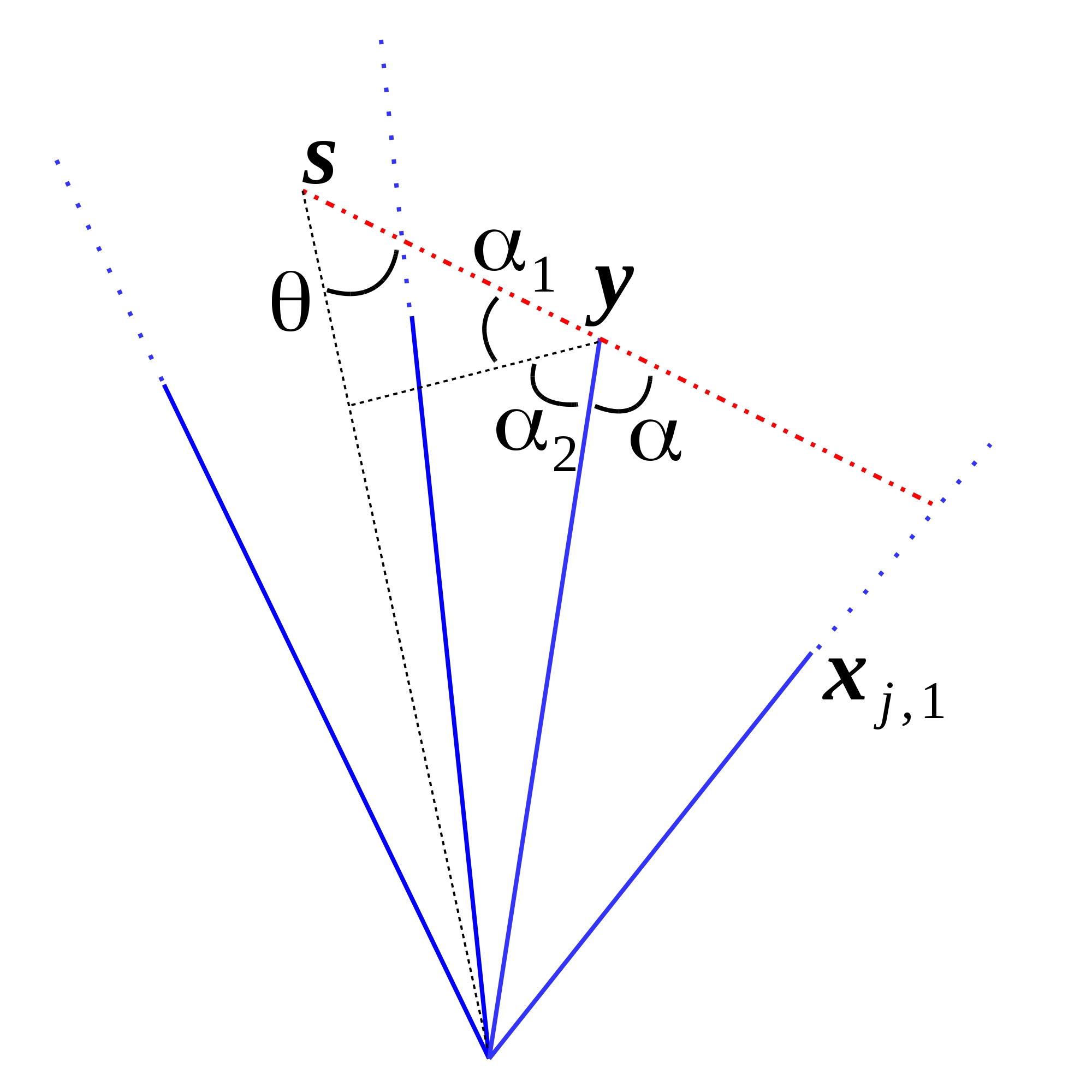
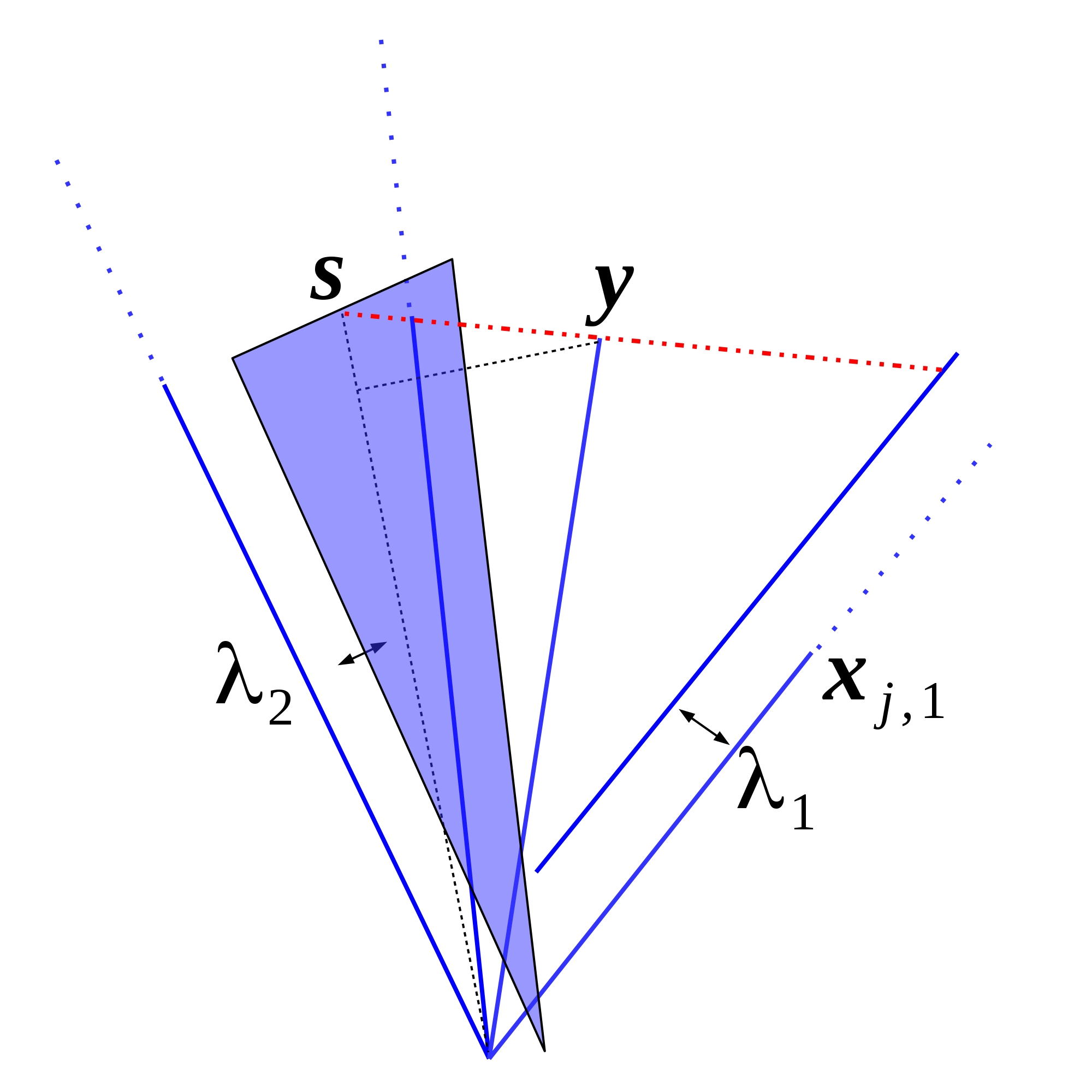
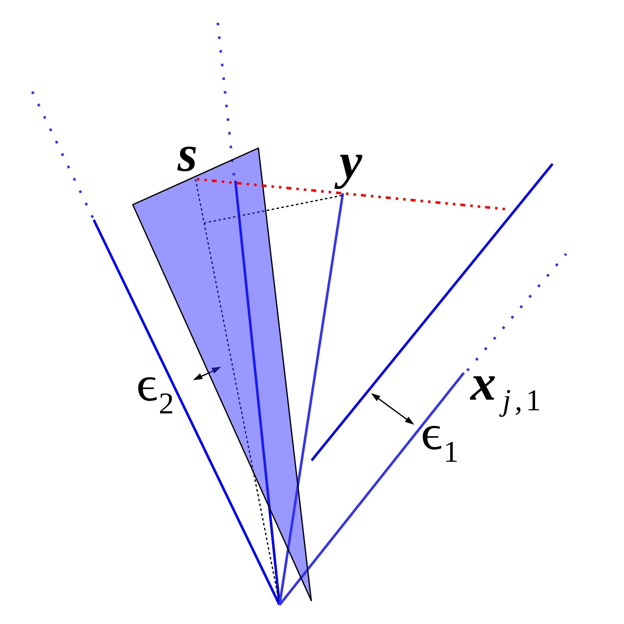
Figure 2: Geometry of different $l_{1}$-norm estimators. Left: noiseless case (Eq. (2) with $\lambda=0$); middle: noisy $l_{1}$-norm (Eq. (2) with $\lambda>0$); right: lasso.

Proposition 1.

The $l_{1}$-norm of $\mathbf{c}_{y}$ increases with the angle $\angle\left(\mathbf{y},\mathbf{x}_{y,1}\right)$ between $\mathbf{y}$ and $\mathbf{x}_{y,1}$

$$\|\mathbf{c}_{j}\|_{1}\geq\cot\left(f\left(\angle\left(\mathbf{y},\mathbf{x}_{y,1}\right)\right)+\rho-\frac{\pi}{2}\right)\cdot\eta.$$ (3)

Proof.

Let $\mathbf{v}_{1}=(c_{j,1}\mathbf{x}_{y,1}-\mathbf{y})/\|c_{j,1}\mathbf{x}_{y,1}-\mathbf{y}\|_{2}$, $\mathbf{v}_{2}=(P_{Q}\mathbf{y}-\mathbf{y})/\|P_{Q}\mathbf{y}-\mathbf{y}\|_{2}$ where $P_{Q}$ is the orthogonal projector onto $\mbox{span}(Q)$, and $f\left(\angle\left(\mathbf{y},\mathbf{x}_{y,1}\right)\right)=\cos^{-1}\mathbf{v}_{1}$. Let $\alpha=\cos^{-1}\mathbf{v}_{1}^{\top}\mathbf{y}$ be the angle between the line connecting $\mathbf{y}$ and $c_{j,1}\mathbf{x}_{y,1}$. Assuming that $|T_{y}|>|S_{y}|$, the support set $\mathbf{x}_{y,2},\ldots$ is selected such that $\mbox{span}(Q)\perp\mbox{span}(\begin{bmatrix}\mathbf{y}&\mathbf{x}_{y,1}\end{bmatrix})$ in order to minimize $\|\mathbf{x}\|_{2}$. Then, we can define the angles $\alpha_{1}=\cos^{-1}-\mathbf{y}^{\top}\mathbf{v}_{2}$, $\alpha_{2}=\pi-\alpha-\alpha_{1}$, and $\theta=\alpha+\alpha_{1}-\pi/2$ which motivates

$$\|\mathbf{x}-P_{Q}\mathbf{y}\|_{2}=\mbox{cotan}\,\theta\cdot\|(I-P_{Q})\mathbf{y}\|_{2}.$$ (4)

If we now define $\boldsymbol{\nu}=(I-P_{Q})\mathbf{y}$, $\eta=\|\boldsymbol{\nu}\|_{2}$, and $\rho=\cos^{-1}(\mathbf{y}^{\top}\boldsymbol{\nu})/\eta$ we arrive at the claim since $\|\mathbf{y}\|_{1}\geq\|\mathbf{y}\|_{2}$.∎

Given $\mathbf{y}$, and $d$ points $\mathbf{x}_{y,1},\ldots,\mathbf{x}_{y,d}$ of a support set $S_{y}$ and the corresponding sparse solution $\mathbf{c}_{S}$ to $\|X_{-y}\mathbf{c}_{S}-\mathbf{y}\|_{2}=0$. Let $\mathcal{H}(\mathbf{y},Q)$ be the plane through $\mathbf{y}$ with orthonormal basis $Q$. Assume that there is a point $\mathbf{x}_{n}\in X_{T_{y}\setminus S_{y}}$ with $\angle\left(\mathbf{y},\mathbf{x}_{n}\right)<\angle\left(\mathbf{y},\mathbf{x}_{y,1}\right)$ on the same side of $\mathcal{H}(\mathbf{y},Q)$ as $\mathbf{x}_{y,1}$. Let $S^{\prime}_{y}$ be the set of indices of the points $\mathbf{x}_{n},\mathbf{x}_{y,2},\ldots,\mathbf{x}_{y,d}$ and $\mathbf{c}_{s^{\prime}}$ be the solution to $\|X_{-y}\mathbf{c}_{S^{\prime}}-\mathbf{y}\|_{2}=0$.

Proposition 2.

The solution $\mathbf{c}_{s^{\prime}}$ of $\|X_{-y}\mathbf{c}_{S^{\prime}}-\mathbf{y}\|_{2}=0$ satisfies

$$\|\mathbf{c}_{S^{\prime}}\|_{1}<\|\mathbf{c}_{S}\|_{1}.$$ (5)

Proof.

The proof follows from Prop. 3. ∎

Corollary 1.

The $d$ points $\mathbf{x}_{y,1},\ldots,\mathbf{x}_{y,d}\in X_{T_{y}}$ closest to $\mathbf{y}$ minimize $\|\mathbf{c}\|_{1}$ such that $\|X_{-y}\mathbf{c}-\mathbf{y}\|_{2}=0$.

The implication is as follows: The usual assumption is that the data uniformly distributed. In the context of sparse subspace clustering, this implies that data on the same subspace need be uniformly distributed (cf. (?)). If this condition is violated, for instance because points fall into two well separated clusters, the support of the points of one cluster will not include points of the other.

This does not change the results in (?) since the central Theorem 2.5 there rests upon the assumption that points on the same subspace are more or less evenly distributed. The idea in this work considers a particular violation of this assumption.

Robust $l_{1}$-Norm: $\lambda>0$

Define $\lambda_{1}$ and $\lambda_{2}$ such that $\lambda_{1}+\lambda_{2}=\lambda$. The idea here is to define an auxiliary line parallel to $\mbox{span}\begin{bmatrix}\mathbf{x}_{y,1}\end{bmatrix}$ with distance $\lambda_{1}$ into direction of $\mathbf{y}$, and an auxiliary subspace parallel to $\mbox{span}\begin{bmatrix}\mathbf{x}_{y,2}&\cdots&\end{bmatrix}$ with distance $\lambda_{2}$ also into direction of $\mathbf{y}$. The geometry of this configuration is shown in the middle of Fig. 2.

Proposition 3.

The $l_{1}$-norm of $\mathbf{c}$ increases with the angle $\angle\left(\mathbf{y},g\left(\mathbf{x}_{y,1},\lambda_{1}\right)\right)$ between $\mathbf{y}$ and $g\left(\mathbf{x}_{y,1},\lambda_{1}\right)$

$$\|\mathbf{c}\|_{1}\geq h_{2}\left(\eta,\lambda_{2}\right)\cdot\\ \cot\left(f\left(\angle\left(\mathbf{y},g\left(\mathbf{x}_{y,1},\lambda_{1}\right)\right)\right)+h_{1}\left(\rho,\lambda_{2}\right)-\frac{\pi}{2}\right).$$ (6)

Proof.

The idea for the robust $l_{1}$-norm estimator is to create auxiliary variables $\lambda_{1}$ and $\lambda_{2}$ so that $\lambda=\lambda_{1}+\lambda_{2}$. These two are used to define two affine spaces parallel to $\mbox{span}(\mathbf{x}_{y,1})$ and $\mbox{span}(Q)$ with distances $\lambda_{1}$ and $\lambda_{2}$ such that the distances to $\mathbf{y}$ are reduced by $\lambda_{1}$ and $\lambda_{2}$. The function $g$ constructs the affine space parallel to $\mbox{span}(\mathbf{x}_{y,1})$. The functions $h_{1}$ and $h_{2}$ modify the projection of $\mathbf{y}$ not onto $\mbox{span}(Q)$ but its parallel affine space, and correct $\rho$, respectively. ∎

Lasso

The configuration for the lasso estimator

$$\min\;\|\mathbf{c}\|_{1}+\lambda\cdot\|X_{-y}\mathbf{c}-\mathbf{y}\|_{2}$$ (7)

is very similar to the one shown for the robust $l_{1}$-norm and is shown in the right plot of Fig. 2. We can now define a variable $\epsilon=\epsilon_{1}+\epsilon_{2}$ that it absorbs the $l_{2}$-error. Here $\epsilon_{1}$ indicates the distance of an auxiliary line parallel to $\mbox{span}\begin{bmatrix}\mathbf{y}\end{bmatrix}$ with distance $\epsilon_{1}$ and an auxiliary subspace parallel to $\mbox{span}\begin{bmatrix}\mathbf{x}_{y,2}&\cdots&\end{bmatrix}$ with distance $\epsilon_{2}$. The difference to the robust $l_{1}$-norm is that $\epsilon$ is now variable.

Due to the close similarity between the two estimators, Proposition 6 can easily be adapted to the lasso estimator:

Proposition 4.

The $l_{1}$-norm of $\mathbf{c}$ is increases with the angle $\angle\left(\mathbf{y},g\left(\mathbf{x}_{y,1},\lambda_{1}\right)\right)$ between $\mathbf{y}$ and $g\left(\mathbf{x}_{y,1},\lambda_{1}\right)$

$$\|\mathbf{c}\|_{1}\geq h_{2}\left(\eta,\epsilon_{2}\right)\cdot\\ \cot\left(f\left(\angle\left(\mathbf{y},g\left(\mathbf{x}_{y,1},\epsilon_{1}\right)\right)\right)+h_{1}\left(\rho,\epsilon_{2}\right)-\frac{\pi}{2}\right).$$ (8)

Proof.

The proof of Proposition 8 is identical as the one of Prop. 6 except that the admissible error $\epsilon=\epsilon_{1}+\epsilon_{2}$ is now variable. ∎

6 Selective Pursuit

Selective Dantzig Selector

Inspired by the Dantzig selector (?; ?), $X^{\star}=X^{\top}$, we notice that the product $X^{\star}X$ measures correlations to the subspace if we define a modified Dantzig selector

$$X^{\star}=X_{S_{y}}^{\top}.$$ (9)

The matrix $X_{S_{y}}$ consists of those columns of $X$ that are the support of $\mathbf{y}$. Since points on the same subspace have smaller distances to it than points from different subspaces, we can expect that the products $X^{\star}\mathbf{x}_{j}$, $j=1,\ldots,N\;\setminus\,\{\mathcal{I}(\mathbf{y}),\,\mbox{supp}(\mathbf{y})\}$ to be large if $j\in T_{y}$.

The idea proposed here is as follows: The support set $S_{y}$ of $\mathbf{y}$ usually consists of points from the set of neighbors of $\mathbf{y}$. Rather than stopping at this point, it is possible to select additional points, if their coherences with $\mbox{span}(X_{S_{y}})$ is are large.

Let $S^{e}_{y}$ be the extended support set of $\mathbf{y}$ which consists of the original support set, and the additionally selected points. If the modified Dantzig selector is now taken to be $X^{\star}=X_{S^{e}_{y}}^{\top}$, the selection process becomes more and more influenced by noise. Because noise causes spurious singular values in $X^{\star}$, we reduce their effect by scaling with

$$\rho=\mbox{trace}(X^{\star})^{\top}X^{\star}.$$ (10)

Since the trace of the square of a matrix equals the sum of its singular values, this reduces the effect of the spurious singular values. Finally, new extended support vectors are chosen if for a threshold $\delta$

$$\operatorname*{arg\,max}\limits_{j}\frac{\|X^{\star}\mathbf{x}_{j}\|_{2}^{2}}{\rho}>\delta,\quad j\in\{1,\ldots N\}\setminus\{\mathcal{I}(\mathbf{y}),\,S^{e}_{y}\}.$$ (11)

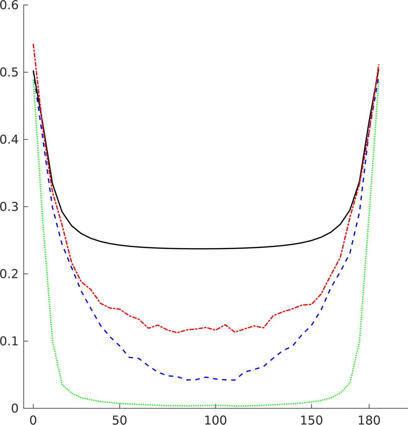
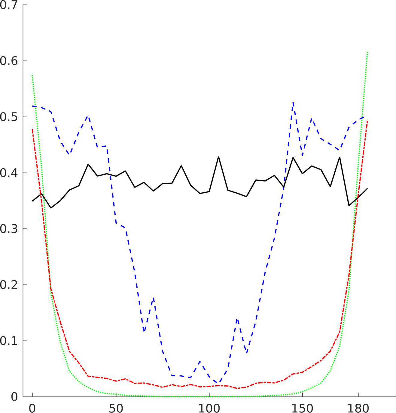
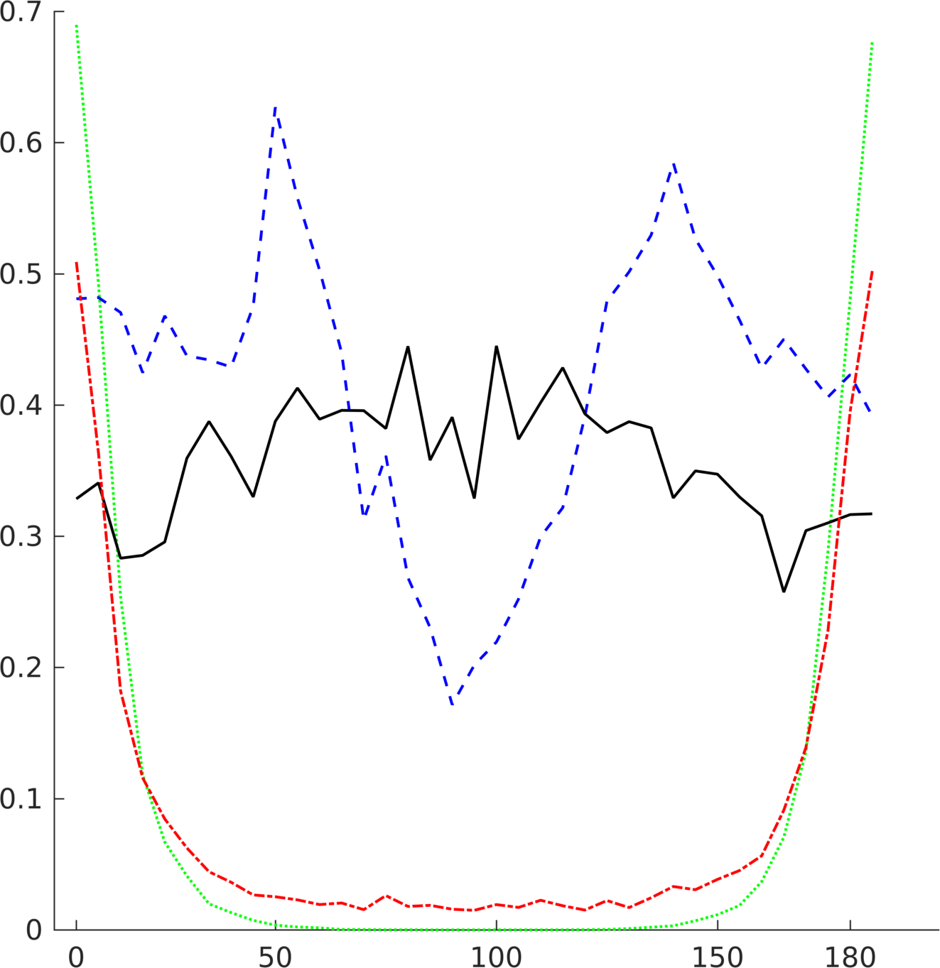
Figure 3: Relative connectivities between the two clusters. The $x$-axes correspond to angles between the clusters (cf. the explanation in Sec. 7), the $y$-axes to the relative connectivity $\xi$ defined by Eq. (15). Left: no noise; middle: noise with $\sigma=1\%$; right: noise with $\sigma=2\%$. The dotted green line corresponds to the lasso-method, the dash-dotted red line to the variational l0-norm optimization (?), the dashed blue line to the proposed Selective Dantzig Selector, and the solid black line to the proposed Subspace Selector.

Subspace Selector

To further reduce the effect of spurious singular values, it is possible to fit an $d^{(l)}\approx\mbox{length}(S_{y})$ dimensional orthonormal basis $B$ to $X^{\star}$

$$B=\operatorname*{arg\,max}\sum\|BX^{\star}_{j}\|_{2}^{2},\quad j=1,\ldots,\mbox{length}(S^{e}_{y}).$$ (12)

We can now choose additional points based on the Euclidean distance to the subspace $\mbox{span}(B)$ by

$$\operatorname*{arg\,max}\limits_{j}\|P_{B}\mathbf{x}_{j}\|_{2}^{2}>\delta,\quad j\in\{1,\ldots N\}\setminus\{\mathcal{I}(\mathbf{y}),\,S^{e}_{y}\}.$$ (13)

for a threshold $\delta$. Here, $P_{B}$ is the orthogonal projector onto $\mbox{span}(B)$.

7 Experiments

To experimentally demonstrate the effect of disconnectivity between clusters of points on the same subspace, we created two normally distributed point clouds on the unit sphere in $I\!\!R^{3}$ with identical mean and standard deviation. Each clusters consists of $20$ points. One was then rotated in steps of $5^{\circ}$ from $0^{\circ}$ to $180^{\circ}$. Afterwards, both point sets were multiplied by the same orthonormal $20\times 3$ basis matrix. Each point was then normalized to length $1$.

For each angle between the clusters, normally distributed noise was added to the data. We used standard deviations of $\sigma=\{0,0.02,0.03\}$ which amounts to $0\%$, $2\%$, and $3\%$ noise. For each combination and noise magnitude, $10$ trials were performed, i.e. the data was perturbed $10$ times with different random noise.

To measure the connectivity between the two point sets, we analyzed the affinity matrix $A=|C|+|C^{\top}|$

$$A=\begin{bmatrix}A_{11}&A_{12}\\ A_{21}&A_{22}\end{bmatrix}.$$ (14)

The coefficients in the $A_{11}$ and $A_{22}$ blocks indicate the connectivity within each cluster whereas the coefficients in $A_{21}=A_{12}^{\top}$ indicate the connectivity between the different clusters.

We can therefore measure the connectivity $\xi$ between the clusters by

$$\xi=\frac{1}{N}\sum\limits_{i=1}^{N}\frac{\sum\limits_{j=1}^{N_{2}}A_{12}(i,j)}{\sum\limits_{j=1}^{N}A(i,j)}$$ (15)

The two algorithms proposed in Sec. 6 are compared against a lasso-estimator

$$\|\mathbf{c}_{c}\|_{1}+\lambda\|Y_{-j}\mathbf{c}_{c}-\mathbf{y}\|_{2}$$ (16)

which is optimized using CVX (?). We used only Eq. (16) because the results of Eq. (2) are almost identical. Further, an algorithm to estimate the $l0$-norm using a variational approach (?) was included into the comparison. This is motivated by the idea that the $l0$-norm is not supposed to be effected by the bias that the $l1$-norm estimators have.

The results are shown in the plots in Fig. 3. The left plot corresponds to no noise, the middle one to a medium noise ($\sigma=1\%$), and the right plot to strong noise ($\sigma=2\%$). The $x$-axes correspond to angles between the clusters (cf. the explanation in Sec. 7), the $y$-axes to the relative connectivity $\xi$ defined by Eq. (15). The dotted green line indicates the lasso-method (16), the dash-dotted red line the l0-norm optimization, the dashed blue line the proposed Selective Dantzig Selector, and the solid black line the proposed Subspace Selector.

As can be seen, the two proposed algorithms do not suffer as much from the gap between the two clusters as the other algorithms. Very surprisingly, the $l0$-norm estimator is also strongly affected.

Average affinity matrices computed by three different methods are shown in Fig. 4. Apparently, for the lasso estimator the two clusters cause almost disconnected subgraphs at an angle of $45^{\circ}$ (left column in Fig. 4).

(a)

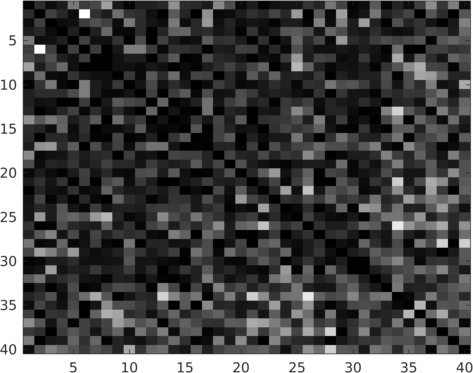
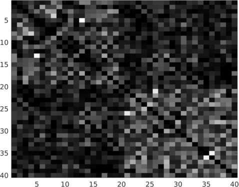
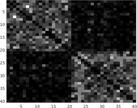
(b)

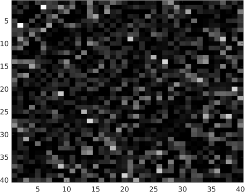
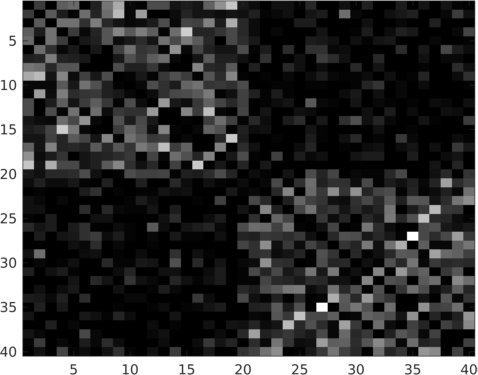
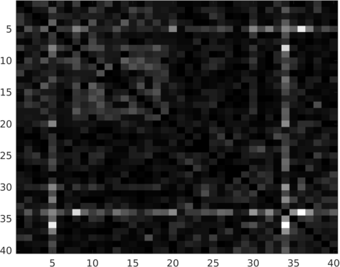
(c)

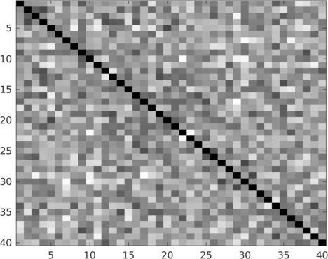
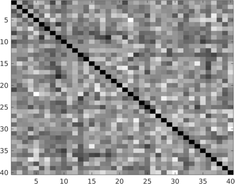
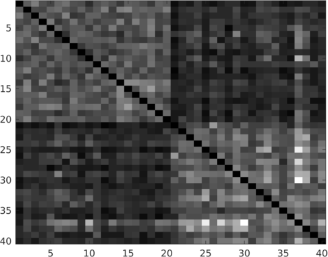
Figure 4: Average affinity matrices $A=|C|+|C^{\top}|$ of the ten trials with their entries normalized to $[0,1]$. The left column are the average affinities if the angle between the clusters is $0^{\circ}$. The middle column corresponds to angles of $10^{\circ}$, and the right one to $45^{\circ}$. (a) average affinities computed by the lasso estimator (16). (b) affinities compute by the variational estimator of the $l0$-norm (?). (c) affinities due to the proposed Selective Dantzig Selector.

8 Summary and Conclusions

The topic of this work is sparse subspace clustering. The principle idea behind this class of algorithms is to approximate each data point by a linear combination of as few other data points as possible. This problem is often approached by solving $l1$-norm problems. The sparse coefficients are used to define edge weights of a graph. Computing a minimum cut through this graphs reveals which points are located on the same subspace.

Since there are few edges per vertex, it could be possible that vertices of a graph form disconnected subgraph although the corresponding points lie on the same subspace. In a previous work, the possibility for this to happen was answered negatively if the subspace dimension is $2$ or $3$. Four $4$-dimensional subspaces, an example was given when disconnectivity occurs.

This work investigates the relaxed definition of not exact disconnectivity but relative disconnectivity. This means that all edge weights between two subgraphs are so low that the minimum cut either separates the two subgraphs, or – if the number of clusters is fixed – estimates a very erroneous result.

It is shown that this problem is caused by a gap between the points corresponding to the vertices of the subgraphs. In other words, if points on the same subspace fall into to separate clusters, then the two subgraphs necessarily have a so low connectivity that a successful clustering is no longer possible.

This problem does not invalidate the result published in (?), since the authors explicitly state that their Theorem 2.5 requires well distributed points. The idea in this work is to consider the case that this assumption is not given.

Two different algorithms are proposed which are not as susceptible to the shown effect. Surprisingly, even an estimator of the $l0$-norm suffers from biased distributions of points.

References

- [Candes and Tao 2007] Candes, E., and Tao, T. 2007. The dantzig selector: Statistical estimation when p is much larger than n. The Annals of Statistics 35(6):2392–2404.
- [CVX ] CVX: Software for Disciplined Convex Programming. www.cvx.com.
- [Elhamifar and Vidal 2013] Elhamifar, E., and Vidal, R. 2013. Sparse subspace clustering: Algorithm, theory, and applications. IEEE Transactions on Pattern Analysis and Machine Intelligence (TPAMI) 35(11):2765–2781.
- [Ho et al. 2003] Ho, J.; Yang, M.; Lim, J.; Lee, K.; and Kriegman, D. J. 2003. Clustering appearances of objects under varying illumination conditions. In Conference on Computer Vision and Pattern Recognition (CVPR), 11–18.
- [Hong et al. 2005] Hong, W.; Wright, J.; Huang, K.; and Ma, Y. 2005. A multi-scale hybrid linear model for lossy image representation. In International Conference on Computer Vision (ICCV), 764–771.
- [Kanatani 2001] Kanatani, K. 2001. Motion segmentation by subspace separation and model selection. In International Conference on Computer Vision (ICCV), 586–591.
- [Li and Vidal 2015] Li, C., and Vidal, R. 2015. Structured sparse subspace clustering: A unified optimization framework. In IEEE Conference on Computer Vision and Pattern Recognition (CVPR), 277–286. IEEE.
- [Liu, Lin, and Yu 2010] Liu, G.; Lin, Z.; and Yu, Y. 2010. Robust subspace segmentation by low-rank representation. In 27th International Conference on Machine Learning (ICML), 663–670.
- [Logsdon et al. 2012] Logsdon, B.; Carty, C.; Reiner, A.; Dai, J.; and Kooperberg, C. 2012. A novel variational bayes multiple locus z-statistic for genome-wide association studies with bayesian model averaging. Bioinformatics 28(13):1738–1744.
- [Nasihatkon and Hartley 2011] Nasihatkon, B., and Hartley, R. 2011. Graph connectivity in sparse subspace clustering. In IEEE Conference on Computer Vision and Pattern Recognition (CVPR), 2137–2144.
- [Patel, Nguyen, and Vidal 2013] Patel, V. M.; Nguyen, H. V.; and Vidal, R. 2013. Latent space sparse subspace clustering. In IEEE International Conference on Computer Vision (ICCV), 225–232.
- [Qu and Xu 2015] Qu, C., and Xu, H. 2015. Subspace clustering with irrelevant features via robust dantzig selector. In Advances in Neural Information Processing Systems (NIPS), 757–765.
- [Soltanolkotabi and Candes 2012] Soltanolkotabi, M., and Candes, E. 2012. A geometric analysis of subspace clustering with outliers. The Annals of Statistics 2195–2238.
- [Vidal, Ma, and Sastry 2005] Vidal, R.; Ma, Y.; and Sastry, S. 2005. Generalized principal component analysis (GPCA). IEEE Transations on Pattern Analysis and Machine Intelligence 27(12):1945–1959.
- [Zhang et al. 2012] Zhang, T.; Szlam, A.; Wang, Y.; and Lerman, G. 2012. Hybrid linear modeling via local best-fit flats. International Journal on Computer Vision 100(3):217–240.