The Spatial Distribution of Complex Organic Molecules in the L1544 Pre-stellar Core

Abstract

The detection of complex organic molecules (COMs) toward cold sources such as pre-stellar cores (with T$<$10 K), has challenged our understanding of the formation processes of COMs in the interstellar medium. Recent modelling on COM chemistry at low temperatures has provided new insight into these processes predicting that COM formation depends strongly on parameters such as visual extinction and the level of CO freeze out. We report deep observations of COMs toward two positions in the L1544 pre-stellar core: the dense, highly-extinguished continuum peak with A_V$\geq$30 mag within the inner 2700 au; and a low-density shell with average A_V$\sim$7.5-8 mag located at 4000 au from the core’s center and bright in CH₃OH. Our observations show that CH₃O, CH₃OCH₃ and CH₃CHO are more abundant (by factors $\sim$2-10) toward the low-density shell than toward the continuum peak. Other COMs such as CH₃OCHO, c-C₃H₂O, HCCCHO, CH₂CHCN and HCCNC show slight enhancements (by factors $\leq$3) but the associated uncertainties are large. This suggests that COMs are actively formed and already present in the low-density shells of pre-stellar cores. The modelling of the chemistry of O-bearing COMs in L1544 indicates that these species are enhanced in this shell because i) CO starts freezing out onto dust grains driving an active surface chemistry; ii) the visual extinction is sufficiently high to prevent the UV photo-dissociation of COMs by the external interstellar radiation field; and iii) the density is still moderate to prevent severe depletion of COMs onto grains.

1 Introduction

Complex Organic Molecules (COMs) are carbon-based species with $\geq$6 atoms in their molecular structure (Herbst & van Dishoeck, 2009). The most prolific regions in the detection of COMs in the interstellar medium (ISM) have been massive hot cores and Giant Molecular Clouds in the Galactic Center (SgrB2 (N) and (M); Hollis et al., 2000, 2006; Requena-Torres et al., 2008; Belloche et al., 2008, 2014) and low-mass hot corinos (IRAS16293-2422; Ceccarelli et al., 2000; Bottinelli et al., 2004; Jørgensen et al., 2012). Until recently, it was believed that COMs form on dust grains via hydrogenation (Charnley et al., 1995) or radical-radical reactions favoured by the heating from the central protostar (at T$\geq$30 K; see Garrod et al., 2008). However, the detection of COMs such as propylene (CH₂CHCH₃), acetaldehyde (CH₃CHO), dimethyl ether (CH₃OCH₃) or methyl formate (CH₃OCHO) in dark cloud cores and pre-stellar cores with T$\leq$10 K (B1-b, TMC-1, L1689B or L1544) has recently challenged our understanding of COM formation (Marcelino et al., 2007; Öberg et al., 2010; Bacmann et al., 2012; Cernicharo et al., 2012; Vastel et al., 2014; Loison et al., 2016).

Several mechanisms have been proposed to explain the presence of COMs in cold cores: gas-phase formation, non-canonical chemical explosions, cosmic-ray induced radical diffusion, impulsive spot heating of grains, or radical-radical recombination after H-atom addition/abstraction reactions on grain surfaces (Vasyunin & Herbst, 2013; Rawlings et al., 2013; Balucani et al., 2015; Reboussin et al., 2014; Ivlev et al., 2015; Chuang et al., 2016). However, information about the spatial distribution of COMs in cold cores is lacking (as well as of their radial abundance profile probing different density and extinction regimes), which prevents us from testing these COM formation scenarios.

The detection of a low-density, CH₃OH-rich shell around the continuum peak of the L1544 pre-stellar core (Bizzocchi et al., 2014) offers a unique opportunity to test COM formation scenarios in cold sources. Species such as C₃O, ketene (H₂CCO), formic acid (HCOOH) and acetaldehyde may be spatially co-located to CH₃OH in L1544 and may form at this low-density shell (Vastel et al., 2014). We report high-sensitivity observations of COMs toward two positions in the L1544 pre-stellar core: the continuum peak and a position within the low-density, CH₃OH-rich shell reported by Bizzocchi et al. (2014, hereafter the CH₃OH peak). Our results suggest that COMs are actively formed in the low-density shells of pre-stellar cores.

2 Observations

High-sensitivity single-pointing 3 mm observations were carried out toward two positions in the L1544 core during 10-16 December 2014 and 15-16 June 2016 with the Instituto de Radioastronomía Milimétrica (IRAM) 30 m telescope. We pointed our observations toward the core’s dust continuum peak, $\alpha$(J2000)=5^h04^m17.21^s, $\delta$(J2000)=25^∘10^′42.8$"$, and toward the CH₃OH peak, $\alpha$(J2000)=5^h04^m18^s and $\delta$(J2000)=25^∘11^′10$"$ (Bizzocchi et al., 2014). This position is $\sim$30$"$ away from the core’s center ($\sim$0.02 pc or 4000 au at 140 pc; Elias, 1978).

The observations were done in wobbler-switched mode with an angular throw of $\pm$120$"$. The dual sideband (2SB) EMIR E090 receivers were tuned at 84.37 GHz and 94.82 GHz with rejections $\geq$10 dB. We used three slightly different central frequencies (84.36, 84.37, 84.38 GHz and 94.80, 94.82, 94.84 GHz) to avoid the appearance of weak spurious features in the spectra. The FTS spectrometer allowed us to observe the inner part of each 4 GHz sub-bands covering 7.2 GHz in total, and it provided a spectral resolution of 50 kHz (0.15-0.18 km s^-1 at 3 mm). The observed frequency ranges were 83.4-85.2, 86.7-88.5, 99.1-100.9, 102.4-104.2 GHz and 78.2-80.0, 81.4-83.2, 93.9-95.7, 97.1-98.9 GHz. Typical system temperatures were 70-120 K. The beam size was $\sim$28-31$"$ between 79-87 GHz, and $\sim$24-26$"$ between 94-103 GHz. Intensities were calibrated in units of antenna temperature, T${}_{\rm A}^{*}$, and converted into main beam temperature, T_mb, by using beam efficiencies of 0.81 at 79-100 GHz, and 0.78 at 103 GHz. The RMS noise level was 1.6-2.8 mK for the core’s center position, and 2.2-3.7 mK for the CH₃OH peak.

3 Results

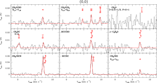
Figure 1: Sample of COM lines detected toward L1544’s dust continuum peak. Red lines show the Gaussian line fits derived for the COM transitions (see Table 1). The CH₃O spectrum has been extracted from the ASAI data (Vastel et al., 2014).

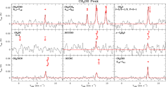
Figure 2: As in Figure 1, but for the position of the CH₃OH peak.

Figures 1 and 2 show some of the COM transitions detected toward L1544, while Table 1 lists all observed transitions and their derived line parameters. For completeness, we also provide the information about the covered transitions of acetaldehyde (CH₃CHO) – species already reported by Vastel et al. (2014) – and the upper limits of formamide (NH₂CHO), methyl isocyanate (CH₃NCO) and glycine (NH₂CH₂COOH). For all COMs the spectroscopic data were extracted from the JPL catalog (Pickett et al., 1998), except for dimethyl ether (CH₃OCH₃) for which we used SLAIM, and cyclopropenone (c-C₃H₂O), methyl isocyanate and glycine, for which we used the CDMS catalog (Müller et al., 2005).

Our high-sensitivity spectra reveal the detection of large COMs such as methyl formate (CH₃OCHO) and dimethyl ether (CH₃OCH₃) that had remained elusive in previous campaigns (see upper limits in Vastel et al., 2014). Other species detected are propynal (HCCCHO), cyclopropenone (c-C₃H₂O), ethynyl isocyanide (HCCNC) and vinyl cyanide (CH₂CHCN; Figures 1 and 2). Methoxy (CH₃O), considered as a COM precursor or COM dissociation product, is also detected toward the CH₃OH peak. All these molecules are observed at the $\sim$10-20 mK intensity level (Table 1). In Figure 1, we also report the tentative detection of methyl isocyanide (CH₃NC) toward the continuum peak. Its K=0,1 lines are detected at the 2.5$\sigma$ and 3.2$\sigma$ level. We are confident about the correct identification of all transitions since their derived radial velocities match the $\rm v_{\rm LSR}$ of the source (7.2 km s^-1), and for most species at least two transitions are detected. In addition, we have looked for other lines that could be blended and have found none. Since the COM line profiles are narrow (linewidths $\sim$0.3-0.4 km s^-1; Table 1), it is unlikely that they appear blended with unknown species.

Table 1 shows that the line emission from O-bearing species is either brighter toward the CH₃OH peak (by factors of $\sim$2-3 for CH₃O, CH₃CHO, CH₃OCHO and CH₃OCH₃), or remains constant toward both positions (HCCCHO and c-C₃H₂O). The N-bearing COMs HCCNC, CH₃NC and CH₂CHCN, on the contrary, show an opposite behaviour with brighter emission seen toward the center of the core. As shown in Section 5, this behaviour translates into larger enhancements toward the CH₃OH peak for CH₃O, CH₃CHO and CH₃OCH₃ than for the rest of COM species. Formamide, methyl isocyanate and glycine are not detected toward any position in L1544 (Table 1).

4 Excitation analysis of COMs

For CH₃O, CH₃OCHO, CH₃OCH₃, CH₃CHO, CH₃NC and CH₂CHCN, we have detected several lines so that a multi-line excitation analysis can be performed. The excitation temperature, T_ex, and total column density, N_obs, of these molecules have been calculated using the MADCUBAIJ software (Martín et al., 2011; Rivilla et al., 2016), assuming extended emission and LTE conditions. Except for CH₃NC (which is tentatively detected; Section  3), the derived T_ex is $\sim$5-6 K toward the core’s center and $\sim$5-8 K toward the CH₃OH peak (Table 2). Errors in Table 2 correspond to 1$\sigma$ uncertainties. We note that in some cases we had to fix T_ex to make MADCUBAIJ converge and find a solution. Since c-C₃H₂O is not included in MADCUBAIJ, we used the Weeds software for this molecule (Maret et al., 2011) and assumed that its emission fills the beam.

For the COMs with only one transition detected (and also for the non-detections), we again used MADCUBAIJ and assumed extended emission and a T_ex range of 5-10 K for both positions. This T_ex range agrees well with the values of T_ex obtained from the COM multi-line excitation analysis (Table 2), and with the T_ex measured from CH₃OH by Bizzocchi et al. (2014). The estimated values of N_obs are reported in Table 2.

5 COM abundance profiles in L1544

By calculating the COM molecular abundances toward the two positions in L1544, we can provide constraints to the COM abundance profiles as a function of radius within the core. For the continuum peak, we need to calculate the H₂ column density, N(H₂), within a radius of 13$"$ or 1900 au (i.e. half the IRAM 30 m beam of our observations). The N(H₂) of the core for radii $\leq$2500 au ($\sim$18$"$ at 140 pc) is nearly flat with a radius dependence N(H₂)$\propto r^{-0.8}$ (Ward-Thompson et al., 1999). By using the peak N(H₂) obtained by Crapsi et al. (2005, 9.4$\times$10²² cm^-2) for a radius of 6.5$"$ ($\sim$910 au), we derive that N(H₂)=5.4$\times$10²² cm^-2 for a radius of 13$"$ (1900 au). This value is similar to that estimated by Bacmann et al. (2000) for the same radius (4.5$\times$10²² cm^-2; see their Table 2). The slight difference is due to the dust temperatures assumed in both calculations (12.5 K in Bacmann et al. 2000 vs. 10 K in Crapsi et al. 2005). Hereafter, we use N(H₂)=5.4$\times$10²² cm^-2 for the position of the continuum peak within a radius of 13$"$.

For the CH₃OH peak, we assume an H₂ column density of 1.5$\times$10²² cm^-2 as derived by Spezzano et al. (2016) from Herschel data. The latter N(H₂) corresponds to a visual extinction $A_{V}$$\sim$15-16 mag using the Bohlin et al. (1978) formula. We note, however, that the model of L1544 by Keto & Caselli (2010) and Keto et al. (2014) considers the extinction as a function of radius (within the core and not along the line-of-sight) and therefore the modelled $A_{V}$ at this position is about half that measured along the line-of-sight ($A_{V}$$\sim$7.5-8 mag; see also Section 7).

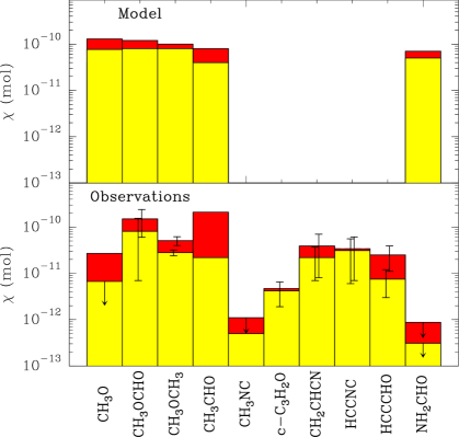
Figure 3: Comparison of the observed and modelled abundance of COMs toward the continuum peak (in yellow) and the CH₃OH peak (in red; see Section 5). The abundances shown for c-C₃H₂O, HCCNC and HCCCHO are average values. Error bars correspond to 1$\sigma$ uncertainties for CH₃OCHO, CH₃OCH₃ and CH₂CHCN, while they refer to the lower/upper abundance values estimated for c-C₃H₂O, HCCNC and HCCCHO (Table 2). Arrows indicate upper limit abundances.

From Table 2 and Figure 3 (lower panel), we find that CH₃O, CH₃OCH₃, CH₃CHO are enhanced respectively by factors $\geq$4-5, $\sim$2 and $\sim$10 in the CH₃OH peak with respect to L1544’s center (note that their associated 1$\sigma$ uncertainties are lower than these enhancements). The other O-bearing COMs CH₃OCHO, c-C₃H₂O and HCCCHO show average abundances slightly higher toward the CH₃OH peak than toward the core center (by factors $\leq$3), although they agree within the uncertainties. The same applies to the N-bearing COMs CH₂CHCN, CH₃NC and HCCNC, whose abundances lie within the uncertainties (Figure 3).

6 Upper limits to the abundance of pre-biotic COMs

The high-sensitivity spectra obtained toward L1544 allow us to provide stringent upper limits to the abundance of pre-biotic COMs such as glycine, NH₂CHO and CH₃NCO. As shown in Table 2, the derived upper limits to the column density of glycine are factors 40-120 lower than the best upper limits obtained toward the Galactic Center ($\leq$4$\times$10¹⁴ cm^-2; Jones et al., 2007). Our most stringent upper limit to the abundance of glycine in L1544 ($\leq$6$\times$10^-11; Table 2) is also a factor of 5 lower than that inferred for the outer envelope of IRAS16293-2422 ($\leq$3$\times$10^-10; Ceccarelli et al., 2000). Stacking analysis of the glycine lines with similar expected intensities in our frequency setup would reduce the rms noise level by a factor of $\sim$3 (10 lines are covered), which implies an upper limit of $\leq$2$\times$10^-11. This upper limit is close to the glycine abundance assumed by Jiménez-Serra et al. (2014) for the detectability of this molecule in pre-stellar cores ($\sim$3$\times$10^-11). The upper limits derived for NH₂CHO [$\leq$(2.4-8.7)$\times$10^-13] and CH₃NCO [$\leq$(0.2-4.2)$\times$10^-11; Table 2] are consistent with those measured in L1544 and B1-b by López-Sepulcre et al. (2015, $\leq$5$\times$10^-13) and Cernicharo et al. (2016, $\leq$2$\times$10^-12) respectively.

7 Chemical modelling of O-bearing COMs

In Section 5, we have reported abundance enhancements by factors $\sim$2-10 for CH₃O, CH₃OCH₃ and CH₃CHO as a function of distance in L1544. Other COMs such as CH₃OCHO may also be enhanced at larger radii although its derived abundances agree within the uncertainties (Section 5). In this Section, we model the chemistry of O-bearing COMs in L1544 by using the 1D physical structure derived by Keto & Caselli (2010) and Keto et al. (2014).

We use the chemical code of Vasyunin & Herbst (2013), which considers that COMs are formed via gas-phase ion-neutral and neutral-neutral reactions after the release of precursor molecules from dust grains via chemical reactive desorption. This code has been updated with a new multilayer treatment of ices, an advanced treatment of reactive desorption based on the experiments by Minissale et al. (2016), and new gas-phase reactions proposed by Shannon et al. (2013) and Balucani et al. (2015). The complete results from this modelling will be reported in Vasyunin et al., (in prep.).

The chemical evolution of COMs is followed over 3$\times$10⁶ years toward 129 points along the radius of the core to a distance $\sim$65500 au. For all these positions, the density, temperature and A_v are taken from Keto et al. (2014). The initial molecular abundances are calculated by simulating the chemistry of a translucent cloud with density n(H)=10² cm^-3 and T_gas=T_dust=20 K over 10⁶ years. The initial atomic abundances are the same as those of Vasyunin & Herbst (2013).

Our model shows that the abundances of COMs such as CH₃OCHO and CH₃OCH₃ change dramatically with time reaching maximum values at 10⁵-3$\times$10⁵ years. The gas-phase COM radial profiles show their peak abundances at $\sim$4000 au, which roughly coincides with the position of the CH₃OH peak (Bizzocchi et al., 2014). This is the location where CO starts freezing out onto dust grains in our model and it agrees well with the distance where CO depletion is observed in L1544 (see the drop in C¹⁷O reported by Caselli et al., 1999). The CO depletion enhances the production of COM precursors on grain surfaces via hydrogenation reactions while, at the same time, the visual extinction is sufficiently high ($A_{V}$$\sim$7.5-8 mag; Section 5) to prevent the UV photo-dissociation of the chemically desorbed COM precursors by the external interstellar radiation field. UV photo-desorption is not efficient at this position in the core and, therefore, the release of COMs into the gas phase is dominated by chemical reactive desorption. Toward the center of the core, the abundances of COMs drop to undetectable levels ($\leq$10^-14) as a result of the severe freeze out.

To compare the model results with our observations, one needs to sample all COM material along the line-of-sight toward the continuum and the CH₃OH peaks. The amount of COM material sampled in the direction of the CH₃OH peak will be larger than toward the continuum peak. While toward the core’s center COMs are found within a shell $R_{i-1}-R_{i}$ (with $R$ the radius from the center and $i$ the position in the grid with $i$=1 at the outermost shell), toward the CH₃OH peak COMs are sampled along a circle chord. For the core’s center the COM column density, $N(\rm{COM})$, is given by:

$$\begin{array}[]{l}N(\rm{COM})=2\times\sum_{\rm i=2}^{\rm n}\left[\frac{n(H)_{i}*\chi_{i}+n(H)_{i-1}*\chi_{i-1}}{2}\right]\times(R_{i-1}-R_{i})\end{array}$$ (1)

with $n$(H)_i the gas density at radial point $i$, $\chi_{i}$ the COM abundance, $(R_{i-1}-R_{i})$ the shell width, and $n$ the number of shells in the model ($n$=129). Toward the CH₃OH peak, $N(\rm{COM})$ is calculated as:

$$\begin{array}[]{l}N(\rm{COM})=2\times\sum_{\rm i=2}^{\rm n_{peak}}\left[\sqrt{R_{i-1}^{2}-R_{peak}^{2}}-\sqrt{R_{i}^{2}-R_{peak}^{2}}\right]{{}_{\times}}\\ \\ \ \ \ \ \ \ \ \ \ \ \ \ \ \ \ \ \ \ \ \ \ \ \ {{}_{\times}}\left[\frac{n(H)_{i}*\chi_{i}+n(H)_{i-1}*\chi_{i-1}}{2}\right]\end{array}$$ (2)

where R_peak is the radial distance of the CH₃OH peak (4000 au), n_peak is the radial point closest to this peak, and R_i and R_i-1 are the radii at positions $i$ and $i-1$. $N(\rm{COM})$ are averaged over the beam of the IRAM 30 m telescope ($\sim$26$"$), and the COM abundances are finally calculated by dividing the average $N(\rm{COM})$ by the $N(H_{2})$ obtained following the same method (4.0$\times$10²² cm^-2 for the continuum peak and 1.0$\times$10²² cm^-2 for the CH₃OH peak). Note that these values are similar to those used in Section 5. The best match with the observations is obtained at 10⁵ years.

Table 2 and Figure 3 (upper panel) report the predicted abundances of CH₃O, CH₃OCHO, CH₃OCH₃, CH₃CHO and NH₂CHO. The rest of O-bearing species (c-C₃H₂O, HCCCHO, CH₃NCO and glycine) are currently not included in the chemical network and their predictions are thus not reported. The modelled COM abundances reproduce the enhancements of CH₃OCH₃ and CH₃OCHO observed toward the CH₃OH peak within factors of 3 (Table 2 and Figure 3). For CH₃CHO, however, the model predicts a smaller enhancement than observed, although the modelled and observed CH₃CHO abundances agree within factors 2-3 for both positions. Large discrepancies are found for CH₃O and NH₂CHO (by factors $\sim$5-15 and $\sim$100-200, respectively; Table 2), which suggests that additional mechanisms are required to supress the production of these COMs in our model.

In summary, we report new detections of COMs in L1544. Species such as CH₃O, CH₃CHO and CH₃OCH₃ are enhanced by factors $\sim$2-10 toward the CH₃OH peak with respect to the core’s center. Other COMs such as CH₃OCHO may also be enhanced with increasing distance within the core (by factors $\leq$3), although their abundance uncertainties are large. Despite the discrepancies found between the observed COM abundances and those predicted in our model, O-bearing COMs are predicted to present an abundance peak at 4000 au, which agrees well with the position of the CH₃OH peak and with the radial distance at which CO depletion is observed. All this shows that high-sensitivity observations of COMs are strongly needed to put stringent constraints on chemical models and to step forward in our understanding of COM chemistry in the ISM.

Table 1: COM transitions covered in our observations and their derived line parameters

Species	Line	Frequency	$E_{\rm u}$	$g_{\rm u}$	$A_{\rm ul}$	(0$"$,0$"$)				CH3OH peak
						Area	VLSR	$\Delta v$	Tmb	Area	VLSR	$\Delta v$	Tmb
		(MHz)	(K)		(s-1)	(mK km s-1)	(km s-1)	(km s-1)	(mK)	(mK km s-1)	(km s-1)	(km s-1)	(mK)
CH3O	F=1$\rightarrow$0, $\Lambda$=-1	82455.98	4.0	3	6.5$\times$10-6	$\leq$3.7	$\ldots$	$\ldots$	$\leq$16.2	3.5(0.9)	7.06(0.03)	0.3(0.1)	10.8(2.4)
	F=2$\rightarrow$1, $\Lambda$=-1	82458.25	4.0	5	9.8$\times$10-6	$\leq$3.7	$\ldots$	$\ldots$	$\leq$15.9	9.2(1.1)	7.21(0.02)	0.40(0.05)	21.8(3.0)
	F=2$\rightarrow$1, $\Lambda$=+1	82471.82	4.0	5	9.8$\times$10-6	$\leq$3.9	$\ldots$	$\ldots$	$\leq$17.1	7.8(1.0)	7.22(0.02)	0.30(0.05)	24.3(2.9)
	F=1$\rightarrow$0, $\Lambda$=+1	82524.18	4.0	3	6.5$\times$10-6	$\leq$3.5	$\ldots$	$\ldots$	$\leq$15.0	2.6(0.9)	7.14(0.06)	0.27(0.08)	8.9(3.0)
CH3OCHO	91,9$\rightarrow$81,8 E	100078.608	25.0	38	1.4$\times$10-5	1.8(0.8)	7.23(0.10)	0.42(0.2)	4.1(2.0)	$\leq$1.7	$\ldots$	$\ldots$	$\leq$8.1
	91,9$\rightarrow$81,8 A	100080.542	25.0	38	1.4$\times$10-5	2.0(1.0)	7.22(0.19)	0.44(0.15)	4.4(1.7)	3.3(0.8)	7.16(0.03)	0.30(0.09)	10.4(2.6)
	83,5$\rightarrow$73,4 E	100294.604	27.4	34	1.3$\times$10-5	$\leq$1.3	$\ldots$	$\ldots$	$\leq$5.4	3.5(0.9)	7.20(0.04)	0.34(0.10)	9.9(2.5)
	83,5$\rightarrow$73,4 A	100308.179	27.4	34	1.3$\times$10-5	$\leq$1.7	$\ldots$	$\ldots$	$\leq$7.2	$\leq$1.4	$\ldots$	$\ldots$	$\leq$6.9
	81,7$\rightarrow$71,6 E	100482.241	22.8	34	1.4$\times$10-5	$\leq$4.1	$\ldots$	$\ldots$	$\leq$5.7	6.5(0.9)	7.17(0.02)	0.31(0.06)	19.6(2.7)
	81,7$\rightarrow$71,6 A	100490.682	22.8	34	1.4$\times$10-5	3.5(0.7)	7.21(0.04)	0.37(0.07)	8.9(2.2)	3.0(0.7)	7.16(0.03)	0.23(0.06)	12.3(2.6)
	90,9$\rightarrow$80,8 E	100681.545	24.9	38	1.5$\times$10-5	1.6(0.9)	7.16(0.11)	0.4(0.2)	4.1(2.8)	$\leq$1.6	$\ldots$	$\ldots$	$\leq$7.5
	90,9$\rightarrow$80,8 A	100683.368	24.9	38	1.5$\times$10-5	4.1(1.1)	7.12(0.07)	0.54(0.14)	7.2(2.7)	3.3(0.7)	7.11(0.03)	0.24(0.05)	13.1(2.6)
CH3OCH3	41,4$\rightarrow$30,3 EA	99324.357	10.2	36	2.2$\times$10-5	3.4(0.8)	7.11(0.05)	0.38(0.10)	8.4(2.4)	6.2(1.2)	7.11(0.03)	0.36 (0.08)	16.4(3.5)
	41,4$\rightarrow$30,3 AE	99324.359	10.2	54	3.3$\times$10-5	$\ldots$	$\ldots$	$\ldots$	$\ldots$	$\ldots$	$\ldots$	$\ldots$	$\ldots$
	41,4$\rightarrow$30,3 EE	99325.208	10.2	144	8.9$\times$10-5	4.0(0.8)	7.15(0.03)	0.32(0.07)	11.55(2.2)	9.6(1.2)	7.12(0.02)	0.39(0.06)	23.5(3.1)
	41,4$\rightarrow$30,3 AA	99326.058	10.2	90	5.5$\times$10-5	2.0(0.9)	7.22(0.09)	0.3(0.2)	5.4(2.5)	3.7(1.1)	7.12(0.05)	0.29(0.09)	12.0(3.7)
	62,5$\rightarrow$61,6 EA	100460.412	24.7	52	1.8$\times$10-5	$\leq$1.2	$\ldots$	$\ldots$	$\leq$5.8	$\leq$1.8	$\ldots$	$\ldots$	$\leq$7.8
	62,5$\rightarrow$61,6 AE	100460.437	24.7	78	2.6$\times$10-5	$\ldots$	$\ldots$	$\ldots$	$\ldots$	$\ldots$	$\ldots$	$\ldots$	$\ldots$
	62,5$\rightarrow$61,6 EE	100463.066	24.7	208	7.0$\times$10-5	$\leq$1.2	$\ldots$	$\ldots$	$\leq$5.7	1.4(0.8)	7.16(0.07)	0.26(0.16)	5.2(2.6)
	62,5$\rightarrow$61,6 AA	100465.708	24.7	130	4.4$\times$10-5	$\leq$1.3	$\ldots$	$\ldots$	$\leq$6.3	$\leq$1.8	$\ldots$	$\ldots$	$\leq$7.8
CH3CHO	21,2$\rightarrow$10,1 E	83584.260	5.0	10	2.2$\times$10-6	3.8(1.5)	7.12(0.04)	0.32(0.10)	10.9(2.6)	12.8(1.1)	7.18(0.01)	0.31(0.04)	39.0(3.1)
	21,2$\rightarrow$10,1 A	84219.764	5.0	10	2.4$\times$10-6	5.5(0.8)	7.21(0.02)	0.30(0.05)	17.4(2.5)	9.6(0.9)	7.12(0.01)	0.26(0.02)	34.4(3.0)
	21,1$\rightarrow$10,1 E	87109.504	5.2	10	1.3$\times$10-7	$\leq$1.4	$\ldots$	$\ldots$	$\leq$6.5	$\leq$1.7	$\ldots$	$\ldots$	$\leq$7.7
	22,0$\rightarrow$31,3 A	87146.655	11.8	10	2.9$\times$10-7	$\leq$1.3	$\ldots$	$\ldots$	$\leq$6.2	$\leq$1.5	$\ldots$	$\ldots$	$\leq$6.6
	22,0$\rightarrow$31,3 E	87204.278	11.9	10	1.1$\times$10-7	$\leq$1.6	$\ldots$	$\ldots$	$\leq$5.9	$\leq$1.7	$\ldots$	$\ldots$	$\leq$7.4
	63,4$\rightarrow$72,5 A	99141.294	24.4	10	7.1$\times$10-7	$\leq$1.4	$\ldots$	$\ldots$	$\leq$6.7	1.8(0.8)	6.95(0.03)	0.2(0.2)	8.1(3.0)
	63,4$\rightarrow$72,6 E	99490.149	24.3	10	6.1$\times$10-7	$\leq$1.4	$\ldots$	$\ldots$	$\leq$6.7	2.9(0.9)	7.33(0.07)	0.4(0.1)	6.3(2.3)
CH3NC	50$\rightarrow$40	100526.541	14.5	44	8.1$\times$10-5	4.0(1.0)	7.15(0.09)	0.66(0.18)	5.7(2.3)	$\leq$1.8	$\ldots$	$\ldots$	$\leq$7.5
	51$\rightarrow$41	100524.249	21.5	44	7.8$\times$10-5	2.6(0.7)	7.38(0.05)	0.35(0.11)	7.0(2.2)	$\leq$1.8	$\ldots$	$\ldots$	$\leq$7.5
	52$\rightarrow$42	100517.433	42.7	44	6.8$\times$10-5	$\leq$1.7	$\ldots$	$\ldots$	$\leq$6.9	$\leq$1.8	$\ldots$	$\ldots$	$\leq$7.5
c-C3H2O	61,6$\rightarrow$51,5	79483.520	14.6	39	5.1$\times$10-5	$\ldots$	$\ldots$	$\ldots$	$\ldots$	7.7(1.4)	7.09(0.03)	0.38(0.08)	18.8(3.0)
	71,6$\rightarrow$61,5	103069.925	21.1	45	1.1$\times$10-4	3.3(0.9)	7.18(0.06)	0.39(0.09)	8.0(2.8)	3.7(1.7)	7.1(0.1)	0.5(0.3)	7.6(3.4)
CH2CHCN	90,9$\rightarrow$80,8	84946.000	20.4	57	4.9$\times$10-5	24.78(1.0)	7.290(0.007)	0.397(0.019)	58.7(2.3)	6.6(1.1)	7.30(0.02)	0.29(0.06)	21.1(3.1)
	91,8$\rightarrow$81,7	87312.812	23.1	57	5.3$\times$10-5	13.2(0.9)	7.245(0.012)	0.35(0.03)	35.3(2.4)	5.1(1.1)	7.20(0.06)	0.46(0.09)	10.4(2.7)
	110,11$\rightarrow$100,10	103575.395	29.9	69	9.0$\times$10-5	7.8(0.8)	7.30(0.02)	0.42(0.05)	17.3(2.3)	$\leq$1.8	$\ldots$	$\ldots$	$\leq$8.7
HCCNC	10$\rightarrow$9	99354.250	26.2	63	4.6$\times$10-5	29.2(1.0)	7.227(0.005)	0.438(0.013)	62.7(1.6)	7.1(1.0)	7.17(0.03)	0.40(0.05)	16.5(2.2)
HCCCHO	90,9$\rightarrow$80,8	83775.842	20.1	19	1.8$\times$10-5	5.5(1.2)	7.08(0.06)	0.49(0.11)	10.6(2.8)	3.2(1.2)	7.04(0.06)	0.28(0.12)	10.8(3.5)
NH2CHO	40,4$\rightarrow$30,3	84542.400	10.2	11	4.1$\times$10-5	$\leq$1.8	$\ldots$	$\ldots$	$\leq$8.4	$\leq$2.3	$\ldots$	$\ldots$	$\leq$9.6
	41,3$\rightarrow$31,2	87848.915	13.5	11	4.3$\times$10-5	$\leq$1.3	$\ldots$	$\ldots$	$\leq$6.0	$\leq$1.8	$\ldots$	$\ldots$	$\leq$7.2
CH3NCO	101,10$\rightarrow$91,9	87506.605	29.0	21	3.0$\times$10-5	$\leq$1.1	$\ldots$	$\ldots$	$\leq$5.1	$\leq$1.2	$\ldots$	$\ldots$	$\leq$5.7
	12-1,12$\rightarrow$11-1,11	103023.61	39.4	25	4.9$\times$10-5	$\leq$1.3	$\ldots$	$\ldots$	$\leq$6.3	$\leq$1.6	$\ldots$	$\ldots$	$\leq$7.5
Glycine	65,2$\rightarrow$54,1	103294.648	15.2	39	1.6$\times$10-6	$\leq$1.7	$\ldots$	$\ldots$	$\leq$8.0	$\leq$2.1	$\ldots$	$\ldots$	$\leq$9.9
Conf I.	65,1$\rightarrow$54,2	103297.993	15.2	39	1.6$\times$10-6	$\leq$1.7	$\ldots$	$\ldots$	$\leq$8.0	$\leq$2.1	$\ldots$	$\ldots$	$\leq$9.9

Table 2: Excitation temperatures, column densities, and measured and modelled abundances of COMs in L1544

Species	(0$"$,0$"$)				CH3OH peak
	Tex (K)	Nobs (cm-2)	$\chi_{\rm obs}$	$\chi_{\rm mod}$	Tex (K)	Nobs (cm-2)	$\chi_{\rm obs}$	$\chi_{\rm mod}$
CH3O	5-10	$\leq$(2.8-3.6)$\times$1011	$\leq$(5.1-6.7)$\times$10-12	7.7$\times$10-11	8.0	4.0$\times$1011	2.7$\times$10-11	1.3$\times$10-10
CH3OCHO	5.1$\pm$2.3	(4.4$\pm$4.0)$\times$1012	(8.1$\pm$7.4)$\times$10-11	8.0$\times$10-11	7.9$\pm$3.6	(2.3$\pm$1.4)$\times$1012	(1.5$\pm$0.9)$\times$10-10	1.2$\times$10-10
CH3OCH3	5.7$\pm$3.1	(1.5$\pm$0.2)$\times$1012	(2.8$\pm$0.4)$\times$10-11	8.0$\times$10-11	7.6$\pm$3.7	(7.7$\pm$1.6)$\times$1011	(5.1$\pm$1.1)$\times$10-11	1.0$\times$10-10
CH3CHO	5.0	1.2$\times$1012	2.2$\times$10-11	4.0$\times$10-11	7.8	3.2$\times$1012	2.1$\times$10-10	8.0$\times$10-11
CH3NC	22.9	2.7$\times$1010	5.0$\times$10-13	$\ldots$	5-10	$\leq$(0.7-1.6)$\times$1010	$\leq$(0.5-1.1)$\times$10-12	$\ldots$
c-C3H2O	5-10	(1.0-3.5)$\times$1011	(1.9-6.5)$\times$10-12	$\ldots$	8.0	7.0$\times$1010	4.7$\times$10-12	$\ldots$
CH2CHCN	5.8$\pm$0.9	(1.2$\pm$0.8)$\times$1012	(2.2$\pm$1.5)$\times$10-11	$\ldots$	5.0$\pm$1.4	(5.8$\pm$4.7)$\times$1011	(3.9$\pm$3.1)$\times$10-11	$\ldots$
HCCNC	5-10	(0.3-3.0)$\times$1012	(0.6-5.6)$\times$10-11	$\ldots$	5-10	(1.0-9.1)$\times$1011	(0.7-6.1)$\times$10-11	$\ldots$
HCCCHO	5-10	(1.8-6.3)$\times$1011	(0.3-1.2)$\times$10-11	$\ldots$	5-10	(1.6-5.8)$\times$1011	(1.1-3.9)$\times$10-11	$\ldots$
NH2CHO	5-10	$\leq$(1.3-1.7)$\times$1010	$\leq$(2.4-3.1)$\times$10-13	5.0$\times$10-11	5-10	$\leq$(1.0-1.3)$\times$1010	$\leq$(6.7-8.7)$\times$10-13	7.0$\times$10-11
CH3NCO	5-10	$\leq$(0.8-6.3)$\times$1011	$\leq$(0.2-1.2)$\times$10-11	$\ldots$	5-10	$\leq$(0.9-6.3)$\times$1011	$\leq$(0.6-4.2)$\times$10-11	$\ldots$
Glycine	5-10	$\leq$(3.3-5.8)$\times$1012	$\leq$(0.6-1.1)$\times$10-10	$\ldots$	5-10	$\leq$(4.2-9.5)$\times$1012	$\leq$(2.8-6.3)$\times$10-10	$\ldots$

.

References

- Bacmann et al. (2012) Bacmann, A., Taquet, V., Faure, A., Kahane, C., & Ceccarelli, C. 2012, A&A, 541, L12
- Bacmann et al. (2000) Bacmann, A., André, P., Puget, J.-L., Abergel, A., Bontemps, S., & Ward-Thompson, D. 2000, A&A, 361, 555
- Balucani et al. (2015) Balucani, N., Ceccarelli, C., & Taquet, V. 2015, MNRAS, 449, L16
- Belloche et al. (2008) Belloche, A., Menten, K. M., Comito, C., et al. 2008, A&A, 482, 179
- Belloche et al. (2014) Belloche, A., Garrod, R. T., Müller, H. S. P., & Menten, K. M. 2014, Science, 345, 1584B
- Bizzocchi et al. (2014) Bizzocchi, L., Caselli, P., Spezzano, S., & Leonardo, E. 2014, A&A, 569A, 27B
- Bohlin et al. (1978) Bohlin, R. C., Savage, B. D., Drake, J. F. 1978, ApJ, 224, 132B
- Bottinelli et al. (2004) Bottinelli, S., Ceccarelli, C., Neri, R., et al. 2004, ApJ, 615, 354
- Caselli et al. (1999) Caselli, P., Walmsley, C. M., Tafalla, M., Dore, L., & Myers, P. C. 1999, ApJ, 523, L165
- Caselli et al. (2012) Caselli, P., Keto, E., Bergin, E. A., et al. 2012, ApJ, 759, L37
- Ceccarelli et al. (2000) Ceccarelli, C., Loinard, L., Castets, A., Tielens, A. G. G. M., & Caux, E. 2000, A&A, 357, L9C
- Cernicharo et al. (2012) Cernicharo, J., Marcelino, N., Roueff, E., Gerin, M., & Jiménez-Escobar, A., & Muñoz Caro, G. M. 2012, ApJ, 759, L43
- Cernicharo et al. (2016) Cernicharo, J., Kisiel, Z., Tercero, B., et al. 2016, A&A, 587, L4C
- Charnley et al. (1995) Charnley, S. B., Kress, M. E., Tielens, A. G. G. M., & Millar, T. J. 1995, ApJ, 448, 232
- Chuang et al. (2016) Chuang, K.-J., Fedoseev, G., Ioppolo, S., van Dishoeck, E. F., & Linnartz, H. 2016, MNRAS, 455, 1702
- Crapsi et al. (2005) Crapsi, A., Caselli, P., Walmsley, C. M., Myers, P. C., Tafalla, M., Lee, C. W., & Bourke, T. L. 2005, ApJ, 619, 379
- Elias (1978) Elias, J. H. 1978, ApJ, 224, 857
- Garrod et al. (2008) Garrod, R. T., Weaver, S. L. W., & Herbst, E. 2008, ApJ, 682, 283
- Herbst & van Dishoeck (2009) Herbst, E., & van Dishoeck, E. F. 2009, ARA&A, 47, 427H
- Hollis et al. (2000) Hollis, J. M., Lovas, F. J., & Jewell, P. R. 2000, ApJ, 540, L107
- Hollis et al. (2006) Hollis, J. M., Remijan, A. J., Jewell, P. R., & Lovas, F. J. 2006, ApJ, 642, 933H
- Ivlev et al. (2015) Ivlev, A. V., Röcker, T. B., Vasyunin, A., & Caselli, P. 2015, ApJ, ApJ, 805, 59
- Jiménez-Serra et al. (2014) Jiménez-Serra, I., Testi, L., Caselli, P., & Viti, S. 2014, ApJ, 787, L33
- Jones et al. (2007) Jones, P. A., Cunningham, M. R., Godfrey, P. D., & Cragg, D. M. 2007, MNRAS, 374, 579
- Jørgensen et al. (2012) Jørgensen, J.K., Favre, C., Bisschop,S.E., Bourke,T.L., van Dishoeck, E.F., & Schmalzl, M. 2012, APJL, 757, L4
- Keto & Caselli (2010) Keto, E., & Caselli, P. 2010, MNRAS, 402, 1625
- Keto et al. (2014) Keto, E., Rawlings, J., & Caselli, P. 2014, MNRAS, 440, 2616
- Loison et al. (2016) Loison, J.-C., Agúndez, M., Marcelino, N., et al. 2016, MNRAS, 456, 4101
- López-Sepulcre et al. (2015) López-Sepulcre, A., Jaber, A. A., Mendoza, E., et al. 2015, MNRAS, 449, 2438
- Marcelino et al. (2007) Marcelino, N., Cernicharo, J., Agúndez, M., et al. 2007, ApJ, 665, L127
- Maret et al. (2011) Maret, S., Hily-Blant, P., Pety, J., Bardeau, S., & Reynier, E. 2011, A&A, 526, 47
- Martín et al. (2011) Martín, S., Krips, M., & Martín-Pintado, J. 2011, A&A, 527A, 36M
- Minissale et al. (2016) Minissale, M., Moudens, A., Baouche, S., Chaabouni, H., & Dulieu, F. 2016, MNRAS, tmp..155M
- Müller et al. (2005) Müller, H. S. P., Schlöder, F., Stutzki, J., & Winnewisser, G. 2005, J. Mol. Struct. 742, 215
- Öberg et al. (2010) Öberg, K. I., Bottinelli, S., Jorgensen, J. K., & van Dishoeck, E. F. 2010, ApJ, 716, 825O
- Pickett et al. (1998) Pickett, H. M., Poynter, R. L., Cohen, E. A., Delitsky, M. L., Pearson, J. C., & Müller, H. S. P. 1998, J. Quant. Spectrosc. & Rad. Transfer, 60, 883
- Rawlings et al. (2013) Rawlings, J. M. C., Williams, D. A., Viti, S., & Cecchi-Pestellini, C. 2013, MNRAS, 430, 264
- Reboussin et al. (2014) Reboussin, L., Wakelam, V., Guilloteau, S., & Hersant, F. 2014, MNRAS, 440, 3557
- Remijan et al. (2007) Remijan, A. J., Markwick-Kemper, A., & ALMA Working Group on Spectral Line Frequencies 2007, Bulletin of the American Astronomical Society, Vol. 39, p.963
- Requena-Torres et al. (2008) Requena-Torres, M. A., Martín-Pintado, J., Martín, S., & Morris, M. R. 2008, ApJ, 672, 352
- Rivilla et al. (2016) Rivilla, V. M., Fontani, F., Beltrán, M. T., Vasyunin, A., Caselli, P., Martín-Pintado, J., & Cesaroni, R. 2016, ApJ, arXiv:1605.06109
- Shannon et al. (2013) Shannon, R. J., Blitz, M. A., Goddard, A., & Heard, D. E. 2013, NatCh, 5, 745
- Spezzano et al. (2016) Spezzano, S., Bizzocchi, L., Caselli, P., Harju, J., & Brünken, S. 2016, A&A, accepted, arXiv:1607.03242
- Vastel et al. (2014) Vastel, C., Ceccarelli, C., Lefloch, B., & Bachiller, R. 2014, ApJ, 795, L2
- Vasyunin & Herbst (2013) Vasyunin, A. I., & Herbst, E. 2013, ApJ, 769, 34
- Ward-Thompson et al. (1999) Ward-Thompson, D., Motte, F., & Andre, P. 1999, MNRAS, 305, 143