What You Will Gain By Rounding:
Theory and Algorithms for Rounding Rank

Abstract

When factorizing binary matrices, we often have to make a choice between using expensive combinatorial methods that retain the discrete nature of the data and using continuous methods that can be more efficient but destroy the discrete structure. Alternatively, we can first compute a continuous factorization and subsequently apply a rounding procedure to obtain a discrete representation. But what will we gain by rounding? Will this yield lower reconstruction errors? Is it easy to find a low-rank matrix that rounds to a given binary matrix? Does it matter which threshold we use for rounding? Does it matter if we allow for only non-negative factorizations? In this paper, we approach these and further questions by presenting and studying the concept of rounding rank. We show that rounding rank is related to linear classification, dimensionality reduction, and nested matrices. We also report on an extensive experimental study that compares different algorithms for finding good factorizations under the rounding rank model.

I Introduction

When facing data that can be expressed as a binary matrix, the data analyst usually has two options: either she uses combinatorial methods—such as frequent itemset mining or various graph algorithms—that will retain the binary structure of the data, or she applies some sort of continuous-valued matrix factorization—such as SVD or NMF—that will represent the binary structure with continuous approximations. The different approaches come with different advantages and drawbacks. Retaining the combinatorial structure is helpful for interpreting the results and can preserve better other characteristics such as sparsity. Continuous methods, on the other hand, are often more efficient, yield better reconstruction errors, and may be interpreted probabilistically.

A third alternative, often applied to get “the best of both worlds,” is to perform a continuous factorization first and apply some function to the elements of the reconstructed matrix to make them binary afterwards. In probabilistic modelling, for example, the logistic function is commonly used to map real values into the unit range. We can obtain a binary reconstruction by rounding, i.e. by setting all values less than $1/2$ to $0$ and the remaining values to $1$. Alternatively, for $\{-1,1\}$ matrices, we may take the sign of the values of a continuous factorization to obtain a discrete representation. Even though such methods are commonly used, relatively little is known about the consequences of this thresholding process. There are few, if any, methods that aim at finding a matrix that rounds exactly to the given binary data, or finding a low-rank matrix that causes only little error when rounded (although there are methods that have such a behavior as a by-product). Almost nothing is known about the theoretical properties of such decompositions.

In this paper, we give a comprehensive treatise of these topics. We introduce the concept of rounding rank, which, informally, is defined to be the least rank of a real matrix that rounds to the given binary matrix. But does it matter how we do the rounding? How will the results change if we constrain ourselves to nonnegative factorizations? A solid theoretical understanding of the properties of rounding rank will help data miners and method developers to understand what happens when they apply rounding. Some of our results are novel, while others are based on results obtained from related topics such as sign rank and dot product graphs.

Studying rounding rank is not only of theoretical interest. The concept can provide new insight or points of view for existing problems, and lead to interesting new approaches. In essence, rounding rank provides another intrinsic dimensionality of the data (see, e.g. [32]). Rounding rank can be used, for example, to determine the minimum number of features linear classifiers need for multi-label classification or the minimum number of dimensions we need from a dimensionality reduction algorithm. There is also a close relationship to nested matrices [23], a particular type of binary matrices that occur, for example, in ecology. We show that nested matrices are equivalent to matrices with a non-negative rounding rank of 1 and use this property to develop a new algorithm for the problem of finding the closest nested matrix.

But just knowing about the properties of rounding rank will not help if we cannot find good decompositions. As data miners have encountered problems related to rounding rank earlier, there are already existing algorithms for closely related problems. In fact, any low-rank matrix factorization algorithm could be used for estimating (or, more precisely, bounding) the rounding rank, but not all of them would work equally well. To that end, we survey a number of algorithms for estimating the rounding rank and for finding the least-error fixed rounding rank decomposition. We also present some novel methods. One major contribution of this paper is an empirical evaluation of these algorithms. Our experiments aim to help the practitioners in choosing the correct algorithm for the correct task: for example, if one wants to estimate the rounding rank of a binary matrix, simply rounding the truncated singular value decomposition may not be a good idea.

II Definitions, Background, and Theory

In this section we formally define the rounding rank of a binary matrix, discuss its properties, and compare it to other well-known matrix-ranks. Throughout this paper, we use $\bm{{B}}$ to denote a binary $m\times n$ matrix.

II-A Definitions

The rounding function w.r.t. rounding threshold $\tau\in\mathbb{R}$ is

$$\operatorname{round}_{\tau}(x)=\begin{cases}1,&\text{if }x\geq\tau,\\ 0,&\text{if }x<\tau.\end{cases}$$

We apply $\operatorname{round}_{\tau}$ to matrices by rounding element-wise, i.e. if $\bm{{A}}\in\mathbb{R}^{m\times n}$ is a real-valued matrix, then $\operatorname{round}_{\tau}(\bm{{A}})$ denotes an $m\times n$ binary matrix with $[\operatorname{round}_{\tau}(\bm{{A}})]_{ij}=\operatorname{round}_{\tau}(\bm{{A}}_{ij})$.

Rounding rank

Given a rounding threshold $\tau\in\mathbb{R}$, the rounding rank of $\bm{{B}}$ w.r.t. $\tau$ is given by

$$\operatorname{rrank}_{\tau}(\bm{{B}})=\min\{\operatorname{rank}(\bm{{A}}):\bm{{A}}\in\mathbb{R}^{m\times n},\operatorname{round}_{\tau}(\bm{{A}})=\bm{{B}}\}.$$ (1)

The rounding rank of $\bm{{B}}$ is thus the smallest rank of any real-valued matrix that rounds to $\bm{{B}}$. We often omit $\tau$ for brevity and write $\operatorname{round}(\bm{{A}})$ and $\operatorname{rrank}(\bm{{B}})$ for $\tau=1/2$.

When $\bm{{B}}$ has rounding rank $k$, there exists matrices $\bm{{L}}\in\mathbb{R}^{m\times k}$ and $\bm{{R}}\in\mathbb{R}^{n\times k}$ with $\bm{{B}}=\operatorname{round}_{\tau}(\bm{{L}}\bm{{R}}^{T})$. We refer to $\bm{{L}}$ and $\bm{{R}}$ as a rounding rank decomposition of $\bm{{B}}$.

Sign rank

The sign matrix of $\bm{{B}}$, $\bm{{B}}^{\pm}\in\{-1,+1\}^{m\times n}$, is obtained from $\bm{{B}}$ by replacing every $0$ by $-1$. Given a sign matrix, its sign rank is given by

$$\operatorname{srank}(\bm{{B}}^{\pm})=\min\{\operatorname{rank}(\bm{{A}}):\bm{{A}}\in\mathbb{R}_{\neq 0}^{m\times n},\operatorname{sign}(\bm{{A}})=\bm{{B}}\},$$ (2)

where $\mathbb{R}_{\neq 0}=\mathbb{R}\setminus\{0\}$. The sign rank is thus the smallest rank of any real-valued matrix $\bm{{A}}$ without $0$-entries and with $\bm{{B}}^{\pm}_{ij}=\operatorname{sign}(\bm{{A}}_{ij})$ for all $i,j$. The sign rank is closely related to the rounding rank as $\operatorname{rrank}_{0}(\bm{{B}})\leq\operatorname{srank}(\bm{{B}}^{\pm})\leq\operatorname{rrank}_{0}(\bm{{B}})+1.$ The first inequality holds because for any $\bm{{A}}\in\mathbb{R}_{\neq 0}^{m\times n}$ and with $\operatorname{sign}(\bm{{A}})=\bm{{B}}^{\pm}$, $\operatorname{round}_{0}(\bm{{A}})^{\pm}=\operatorname{sign}(\bm{{A}})$. The second inequality holds because if $\operatorname{round}(\bm{{A}})=\bm{{B}}$ and $\bm{{A}}$ contains $0$-entries, we can add a constant $0<\varepsilon<\min_{a_{ij}<0}\lvert a_{ij}\rvert$ to each entry of $\bm{{A}}$ to obtain $\operatorname{sign}(\bm{{A}}+\varepsilon)=\bm{{B}}^{\pm}$ and $\operatorname{rank}(\bm{{A}}+\varepsilon)\leq\operatorname{rank}(\bm{{A}})+1$. Even when $\tau\neq 0$, the differences remain small as suggested by Prop. 5.

Non-negative rounding rank

We define the non-negative rounding rank of $\bm{{B}}$ w.r.t. $\tau$, denoted $\operatorname{rrank}^{+}_{\tau}(\bm{{B}})$, as the smallest $k$ such that there exist non-negative matrices $\bm{{L}}\in\mathbb{R}_{\geq 0}^{m\times k}$ and $\bm{{R}}\in\mathbb{R}_{\geq 0}^{n\times k}$ with $\operatorname{round}_{\tau}(\bm{{L}}\bm{{R}}^{T})=\bm{{B}}$.

Minimum-error rounding rank problem

The rounding rank is concerned with exact reconstructions of $\bm{{B}}$. We relax this by introducing the minimum-error rounding rank-$k$ problem: Find a binary matrix $\bm{{C}}\in\{0,1\}^{m\times n}$ with $\operatorname{rrank}(\bm{{C}})\leq k$ which minimizes $\left\lVert\bm{{B}}-\bm{{C}}\right\rVert_{F}$, where $\left\lVert\cdot\right\rVert_{F}$ denotes the Frobenius norm. Note that $\left\lVert\bm{{B}}-\bm{{C}}\right\rVert_{F}^{2}$ corresponds to the number of entries in which $\bm{{B}}$ and $\bm{{C}}$ disagree. We denote the problem by MinErrorRR-$k$.

II-B Related Work

A number of concepts closely related to rounding rank (albeit less general) have been studied in various communities.

There is a relationship between rounding rank and dot-product graphs [30, 15, 24], which arise in social network analysis [33]. Let $G$ be a graph with $n$ vertices and adjacency matrix $\bm{{M}}$. Then $G$ is a dot-product graph of rank $k$ if there exists a matrix $\bm{{L}}\in\mathbb{R}^{m\times k}$ such that $\bm{{M}}=\operatorname{round}_{1}(\bm{{L}}\bm{{L}}^{T})$. The rank of a dot-product graph corresponds to the symmetric rounding rank of its adjacency matrix. In this paper, we consider asymmetric factorizations and allow for rectangular matrices.

Sign rank was studied in the communication complexity community in order to characterize a certain communication model. Consider two players, Alice and Bob. Alice and Bob obtain private inputs $x,y\in\{0,1\}^{n}$, respectively, and their task is to evaluate a function $f:\{0,1\}^{n}\times\{0,1\}^{n}\to\{0,1\}$ on their inputs. The communication matrix $\bm{{M}}_{f}$ of $f$ is the $2^{n}\times 2^{n}$ binary matrix with $[\bm{{M}}_{f}]_{xy}=f(\operatorname{bin}(x),\operatorname{bin}(y))$, where $\operatorname{bin}:2^{n}\to\{0,1\}^{n}$ denotes the $n$-bit binary encoding of its input number. The probabilistic communication complexity of $f$ is the smallest number of bits Alice and Bob have to communicate in order to compute $f(x,y)$ correctly with probability larger than $\frac{1}{2}$. It is known that the probabilistic communication complexity of $f$ and $\log(\operatorname{srank}(\bm{{M}}_{f}))$ differ by at most one [2, 29, 16]. Sign rank was also studied in learning theory to understand the limits of large margin classification [4, 3, 17, 8]; see Alon et al. [4] for a summary of applications of sign rank. These complexity results focus on achieving lower and upper bounds on sign rank as well as the separation of complexity classes. We review some of these results in subsequent sections and present them in terms of rounding rank, thereby making them accessible to the data mining community.

Ben-David et al. [8, Cor. 14] showed that only a very small fraction of the $n\times n$ sign matrices can be well-approximated (with “vanishing” error in at most $n^{-O(1)}$ entries) by matrices of sign-rank at most $k$ unless $k=\omega(n^{1-O(1)})$ is very large. To the best of our knowledge, there are no known results for fixed relative error (e.g., 5% of the matrix entries) or for the MinErrorRR-$k$ problem.

II-C Characterization of Rounding Rank

Below we give a geometric interpretation of rounding rank that helps to relate it to problems in data mining. A similar theorem was presented in the context of communication complexity [29, Th. 5]. Our presentation is in terms of matrix ranks (instead of communication protocols) and gives a short proof that provides insights into the relationship between rounding rank and geometric embeddings.

Theorem 1.

Let $d\in\mathbb{N}$ and $\tau\in\mathbb{R}$. The following statements are equivalent:

1. $\operatorname{rrank}_{\tau}(\bm{{B}})\leq d$.

2. There exist points $\bm{{x}}_{1},\dots,\bm{{x}}_{m}\in\mathbb{R}^{d}$ and affine hyperplanes $H_{1},\dots,H_{n}$ in $\mathbb{R}^{d}$ with normal vectors $\bm{{c}}_{1},\dots,\bm{{c}}_{n}\in\mathbb{R}^{d}$ given by $H_{j}=\{\bm{{x}}\in\mathbb{R}^{d}:\langle\bm{{x}},\bm{{c}}_{j}\rangle=\tau\}$ such that $\operatorname{round}_{\tau}(\langle\bm{{x}}_{i},\bm{{c}}_{j}\rangle)=\bm{{B}}_{ij}$ for all $i,j$.

Proof.

$2\Rightarrow 1$: Consider points $\bm{{x}}_{i}$ and hyperplanes $H_{j}$ with the property asserted in the theorem. Define an $m\times d$ matrix $\bm{{L}}$ with the $\bm{{x}}_{i}$ in its rows, and an $n\times d$ matrix $\bm{{R}}$ with the $\bm{{c}}_{j}$ in its rows. Then $\operatorname{round}_{\tau}(\bm{{L}}\bm{{R}}^{T})=\bm{{B}}$, and hence $\operatorname{rrank}_{\tau}(\bm{{B}})\leq d$.

$1\Rightarrow 2$: Let $\bm{{B}}=\operatorname{round}_{\tau}(\bm{{A}})$ with $\operatorname{rank}(\bm{{A}})\leq d$. Pick any two real matrices $\bm{{L}}$ and $\bm{{R}}$ with $d$ columns s.t. $\bm{{L}}\bm{{R}}^{T}=\bm{{A}}$. We can consider the rows $\bm{{L}}_{i}$ of $\bm{{L}}$ as points in $\mathbb{R}^{d}$ ($\bm{{x}}_{i}=\bm{{L}}_{i}$) and the rows $\bm{{R}}_{j}$ of $\bm{{R}}$ as the normal vectors ($\bm{{c}}_{j}=\bm{{R}}_{j}$) of affine hyperplanes $H_{j}$ with offset $\tau$. Since $\bm{{B}}=\operatorname{round}_{\tau}(\bm{{A}})$, we also get $\bm{{B}}_{ij}=\operatorname{round}_{\tau}(\langle\bm{{L}}_{i},\bm{{R}}_{j}\rangle)$ for all $i,j$. ∎

Fig. 1 illustrates Th. 1 in $\mathbb{R}^{2}$ with $n=3$ and $\tau=0$. The three hyperplanes dissect the space into six convex, open regions. Each point $\bm{{x}}\in\mathbb{R}^{2}$ can be labeled with a binary vector according to whether it is “above” or “below” each of the hyperplanes $H_{j}$ by using the rounding function $\operatorname{round}_{\tau}(\langle\bm{{x}},\bm{{c}}_{j}\rangle)$.

Figure 1: Three hyperplanes in $\mathbb{R}^{2}$ with the labels of the subspaces into which they dissect the space. Any $m\times 3$ binary matrix in which each row corresponds to one of the six label vectors has rounding rank at most 2.

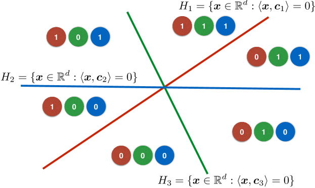
The second point of Th. 1 can be interpreted as follows: Pick a binary matrix $\bm{{B}}$ and treat each of the $n$ columns $\bm{{B}}_{j}$ as the labels of a binary classification problem $P_{j}$ on $m$ points. We can find data points $\bm{{x}}_{1},\dots,\bm{{x}}_{m}$ and affine hyperplanes $H_{1},\dots,H_{n}$ in $\mathbb{R}^{d}$ which solve all linear classification problems $P_{j}$ without error if and only if the rounding rank of $\bm{{B}}$ is at most $d$. We then interpret the $\bm{{x}}_{i}$ as data points and the $\bm{{c}}_{j}$ as feature weights. Rounding rank decompositions thus describe the “best case” for multiple linear classification problems: if the rounding rank of $\bm{{B}}$ is $d$, then we need at least $d$ features to achieve perfect classification. In other words, we need to collect at least $\operatorname{rrank}(\bm{{B}})$ features (or attributes) to have a chance to classify perfectly. Similarly, if we employ dimensionality reduction, linear classification cannot be perfect if we reduce to less than $d$ dimensions.

Corollary 2 (informal).

Rounding rank provides a natural lower bound on how many features we need for linear classification. This provides us with lower bounds on data collection or dimensionality reduction.

II-D Comparison of the Ranks

We compare rounding rank with several well-known ranks. Many of the results in this subsection were obtained for sign rank in the communication complexity community; we present these results here in terms of rounding rank. To the best of our knowledge, we are the first to make the role of the rounding threshold explicit by introducing mixed matrices (see Prop. 5).

Boolean rank

For binary matrices $\bm{{L}}\in\{0,1\}^{m\times k}$ and $\bm{{R}}\in\{0,1\}^{n\times k}$, the Boolean matrix product $\bm{{L}}\circ\bm{{R}}^{T}$ is given by the $m\times n$ binary matrix with $[\bm{{L}}\circ\bm{{R}}^{T}]_{ij}=\bigvee_{\ell=1}^{k}(\bm{{L}}_{ik}\land\bm{{R}}_{jk})$ for all entries $i,j$. The Boolean rank of a binary matrix $\bm{{B}}$, denoted $\operatorname{brank}(\bm{{B}})$, is the smallest $k\in\mathbb{N}$ s.t. there exist $\bm{{L}}\in\{0,1\}^{m\times k}$ and $\bm{{R}}\in\{0,1\}^{n\times k}$ with $\bm{{B}}=\bm{{L}}\circ\bm{{R}}^{T}$ [27]. The rounding rank is a lower bound on the Boolean rank.

Lemma 3.

$\operatorname{rrank}(\bm{{B}})\leq\operatorname{brank}(\bm{{B}})$.

Proof.

Let $\operatorname{brank}(\bm{{B}})=k$. Then there exist matrices $\bm{{L}}\in\{0,1\}^{m\times k}$ and $\bm{{R}}\in\{0,1\}^{n\times k}$ s.t. $\bm{{B}}=\bm{{L}}\circ\bm{{R}}^{T}$. If we use the algebra of $\mathbb{R}$, we get $[\bm{{L}}\bm{{R}}^{T}]_{ij}\geq\frac{1}{2}$ iff $\bm{{B}}_{ij}=1$. This implies $\operatorname{round}(\bm{{L}}\bm{{R}}^{T})=\bm{{B}}$ and $\operatorname{rrank}(\bm{{B}})\leq k=\operatorname{brank}(\bm{{B}})$. ∎

Real rank

Comparing rounding rank and real rank, we observe that $\bm{{B}}=\operatorname{round}(\bm{{B}})$ for all binary matrices $\bm{{B}}$. Hence,

$$\operatorname{rrank}(\bm{{B}})\leq\operatorname{rank}(\bm{{B}}).$$

This is in contrast to the relationship between Boolean rank and standard rank, which cannot be compared (i.e. neither serves as a lower bound to the other) [28].

Note that the rounding rank can be much lower than both real and Boolean rank. For example, the $n\times n$ “upper triangle matrix” with 1’s on the main diagonal and above has real and Boolean rank $n$, but rounding rank $1$ (see Th. 11). As another example, we show in Section -A in the appendix that the $n\times n$ identity matrix has rounding rank 2 for all $n\geq 3$. In fact, while we know that a real-valued $n\times n$ matrix can have rank up to $n$, the situation is different for rounding rank: On the one hand, for large enough $n$, all $n\times n$ matrices $\bm{{B}}$ have $\operatorname{rrank}(\bm{{B}})\leq(\frac{1}{2}+o(1))n$ [2, Cor. 1.2]. On the other hand, for each $n$, there exist $n\times n$ matrices with $\operatorname{rrank}(\bm{{B}})\geq\frac{n}{32}$, i.e., the rounding rank can indeed be linear in $n$ [2, Cor. 1.2].

It is well-known that real-valued matrices with all entries picked uniformly at random from some bounded proper interval have full standard rank with probability 1. For rounding rank, an $n\times n$ binary matrix sampled uniformly at random has rounding rank $\Omega(n)$ with high probability (see the proof of Cor. 1.2 in [2]). Hence, the rounding ranks of random binary matrices are expected to be large. The real-world data matrices in our experiments often had small rounding ranks, though.

A lower bound on the rounding rank of a binary matrix $\bm{{B}}$ can be derived from the singular values of the sign matrix $\bm{{B}}^{\pm}$.

Proposition 4.

Let $r=\operatorname{rank}(\bm{{B}}^{\pm})$ and let $\sigma_{1}(\bm{{B}}^{\pm})\geq\dots\geq\sigma_{r}(\bm{{B}}^{\pm})>0$ be the non-zero singular values of $\bm{{B}}^{\pm}$. Then

$$(\operatorname{rrank}_{0}(\bm{{B}})+1)\sum_{i=1}^{\operatorname{rrank}_{0}(\bm{{B}})}\sigma_{i}^{2}(\bm{{B}}^{\pm})\geq mn.$$

Prop. 4 is a slight modification of a result in [17, Th. 5] and we give the proof in the appendix.

Role of rounding threshold

We compare the rounding ranks of a fixed matrix for different rounding thresholds. We call a binary matrix mixed, if it contains no all-zero and no all-one columns (or rows).

Proposition 5.

For any $\bm{{B}}$ and arbitrary $\tau\neq\tau^{\prime}\in\mathbb{R}$, $\operatorname{rrank}_{\tau}(\bm{{B}})$ and $\operatorname{rrank}_{\tau^{\prime}}(\bm{{B}})$ differ by at most $1$. If additionally $\tau,\tau^{\prime}\neq 0$, $\operatorname{rrank}_{\tau}(\bm{{B}})=\operatorname{rrank}_{\tau^{\prime}}(\bm{{B}})$ if $\operatorname{sign}(\tau)=\operatorname{sign}(\tau^{\prime})$ or if $\bm{{B}}$ is mixed.

To prove Prop. 5 we need Lem. 6 below. The lemma is implied by the Hyperplane Separation Theorem [10, p. 46], and we prove it in the appendix.

Lemma 6.

Let $A$ and $B$ be two disjoint nonempty convex sets in $\mathbb{R}^{d}$, one of which is compact. Then for all nonzero $c\in\mathbb{R}$, there exists a nonzero vector $\bm{{v}}\in\mathbb{R}^{d}$, such that $\langle\bm{{x}},\bm{{v}}\rangle>c$ and $\langle\bm{{y}},\bm{{v}}\rangle<c$ for all $\bm{{x}}\in A$ and $\bm{{y}}\in B$.

Proof of Prop. 5.

First claim: Let $\tau,\tau^{\prime}\in\mathbb{R}$ be arbitrary and pick $k\in\mathbb{N}$, $\bm{{L}}\in\mathbb{R}^{m\times k}$, $\bm{{R}}\in\mathbb{R}^{n\times k}$ such that $\operatorname{round}_{\tau}(\bm{{L}}\bm{{R}}^{T})=\bm{{B}}$. Set $c=\tau^{\prime}-\tau$, then

$$\bm{{B}}_{ij}=\operatorname{round}_{\tau}([\bm{{L}}\bm{{R}}^{T}]_{ij})=\operatorname{round}_{\tau^{\prime}}([\bm{{L}}\bm{{R}}^{T}]_{ij}+c).$$

Set $\bm{{L}}^{\prime}=\begin{pmatrix}\bm{{L}}&c\mathbf{1}\end{pmatrix}$ and $\bm{{R}}^{\prime}=\begin{pmatrix}\bm{{R}}&\mathbf{1}\end{pmatrix}$, where $\mathbf{1}$ denotes the all-one vector. Then $\operatorname{round}_{\tau^{\prime}}(\bm{{L}}^{\prime}\bm{{R}}^{\prime T})=\bm{{B}}$ and thus $\operatorname{rrank}_{\tau^{\prime}}(\bm{{B}})\leq k+1$.

Second claim: Without loss of generality, assume that $\bm{{B}}$ contains no all-zero and no all-one columns (otherwise tranpose the matrix). Let $\tau,\tau^{\prime}\neq 0$ and let $k$ and $\bm{{L}}\bm{{R}}^{T}$ be as before. If $\operatorname{sign}(\tau)=\operatorname{sign}(\tau^{\prime})$, set $c=\tau^{\prime}/\tau>0$ and $\bm{{R}}^{\prime}=c\bm{{R}}$. Then $\operatorname{round}_{\tau}(\bm{{L}}\bm{{R}})=\operatorname{round}_{\tau^{\prime}}(\bm{{L}}\bm{{R}}^{\prime})$ by construction so that $\operatorname{rrank}_{\tau^{\prime}}(\bm{{B}})\leq k$. By reversing the roles of $\tau$ and $\tau^{\prime}$ in the argument, we establish $\operatorname{rrank}_{\tau}(\bm{{B}})=\operatorname{rrank}_{\tau^{\prime}}(\bm{{B}})$.

Suppose $\tau,\tau^{\prime}\neq 0$ (not necessarily of same sign) and let $\bm{{B}}$ be mixed. We now treat the rows of $\bm{{L}}$ as points $\bm{{L}}_{1},\dots,\bm{{L}}_{m}$ in $\mathbb{R}^{k}$ and show that there exists an $n\times k$ matrix $\bm{{R}}^{\prime}$ consisting of normal vectors of affine hyperplanes in $\mathbb{R}^{k}$ in its rows such that the hyperplanes separate the points with rounding threshold $\tau^{\prime}$, thereby establishing $\operatorname{rrank}_{\tau^{\prime}}(\bm{{B}})\leq\operatorname{rrank}_{\tau}(\bm{{B}})$. Again, by reversing the roles of $\tau$ and $\tau^{\prime}$, we obtain equality. To construct the $j$’th row of $\bm{{R}}^{\prime}$, let $C_{j}=\{\bm{{L}}_{i}:\bm{{B}}_{ij}=1\}$ and $\bar{C}_{j}=\{\bm{{L}}_{i}:\bm{{B}}_{ij}=0\}$. Notice that since $\bm{{B}}$ is mixed, both $C_{j}$ and $\bar{C}_{j}$ are non-empty. We observe that the convex hulls of $C_{j}$ and $\bar{C}_{j}$ are separated by the affine hyperplane with the $j$’th row of $\bm{{R}}$ as its normal vector and offset from the origin $\tau$. Thus, we apply Lem. 6 to obtain a vector $\bm{{r}}^{\prime}_{j}$ s.t. $\langle\bm{{r}}^{\prime}_{j},\bm{{c}}\rangle>\tau^{\prime}$ for all $\bm{{c}}\in C_{j}$ and $\langle\bm{{r}}^{\prime}_{j},\bar{}\bm{{c}}\rangle<\tau^{\prime}$ for all $\bar{}\bm{{c}}\in\bar{C}$. We set $\bm{{r}}^{\prime}_{j}$ to be the $j$’th row of $\bm{{R}}^{\prime}$. To obtain $\bm{{R}}^{\prime}$, we repeating this procedure for each of its $n$ rows. ∎

The above proof can be adopted to show that if $\bm{{B}}$ is mixed, even using a different (non-zero) rounding threshold for each row (or column) does not affect the rounding rank.

Non-negative rounding rank

While the gap between rank and non-negative rank can be arbitrarily large [6], for rounding rank and non-negative rounding rank this is not the case.

Proposition 7.

$\operatorname{rrank}^{+}_{\tau}(\bm{{B}})\leq\operatorname{rrank}_{\tau}(\bm{{B}})+2$.

This can be shown using ideas similar to the ones in [29] by a simple but lengthy computation. We give a proof in the appendix.

II-E Computational Complexity

The following proposition asserts that rounding rank is $\mathrm{NP}$-hard to compute regardless of the rounding threshold.

Proposition 8.

It is $\mathrm{NP}$-hard to decide if $\operatorname{rrank}_{0}(\bm{{B}})\leq k$ for all $k>2$. For $\tau\neq 0$, it is $\mathrm{NP}$-hard to decide if $\operatorname{rrank}_{\tau}(\bm{{B}})\leq k$ for all $k>1$.

For sign rank (i.e. $\tau=0$), this was proven in [9, Th. 1.2],[5, Sec. 3]. Moreover, Alon et al. [4] argue that computing the sign rank is equivalent to the existential theory of the reals. For $\tau\neq 0$, NP-hardness was proven in [24, Th. 10].

It is an open problem whether sign rank or rounding rank computation is in $\mathrm{NP}$. Assume we store a matrix $\bm{{A}}$ that achieves the rounding rank of $\bm{{B}}$ by representing all entries with rational numbers. The following proposition asserts that in general, the space needed to store a $\bm{{A}}$ can be exponential in the size of $\bm{{B}}$. Hence, the proposition rules out proving that computing rounding rank is in $\mathrm{NP}$ by nondeterministically guessing a matrix $\bm{{A}}$ of small rank and rounding it.

Proposition 9.

For all sufficiently large $n$, there exist $n\times n$ binary matrices $\bm{{B}}$ with $\operatorname{rrank}(\bm{{B}})=3$ s.t. for each matrix $\bm{{A}}$ with $\operatorname{rank}(\bm{{A}})=3$ and $\operatorname{round}(\bm{{A}})=\bm{{B}}$, it takes $\Theta(\exp(n))$ bits to store the entries of $\bm{{A}}$ using rational numbers.

Prop. 9 can be derived from the proof of [24, Th. 4].

Lemma 10.

The MinErrorRR-$k$ problem is $\mathrm{NP}$-hard to solve exactly. It is also $\mathrm{NP}$-hard to approximate within any polynomial-time computable factor.

Proof.

Both claims follow from Prop. 8. If in polynomial time we could solve the MinErrorRR-$k$ problem exactly or within any factor, then we could also decide if $\operatorname{rrank}(\bm{{B}})\leq k$ by checking if the result for MinErrorRR-$k$ is zero. ∎

III Computing the Rounding Rank

In this section, we provide algorithms approximating $\operatorname{rrank}(\bm{{B}})$ and for approximately solving the MinErrorRR-$k$ problem. The algorithms are based on some of the most common paradigms for algorithm design in data mining. The ProjLP algorithm makes use of randomized projections, R-SVD uses truncated SVD, L-PCA uses logistic PCA, and Asso is a Boolean matrix factorization algorithm. For each algorithm, we first discuss how to obtain an approximation to $\operatorname{rrank}(\bm{{B}})$ (in the form of an upper bound) and then discuss extensions to solve MinErrorRR-$k$.

Projection-based algorithm (ProjLP)

We first describe a Monte Carlo algorithm to decide whether $\operatorname{rrank}(\bm{{B}})\leq d$ for a given matrix $\bm{{B}}$ and $d\in\mathbb{N}$. The algorithm can output yes or unknown. If the algorithm outputs yes, it also produces a rounding rank decomposition. We use this algorithm for different values of $d$ to approximate $\operatorname{rrank}(\bm{{B}})$.

The decision algorithm is inspired by a simple observation: Considering an $m\times n$ binary matrix $\bm{{B}}$, we have $\bm{{B}}=\operatorname{round}(\bm{{B}}\bm{{I}})$, where $\bm{{I}}$ denotes the $n\times n$ identity matrix. We interpret each row $\bm{{B}}_{i}$ of $\bm{{B}}$ as a point in $\mathbb{R}^{n}$ and each column $\bm{{I}}_{j}$ of $\bm{{I}}$ as the normal vector of a hyperplane in $\mathbb{R}^{n}$. The hyperplane given by $\bm{{I}}_{j}$ separates the points $\bm{{B}}_{i}$ into the classes $C_{j}=\{\bm{{B}}_{i}:\bm{{B}}_{ij}=1\}$ and $\bar{C}_{j}=\{\bm{{B}}_{i}:\bm{{B}}_{ij}=0\}$ by the $j$’th column of $\bm{{B}}$, since $\bm{{B}}_{ij}=\operatorname{round}(\langle\bm{{B}}_{i},\bm{{I}}_{j}\rangle)$. The idea of ProjLP is to take the points $\bm{{B}}_{i}$ (the rows of $\bm{{B}}$) and to project them into lower-dimensional space $\mathbb{R}^{d}$, $d\ll n$, to obtain vectors $\bm{{L}}_{1},\dots,\bm{{L}}_{m}\in\mathbb{R}^{d}$. We use a randomized projection that approximately preserves the distances of the $\bm{{B}}_{i}$ and—if $\bm{{B}}$ has rounding rank at most $d$—try (or hope) to maintain the separability of the points by hyperplanes by doing so. Given the projected vectors in $\mathbb{R}^{d}$, we check separability by affine hyperplanes and find the corresponding normal vectors $\bm{{R}}_{1},\dots,\bm{{R}}_{n}$ using a linear program. If the $\bm{{L}}_{i}$ turn out to be separable, we have $\bm{{B}}_{ij}=\operatorname{round}(\langle\bm{{L}}_{i},\bm{{R}}_{j}\rangle)$ for all $i,j$ and thus $\bm{{B}}=\operatorname{round}(\bm{{L}}\bm{{R}}^{T})$, where $\bm{{L}}$ and $\bm{{R}}$ have the $\bm{{L}}_{i}$’s and $\bm{{R}}_{j}$’s in their rows, respectively. We conclude $\operatorname{rrank}(\bm{{B}})\leq d$ and output yes. If the $\bm{{L}}_{i}$ are not separable, no conclusions can be drawn and the algorithm outputs unknown.

The Johnson–Lindenstrauss Lemma [22] asserts that there exists a linear mapping $\bm{{A}}$ that projects points from a high-dimensional space into a lower-dimensional space while approximately preserving the distances. We use the projections proposed by Achlioptas [1] to obtain $\bm{{A}}$. We set $\bm{{L}}_{i}=\bm{{B}}_{i}\bm{{A}}$. The linear program (LP) to compute the normal vector $\bm{{R}}_{j}$ is

find $$\bm{{R}}_{j}\in\mathbb{R}^{d}$$

subject to $$\sum_{k=1}^{d}\bm{{L}}_{ik}\bm{{R}}_{jk}\geq\tau+\varepsilon \text{if }\bm{{B}}_{ij}=1,$$

$$\sum_{k=1}^{d}\bm{{L}}_{ik}\bm{{R}}_{jk}\leq\tau-\varepsilon \text{if }\bm{{B}}_{ij}=0.$$

We enforce strict separability by introducing an offset $\varepsilon>0$. In practice, we set $\varepsilon$ to the smallest positive number representable by the floating-point hardware. Notice that the LP only aims at finding a feasible solution; it has $m$ constraints and $d$ variables.

To approximate the rounding rank, we repeatedly run the above algorithm with increasing values of $d$ until it outputs yes; i.e., $d=1,2,\ldots$. Alternatively, we could use some form of binary search to find a suitable value of $d$. In practice, however, solving the LP for large values of $d$ slows down the binary search too much.

To solve MinErrorRR-$k$, we modify the LP of ProjLP to output an approximate solution. For this purpose, we introduce non-negative slack-variables $\bm{{c}}_{i}$ as in soft-margin SVMs to allow for errors, and an objective function that minimizes the $L_{1}$ norm of the slack variables. We obtain the following LP:

$$\min_{\begin{subarray}{c}\bm{{c}}\in\mathbb{R}_{\geq 0}^{m}\\ \bm{{R}}_{j}\in\mathbb{R}^{d}\end{subarray}} \sum_{i=1}^{m} \;\bm{{c}}_{i}$$

subject to $$\sum_{k=1}^{d} \;\bm{{L}}_{ik}\bm{{R}}_{jk}+\bm{{c}}_{i} \;\geq\; \tau+\varepsilon, \text{if }\bm{{B}}_{ij}=1,$$

$$\sum_{k=1}^{d} \;\bm{{L}}_{ik}\bm{{R}}_{jk}-\bm{{c}}_{i} \;\leq\; \tau-\varepsilon, \text{if }\bm{{B}}_{ij}=0.$$

Rounded SVD algorithm (R-SVD)

We use rounded SVD to approximate $\operatorname{rrank}(\bm{{B}})$. The algorithm is greedy and similar to the one in [14]. Given a binary matrix $\bm{{B}}$, the algorithm sets $k=1$. Then it computes the rank-$k$ truncated SVD of $\bm{{B}}$ and rounds it. If the rounded matrix and $\bm{{B}}$ are equal, it returns $k$, otherwise, it sets $k=k+1$ and repeats. The underlying reasoning is that the rank-$k$ SVD is the real-valued rank $k$ matrix minimizing the distance to $\bm{{B}}$ w.r.t. the Frobenius norm. Hence, also its rounded version should be “close” to $\bm{{B}}$.

To approximately solve MinErrorRR-$k$, we compute the truncated rank-$\ell$-SVD of $\bm{{B}}$ for all $\ell=1,\dots,k$ and return the rounded matrix with the smallest error.

Logistic Principal Component Analysis (L-PCA)

The logistic function $f(x)=\left(1+e^{-x}\right)^{-1}$ is a differentiable surrogate of the rounding function and it can be used to obtain a smooth approximation of the rounding.

L-PCA [31] models each $\bm{{B}}_{ij}$ as a Bernoulli random variable with success probability $f(\langle\bm{{L}}_{i},\bm{{R}}_{j}\rangle)$, where $\bm{{L}}\in\mathbb{R}^{m\times k}$ and $\bm{{R}}\in\mathbb{R}^{n\times k}$ are unknown parameters. Given $\bm{{B}}$ and $k\in\mathbb{N}$ as input, L-PCA obtains (approximate) maximum-likelihood estimates of $\bm{{L}}$ and $\bm{{R}}$. If each $f(\langle\bm{{L}}_{i},\bm{{R}}_{j}\rangle)$ is a good estimate of $\bm{{B}}_{ij}=1$, then $\lVert\bm{{B}}-\operatorname{round}(\bm{{L}}\bm{{R}}^{T})\rVert_{F}$ should be small.

To approximate the $\operatorname{rrank}(\bm{{B}})$, we run L-PCA on $\bm{{B}}$ for $k=1$ and check if $\operatorname{round}(\bm{{L}}\bm{{R}}^{T})=\bm{{B}}$. If this is the case, we return $k$, otherwise, we set $k=k+1$ and repeat.

To use L-PCA to compute an approximation of MinErrorRR-$k$, we simply run L-PCA and apply rounding.

Permutation algorithm (Permutation)

The only known algorithm to approximate the sign rank of a $n\times n$ matrix in polynomial time was given in [4]; it guarantees an upper bound within an approximation ratio of $O(n/\log n)$. By Prop. 5, we can use this method to approximate the rounding rank. The algorithm permutes the rows of the input matrix $\bm{{B}}$ s.t. the maximum number of bit flips over all columns is approximately minimized. It then algebraically approximates $\operatorname{rrank}(\bm{{B}})$ by evaluating a certain polynomial based on the occurring bit flips. The algorithm cannot solve the MinErrorRR-$k$ problem.

Nuclear norm algorithm (Nuclear)

The nuclear norm $\left\lVert\bm{{X}}\right\rVert_{*}$ of a matrix $\bm{{X}}$ is the sum of the singular values of $\bm{{X}}$ and is a convex and differentiable surrogate of the rank function of matrix. A common relaxation for minimum-rank matrix factorization is to minimize $\left\lVert\bm{{X}}\right\rVert_{*}$ instead of $\operatorname{rank}(\bm{{X}})$. In our setting, we obtain the following minimization problem:

$$\bm{{X}}^{*}= \operatorname*{arg\,min}_{\bm{{X}}\in\mathbb{R}^{m\times n}} \left\lVert\bm{{X}}\right\rVert_{*}$$

subject to $$\bm{{X}}_{ij}\geq\tau \text{if }\bm{{B}}_{ij}=1,$$

$$\bm{{X}}_{ij}<\tau \text{if }\bm{{B}}_{ij}=0.$$

This method has some caveats: While $\bm{{X}}^{*}$ must have small singular values, it may still have many. Additionally, by Prop. 9, some entries of a matrix $\bm{{A}}$ achieving the rounding rank might be extremely large. In such a case, some of the singular values of $\bm{{A}}$ must also be large, and consequently the nuclear norm of the matrix is large. Thus, $\bm{{X}}^{*}$ might have a too large rank. This algorithm cannot be extended to solve MinErrorRR-$k$.

IV Nested Matrices

A binary matrix is nested if we can reorder its columns such that after the reordering, the one-entries in each row form a contiguous segment starting from the first column [25]. Intuitively, nested matrices model subset/superset relationships between the rows and columns of a matrix. Such structures are, for example, found in presence/absence data of locations and species [25].

We show that nested matrices are exactly the matrices with non-negative rounding rank 1. Formally, a binary matrix $\bm{{B}}$ is directly nested if for each one-entry $\bm{{B}}_{ij}=1$, we have $\bm{{B}}_{i^{\prime}j^{\prime}}=1$ for all $i^{\prime}\in\{1,\dots,i-1\}$ and $j^{\prime}\in\{1,\dots,j-1\}$. A binary matrix $\bm{{B}}$ is nested if there exist permutation matrices $\bm{{P}}_{1}$ and $\bm{{P}}_{2}$, such that $\bm{{P}}_{1}\bm{{B}}\bm{{P}}_{2}$ is directly nested.

Theorem 11.

Let $\bm{0}\neq\bm{{B}}\in\{0,1\}^{m\times n}$. Then $\bm{{B}}$ is nested if and only if $\operatorname{rrank}^{+}(\bm{{B}})=1$.

Proof.

$\Rightarrow$: We reorder the rows and columns of $\bm{{B}}$ by the number of $1$s they contain in descending order. This gives us permutation matrices $\bm{{P}}_{1}$ and $\bm{{P}}_{2}$ s.t. $\bm{{B}}^{\prime}=\bm{{P}}_{1}\bm{{B}}\bm{{P}}_{2}$ is directly nested. Set $\bm{{p}}=\bm{{B}}^{\prime}\bm{1}$, i.e., $\bm{{p}}$ is the vector containing the row sums of $\bm{{B}}^{\prime}$. Then for $\bm{{l^{\prime}}}$ and $\bm{{r^{\prime}}}$ with $\bm{{l}}^{\prime}_{i}=2^{\bm{{p}}_{i}-1}$ and $\bm{{r}}^{\prime}_{j}=2^{-j}$, $\bm{{B}}^{\prime}=\operatorname{round}(\bm{{l}}^{\prime}\cdot(\bm{{r}}^{\prime})^{T})$. Setting $\bm{{l}}=\bm{{P}}_{1}^{T}\bm{{l}}^{\prime}$ and $\bm{{r}}=\bm{{P}}_{2}\bm{{r}}^{\prime}$, we get $\bm{{B}}=\operatorname{round}(\bm{{l}}\cdot\bm{{r}}^{T})$. Hence, we have $\operatorname{rrank}(\bm{{B}})=1$.

$\Leftarrow$: Let $\bm{{l}}\geq 0$ and $\bm{{r}}\geq 0$ be s.t. $\bm{{B}}=\operatorname{round}(\bm{{l}}\bm{{r}}^{T})$. Then there exist permutation matrices $\bm{{P}}_{1}$ and $\bm{{P}}_{2}$ s.t. for $\bm{{l}}^{\prime}=\bm{{P}}_{1}\bm{{l}}$ we have $\bm{{l}}_{1}^{\prime}\geq\dots\geq\bm{{l}}_{m}^{\prime}$ and for $\bm{{r}}^{\prime}=\bm{{P}}_{2}^{T}\bm{{r}}$ we have $\bm{{r}}_{1}^{\prime}\geq\dots\geq\bm{{r}}_{n}^{\prime}$. Set $\bm{{B}}^{\prime}=\operatorname{round}(\bm{{l}}^{\prime}(\bm{{r}}^{\prime})^{T})$ and observe $\bm{{l}}_{i}^{\prime}\bm{{r}}_{j}^{\prime}\geq\bm{{l}}_{i+1}^{\prime}\bm{{r}}_{j}^{\prime}$ for all $i,j$. Therefore, for each entry of $\bm{{B}}^{\prime}$, $\bm{{B}}^{\prime}_{ij}=\operatorname{round}(\bm{{l}}_{i}^{\prime}\bm{{r}}_{j}^{\prime})\geq\operatorname{round}(\bm{{l}}_{i+1}^{\prime}\bm{{r}}_{j}^{\prime})=\bm{{B}}^{\prime}_{(i+1)j}$. Similarly, $\bm{{B}}^{\prime}_{ij}=\operatorname{round}(\bm{{l}}_{i}^{\prime}\bm{{r}}_{j}^{\prime})\geq\operatorname{round}(\bm{{l}}_{i}^{\prime}\bm{{r}}_{j+1}^{\prime})=\bm{{B}}^{\prime}_{i(j+1)}$. Therefore, $\bm{{B}}^{\prime}$ is directly nested. We conclude that $\bm{{B}}=\bm{{l}}\bm{{r}}^{T}$ is nested since $\bm{{B}}=\operatorname{round}(\bm{{l}}\bm{{r}}^{T})=\bm{{P}}_{1}^{T}\operatorname{round}(\bm{{P}}_{1}(\bm{{l}}\bm{{r}}^{T})\bm{{P}}_{2})\bm{{P}}_{2}^{T}=\bm{{P}}_{1}^{T}\bm{{B}}^{\prime}\bm{{P}}_{2}^{T}$. ∎

Binary matrices with rounding rank 1 are also closely related to nested matrices.

Proposition 12.

Let $\bm{0}\neq\bm{{B}}\in\{0,1\}^{m\times n}$. The following statements are equivalent:

1. $\operatorname{rrank}(\bm{{B}})=1$.

2. there exist permutation matrices $\bm{{P}}_{1}$ and $\bm{{P}}_{2}$ and nested matrices $\bm{{B}}_{1}$ and $\bm{{B}}_{2}$, such that

   $$\bm{{B}}=\bm{{P}}_{1}\begin{pmatrix}\bm{{B}}_{1}&0\\ 0&\bm{{B}}_{2}\end{pmatrix}\bm{{P}}_{2}.$$

The proof is in the appendix.

Algorithms

Mannila and Terzi [25] introduced the Bidirectional Minimum Nestedness Augmentation (BMNA) problem: Given a binary matrix $\bm{{B}}$, find the nested matrix $\bm{{A}}$ which minimizes $\left\lVert\bm{{B}}-\bm{{A}}\right\rVert_{F}$. We will discuss three algorithms to approximately solve this problem.

[25] gave an algorithm, MT, which approximates a solution for the BMNA problem by iteratively eliminating parts of the matrix that violate the nestedness.

Next, we propose a alternating minimization algorithm, NNRR1, which exploits Th. 11. NNRR1 maintains two vectors $\bm{{l}}\in\mathbb{R}_{\geq 0}^{m}$ and $\bm{{r}}\in\mathbb{R}_{\geq 0}^{n}$ and iteratively minimizes the error $\lVert\bm{{B}}-\operatorname{round}(\bm{{l}}\cdot\bm{{r}}^{T})\rVert_{F}$. It starts by fixing $\bm{{r}}$ and updates $\bm{{l}}$, such that the error is minimized. Then $\bm{{l}}$ is fixed and $\bm{{r}}$ is updated. This procedure is repeated until the error stops reducing or we have reached a certain number of iterations.

We describe an update of $\bm{{l}}$ for fixed $\bm{{r}}$; updating $\bm{{r}}$ for given $\bm{{l}}$ is symmetric. Observe that changing entry $\bm{{l}}_{i}$ only alters the $i$’th row of $\bm{{A}}=\bm{{l}}\cdot\bm{{r}}^{T}$, and consequently $\bm{{A}}_{i}$ is not affected by any $\bm{{l}}_{k}$ with $k\neq i$. Hence, we only describe the procedure for updating $\bm{{l}}_{i}$. Define the set $V_{i}=\{\bm{{r}}_{j}:\bm{{B}}_{ij}=1\}$ of all values of $\bm{{r}}$ where $\bm{{B}}_{i}$ is non-zero. We make the following observations: If we set $\bm{{l}}_{i}<\frac{1}{2\max(\bm{{r}})}$, then $\bm{{A}}_{i}$ only contains zeros after the update. If $\frac{1}{2\max(\bm{{r}})}<\bm{{l}}_{i}<\frac{1}{2\max(V_{i})}$, then after the update all non-zeros of $\bm{{A}}_{i}$ will be in entries where $\bm{{B}}_{i}$ has a zero. If $\bm{{l}}>\frac{1}{2\min(V_{i})}$, we add too many $1$s to $\bm{{A}}_{i}$. Thus, all values that we need to consider for updating $\bm{{l}}_{i}$ are $\frac{1}{2\max(\bm{{r}})}$ and the values in $\{\frac{1}{2v}:v\in V_{i}\}$. The algorithm tries all possible values for $\bm{{l}}_{i}$ exhaustively and computes the error at each step.

We can also use the results of MT as initialization for NNRR1: We run MT and obtain a nested matrix $\bm{{B}}$. Now we use the construction from step 1 of the proof of Th. 11 to obtain $\bm{{l}}$ and $\bm{{r}}$ with $\bm{{B}}=\operatorname{round}(\bm{{l}}\bm{{r}}^{T})$, and try to improve using NNRR1.

Finally, we can use R-SVD to solve the BMNA problem approximately. By the Perron–Frobenius Theorem [21, Ch. 8.4], the principal left and right singular vectors of a non-negative matrix are also non-negative. Hence we may use the R-SVD algorithm to obtain the rank-$1$ truncated SVD and round. By Th. 11, the result must be nested.

V Experiments

We conducted an experimental study on synthetic and real-world datasets to evaluate the relative performance of each algorithm for estimating the rounding rank or for MinErrorRR-$k$.

V-A Implementation Details

For L-PCA, we used the implementation by the authors of [31]. We implemented MT and Permutation in C and all other algorithms in Matlab. For Nuclear, we used the CVX package with the SeDuMi solver [20]. For solving the linear programs in ProjLP, we used Gurobi.

Due to numerical instabilities, Nuclear often returned a matrix with only positive singular values (i.e. of full rank). We countered this by zeroing the smallest singular values of the returned matrix that did not affect to the result of the rounding.

All experiments were conducted on a computer with eight Intel Xeon E5530 processors running at 2.4 GHz and 48 GB of main memory. All our algorithms and the synthetic data generators are available online.​

V-B Results With Synthetic Data

We start by studying the behavior of the algorithms under controlled synthetic datasets.

V-B1 Data generation

We generated synthetic data by sampling two matrices $\bm{{L}}\in\mathbb{R}^{m\times k}$ and $\bm{{R}}\in\mathbb{R}^{n\times k}$ and then rounding their product to obtain $\bm{{B}}=\operatorname{round}_{\tau}(\bm{{L}}\bm{{R}}^{T})$ with rounding rank at most $k$. The actual rounding rank of $\bm{{B}}$ can be lower, however, because there may be matrices $\bm{{L}}^{\prime}\in\mathbb{R}^{m\times k^{\prime}}$ and $\bm{{R}}^{\prime}\in\mathbb{R}^{n\times k^{\prime}}$ with $k^{\prime}<k$ and $\operatorname{round}_{\tau}(\bm{{L}}^{\prime}\bm{{R}}^{\prime T})=\bm{{B}}$. (In fact, we sometimes found such matrices.) In some experiments, we additionally applied noise by flipping elements selected uniformly at random. We report as noise level $p$ the ratio of the number of flipped elements to the number of non-zeros in the original noise-free matrix.

We sampled every element of $\bm{{L}}$ and $\bm{{R}}$ i.i.d. using two families of distributions: uniform and normal distribution. For both distributions, we first pick a desired expected value $\mu=\mathbb{E}[(\bm{{L}}\bm{{R}}^{T})_{ij}]$ of each entry in $\bm{{L}}\bm{{R}}^{T}$. We then parameterize the distributions such that the expected value for an element of $\bm{{L}}$ or $\bm{{R}}$ is $q=\sqrt{\mu/k}$. For the normal distribution, we set the variance to $1$, and for the uniform distribution, we sampled from range $[q-1/2,q+1/2]$.

We generated two sets of matrices. In the first set, the matrices were very small, and it was used to understand the behavior of the slower algorithms. In the second set, the matrices were medium-sized, to give us more realistic-sized data, but we could use only some of the methods with these data. When generating the data, we varied four different parameters: number of rows $m$, the planted rank $k$, the expected value $\mu$, and the level of noise $p$. In all experiments, we varied one of these parameters, while keeping the others fixed. We generated all datasets with rounding threshold $\tau=1/2$. For the small data, we used $n=100$ columns and the number of rows varied from $60$ to $220$ with steps of $40$ with the default value being $n=100$. The rank $k$ in the small matrices varied from $5$ to $30$ with steps of $5$, default being $k=10$; the expected value $\mu$ varied from $0.1$ to $0.7$ with $0.1$ steps (default was $\mu=0.5$); the noise level $p$ varied from $0.05$ to $0.5$ with steps of $0.05$, and by default we did not apply any noise. We generated ten random matrices with each parameter setting to test the variation of the results.

For the medium-sized matrices, we used $n=300$ columns and the number of rows varied from $400$ to $600$ with steps of $50$ the default being $m=500$; the planted rank $k$ varied from $40$ to $100$ with default value $k=60$; the expected value and the noise were as with the small data. We generated five random matrices with each parameter setting.

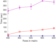
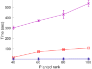
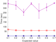
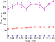
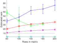
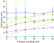
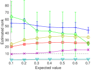
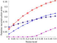
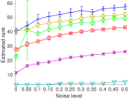
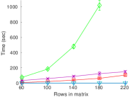
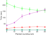
V-B2 Rounding rank

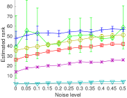
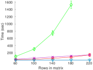
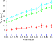
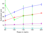
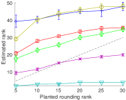
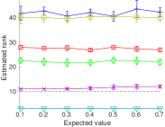
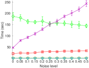
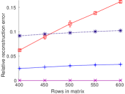
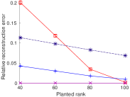
In our first set of experiments, we studied the performance of the different algorithms for estimating the rounding rank. The results for the small synthetic datasets are summarized in Fig. 2. The results are given for the uniformly distributed factor matrices; the results with normally distributed factors were largely similar and are postponed to the appendix.

Uniform dist.

(a) Rank, vary $m$

(b) Rank, vary $k$

(c) Rank, vary $\mu$

(d) Rank, vary $p$

Time

(e) Time, vary $m$

(f) Time, vary $k$

(g) Time, vary $\mu$

(h) Time, vary $p$

Figure 2: Estimated rounding ranks and running times on small synthetic data varying different parameters. The top row gives estimated rank for uniformly distributed factor matrices and the bottom row shows running times. Permutation can only run on square matrices and was excluded from the “vary $m$” experiments. All data points are averages over 10 random matrices and the width of the error bars is twice the standard deviation.

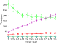
We used ProjLP, Nuclear, R-SVD, and L-PCA. We also used Permutation in all experiments except when we varied the number of rows (Permutation only works with square matrices). We also computed a lower bound Spectral LB on $\operatorname{rrank}_{0}$ using Prop. 4. Finally, in experiments with no noise, we also plot the planted rank (inner dimension of the factor matrices), which acts as an upper bound of the actual rounding rank.

As can be seen from Fig. 2, the estimated lower bound is almost always less than 3, even when the data contains significant amounts of noise. It seems reasonable to assume that the true rounding rank of the data is therefore closer to the upper bound of our planted rank than the estimated lower bound given by Spectral LB.

Of the algorithms tested here, ProjLP, and Permutation are the only ones that aim directly to find the rounding rank, with Permutation being the only one with approximation guarantees (albeit weak ones). Our experiments show that Permutation is not competitive to most other methods; good theoretical properties do not ensure a good practical behavior. ProjLP performs much better, being typically the second-best method. R-SVD is commonly employed in the literature, but our experiments show clearly that for computing the rounding rank, it is not recommended.

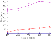
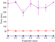
L-PCA consistently produced the smallest (i.e. best) rank estimate but it was also the second-slowest method. ProjLP, the second-best method for estimating the rank, was much faster. R-SVD often produced the worst estimates, but it is also the fastest method. The running times are broadly as expected: Nuclear has to solve a semidefinite programming problem, L-PCA solves iteratively dense least-squares problems, ProjLP only needs to solve linear equations, and R-SVD computes a series of orthogonal projections.

Varying the different parameters yielded mostly expected results with the most interesting result being how little the rank and noise had effect to the results. We assume that this is (at least partially) due to the robustness of the rounding rank: increasing the noise, say, might not have increased the rounding rank of the matrix. This is clearly observed when the rank is varied (Fig. 2(b)), where L-PCA actually obtains smaller rounding rank than the planted one.

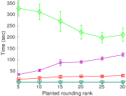
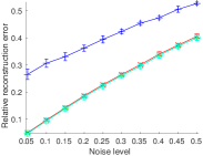
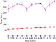
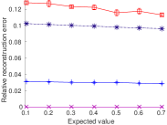
V-B3 Minimum-error decomposition

We now study the algorithms’ capability to return low-error fixed-rank decompositions. We leave out Permutation and Nuclear as they only approximate rounding rank. Instead, we add a method to compare against: T-SVD. It computes the standard truncated SVD, that is, we do not apply any rounding. T-SVD is used for providing a baseline: in principle, the methods that apply rounding should give better results as they utilize the added information that the final matrix must be binary. At the same time, however, the rounding procedure may emphasize small errors (e.g., incorrectly representing a $1$ with $0.49$ contributes $\approx 0.26$ to the sum of squares; after rounding, the contribution is $1$). We also tested the Asso [27] algorithm for Boolean matrix factorization (BMF). Like any BMF algorithm, Asso returns a rounding rank decomposition restricted to binary factor matrices. The performance of Asso’s approximations was so much worse than the performance of the other methods that we decided to omit it from the results.

To compare the algorithms, we use the relative reconstruction error, that is, the squared Frobenius norm of the distance between the data and its representation relative to the squared norm of the data. For all method except T-SVD, the relative reconstruction error agrees with the absolute number of errors divided by the number of non-zeros in the data.

Uniform dist.

(a) Error, vary $m$

(b) Error, vary $k$

(c) Error, vary $\mu$

(d) Error, vary $p$

Figure 3: Relative reconstruction errors on medium-sized synthetic data with uniformly distributed factors. The results of Asso are omitted as they were significantly worse than the other results. All data points are averages over 10 random matrices and the width of the error bars is twice the standard deviation.

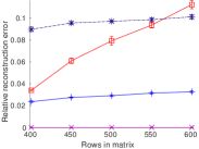
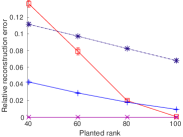
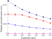
The results for these experiments are presented in Fig. 3. We only report the reconstruction with uniformly distributed factors: the running times were as with the above experiments, and the results with normally distributed factors were generally similar to the reported ones. The other results are in the appendix. As in the above experiments, L-PCA is the best method, and the slowest as well, taking sometimes an order of magnitude longer than ProjLP. The best all-rounder here, though, is the R-SVD method: it provided reasonable results and was by far the fastest method.

V-C Results with Real-World Data

We now turn our attention to real-world datasets. For these experiments we used only ProjLP, L-PCA, and R-SVD to estimate the rounding rank, and added T-SVD and Asso for the minimum-error decompositions.

Datasets

The basic properties of the datasets are listed in Tab. I. The Abstracts data set is a collection of project abstracts that were submitted to the National Science Foundation of the USA in applications for funding. The data is documents-by-terms matrix giving the appearance of terms in documents. The DBLP data is an authors-by-conferences matrix containing information who published where. The Paleo data set contains information about the locations at which fossils of certain species were found. It was fetched by [18] and preprocessed according to [19]. The Dialect data [11, 12] contains information about which linguistic features appear in the dialect spoken in various parts of Finland. The APJ dataset is a binary matrix containing access control rules from Hewlett-Packard [13].

Rounding rank

First we computed the upper bounds for the rounding ranks with the different methods. The results and running times are shown in Tab. I. As with the synthetic experiments, L-PCA is again giving the best results, followed by ProjLP and R-SVD, the latter of which returns often significantly worse results than the other two. In the running times the order is reversed, L-PCA taking orders of magnitude longer than ProjLP, which is still slower than R-SVD.

Table I: Upper bounds for rounding rank with $\tau=0.5$ for the real-world data. Known Boolean ranks from [7]. L-PCA did not finish on the Abstracts data in reasonable time.

	Dataset properties				Upper bounds on $\operatorname{rrank}$
Dataset	$m$	$n$	$\operatorname{rank}$	$\operatorname{brank}$	ProjLP	L-PCA	R-SVD
Abstracts	12841	4894	4893	–	449	–	4421
					(437h)	–	(9h)
APJ	2044	1164	455	453	29	9	443
					(151s)	(109min)	(35s)
DBLP	19	6980	19	19	12	11	19
					(46s)	(77min)	(2s)
Dialect	1334	506	506	–	91	78	445
					(527s)	(54h)	(17s)
Paleo	124	139	123	–	26	13	68
					(10s)	(271s)	(1s)

Note that the estimated rounding ranks in Tab. I are significantly less than the respective normal or Boolean ranks. For example, for the APJ data, the normal rank is $455$, the Boolean rank is $453$, but L-PCA shows that the rounding rank is at most $9$. Similarly, the normal and Boolean ranks for DBLP are $19$, while the rounding rank is no more than $11$. In most cases, the rounding rank is about an order of magnitude smaller than the real rank. This shows that the expressive power of the methods significantly increases by applying the rounding.

Minimum-error decompositions

The relative reconstruction errors for the real-world datasets together with running times are presented in Tab. II. Again, L-PCA is often—but not always—the best method, especially with higher ranks. Again, the running time was high though. An exception to this is the Abstracts data, where L-PCA is in fact faster than ProjLP (although it is still extremely slow). Again, ProjLP is often the second-best, and more consistently so with higher ranks.

Table II: Reconstruction errors relative to the number of non-zeros and running times in real-world data.

	Abstracts			APJ			DBLP			Dialect			Paleo
$k=$	$10$	$50$	$100$	$5$	$10$	$15$	$5$	$10$	$15$	$10$	$30$	$50$	$5$	$10$	$20$
Relative reconstruction error
ProjLP	$1.152$	$1.091$	$0.842$	$\mathbf{0.626}$	$0.302$	$0.099$	$0.408$	$0.060$	$0.003$	$0.378$	$0.130$	$0.036$	$0.701$	$0.360$	$0.037$
L-PCA	$0.993$	$0.863$	$\mathbf{0.459}$	$0.631$	$\mathbf{0.194}$	$\mathbf{0.034}$	$\mathbf{0.150}$	$\mathbf{0.003}$	$\mathbf{0.000}$	$\mathbf{0.200}$	$\mathbf{0.031}$	$\mathbf{0.002}$	$0.552$	$\mathbf{0.089}$	$\mathbf{0.000}$
R-SVD	$0.995$	$0.937$	$0.843$	$0.641$	$0.611$	$0.573$	$0.488$	$0.225$	$0.058$	$0.258$	$0.137$	$0.094$	$0.697$	$0.516$	$0.260$
T-SVD	$\mathbf{0.917}$	$\mathbf{0.838}$	$0.766$	$0.640$	$0.596$	$0.559$	$0.382$	$0.198$	$0.064$	$0.212$	$0.120$	$0.089$	$\mathbf{0.515}$	$0.410$	$0.283$
Asso	$0.988$	$0.971$	$0.960$	$0.663$	$0.637$	$0.603$	$0.531$	$0.347$	$0.187$	$0.442$	$0.358$	$0.333$	$0.793$	$0.706$	$0.602$
Running time (seconds)
ProjLP	$9627$	$27201$	$72956$	$54$	$64$	$63$	$12$	$13$	$12$	$26$	$83$	$169$	$2$	$2$	$2$
L-PCA	$675$	$17849$	$39954$	$39$	$235$	$297$	$98$	$114$	$109$	$96$	$166$	$218$	$11$	$12$	$17$
R-SVD	$3$	$6$	$13$	$1$	$1$	$1$	$1$	$1$	$1$	$1$	$1$	$1$	$1$	$1$	$1$
T-SVD	$2$	$6$	$13$	$1$	$1$	$1$	$1$	$1$	$1$	$1$	$1$	$1$	$1$	$1$	$1$
Asso	$2366$	$11701$	$23023$	$8$	$17$	$23$	$29$	$52$	$75$	$49$	$145$	$238$	$1$	$1$	$1$

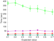
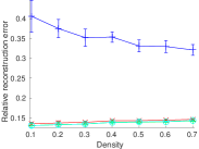
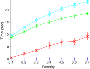
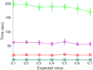
V-D Nestedness

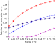
Here we studied the possibility to use the non-negative rounding rank-1 decomposition to solve the BMNA problem. For these purposes, we generated nested matrices, perturbed them with noise, and tried to find the closest nested matrix using MT, NNRR1, their combination MT+NNR1, and R-SVD. All nested matrices were $200\text{-by-}300$ and we varied the density of the data (from $0.1$ to $0.7$ with steps of $0.1$) and the noise level (from $0.05$ to $0.5$ with steps of $0.05$). A default density of $\mu=0.5$ was used when the noise was varied, and noise level $p=0.15$ was used when the density was varied.

Our results are shown in Fig. 4. MT and NNRR1 produced similar results, with MT being slightly better. The combined MT+NNR1 is no better than MT, and R-SVD is significantly worse. In the running times, though, we see that MT takes much more time than the other approaches.

(a) Error, vary density

(b) Error, vary noise level

(c) Time, vary density

(d) Time, vary noise

Figure 4: Relative reconstruction errors and running times on nested data. The running times for MT+NNR1 exclude the running time of the MT algorithm. All data points are averages over 10 random matrices and the width of the error bars is twice the standard deviation.

VI Conclusions

Rounding rank is a natural way to characterize the commonly-applied rounding procedure. Rounding rank has some significant differences to real rank: for example, restricting the factor matrices to be non-negative has almost no consequences to rounding rank. Rounding rank provides a robust definition of an intrinsic dimension of a data, and as we saw in the experiments, real-world data sets can have surprisingly small rounding ranks. At the same time, rounding rank-related problems appear naturally in various different fields of data analysis; for example, the connection to nested matrices is somewhat surprising, and allowed us to develop new algorithms for the BMNA problem.

Unfortunately, computing the rounding rank, and the related minimum-error decomposition, is computationally very hard. We have studied a number of algorithms—based on common algorithm design paradigms in data mining—in order to understand how well they behave in our problems. None of the tested algorithms emerges as a clear winner, though.

The most obvious future research direction is to find better algorithms that aim directly for good rounding rank decompositions and scale to larger data sizes. Another question is if the factors obtained by a rounding rank decomposition reveal interpretable insights into the data. The connections of rounding rank to other problems also propose natural follow-up questions. For example, communities in graphs are often nested (sub-)matrices [26]. Could rounding rank decompositions be used to find non-clique-like communities?

We will first provide proofs of the lemmata and propositions omitted in the main text, and then provide additional results of our experimental evaluation.

-A Identity Matrices Have Rounding Rank 2

For $n\geq 3$, let $\bm{{I}}_{n}\in\mathbb{R}^{n\times n}$ be the identity matrix. From Proposition 12 we get that $\operatorname{rrank}(\bm{{I}}_{n})>1$, since the identity matrix is not nested. We look at the matrix

$$\bm{{A}} =\begin{pmatrix}1&-\frac{1}{2}\\ 2^{-1}&-\frac{1}{2}4^{-1}\\ \vdots&\vdots\\ 2^{-n+1}&-\frac{1}{2}4^{-n+1}\end{pmatrix}\begin{pmatrix}1&2&\ldots&2^{n-1}\\ 1&4&\ldots&4^{n-1}\end{pmatrix}$$

$$=\begin{pmatrix}1-\frac{1}{2}&2-\frac{4}{2}&4-\frac{16}{2}&\cdots\\ \frac{1}{2}-\frac{1}{8}&1-\frac{4}{8}&2-\frac{16}{8}&\cdots\\ \frac{1}{4}-\frac{1}{32}&\frac{1}{2}-\frac{4}{32}&1-\frac{16}{32}&\cdots\\ \vdots&\vdots&\vdots&\ddots\end{pmatrix},$$

and observe that $\bm{{A}}_{ij}=\frac{1}{2}$, if $i=j$, and $\bm{{A}}_{ij}<\frac{1}{2}$, otherwise. Thus, we get $\operatorname{round}(\bm{{A}})=\bm{{I}}_{n}$ and therefore $\operatorname{rrank}(\bm{{I}}_{n})=2$.

-B Proof of Proposition 4

[17] proved a lower bound for sign rank.

Lemma A.1 ([17, Th. 5]).

Let $\bm{{B}}\in\{-1,+1\}^{m\times n}$. Let $r=\operatorname{rank}(\bm{{B}})$ and let $\sigma_{1}(\bm{{B}})\geq\dots\geq\sigma_{r}(\bm{{B}})>0$ be the singular values of $\bm{{B}}$. Denote the sign rank of $\bm{{B}}$ by $d$. Then

$$d\sum_{i=1}^{d}\sigma_{i}^{2}(\bm{{B}})\geq mn.$$

We use the previous lemma to prove a lower bound on rounding rank.

Proposition 4 (again).

Let $r=\operatorname{rank}(\bm{{B}}^{\pm})$ and let $\sigma_{1}(\bm{{B}}^{\pm})\geq\dots\geq\sigma_{r}(\bm{{B}}^{\pm})>0$ be the singular values of $\bm{{B}}^{\pm}$. Then

$$(\operatorname{rrank}_{0}(\bm{{B}})+1)\sum_{i=1}^{\operatorname{rrank}_{0}(\bm{{B}})}\sigma_{i}^{2}(\bm{{B}}^{\pm})\geq mn.$$

Proof.

As argued in the main text, $\operatorname{rrank}_{0}(\bm{{B}})\leq\operatorname{srank}(\bm{{B}})$ for all $\bm{{B}}$. This implies

$$\sum_{i=1}^{\operatorname{srank}(\bm{{B}})}\sigma_{i}^{2}(\bm{{B}}^{\pm})\geq\sum_{i=1}^{\operatorname{rrank}_{0}(\bm{{B}})}\sigma_{i}^{2}(\bm{{B}}^{\pm}).$$

Using the previous lemma for sign rank and $\operatorname{rrank}_{0}(\bm{{B}})+1\geq\operatorname{srank}(\bm{{B}})$, we get

$$\operatorname{rrank}_{0}(\bm{{B}})+1 \geq\operatorname{srank}(\bm{{B}})$$

$$\geq\frac{mn}{\sum_{i=1}^{\operatorname{srank}(\bm{{B}})}\sigma_{i}(\bm{{B}}^{\pm})}$$

$$\geq\frac{mn}{\sum_{i=1}^{\operatorname{rrank}_{0}(\bm{{B}})}\sigma_{i}(\bm{{B}}^{\pm})}.$$

After multiplying with the denominator of the last equation, we obtain the desired result. ∎

-C Proof of Lemma 6

We revisit the Hyperplane Separation Theorem.

Hyperplane Separation Theorem [10, page 46].

Let $A$ and $B$ be two disjoint nonempty closed convex sets in $\mathbb{R}^{d}$, one of which is compact. Then there exists a nonzero vector $\bm{{v}}\in\mathbb{R}^{d}$ and real numbers $c_{1}<c_{2}$, such that $\langle\bm{{x}},\bm{{v}}\rangle>c_{2}$ and $\langle\bm{{y}},\bm{{v}}\rangle<c_{1}$ for all $\bm{{x}}\in A$ and $\bm{{y}}\in B$.

Now we prove Lemma 6 of the paper.

Lemma 6 (again).

Let $A$ and $B$ be two disjoint nonempty convex sets in $\mathbb{R}^{d}$, one of which is compact. Then for all $c\in\mathbb{R}\setminus\{0\}$ there exists a nonzero vector $\bm{{v}}\in\mathbb{R}^{d}$, such that $\langle\bm{{x}},\bm{{v}}\rangle>c$ and $\langle\bm{{y}},\bm{{v}}\rangle<c$ for all $\bm{{x}}\in A$ and $\bm{{y}}\in B$.

Proof.

Let $c\in\mathbb{R}\setminus\{0\}$ be arbitrary. We apply the Hyperplane Separation Theorem to $A$ and $B$ to obtain a vector $\bm{{v}}^{\prime}$ and numbers $c_{1}<c_{2}$ with $\langle\bm{{x}},\bm{{v}}^{\prime}\rangle>c_{2}$ and $\langle\bm{{y}},\bm{{v}}^{\prime}\rangle<c_{1}$ for all $\bm{{x}}\in A$ and all $\bm{{y}}\in B$. Now we consider three cases.

Case 1: $c_{1}\neq 0$ and $c_{2}\neq 0$ and $\operatorname{sign}(c_{1})=\operatorname{sign}(c_{2})$. We set $\alpha=c/c_{2}$ and $\bm{{v}}=\alpha\bm{{v}}^{\prime}$. Then we get for $\bm{{x}}\in A$:

$$\langle\bm{{x}},\bm{{v}}\rangle=\alpha\langle\bm{{x}},\bm{{v}}^{\prime}\rangle>\alpha c_{2}=c,$$

as well as for $\bm{{y}}\in B$:

$$\langle\bm{{y}},\bm{{v}}\rangle=\alpha\langle\bm{{y}},\bm{{v}}^{\prime}\rangle<\alpha c_{1}=\frac{c_{1}}{c_{2}}c<c,$$

where in the last inequality we used that $0<c_{1}/c_{2}<1$.

Case 2: $c_{1}\neq 0$ and $c_{2}\neq 0$ and $\operatorname{sign}(c_{1})\neq\operatorname{sign}(c_{2})$. Since the signs of $c_{1}$ and $c_{2}$ disagree, we have $c_{1}<0<c_{2}$. Thus, we can pick $c_{1}^{\prime}\in(0,c_{2})$ arbitrarily and still maintain all properties guaranteed by the Hyperplane Separation Theorem for $\bm{{v}}$, $c_{1}^{\prime}$ and $c_{2}$. Now we are in case 1.

Case 3: $c_{1}=0$ or $c_{2}=0$. We can pick numbers $d_{1},d_{2}\in(c_{1},c_{2})$ with $d_{1}<d_{2}$. Observe that both $d_{1}$ and $d_{2}$ are non-zero. Then we have $\langle\bm{{x}},\bm{{v}}^{\prime}\rangle>c_{2}>d_{2}$ and $\langle\bm{{y}},\bm{{v}}^{\prime}\rangle<c_{1}<d_{1}$ for all $\bm{{x}}\in A$ and all $\bm{{y}}\in B$. Now we can use case 1 for $\bm{{v}}^{\prime}$, $d_{1}$ and $d_{2}$. ∎

-D Proof of Proposition 7

The proof follows ideas of [29] and adds some details to achieve the non-negativity.

Proposition 7 (again).

Let $\bm{{B}}\in\{0,1\}^{m\times n}$ be a binary matrix. Then

$$\operatorname{rrank}(\bm{{B}})\leq\operatorname{rrank}_{+}(\bm{{B}})\leq\operatorname{rrank}(\bm{{B}})+2.$$

Proof.

The first inequality is trivial as the standard rounding rank is more general than the non-negative rounding rank.

The trickier part is the second inequality. The idea of the proof is to take points and hyperplanes achieving the rounding rank of the matrix and to project them into a higher dimensional space, where they are non-negative. This projection happens via an explicit construction, that gets somewhat technical.

Let $k=\operatorname{rrank}(\bm{{B}})$. Then by definition there exist matrices $\bm{{L}}\in\mathbb{R}^{m\times k}$ and $\bm{{R}}\in\mathbb{R}^{n\times k}$ with $\bm{{B}}=\operatorname{round}(\bm{{L}}\bm{{R}}^{T})$ for rounding threshold $\frac{1}{2}$. As before we will interpret the rows $\bm{{l}}_{1},\dots,\bm{{l}}_{m}$ of $\bm{{L}}$ as points in $\mathbb{R}^{k}$ and the rows $\bm{{r}}_{1},\dots,\bm{{r}}_{n}$ of $\bm{{R}}$ as normal vectors of affine hyperplanes in $\mathbb{R}^{k}$.

For each $\bm{{r}}_{j}=\left(\bm{{r}}_{j1},\dots,\bm{{r}}_{jk}\right)$, we set $\bm{{r}}_{j}^{\prime}=\left(\bm{{r}}_{j1},\dots,\bm{{r}}_{jk},-\frac{1}{2},\frac{1}{2}-\sum_{m=1}^{k}\bm{{r}}_{jm}\right)\in\mathbb{R}^{k+2}$ and observe that these vectors define hyperplanes in $\mathbb{R}^{k+2}$ containing the origin, i.e. we have $0\in\left\{\bm{{x}}\in\mathbb{R}^{k+2}:\langle\bm{{x}},\bm{{r}}_{j}^{\prime}\rangle=0\right\}$. We set $d_{j}=\max\{|\bm{{r}}_{jm}^{\prime}|:m=1,\dots,k+2\}$ and define $\bm{{r}}_{j}^{\prime\prime}=\frac{1}{2d_{j}}\bm{{r}}_{j}^{\prime}$. Observe that for all $m=1,\dots,k+2$, we have $-\frac{1}{2}\leq\bm{{r}}_{jm}^{\prime\prime}\leq\frac{1}{2}$.

For each $\bm{{l}}_{i}=\left(\bm{{l}}_{i1},\dots,\bm{{l}}_{ik}\right)$, we set $c_{i}=\max\{|\bm{{l}}_{i1}|,\dots,|\bm{{l}}_{ik}|,1\}$ and we further define $\bm{{l}}_{i}^{\prime}=(c_{i}+\bm{{l}}_{i1},\dots,c_{i}+\bm{{l}}_{ik},c_{i}+1,c_{i})\in\mathbb{R}^{k+2}$ and observe that $\bm{{l}}_{i}^{\prime}$ is non-zero and non-negative. By $\bm{{l}}_{i}^{\prime\prime}$ we denote $\bm{{l}}_{i}^{\prime}$ after normalizing with the $L^{1}$-norm, i.e. $\bm{{l}}_{i}^{\prime\prime}=\bm{{l}}_{i}^{\prime}/||\bm{{l}}_{i}^{\prime}||_{1}$, where $||\bm{{l}}_{i}^{\prime}||_{1}=\sum_{m=1}^{k+2}|\bm{{l}}_{im}|$.

Now we do a short intermediate computation that shows that the $\bm{{l}}_{i}^{\prime\prime}$ and $\bm{{r}}_{j}^{\prime\prime}$ indeed still round to matrix $\bm{{B}}$ with rounding threshold $0$:

$$\langle\bm{{r}}_{j}^{\prime\prime},\bm{{l}}_{i}^{\prime\prime}\rangle =\frac{1}{||\bm{{l}}_{i}^{\prime}||_{1}}\langle\bm{{r}}_{j}^{\prime\prime},\bm{{l}}_{i}^{\prime}\rangle$$

$$=\frac{1}{2d_{j}||\bm{{l}}_{i}^{\prime}||_{1}}\langle\bm{{r}}_{j}^{\prime},\bm{{l}}_{i}^{\prime}\rangle$$

$$=\frac{1}{2d_{j}||\bm{{l}}_{i}^{\prime}||_{1}}\left(\sum_{m=1}^{k}\bm{{r}}_{jm}(c_{i}+\bm{{l}}_{im})-\frac{1}{2}(c_{i}+1)\right.$$

$$\hskip 28.45274pt\left.+\left(\frac{1}{2}-\sum_{m=1}^{k}\bm{{r}}_{jm}\right)c_{i}\right)$$

$$=\frac{1}{2d_{j}||\bm{{l}}_{i}^{\prime}||_{1}}\left(\sum_{m=1}^{k}\bm{{r}}_{jm}\bm{{l}}_{im}-\frac{1}{2}\right)$$

$$=\frac{1}{2d_{j}||\bm{{l}}_{i}^{\prime}||_{1}}\left(\langle\bm{{r}}_{j},\bm{{l}}_{i}\rangle-\frac{1}{2}\right)$$ (A.1)

$$=\begin{cases}\geq 0,&\text{if $\langle\bm{{r}}_{j},\bm{{l}}_{i}\rangle\geq\frac{1}{2}$},\\ <0,&\text{otherwise}.\end{cases}$$

We move on to define $\bm{{r}}_{j}^{\prime\prime\prime}\in\mathbb{R}^{k+2}$ by setting $\bm{{r}}_{jl}^{\prime\prime\prime}=\frac{1}{2}+\bm{{r}}_{jl}^{\prime\prime}$ for all $l=1,\dots,k+2$. Observe that each component of $\bm{{r}}_{j}^{\prime\prime\prime}$ is non-negative. We perform another intermediate computation, that we will need later:

$$\langle\left(\frac{1}{2},\dots,\frac{1}{2}\right),\bm{{l}}_{i}^{\prime\prime}\rangle =\frac{1}{2}\sum_{m=1}^{k+2}\bm{{l}}_{im}^{\prime\prime}$$

$$=\frac{1}{2||\bm{{l}}_{i}^{\prime}||_{1}}\sum_{m=1}^{k+2}\bm{{l}}_{im}^{\prime}$$

$$=\frac{1}{2||\bm{{l}}_{i}^{\prime}||_{1}}\left(\sum_{m=1}^{k}(c_{i}+\bm{{l}}_{im})+2c_{i}+1\right)$$

$$=\frac{1}{2||\bm{{l}}_{i}^{\prime}||_{1}}\left((k+2)c_{i}+1+\sum_{m=1}^{k}\bm{{l}}_{im}\right).$$ (A.2)

Now we observe that the $\bm{{r}}_{j}^{\prime\prime\prime}$ and $\bm{{l}}_{i}^{\prime\prime}$ give a non-negative rounding rank decomposition of $\bm{{B}}$ for different rounding thresholds, where we use (A.1) and (A.2) in the second step:

$$\langle\bm{{r}}_{j}^{\prime\prime\prime},\bm{{l}}_{i}^{\prime\prime}\rangle =\langle\bm{{r}}_{j}^{\prime\prime}+\left(\frac{1}{2},\dots,\frac{1}{2}\right),\bm{{l}}_{i}^{\prime\prime}\rangle$$

$$=\frac{\langle\bm{{r}}_{j},\bm{{l}}_{i}\rangle-\frac{1}{2}}{2d_{j}||\bm{{l}}_{i}^{\prime}||_{1}}+\frac{(k+2)c_{i}+1+\sum_{m=1}^{k}\bm{{l}}_{im}}{2||\bm{{l}}_{i}^{\prime}||_{1}}.$$ (A.3)

Notice that the first summand of (A.3) is non-negative iff $\langle\bm{{r}}_{j},\bm{{l}}_{i}\rangle\geq\frac{1}{2}$. Thus, if we use the second summand as rounding threshold, then we would round correctly. The issue is that this rounding threshold depends on $\bm{{l}}_{i}$.

To solve this problem and to get everything to rounding threshold $\frac{1}{2}$, we rescale the $\bm{{l}}_{i}^{\prime\prime}$. We denote the second summand of (A.3) by $\alpha$ and observe that $\alpha\geq 0$ by choice of $c_{i}$. Now we set $\bm{{l}}_{i}^{\prime\prime\prime}=\frac{1}{2\alpha}\bm{{l}}_{i}^{\prime\prime}$ and obtain:

$$\langle\bm{{r}}_{j}^{\prime\prime\prime},\bm{{l}}_{i}^{\prime\prime\prime}\rangle =\frac{1}{2\alpha}\langle\bm{{r}}_{i}^{\prime\prime\prime},\bm{{l}}_{i}^{\prime\prime}\rangle$$

$$=\frac{\langle\bm{{r}}_{j},\bm{{l}}_{i}\rangle-\frac{1}{2}}{4\alpha d_{j}||\bm{{l}}_{i}^{\prime}||_{1}}+\frac{1}{2},$$ (A.4)

where we used (A.3) in the last step. The inner product is non-negative by choice of $\bm{{l}}_{i}^{\prime\prime\prime}$ and $\bm{{r}}_{j}^{\prime\prime\prime}$ and the first summand of (A.4) is non-negative iff $\langle\bm{{r}}_{j},\bm{{l}}_{i}\rangle\geq\frac{1}{2}$. Thus, $\langle\bm{{r}}_{j}^{\prime\prime\prime},\bm{{l}}_{i}^{\prime\prime\prime}\rangle\geq\frac{1}{2}$ iff $\langle\bm{{r}}_{j},\bm{{l}}_{i}\rangle\geq\frac{1}{2}$ iff $\bm{{B}}_{ij}=1$. Therefore, the $\bm{{r}}_{j}^{\prime\prime\prime}$ and $\bm{{l}}_{i}^{\prime\prime\prime}$ give a non-negative rounding rank decomposition of $\bm{{B}}$ for rounding threshold $\frac{1}{2}$. ∎

-E Proof of Proposition 12

Proposition 12 (again).

Let $\bm{{B}}\in\{0,1\}^{m\times n}$ with $\bm{{B}}\neq 0$. The following statements are equivalent:

1. $\operatorname{rrank}(\bm{{B}})=1$.

2. $\bm{{B}}$ is nested or there exist permutation matrices $\bm{{P}}_{1}$ and $\bm{{P}}_{2}$ and nested matrices $\bm{{B}}_{1}$ and $\bm{{B}}_{2}$, such that

   $$\bm{{B}}=\bm{{P}}_{1}\begin{pmatrix}\bm{{B}}_{1}&0\\ 0&\bm{{B}}_{2}\end{pmatrix}\bm{{P}}_{2}.$$

Proof.

$1\Rightarrow 2$: Let $\bm{{B}}=\operatorname{round}(\bm{{l}}\bm{{r}}^{T})$. If $\bm{{l}}$ (or $\bm{{r}}$) is non-negative or non-positive, $\bm{{B}}$ is nested. To see this, observe that $\operatorname{round}(\bm{{l}}\bm{{r}}^{T})$ remains unmodified if we replace entries of opposite sign in $\bm{{r}}$ (or $\bm{{l}}$) by $0$ and then take absolute values. Then we can apply Theorem 11.

Otherwise, both $\bm{{l}}$ and $\bm{{r}}$ contain both strictly negative and strictly positive entries. Then there exists some permutation matrix $\bm{{P}}_{1}$, such that $\bm{{P}}_{1}^{-1}\bm{{l}}$ is non-increasing. We pick the vectors $\bm{{l}}_{+}\geq 0$ and $\bm{{l}}_{-}\leq 0$, such that $\bm{{P}}_{1}^{-1}\bm{{l}}=\begin{pmatrix}\bm{{l}}_{+}\\ \bm{{l}}_{-}\end{pmatrix}$. Similarly, there is some permutation matrix $\bm{{P}}_{2}$, such that $\bm{{P}}_{2}\bm{{r}}$ is non-increasing and we set $\bm{{r}}_{+}$ and $\bm{{r}}_{-}$ accordingly.

Using this notation we can do a quick computation,

$$\bm{{B}} =\operatorname{round}(\bm{{l}}\bm{{r}}^{T})$$

$$=\operatorname{round}(\bm{{P}}_{1}(\bm{{P}}_{1}^{T}\bm{{l}})(\bm{{P}}_{2}\bm{{r}})^{T}\bm{{P}}_{2})$$

$$=\bm{{P}}_{1}\operatorname{round}\left(\begin{pmatrix}\bm{{l}}_{+}\\ \bm{{l}}_{-}\end{pmatrix}\begin{pmatrix}\bm{{r}}_{+}\\ \bm{{r}}_{-}\end{pmatrix}^{T}\right)\bm{{P}}_{2}$$

$$=\bm{{P}}_{1}\begin{pmatrix}\operatorname{round}(\bm{{l}}_{+}\bm{{r}}_{+}^{T})&\operatorname{round}(\bm{{l}}_{+}\bm{{r}}_{-}^{T})\\ \operatorname{round}(\bm{{l}}_{-}\bm{{r}}_{+}^{T})&\operatorname{round}(\bm{{l}}_{-}\bm{{r}}_{-}^{T})\end{pmatrix}^{T}\bm{{P}}_{2}$$

$$=\bm{{P}}_{1}\begin{pmatrix}\bm{{B}}_{1}&0\\ 0&\bm{{B}}_{2}\end{pmatrix}\bm{{P}}_{2},$$

where $\bm{{B}}_{1}=\operatorname{round}(\bm{{l}}_{+}\bm{{r}}_{+}^{T})$ and $\bm{{B}}_{2}=\operatorname{round}(\bm{{l}}_{-}\bm{{r}}_{-}^{T})=\operatorname{round}((-\bm{{l}}_{-})(-\bm{{r}}_{-}^{T}))$. The last equality holds since $\operatorname{round}(\bm{{l}}_{+}\bm{{r}}_{-}^{T})=\bm{0}$ and $\operatorname{round}(\bm{{l}}_{-}\bm{{r}}_{+}^{T})=\bm{0}$. Finally, we observe that $\bm{{B}}_{1}$ and $\bm{{B}}_{2}$ are nested matrices by Theorem 11.

$2\Rightarrow 1$: If $\bm{{B}}$ is nested, then $\operatorname{rrank}(\bm{{B}})\leq\operatorname{rrank}_{+}(\bm{{B}})=1$ by Theorem 11. Suppose $\bm{{B}}$ is not nested and we are given $\bm{{P}}_{1}$, $\bm{{P}}_{2}$, $\bm{{B}}_{1}$ and $\bm{{B}}_{2}$ as in the statement of the Lemma. Then $\bm{{B}}_{1}$ and $\bm{{B}}_{2}$ are non-zero (otherwise $\bm{{B}}$ would be nested) and they have non-negative rounding rank one by Theorem 11. Thus, we can assume that $\bm{{B}}_{1}=\operatorname{round}(\bm{{l}}_{1}\bm{{r}}_{1}^{T})$ and $\bm{{B}}_{2}=\operatorname{round}(\bm{{l}}_{2}\bm{{r}}_{2}^{T})$ for some non-negative vectors $\bm{{l}}_{1}$, $\bm{{l}}_{2}$, $\bm{{r}}_{1}$ and $\bm{{r}}_{2}$.

Now we observe that

$$\operatorname{round}\left(\begin{pmatrix}\bm{{l}}_{1}\\ -\bm{{l}}_{2}\end{pmatrix}\begin{pmatrix}\bm{{r}}_{1}\\ -\bm{{r}}_{2}\end{pmatrix}^{T}\right)=\begin{pmatrix}\bm{{B}}_{1}&0\\ 0&\bm{{B}}_{2}\end{pmatrix}.$$

Thus, by setting $\bm{{l}}=\bm{{P}}_{1}\begin{pmatrix}\bm{{l}}_{1}\\ -\bm{{l}}_{2}\end{pmatrix}$ and $\bm{{r}}=\bm{{P}}_{2}^{T}\begin{pmatrix}\bm{{r}}_{1}\\ -\bm{{r}}_{2}\end{pmatrix}$ we get $\bm{{B}}=\operatorname{round}(\bm{{l}}\bm{{r}}^{T})$. ∎

-F Experimental Results

The results on estimating the rounding rank on small synthetic data with normally distributed factors are presented in Figure 5. The results on the minimum error fixed rounding rank experiments with medium-sized, normally distributed data are presented in Figures 6 (for timing results with uniformly-distributed factors) and 7 (for results with normally distributed factors). In all cases, the results are essentially similar to the corresponding results presented in the main paper.

Normal dist.

(a) Rank, vary $m$

(b) Rank, vary $k$

(c) Rank, vary $\mu$

(d) Rank, vary $p$

Time

(e) Time, vary $m$

(f) Time, vary $k$

(g) Time, vary $d$

(h) Time, vary $p$

Figure 5: Estimated rank and running times when using small synthetic data sets with normally distributed factor matrices (cf. Figure 2 of the main submission).

Time

(a) Time, vary $m$

(b) Time, vary $k$

(c) Time, vary $\mu$

(d) Time, vary $p$

Figure 6: Running times for the minimum-error fixed rounding rank decompositions on medium-sized synthetic data with uniformly distributed factors.

Normal dist.

(a) Error, vary $m$

(b) Error, vary $k$

(c) Error, vary $d$

(d) Error, vary $p$

Time

(e) Time, vary $m$

(f) Time, vary $k$

(g) Time, vary $d$

(h) Time, vary $p$

Figure 7: Relative reconstruction errors and running times on medium-sized synthetic data with normally distributed factors. The top row gives the relative reconstruction error and the bottom row the running times. The results of Asso are omitted as they were significantly worse than the other results. All data points are averages over 10 random matrices and the width of the error bars is twice the standard deviation. Compare to Figure 3 of the main submission.

References

- [1] D. Achlioptas. Database-friendly random projections: Johnson–Lindenstrauss with binary coins. J. Comput. System Sci., 66(4):671–687, 2003.
- [2] N. Alon, P. Frankl, and V. Rodl. Geometrical realization of set systems and probabilistic communication complexity. In FOCS, pages 277–280, 1985.
- [3] N. Alon, D. Haussler, and E. Welzl. Partitioning and geometric embedding of range spaces of finite Vapnik–Chervonenkis dimension. In SoCG, pages 331–340, 1987.
- [4] N. Alon, S. Moran, and A. Yehudayoff. Sign rank versus VC dimension. In COLT, pages 47–80, 2016.
- [5] R. Basri, P. Felzenszwalb, R. Girshick, D. Jacobs, and C. Klivans. Visibility constraints on features of 3D objects. In CVPR, pages 1231–1238, 2009.
- [6] L. B. Beasley and T. J. Laffey. Real rank versus nonnegative rank. Linear Algebra Appl., 431(12):2330 – 2335, 2009.
- [7] R. Bělohlávek and M. Trnecka. From-below approximations in Boolean matrix factorization: Geometry and new algorithm. J. Comput. Syst. Sci., 81(8):1678–1697, Dec. 2015.
- [8] S. Ben-David, N. Eiron, and H. U. Simon. Limitations of learning via embeddings in Euclidean half spaces. JMLR, 3:441–461, 2003.
- [9] A. Bhangale and S. Kopparty. The complexity of computing the minimum rank of a sign pattern matrix. CoRR, abs/1503.04486, 2015.
- [10] S. Boyd and L. Vandenberghe. Convex Optimization. CUP, 2004.
- [11] S. Embleton and E. S. Wheeler. Finnish dialect atlas for quantitative studies. J. Quant. Linguist., 4(1-3):99–102, 1997.
- [12] S. M. Embleton and E. S. Wheeler. Computerized dialect atlas of Finnish: Dealing with ambiguity. J. Quant. Linguist., 7(3):227–231, 2000.
- [13] A. Ene, W. Horne, N. Milosavljevic, P. Rao, R. Schreiber, and R. E. Tarjan. Fast exact and heuristic methods for role minimization problems. In SACMAT, pages 1–10, 2008.
- [14] D. Erdős, R. Gemulla, and E. Terzi. Reconstructing graphs from neighborhood data. Trans. Know. Discov. Data, 8(4):23:1–23:22, 2014.
- [15] C. M. Fiduccia, E. R. Scheinerman, A. Trenk, and J. S. Zito. Dot product representations of graphs. Discrete Math., 181(1–3):113–138, 1998.
- [16] J. Forster. A linear lower bound on the unbounded error probabilistic communication complexity. J. Comput. System Sci., 65(4):612–625, 2002.
- [17] J. Forster and H. U. Simon. On the smallest possible dimension and the largest possible margin of linear arrangements representing given concept classes. Theor. Comput. Sci., 350(1):40 – 48, 2006.
- [18] M. Fortelius. New and old worlds database of fossil mammals (NOW). Online. http://www.helsinki.fi/science/now/, 2003. Accessed: 2015-09-23.
- [19] M. Fortelius, A. Gionis, J. Jernvall, and H. Mannila. Spectral ordering and biochronology of European fossil mammals. Paleobiology, 32(2):206–214, 2006.
- [20] M. Grant and S. Boyd. CVX: Matlab software for disciplined convex programming, version 2.1. http://cvxr.com/cvx, 2014.
- [21] R. A. Horn and C. R. Johnson. Matrix Analysis. CUP, 2013.
- [22] W. B. Johnson and J. Lindenstrauss. Extensions of Lipschitz mappings into a Hilbert space. Contemp. Math., 26(189-206):189–206, 1984.
- [23] E. Junttila. Patterns in permuted binary matrices. PhD thesis, University of Helsinki, 2011.
- [24] R. J. Kang and T. Müller. Sphere and dot product representations of graphs. Discrete Comput. Geom., 47(3):548–568, 2012.
- [25] H. Mannila and E. Terzi. Nestedness and segmented nestedness. In KDD, pages 480–489, 2007.
- [26] S. Metzler, S. Günnemann, and P. Miettinen. Hyperbolae are no hyperbole: Modelling communities that are not cliques. In ICDM, 2016.
- [27] P. Miettinen, T. Mielikäinen, A. Gionis, G. Das, and H. Mannila. The Discrete Basis Problem. IEEE Trans. Knowl. Data Eng., 20(10):1348–1362, Oct. 2008.
- [28] S. D. Monson, N. J. Pullman, and R. Rees. A survey of clique and biclique coverings and factorizations of (0; 1)-matrices. Bull. ICA, 14:17–86, 1995.
- [29] R. Paturi and J. Simon. Probabilistic communication complexity. J. Comput. System Sci., 33(1):106–123, 1986.
- [30] J. Reiterman, V. Rödl, and E. S̆in̆ajová. On embedding of graphs into euclidean spaces of small dimension. J. Comb. Theory Ser. B, 56(1):1–8, 1992.
- [31] A. I. Schein, L. K. Saul, and L. H. Ungar. A Generalized Linear Model for Principal Component Analysis of Binary Data. In AISTATS, 2003.
- [32] N. Tatti, T. Mielikäinen, A. Gionis, and H. Mannila. What is the Dimension of Your Binary Data? In ICDM, pages 603–612, 2006.
- [33] S. J. Young, E. R. Scheinerman, and F. R. K. Chung. Random dot product graph models for social networks. In WAW, pages 138–149, 2007.