On a cross-diffusion model for multiple species with nonlocal interaction and size exclusion
Abstract
The aim of this paper is to study a PDE model for two diffusing species interacting by local size exclusion and global attraction. This leads to a nonlinear degenerate cross-diffusion system, for which we provide a global existence result. The analysis is motivated by the formulation of the system as a formal gradient flow for an appropriate energy functional consisting of entropic terms as well as quadratic nonlocal terms. Key ingredients are entropy dissipation methods as well as the recently developed boundedness by entropy principle. Moreover, we investigate phase separation effects inherent in the cross-diffusion model by an analytical and numerical study of minimizers of the energy functional and their asymptotics to a previously studied case as the diffusivity tends to zero. Finally we briefly discuss coarsening dynamics in the system, which can be observed in numerical results and is motivated by rewriting the PDEs as a system of nonlocal Cahn-Hilliard equations.
1 Introduction
Mathematical models with local repulsion and global attraction received strong attention in the last decades, in particular motivated by applications in biology ranging from bacterial chemotaxis (cf. e.g. [17, 25, 47, 55]) to macroscopic motion of animal groups (cf. e.g. [10, 15, 31, 52]) as well as applications in other fields of science (cf. e.g. [62, 45]). The macroscopic modelling of the density evolution leads to partial differential equations with nonlinear diffusion and an additional nonlocal term. The majority of such models can be formulated as metric gradient flows for the density with some energy functional consisting of a local and a nonlocal interaction term
| (1.1) |
where is a convex functional, a nonnegative interaction kernel, and . Throughout the paper, may always be unbounded and we will explicitly remark when its boundedness is needed. Various results on the analysis of energy minimizers respectively stationary states (cf. [2, 5, 16, 19, 22, 26, 27, 29, 32, 39, 50, 58, 59]) and the gradient flow dynamics of the form (cf. [6, 9, 8, 16, 28, 30, 36, 65])
| (1.2) |
have been achieved in the last years, which led to a good understanding of such models and phenomena.
Much less is known however in the case of multi-species systems, which received most attention only recently (cf. e.g. [1, 14, 13, 20, 44, 54, 57, 60]). With different species, the modelling leads to nonlinear degenerate cross-diffusion systems for the densities of all species, again with some nonlocal terms. The majority of work was concerned with the derivation of models including formal and computational studies, rigorous results are so far mainly available without the nonlocal interaction terms. First rigorous studies of stationary problems (cf. [24, 18, 33]) show interesting phase separation phenomena, whose dynamics seems rather unexplored so far. In this paper we hence study a nonlocal cross-diffusion model for two species called red (density ) and blue (density ) for simplicity, which can be derived from a lattice-based microscopic model with size exclusion (cf. [20, 57]):
| (1.3) | ||||
| (1.4) |
either on the whole space or in a bounded domain supplemented with no-flux boundary conditions. The positive parameter regulates the strength of the diffusion relative to the nonlocal convection terms. Here is again the interaction kernel, and the constants , measure the strength of self-interaction, while the strength of the cross-interaction is scaled to unity (in accordance with the notation of [33]). The time scaling is chosen such that has a unit diffusion coefficient, and is the potentially different diffusion coefficient of . The function is the nonnegative total density
| (1.5) |
naturally bounded from above by one. This system (for ) is a gradient flow for the energy functional
| (1.6) |
consisting of the nonlocal interaction
| (1.7) |
and the entropy term
| (1.8) |
For unbounded we need a confining potential and the energy is modified to
| (1.9) |
We shall from now on always use the letter to denote the energy without confining potential and if the potential is present. This energy is to be considered on the set of bounded densities with given mass
| (1.10) | ||||
which can be shown to be invariant under the dynamics of (1.3), (1.4). The special case of minimizing on was recently investigated by Cicalese et. al. [33] and it appears obvious that is the natural entropic version and (1.3), (1.4) the natural dynamic model leading to such a minimization problem in the large time asymptotics.
1.1 Connection to Cahn-Hilliard
In order to see the inherent phase separation in (1.3), (1.4) we rewrite it as a system of nonlocal Cahn-Hilliard equations. For this sake let be nonnegative and integrable with
| (1.11) |
which allows to define the nonlocal Laplacian as a negative semidefinite operator via
| (1.12) |
| (1.13) | |||
| (1.14) |
with the multi-well potential
| (1.15) |
Note that for the potential has three global minimizers in the corners of the unit triangle, i.e. , and . The first two correspond to segregated states and the third one to void, hence those are the main structures to be expected as energy minimizers and in the long time asympotics. For small the minima are shifted to the interior of the unit triangle and we thus expect less pronounced segregation. For large the energy becomes convex and hence we expect mixing instead of segregation. As in other Cahn-Hilliard equations we expect dynamics at two time scales: a short one where clusters - in this case separated in red and blue - appear, and a large one where coarsening dynamics of the clusters appear. In the single species case of the model (1.3), (1.4), e.g. obtained for , the coarsening dynamics has been discussed in detail in [21, 34], coarsening rates for a related nonlocal model were derived in [61]. Related work for systems of local Cahn-Hilliard equations (partly with constant mobility) was carried out in [12, 37, 40, 41, 44], supplemented by numerical simulations in [4, 53].
1.2 Organization of the paper
The aim of this work is to analyse the entropic regularization, with parameter , of the functional . We takle this problem from two different perspectives: First we consider the regularized energy from a variational point of view. Second, we study the system of non-local cross-diffusion equations which naturally occur as the gradient flow with respect to this energy.
To this end, we will start by discussing the energy minimization of respectively , we briefly comment on the results in [33] and minor extensions, moreover we verify the -convergence of to . We also prove the existence of minimizers of and their convergence. This is supplemented by a numerical study of the variational problem based on energy minimization via splitting methods. We further show the existence of weak solutions for the transient model (1.3), (1.4), extending the results of [20] to nonlocal interactions and simplifying the line of the proof via appropriate time discretization with regularizing terms in primal and dual (entropy) variables. Moreover, we provide a regularity result in the case of equal diffusivities and verify consistency of the stationary problem with the energy minimization. Finally we study the dynamics in the particularly relevant case of by formal and numerical methods. In the single species case metastable coarsening dynamics of clusters are already studied in detail (cf. [34, 21]) and we obtain similar behaviour in the multi-species setting.
2 Minimizers of the Energy Functionals
We start by stating assumptions on the interaction kernel and the potential . Furthermore, we define
Definition 2.1 (Coulomb kernel).
The Coulomb kernel on is given by
where is the -dimensional measure of the unit ball.
While the Coulomb kernel (or Newton-Potential) is a prominent example for our model, we can extend our arguments to a more general class.
Definition 2.2 (Admissible Kernel).
For , possibly unbounded, we say that a kernel is admissible if the following conditions are satisfied
-
(K1)
.
-
(K2)
K is radially symmetric, i.e. and is non-increasing.
-
(K3)
As and , behaves at most as singular as the Coulomb kernel.
Since should act as a confining potential, we impose the following growth condition at infinity.
(V1) Let be nonnegative almost everywhere and such that
2.1 Existence of Minimizers
Let us first summarize the results of Cicalese et. al. concerning the existence of a minimizer of solely the functional on the whole space .
Theorem 2.3 ([33]).
Let and and as defined in (1.10). Then there exists a minimizer to the functional
More precisely let be a minimizing sequence. Then there is a unique sequence of translations such that up to a subsequence
as .
Remark 2.4.
Note that due to the translation invariance of , the results of [33] allow for arbitrary shifts of the minimizers. Adding a confining potential, i.e. replacing by , however, does not change their result and removes this technicality.
Next, we extend this existence result to the functionals and , respectively.
Theorem 2.5.
(Existence of Minimizer) Let and be admissible in the sense of definition 2.2. Then there exists at least one minimizer to the functional
More precisely any minimizing sequence converges weakly to a minimizer of as .
If, in addition, is bounded, the same result holds for the functional , i.e. the energy without confining potential.
While the proof of Theorem 2.3 uses Lions’ concentration compactness principle, our approach is based on Dunford-Pettis, making use of the confining potential when is unbounded.
Theorem 2.6.
(Dunford-Pettis theorem) Let be a bounded set in Then has compact closure in the weak topology if and only if is equi-integrable, that is,
Remark 2.7.
We carry out the details of the proof for being the Coulomb kernel as in Definition 2.1, only. Due to the properties of admissible kernels, the arguments will not change for general .
Proof of Theorem 2.5.
We follow the direct method of calculus of variations. First note that there exist functions such that , take for example
where the constants are chosen to fix the appropriate masses. Next we show that is bounded from below on . We focus on first using a relative entropy argument.
where we applied Jensen’s inequality to the convex function and used the integrability of Furthermore we used that because is assumed to be nonnegative and almost everywhere. The same argument holds for . In addition we have
| (2.1) | ||||
where we used that the function is non-negative on . To show that is also bounded from below note that for , we know that is larger than zero since and the absolute value are positive functions. For we apply the logarithmic Hardy-Littlewood-Sobolev inequality [6, lemma 5] using again the potential to bound the logarithmic terms. Finally, for we use the Hardy-Littlewood-Sobolev type inequality stated in [6, lemma 4] with and . Thus, we are allowed to take minimizing sequence in which, for large enough, is always smaller than or equal to . This implies
and since , we also conclude the boundedness of which, by assumption (V1) implies a second moment bound on and .
We are now in a position to apply Theorem 2.6 to conclude the existence of a weakly converging subsequence. We apply the theorem to being the set intersected with the set of all functions having bounded second moment, which is a bounded subset of In order to show condition (i) we exploit the fact that every element in is bounded from above by one i.e. we can take . For the second condition we employ the second moment bounds. Consider a ball with radius in We obtain
for sufficiently large.
That means the minimizing sequence must have a subsequence weakly converging to some limit in The functional is weakly lower semicontinuous this is shown in [32, Theorem 2.1] for and and in Lemma 3.3 in [32] for . Since is convex, this implies the lower semicontinuity of which allows us to conclude that are indeed minimizers of which also implies that they are contained in .
For bounded, the boundedness from below for the entropic terms is trivial using the fact that for all , while the arguments for remain unchanged. Since the second moment bound is also a trivial consequence of the bounds in , all remaining arguments are also still valid.
∎
2.2 Structure of Energy Minimizers
The energy minimizers of on could be characterized explicitly in some important cases in [33] using radial symmetrization techniques. In particular they showed that there is no phase separation in the case of cross-attraction being larger than the self-attractions, i.e. and . On the other hand they obtain a strong phase separation result if and one of the self-attractions is weak (). In this case the energy minimizer consists of the strongly attracting species having density one in a ball and the other one having density in a spherical shell around it. The case of strong self-attraction of both species, , was left open in multiple dimension however, noticing that already in dimension one the minimizer is not spherically symmetric. We supplement these results by a generic phase separation result, whose proof closely follows a related result in [18] as well as numerical simulations for in Section 3:
Proposition 2.8.
Let be a minimizer of on this admissible set, for being a radially strictly decreasing kernel and . Then the intersection of the supports of and on possibly unbounded has zero Lebesgue measure.
Proof.
Assume by contradiction that there exists an set of positive Lebesgue measure and such that and on . Let be the diameter and sufficiently small. Then there exist two balls and such that and the intersection of both balls with has nonzero Lebesgue measure. Define . For define variations and that coincide with respectively outside and
It is straightforward to see that and
for some bounded linear functional . From we conclude in the limit we have . The strict radial decrease of the kernel implies
for , and
hence the above difference of integrals is positive. With we then conclude for finite that
which is a contradiction. ∎
The entropic terms in the energy counter this separation effect on the minimizers. We can show this complete change of the situation on bounded domains.
Lemma 2.9.
Let be open and bounded. For fixed and admissible, let be minimizers of . Then there exists a positive constant which depends on , only such that
| (2.2) |
Proof.
We argue by contradiction and thus assume that . Then there exists a set with positive measure and a constant , such that for
| (2.3) |
Since there also exists, for sufficiently small, a set such that
| (2.4) |
Without loss of generality, we assume that both sets have the same Lebesgue measure, i.e. (this is always possible since if one of the two sets has measure larger than the other, we just chose a smaller subset such that the measures are equal).
We distinguish between the two cases and on
First assume that on
Then, we define the functions by
This definition implies that and have the same mass as and on and also that almost everywhere on We also see that on
Analogously on we see that
On the box constraints for trivially hold, because Therefore holds. Our goal is to show that which is a contradiction to the minimality of . To this end, we examine each term in separately. First note that by the mean value theorem, we have for any such that
for some and , respectively. Thus, since on on , we have
| (2.5) | ||||
On , using yields
| (2.6) | ||||
we thus obtain
| (2.7) | ||||
Now consider on We only have to adjust the definition of on because can be smaller than in this case. Instead we use
The mass constraints and box constraints of for on follow analogously. Yet the total density changes to on , respectively on and on We begin by considering the on The estimate for is the same as (2.2) and Furthermore yields
Now on we look at (2.2) for the term and at (2.2) for Therefore (2.2) is not changed if Arguing similarly for the nonlocal terms using the box constraints on yields
and the analogue for on as well as on when The other terms follow with the necessary adjustments for the respective signs. We obtain
In other words there exists a constant such that
For small enough, the constant term on the right-hand-side becomes negative which contradicts the fact that are minimizers. The cases and can be treated by the same argument and thus we conclude the assertion. ∎
The previous lemma allows us to easily construct variations that of the minimizers that stay in and thus the derivation of the first variation.
Proposition 2.10 (First Variation).
Let be a minimizer of in on the open and bounded domain . Then for any with , we have
and the analogue result for . This implies that there exist constants that only depend on and such that, for a.e.
| (2.8) | ||||
holds.
Proof.
By Lemma 2.9 we know that for small enough Since is a minimizer for the difference must be nonnegative. This implies
We can repeat the argument for to obtain that the integral is zero. By Lemma 2.9 we know that the integrand
is an element of Therefore we can take with and obtain
The same holds for the second integrand and the result follows. ∎
Remark 2.11 (Regularity of minimizers).
Let be a minimizer of in on the open and bounded domain as above. Solving (2.8) for yields the nonlinear expression
| (2.9) |
Since by definition 2.2, Young’s inequality for convolutions yields and since . When taking the gradient of (2.9), only combinations of these terms, concatenated with smooth functions, occur and thus it is also bounded in . This immediately implies and the same assertion for as well.
2.3 Convergence as
We verify the approximation of with the entropic terms via a -convergence result and the convergence of minimizers. For further studies of the detailed shapes of the minimizers we refer to the numerical examples in Section 5.
Theorem 2.12 (-Convergence).
Let be an open and bounded domain. As and for all , the functional
-converges to the functional
with respect to the weak topology in . Furthermore, minimizers of converge to minimizers of as .
Proof.
To prove -convergence, we have to check a inequality and the existence of a recovery sequence, see [11, definition 1.5] for details. To this end consider arbitrary sequences that weakly converge to some as . Since on , the functional is uniformly bounded, is follows that converges to zero. On the other hand, we know that the interaction terms are weakly lower semicontinuous and thus we have
| (2.10) |
Choosing for every the constant sequence as recovery sequence, and using once more the fact that converges to zero as for all we have
This implies the -convergence of to . The fact that the set is precompact with respect to the weak topology in trivially implies the coerciveness of and therefore, [11, Theorem 1.21], we have the convergence of minimizers as with respect to the weak topology in . ∎
2.4 Large Scale Structures
Finally we discuss the structures appearing as energy minimizers from a large scale point of view, i.e. we rescale space to a macroscopic variable with small and assume that the densities can be rewritten as functions and of the new variable . As a consequence of the rescaling we find up to higher order terms in
with defined in (1.11), being related to the second moment of . With similar approximation of the self-interaction terms the energy equals up to second order
with as in (1.15) with and
We see that for the symmetric matrix with diagonal entries und off-diagonal entries is symmetric. Hence, we may perform a change of variables to and obtain the diagonalized problem
to be minimized on the transformed unit interval
The asymptotics of problems of this form has been investigated by Baldo [3], who showed -convergence to a multi-phase problem, the limiting functional being a sum of weighted perimeters between the pure phases. Translated to our setting we can conclude that -converges to a functional of the form
| (2.11) |
and weights , , that can be derived from the behaviour of the potential , i.e. the values , , on the unit triangle. Thus, we see that again that generic energy minimizers are segregated and minimizing structures are determined by the solutions of multiphase versions of the isoperimetric problems.
3 Numerical Study of Minimizers
In this Section we present a numerical algorithm to solve the optimization problem
| (3.1) |
We perform our calculation on , , an open and bounded domain with smooth boundary . In view of Lemma 2.9, we can then restrict ourselves to the set
| (3.2) | ||||
| (3.3) |
for some sufficiently small. Our numerical algorithm is based on a splitting approach. First, we introduce the sets
| (3.4) | ||||
| (3.5) |
with the corresponding projections
| (3.8) |
and
| (3.11) |
with and . Obviously, we have . Then we consider the problem
The corresponding augmented Lagrangian [56, 46], with fixed parameter is then given by
To solve this saddle point problem we use the following ADMM scheme [43]
| (3.12) | ||||
| (3.13) | ||||
| (3.14) | ||||
| (3.15) |
In order to actually solve the two minimization problems (3.12) and (3.13), we employ a projected gradient method. In fact, for (3.12), the first order optimality condition (of the reduced problem) is given as, [48, Thm 1.48]
| (3.16) |
with
| (3.19) |
which can be shown to be equivalent [48, Lemma 1.12] to
For (3.13), the corresponding condition gradient is given by
| (3.22) |
with and . To actually solve these problems using a projected steepest descent, we employ a P1 finite element scheme. We only describe the details for the case (with obvious modifications for ). To this end, we approximate by a polygonal domain for which we introduce a conforming triangulation . As usual, we call the mesh size. On , we introduce the space of continuous piecewise linear functions over ,
Note that by construction . Since we restricted ourselves to being the Coulomb-Kernel, calculating the convolution is equivalent to solving the problem
| (3.23) | ||||
| (3.24) |
For all computations, we use a P1 finite element approximation. The use of first order finite elements has the important merit that the coefficient vector containts the node values and therefore, we can directly apply the projection (3.11) on the box constraints (for (3.8) we have to employ the mass matrix in order to evaluate the integral). For extensions to higher order finite elements see [63]. All examples are implemented in MATLAB.
All one-dimensional calculation are done on the domain while in two dimensions we used the circle with radius , i.e. .
3.1 Examples in Spatial Dimension One
We start by numerically verifying the results of Cicalese et. al. [33]. The potential is given by
| (3.28) |
We initialize both and with random values in the interval which ensures . We use the ADMM scheme described above with step size and take points to discretize space for the projected gradient iterations. We are able to numerically verify the different cases as depicted in [33, Figure 2] for the Coulomb kernel. The results are shown in Figure 1.
,
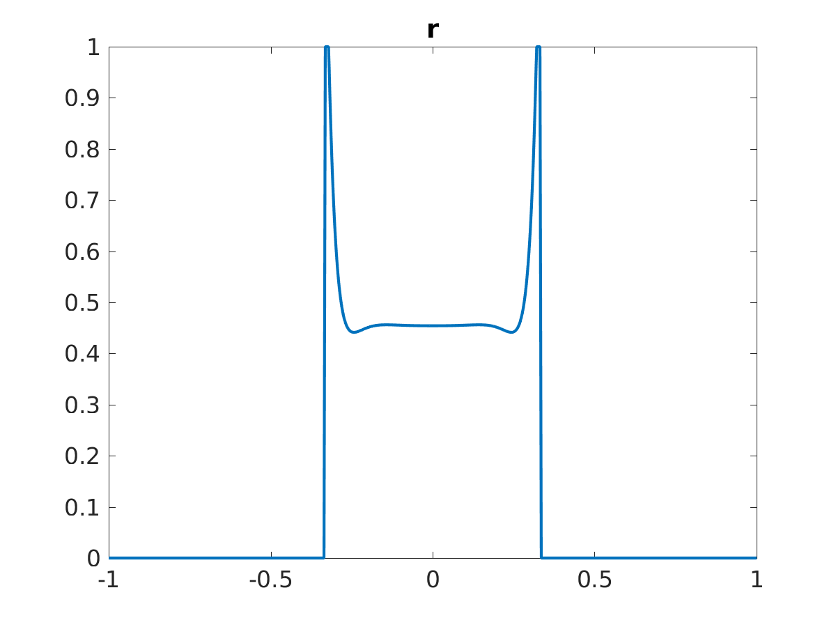
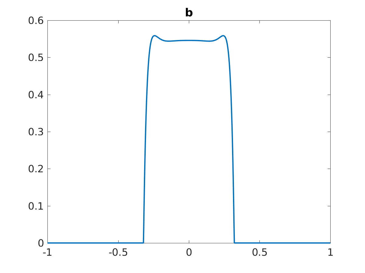
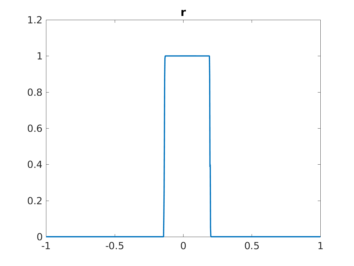
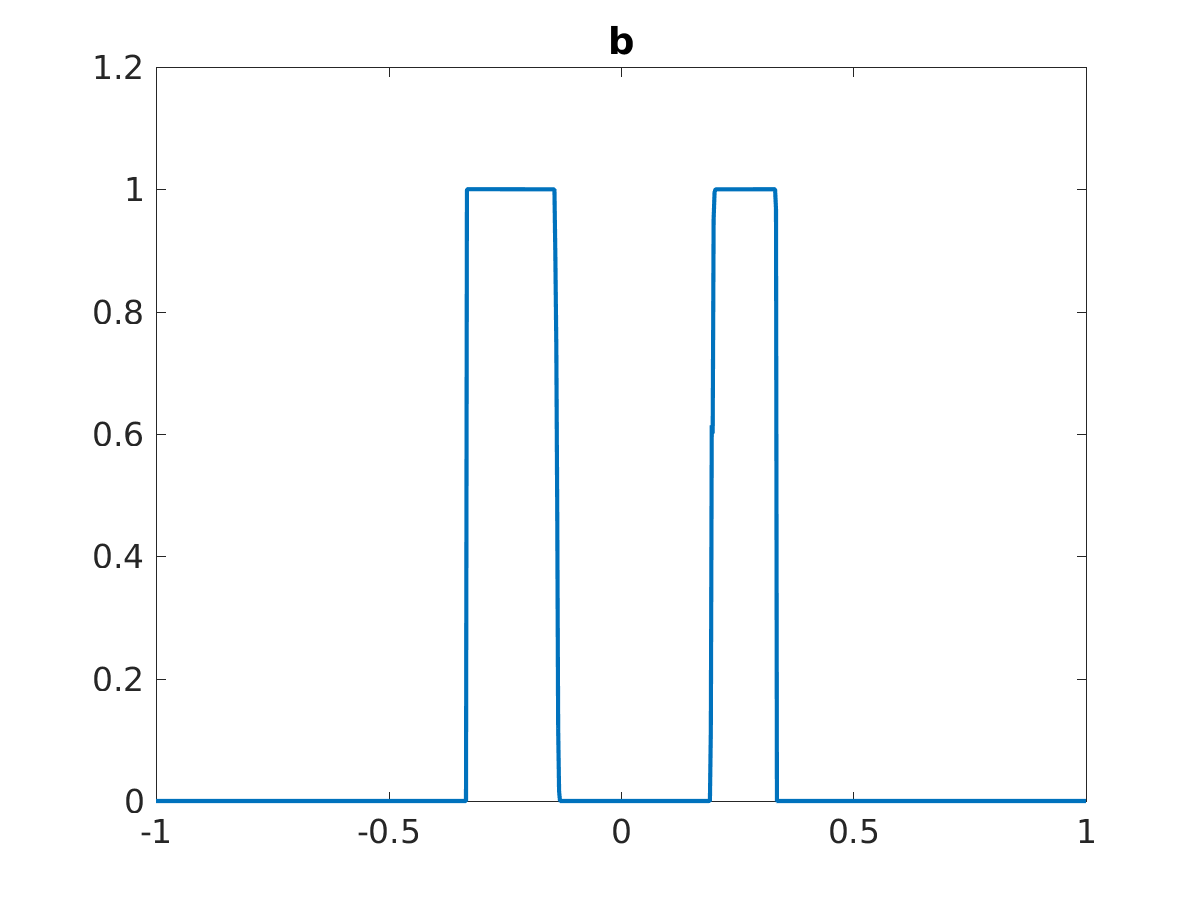
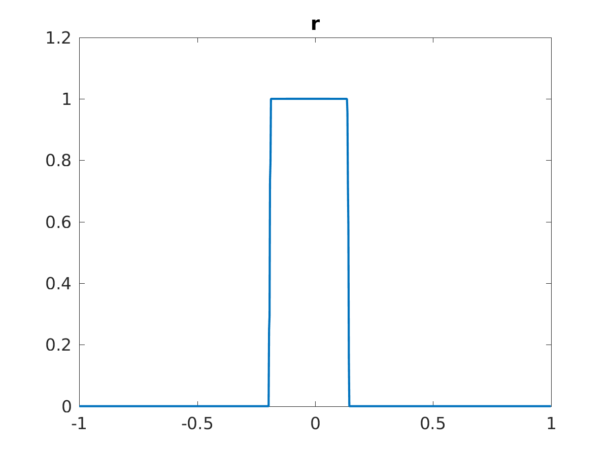
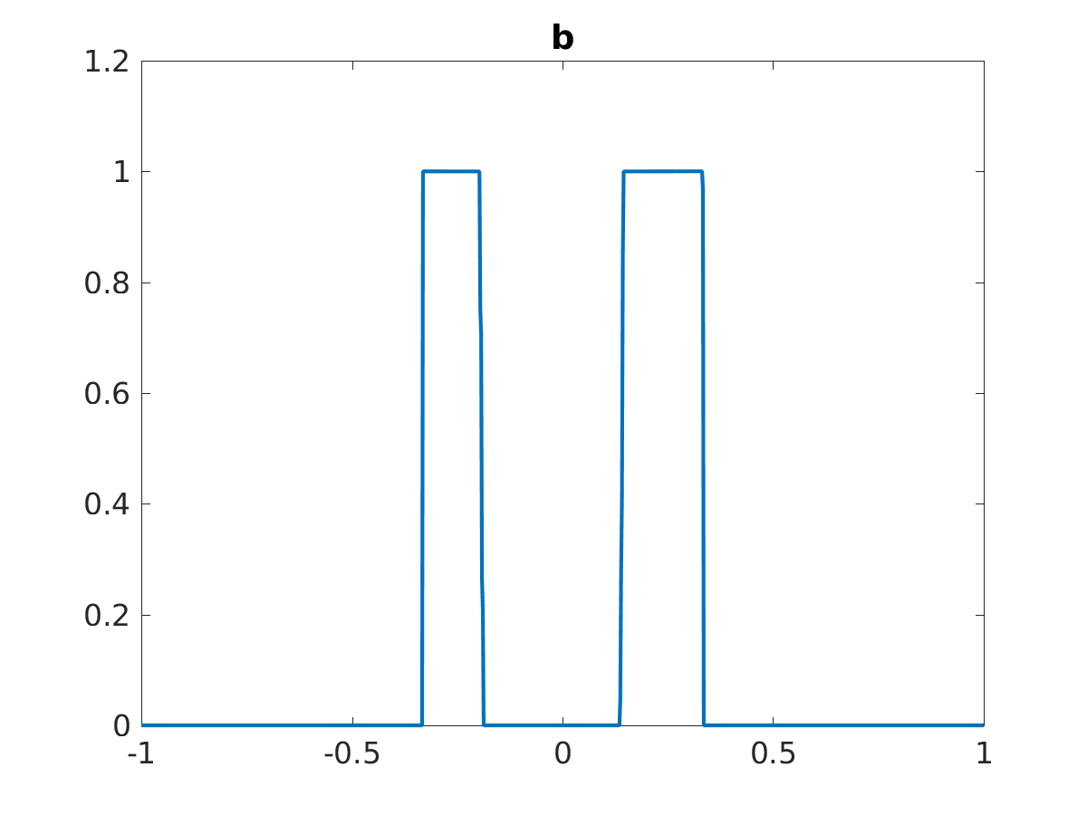
While all these examples are symmetric with respect to the origin, we can also obtain the asymmetric cases which appear for either and and or , see Figure 2. To break the symmetry, we multiplied the random initial data of by the positive function . For the case , left picture of Figure 2, we obtain one density surrounded by the other and taking the same initial conditions but values , we see that the support of the minimizers separate. This, for , corresponds to the situation where the smaller ball touches the boundary of the larger one, see again [33, Figure 2]. Finally, again for but the random initial data for multiplied by , we obtain a picture anti-symmetric to the first one, shown on the right. Since all initial guesses have the same mass, this also illustrates the non-uniqueness of minimizers.
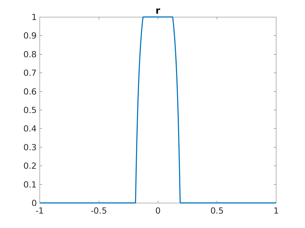
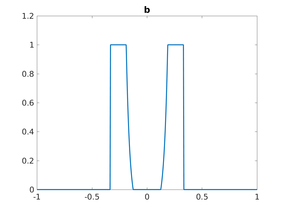
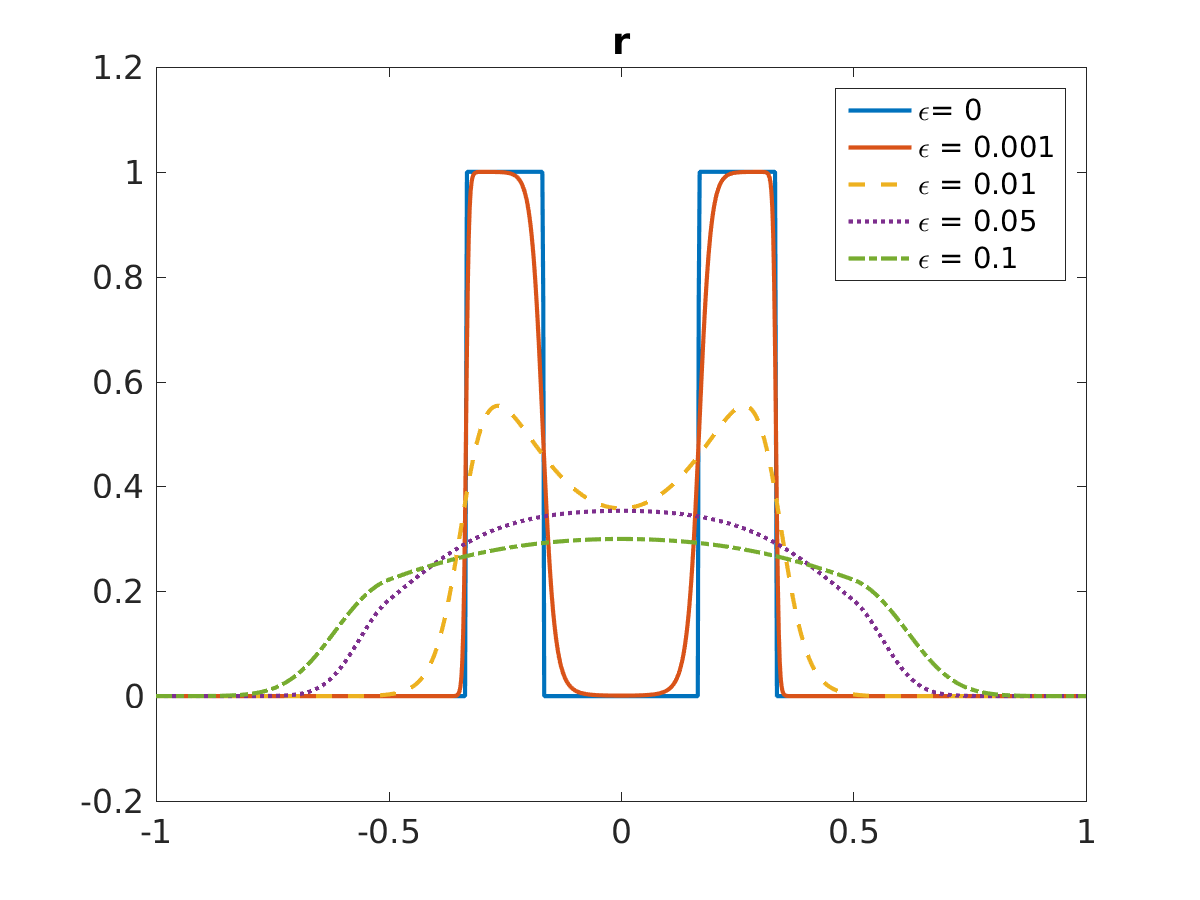
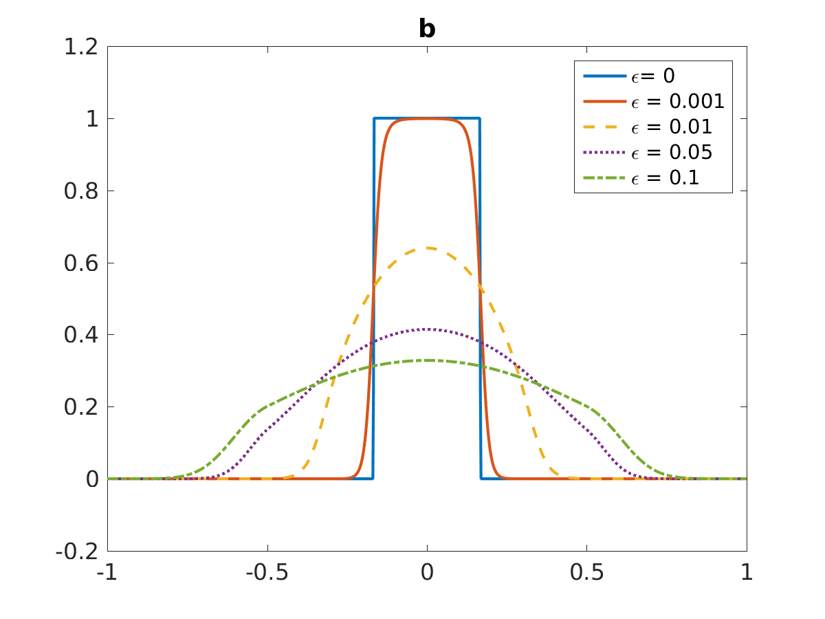
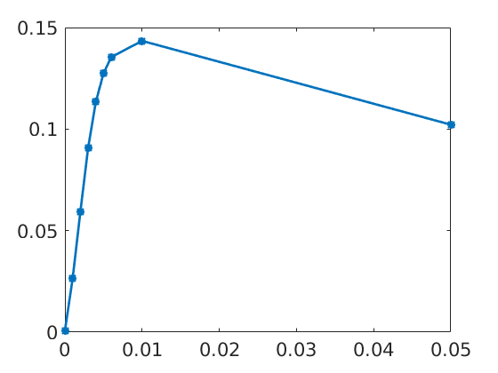
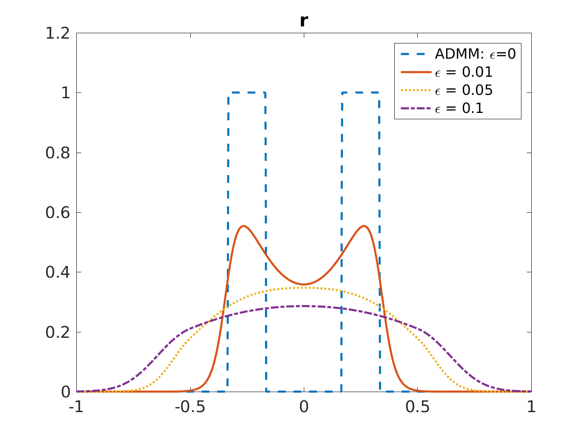
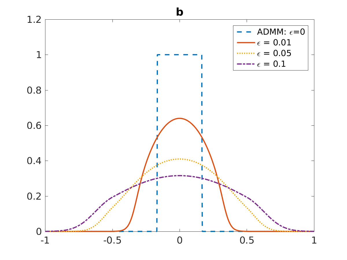
Next, we solve the minimization problem (3.1) for values . In Figure 3, we compare the corresponding minimizers to the case with the choice and . As expected, for small , the entropic part of the functional causes a smoothing of the minimizers. For larger , the energy becomes convex and we observe mixing without phase seperation as discussed in the introduction. This is also illustrated in Figure 3, where the integral of over is evaluated for different values of . For small values, a linear increase is observed while for large values, the overlap becomes very large and the integral cannot serve as an indicator for the overlap anymore.
3.2 Examples in Spatial Dimension Two
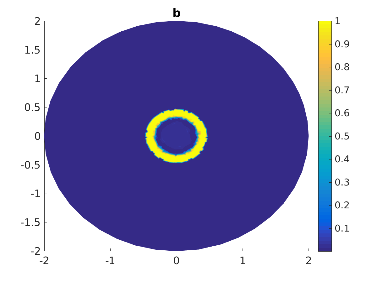
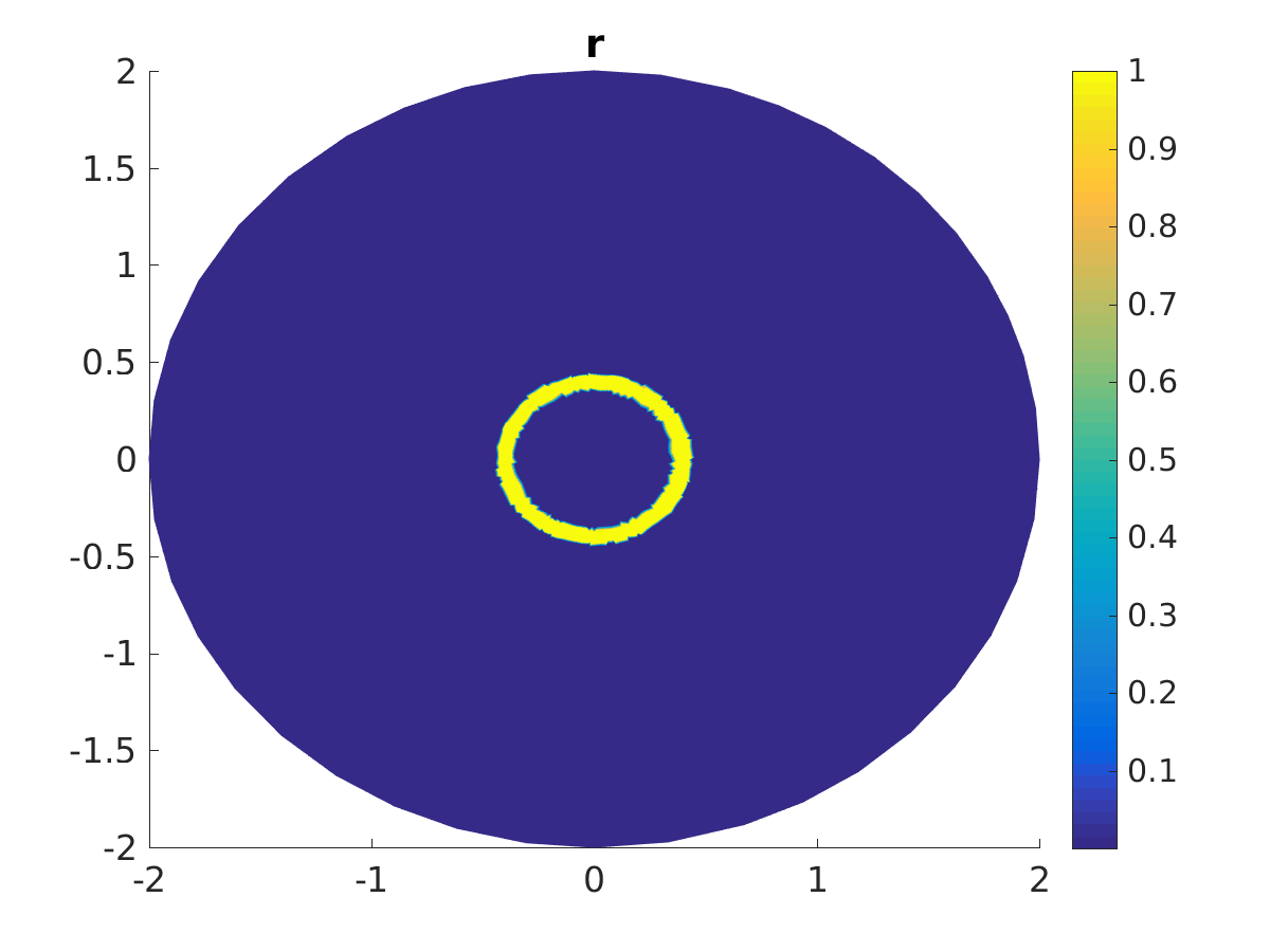
Next, we use our algorithm to solve the minimization problem in two spatial dimensions. Again, we first verify that we can reproduce the results of [33]. This is shown in Figure 4. We do not show the simulations for different since the results are very similar to the ones in one spatial dimension. The only difference is that we are not able to produce an asymmetric situation. For example, in Figure 4, right picture, we have the case with , and asymmetric initial data, yet we obtain a completely symmetric result. The same holds true for simulations with both and smaller than one.
,
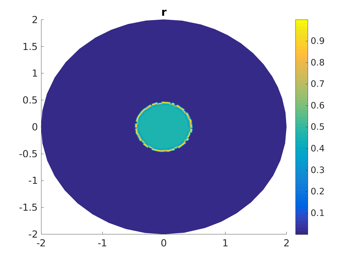
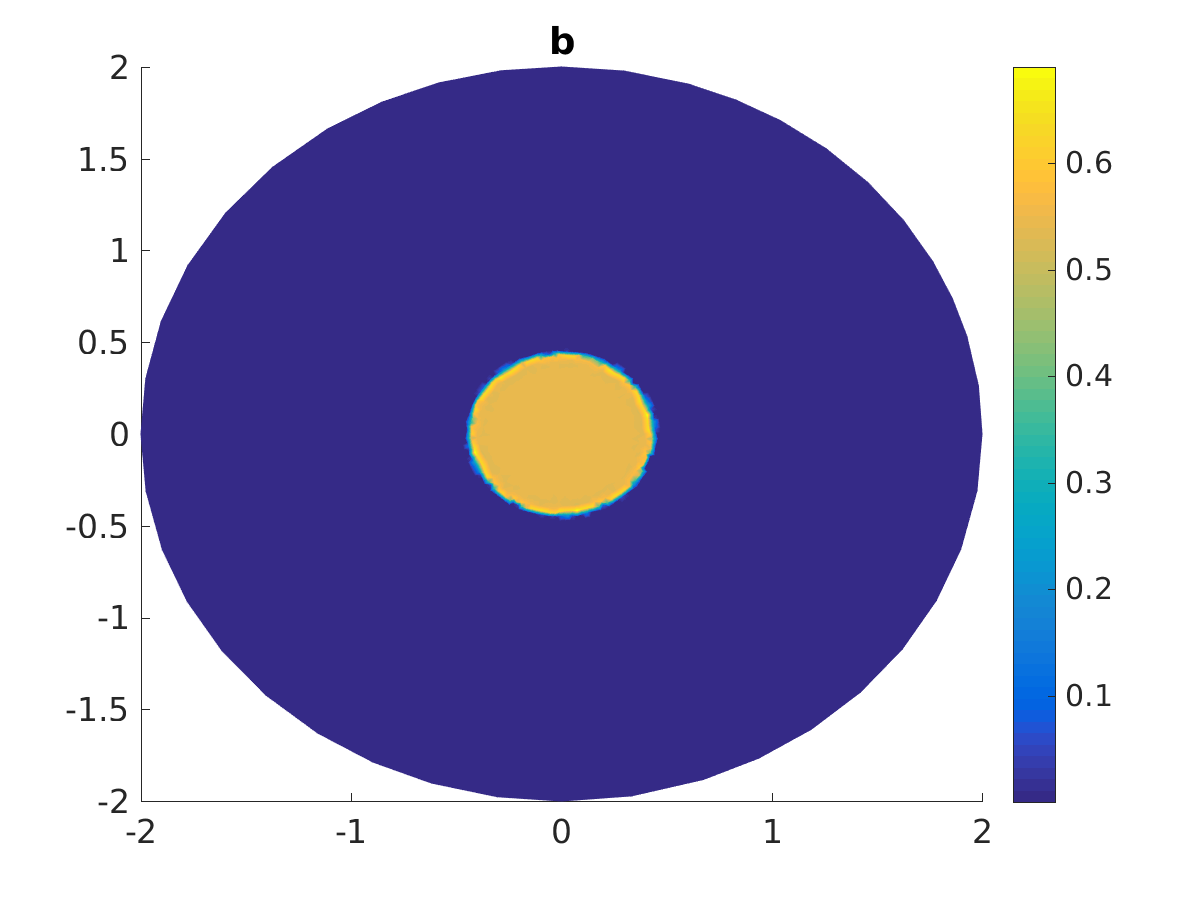
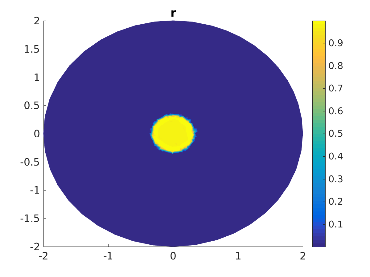
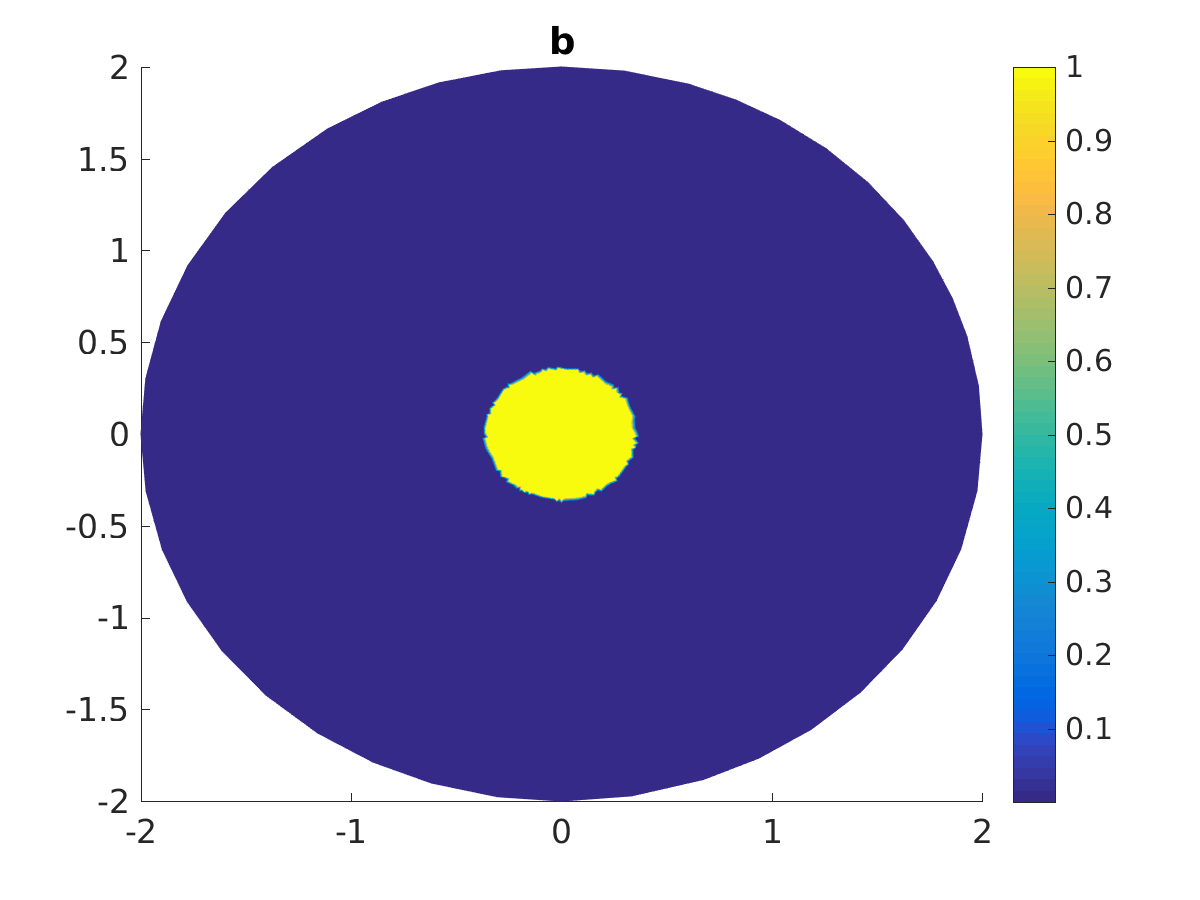
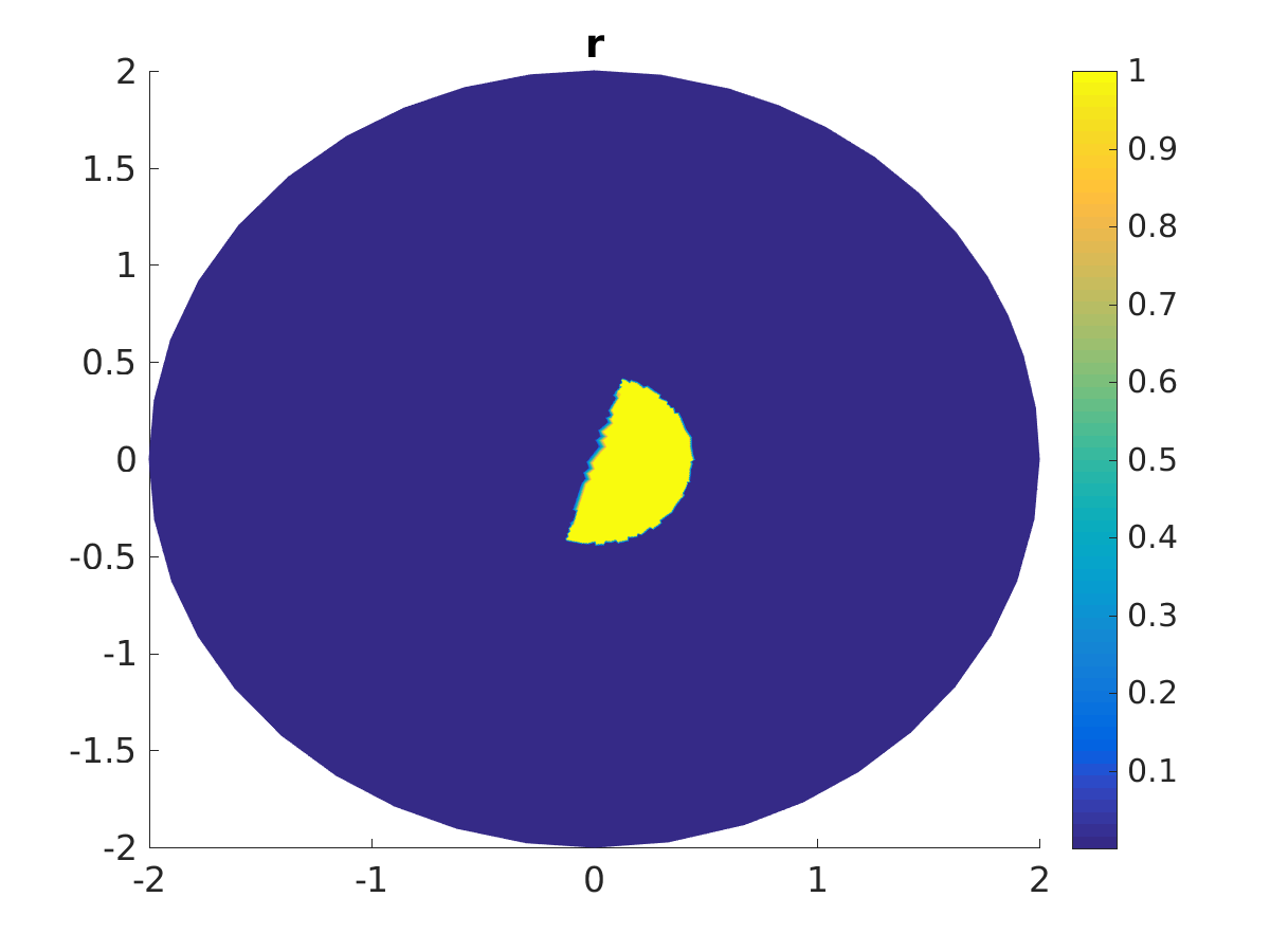
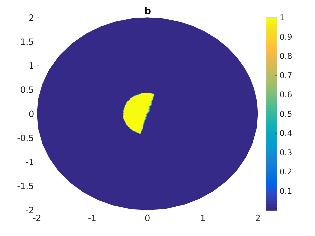
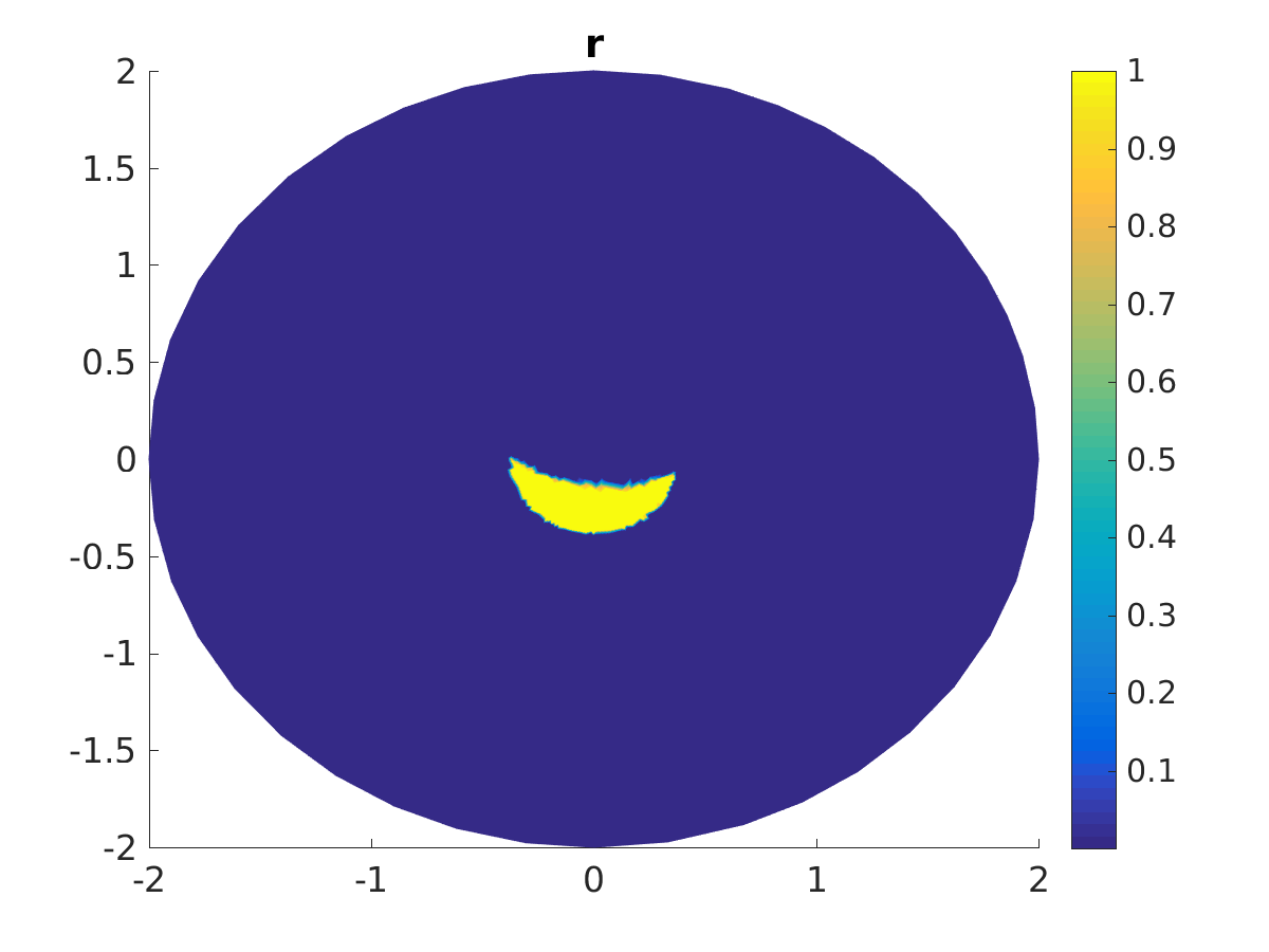
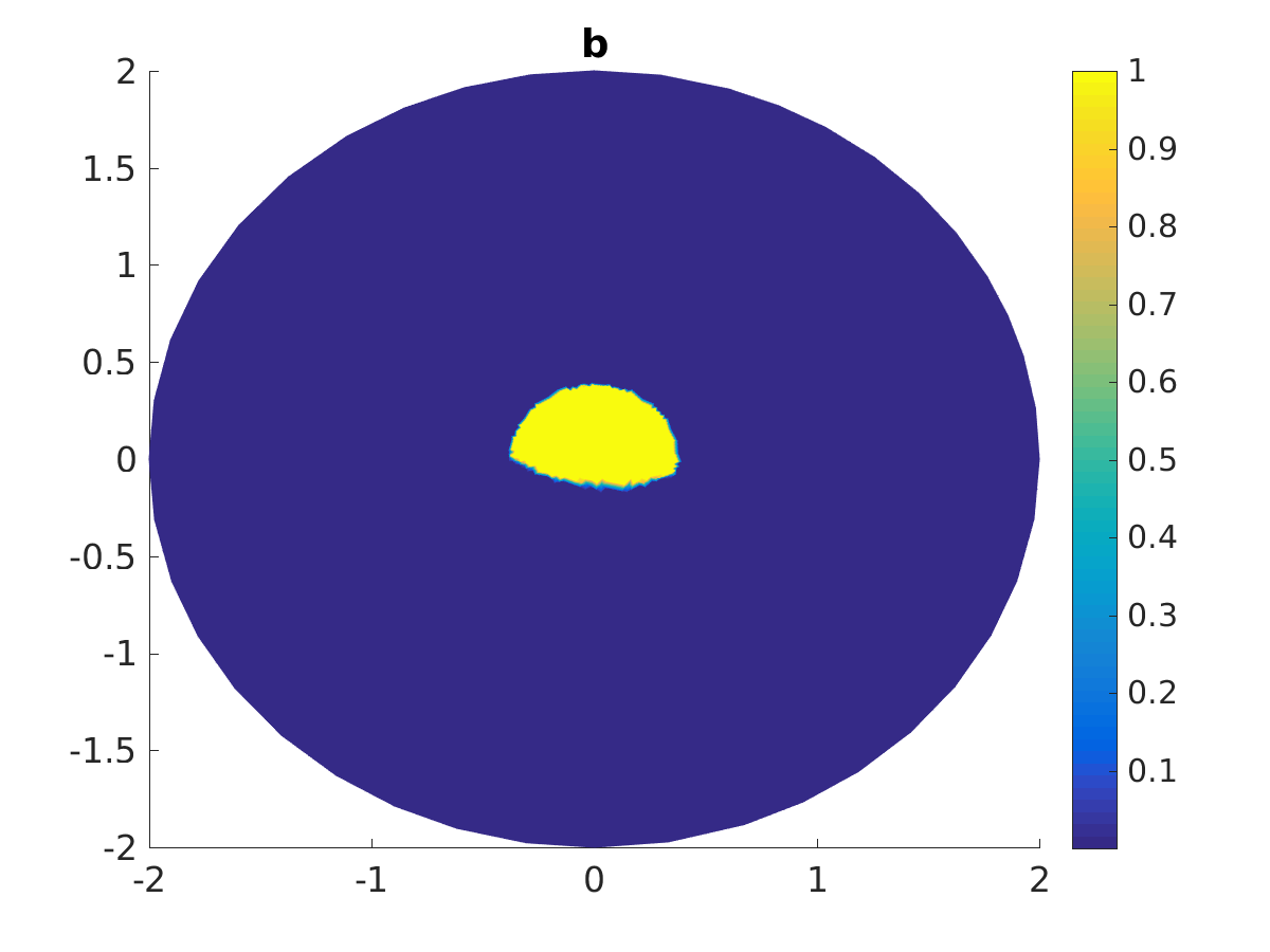
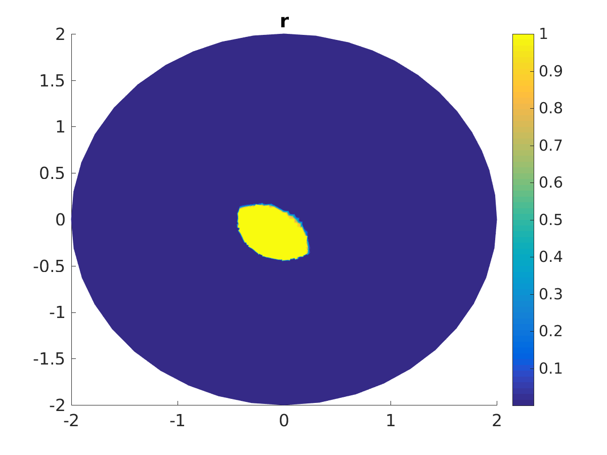
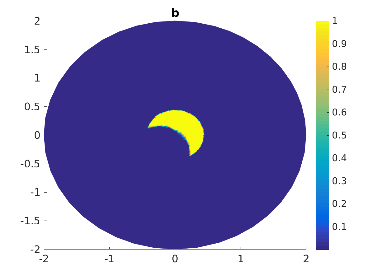
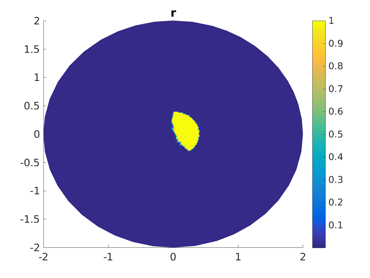
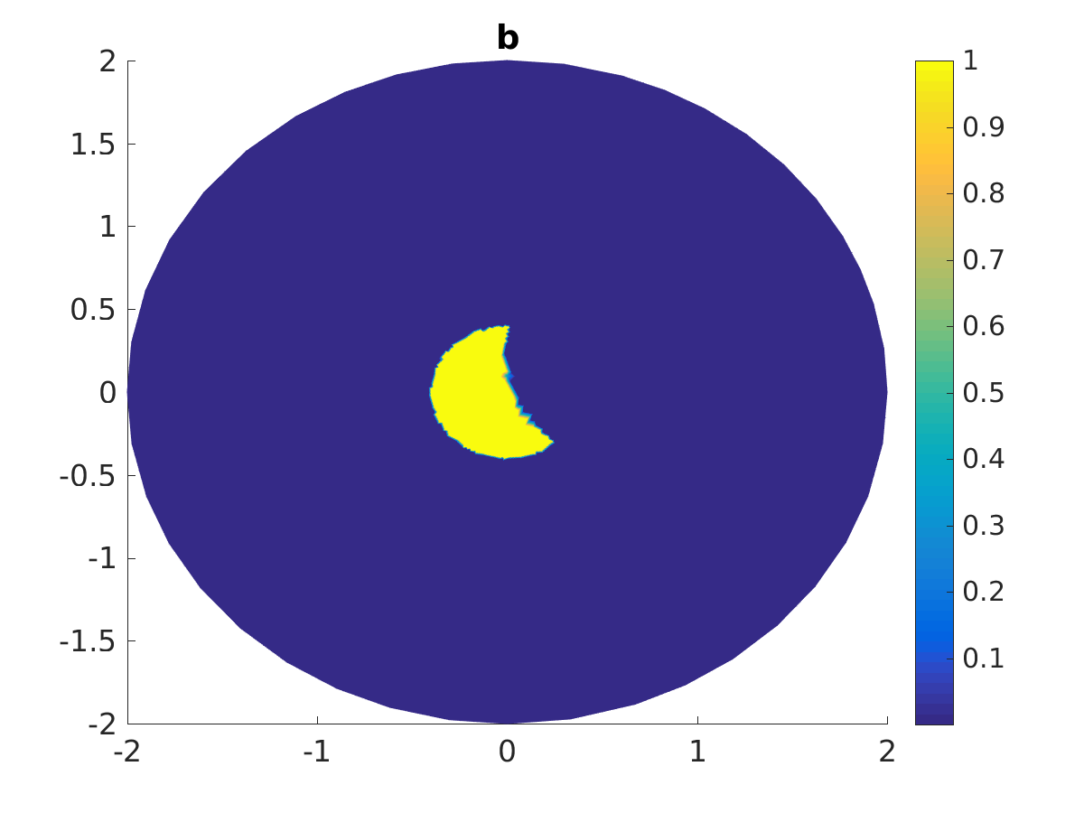
More interesting is again the case
In [33], an explicit characterization of minimizers in this case is only possible in one spatial dimension. It is, however, known that for , minimizers are characteristic functions of sets. By performing simulations, we confirm this results and are also able to characterize minimizers more precisely. In fact, for and , we see that the minimizers are two half balls, Figure 5 (left). Changing the mass of one species, we see that the interface between then changes from a straight line as in the previous case to a curved structure, Figure 5 (second from left). Varying also the constants and , as well as the masses, leads to similar results, see Figure 5 (third from left and right picture).
,
,
,
,
It is instructive to reinterpret the last results in view of (2.11). In the second column of Figure 4 we find the situation . Hence it is energetically favourable to avoid the interface between red and void, and put the largest interface between blue and void, which leads to an isoperimetric problem for the overall density. The partioning inside is simply obtained by a local isoperimetric problem for the red phase. The third column can be equally explained with the setting . The situation in Figure 5 is more subtle. Here and are expected to be lower than but the difference seems not large enough that a separation into two disjoint structures is favourable. On the other hand for large it is not favourable to create a ring as in Figure 4, but there is a local partitioning inside the ball leading to a smaller perimeter of the interface. We mention that numerical simulations with very large absolute values of the yield similar results, hence it is not clear whether the case of so large that it is favourable to create two separate structures for red and blue can be obtained as an asymptotic from our model.
4 Transient Model
As described in the introduction, minimizers of (1.6) are closely related to solutions of systems of nonlinear cross-diffusion partial differential equations [20]. In fact, introducing the nonlinear diagonal mobility tensor given by
we can introduce the following formal gradient flow with respect to
| (4.1) |
Inserting the definition (1.9) of , we obtain (1.3)-(1.4). This system is set on a domain and for . If is bounded, we impose the following no-flux boundary conditions
| (4.2) | ||||
on . This system is further supplemented by initial values
| (4.3) |
Using the functional , we introduce entropy variables, given as the first derivative with respect to and
| (4.4) | ||||
| (4.5) |
Inverting these relations yields
| (4.6) |
4.1 Existence of weak solutions
For further use we define the set
Global existence is guaranteed by the following theorem
Theorem 4.1.
Let , and . Consider the following partial differential equations on an open and bounded Lipschitz domain
| (4.7) | ||||
| (4.8) |
for satisfying (V1), for and as in definition (2.2). The system is equipped with initial conditions
with and no flux boundary conditions (4.2). Then there exists a weak solution in
such that
and furthermore and almost everywhere.
We remark that the proof without non-local interactions is given in [20, Theorem 4.1], yet using a different approximation technique. Here, we use a semi-discretization in time that has also been used in [23], but applied to a different, anisotropic system.
Proof.
Without loss of generality we choose in the proof and furthermore denote by a generic constant whose value can change from line to line. For different , some constants change yet the arguments remain the same. We prove the theorem in three steps: First we obtain an a priori bound based on the entropy dissipation, second we apply a time discretization and use a fixed point argument to ensure existence of weak solutions for every time step. Finally, we finish the proof passing to continuous time.
First step: Entropy inequality We calculate the dissipation of the diffusive part of the energy functional
Using the gradient of the entropy variables (4.4)–(4.5)
we obtain
| (4.9) | ||||
By the definition of the entropy variables (4.4)–(4.5) we see that . Therefore take finite values almost everywhere and we conclude that , see also [49]. Since as defined in 2.2 and is bounded, we can apply Young’s inequality for convolutions
and the analogue for Now, rewriting (analogously for ) and using Young’s inequality allows us to absorb terms and we obtain
| (4.10) |
where in the last step we used . The positive constant depends on the interaction kernel and on the constants only. In particular, it only depends on the size of the domain via the -Norms of and . Expanding the terms containing and and integrating in time we finally obtain
Now we can use the Young’s inequality weighted with together with the fact that is bounded in
| . | |||
Summarizing we find
| (4.11) |
Second step: Time discretization We continue by rewriting the system using again the definition of the entropy variables (4.4)–(4.5). We obtain
Next we discretize the system in time using the Euler implicit scheme. We split the time interval as
with Furthermore, we add an additional regularization term. The system then becomes
| (4.16) | ||||
| (4.19) |
We consider the weak formulation of the problem (4.16) for all
| (4.28) | ||||
| (4.35) |
where we introduced
| (4.36) |
and
| (4.37) |
Note that the matrix is positive semi-definite, because and We furthermore abbreviated the regularization term as
| (4.38) |
To solve the nonlinear equation (4.28) for , we first linearize it by replacing the terms and by and , respectively for given and . To treat this linear problem, we introduce the bilinear form
given by
| (4.47) |
and the linear form
Thus, (4.28) is equivalent to
| (4.48) |
Writing out the definitions of the matrices, it is straight forward to see that is bounded
The regularization term ensures the coerciveness of
The boundedness of as a linear functional is a consequence of Young’s inequality for convolutions and the regularity of . We conclude existence of unique solutions since all assumptions of the Lax-Milgram lemma, [38, Sec. 6.21., Thm 1], are satisfied. This allows us to define a fixed point operator
with being the unique solution to (4.48). We aim to apply Leray-Schauder’s fixed point theorem as stated in [42, Thm 11.3]. We know that is bounded in because is assumed to be bounded
and the analogue for the second component
It remains to establish compactness of . Consider a sequence that converges to strongly in . Since , the regularization term ensures that are uniformly bounded in and thus there exists subsequences (which we don’t relabel) such that their gradients converge weakly in . Since the entries of are uniformly bounded in , we also have strong convergence of to in . This, together with a standard approximation of the test functions in allows us to pass to the limit and conclude the continuity of . For the linear form , continuity, now with respect to is once more a consequence of Young’s inequality for convolutions. Finally, the fact that the mapping (4.6) is differentiable and thus Lipschitz continuous, we conclude the continuity of the whole operator . Together with the compactness of the embedding , Schauder’s fixed point theorem can be applied.
That means we have established existence of weak solutions for every iteration step.
Third step: Limit Now we extend the result to continuous time, i.e. we consider the limit . We want to use the convexity of the entropy which together with its differentiability implies that
Now we discretize time and choose and Using the definition of the entropy variables given in (4.4)-(4.5) yields
We insert this inequality into the weak formulation (4.28) of our problem for , we find
Solving this recursion w.r.t. gives
As a next step we use a piecewise constant interpolation, i.e. for and we define
Furthermore let be the shift operator such that for
Then solves the following equation
| (4.57) | ||||
| (4.64) |
Now, using again Young’s inequality and reiterating the same steps as performed when deriving (4.1) from (4.9), the above inequality becomes
| (4.69) |
In order to pass to the limit and to show the convergence and we need the following two lemmas.
Lemma 4.2.
The following estimates hold for a constant and
| (4.70) | ||||
| (4.71) | ||||
| (4.72) |
Lemma 4.3.
The discrete time derivatives of and are uniformly bounded
| (4.73) |
The first lemma is a direct consequence of the discrete in time entropy inequality (4.1), see [57, 23] for details. The second results from using the estimates of the first one in the weak formulation (4.28). Now we apply a special version of the Aubins-Lions lemma specifically designed for piecewise constant interpolations, cf. [35, Theorem 1]. Using the Gelfand triple this theorem implies that (4.73) together with the boundedness of in is sufficient to obtain a strongly converging subsequence such that (without relabeling)
This implies
But since the space embeds continuously in the function must also converge strongly to in . Note that (4.72) immediately implies
Finally, since are uniformly bounded in , we know that there exist subsequences such that
| (4.74) |
In order to be able to pass to the limit in (4.28), we rewrite
The first term on the right hand side can be dealt with by further expanding the term , the fact that converges strongly, using the bounds (4.70) and the fact (4.74). For the second term, one has to prove strong convergence of which can be done either by using the Kolmogorov-Riesz theorem, see [20] or again a generalized Aubins-Lions lemma, see [64]. Note that this strong convergence also allows us to identify the corresponding, weakly converging gradient. ∎
As a next step, we extend the previous result to the case . The crucial ingredient will be the entropy inequality, which also holds on the whole space. We have
Theorem 4.4.
Proof.
The proof is based on the same a priori estimates as in the bounded domain case and thus we only sketch the additional arguments. Indeed, the main ingredient is the entropy inequality, (4.1) which, due to the uniform -bounds on and also holds on . This in particular implies the second moment bound on and which in turn yields the compactness of the embedding from to . Indeed, taking a sequence we have, for some and fixed that
Using the -bound on and , we can estimate the second term on the right hand side and obtain
Taking the , we see that the first term on the right hand side vanishes due to the compactness of for fixed . Taking, in a second step the limit yields the assertion.
Now we generate a sequence of approximate solutions and by solving the problem
| (4.83) | ||||
| (4.86) |
where we use restrictions of and to as initital conditions. Due to the two ingredients, namely entropy inequality and compactness, we can pass to the limit exactly the same way as we did for time discretization in the proof of the previous theorem. The bounds of the right hand side of the weak formulation (4.83), again together with the second moment bound, then also yield the -bounds for the time derivatives. ∎
For , we have the following regularity result for which may serve as a first step in proving uniqueness of solutions via a fixed point argument in that case.
Proposition 4.5 (Regularity of for ).
Proof.
For , we can add equations (4.7) and (4.8) to obtain an equation for given as
| (4.87) |
with
and initial datum
Using the regularity of and as well as the properties of , we can estimate as follows
Since the constant on the right hand side does not depend on we can take the supremum over all and conclude that . Thus applying the theory for linear parabolic equation, see e.g. [51, Chapter VII], yields the assertion. ∎
Remark 4.6 (Minimizers as stationary solutions).
5 Numerical Simulations
This Section deals with a numerical algorithm to solve the the PDE system (4.7)–(4.8) supplemented with no flux boundary conditions. We use the same P finite element method as described in (3). To discretize in time, we use the following implicit-explicit scheme: Given inital values and denoting the current iterates by (with ), we obtain new iterates by solving the linear system
with time step size given. Again, we use MATLAB for the implementation, both in one and two spatial dimensions.
5.1 Examples in one spatial dimensions
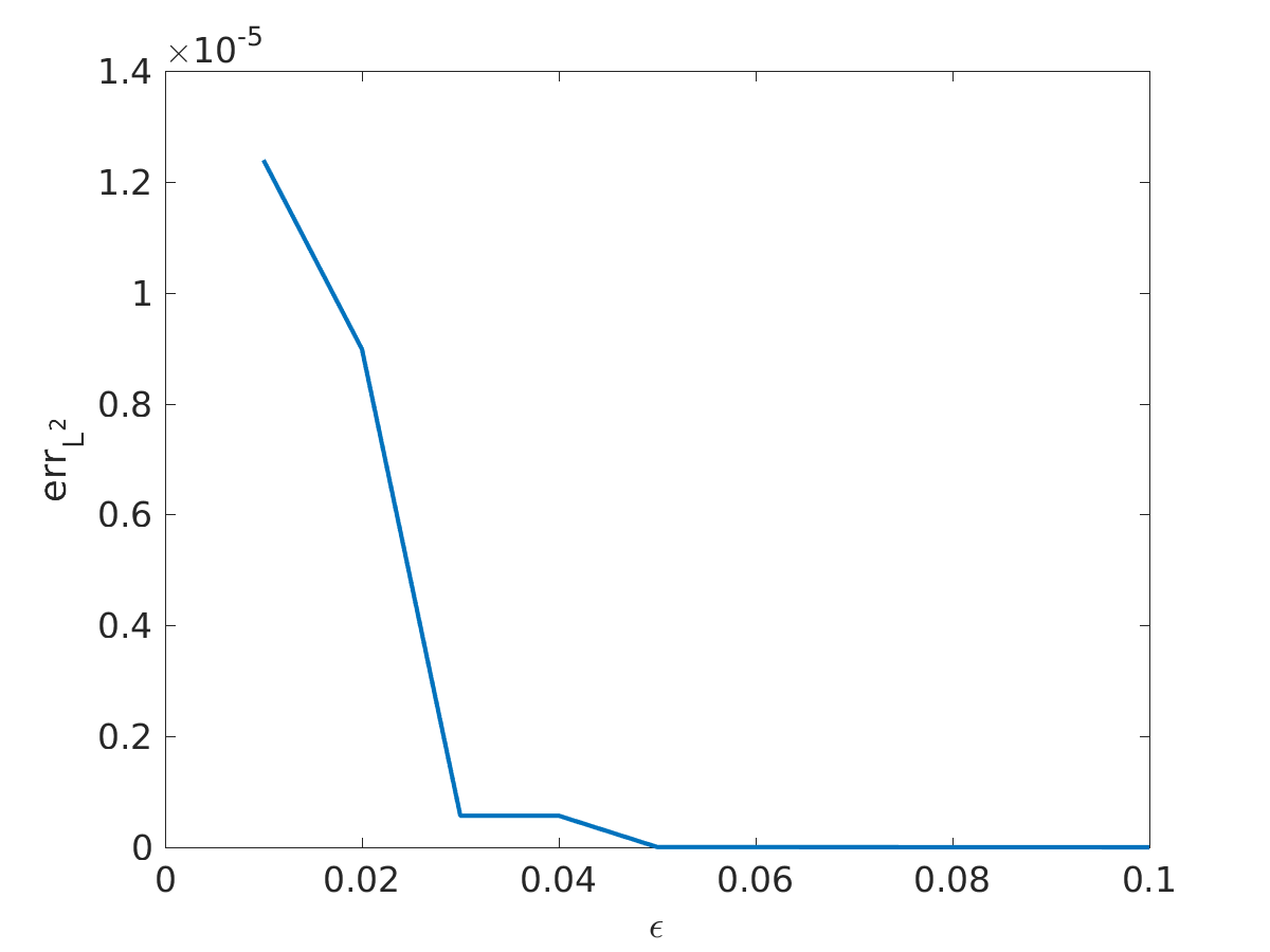
For all one-dimensional examples, we use the same potential as in Section 3, defined in (3.28) Furthermore, to decide when we reached a stationary state, we consider the relative -error between two iterates, i.e
and stop the iteration as soon as . We start by comparing the solutions for different values of to that of the ADMM scheme. As initial values we take
| (5.1) |
where is the following approximation of the Heaviside function
| (5.2) |
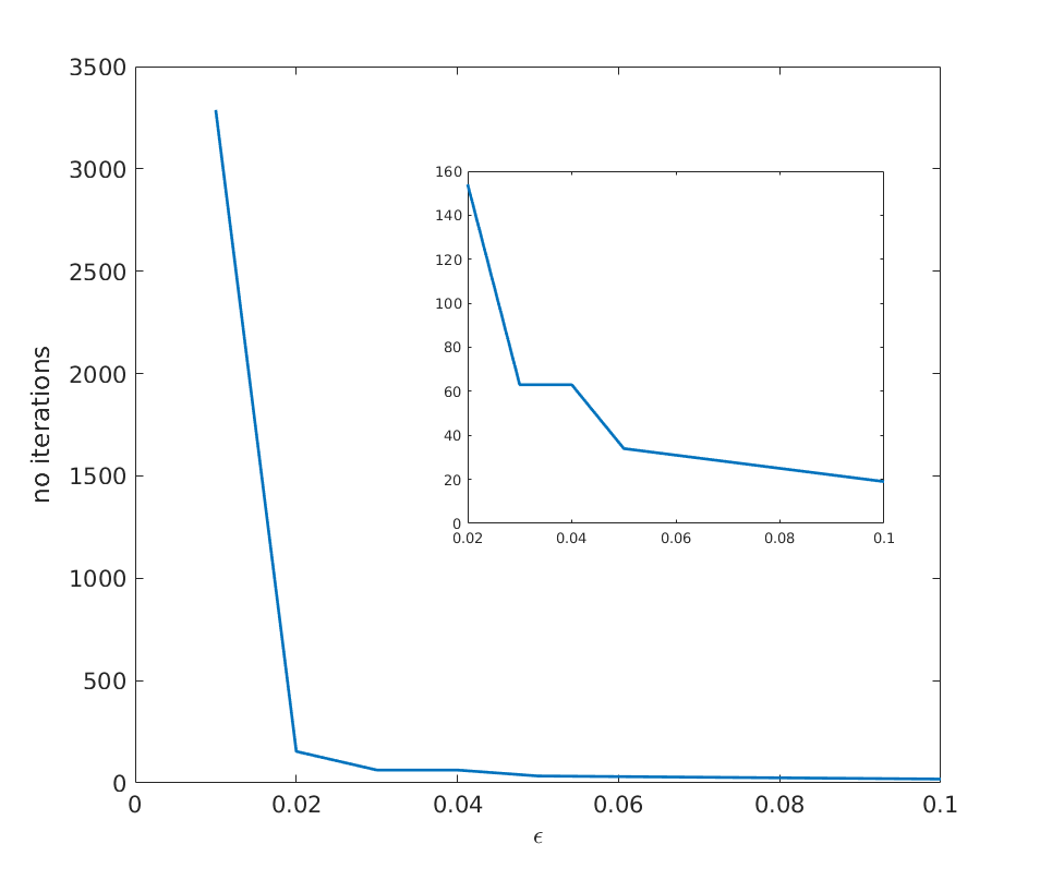
The results are visualized in Figure 6 (left). In the top right picture the number of iterations until the error criterion is met are shown. On the bottom right, we plot, for a fixed time (and thus a fixed number of iterations), the relative error that is achieved for different values of . As expected, both plots confirm that the dynamics become slower as becomes smaller - see the discussion about the relationship to systems of Cahn-Hilliards equations in the introduction.
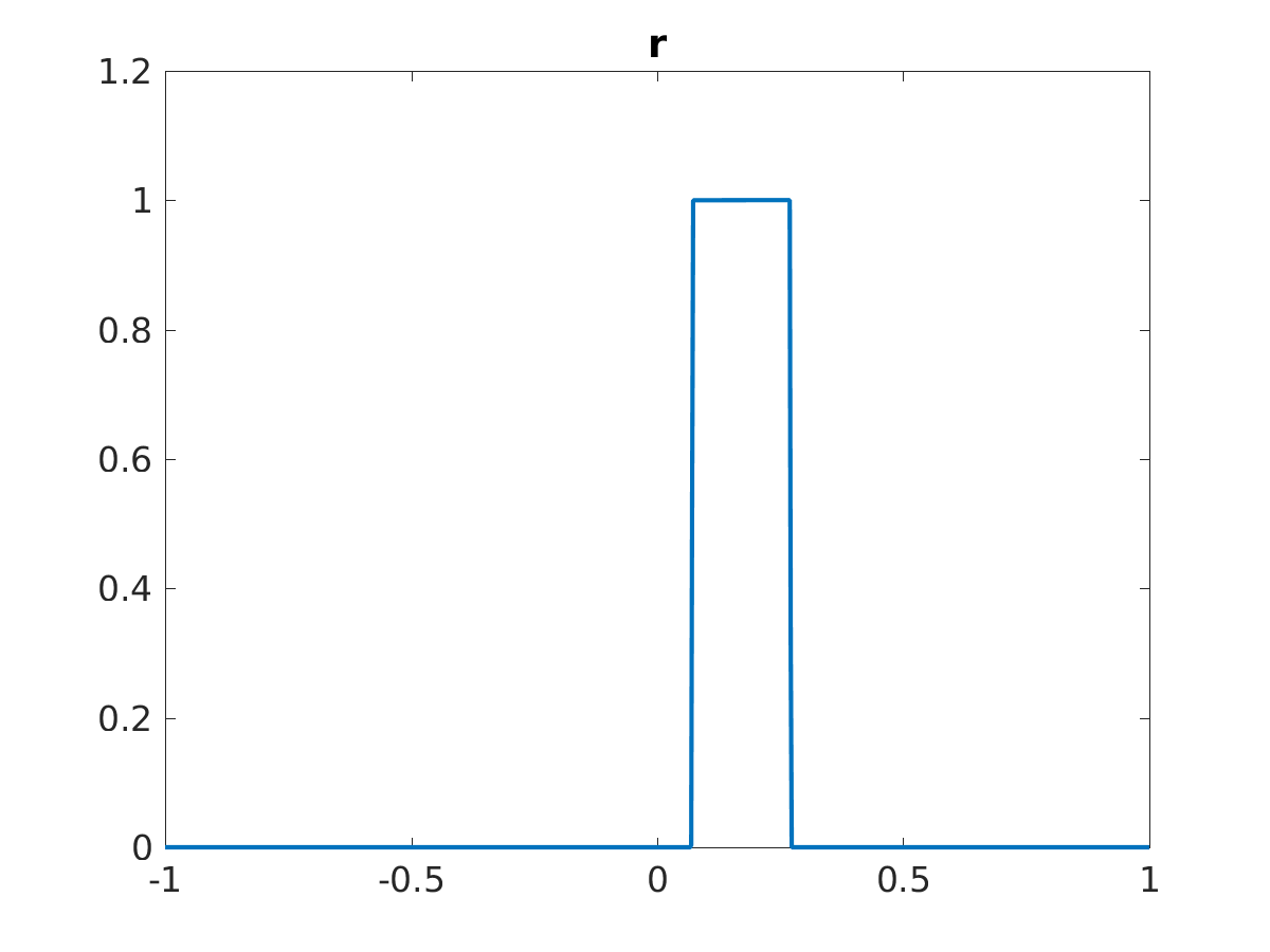
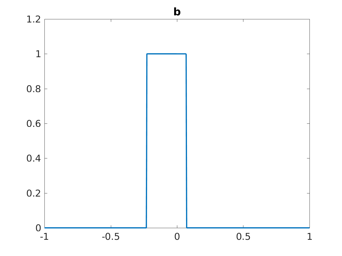
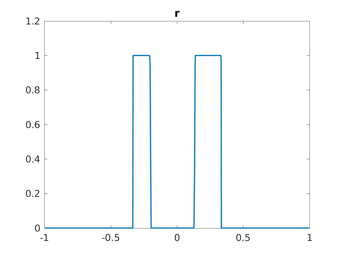
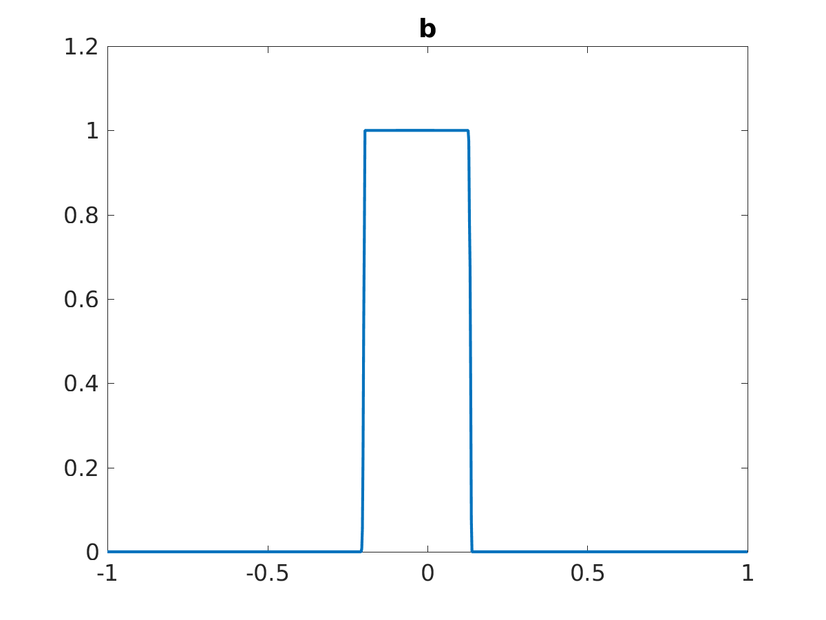
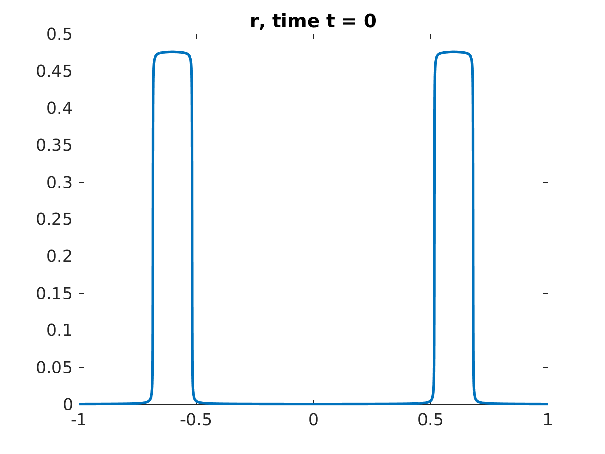
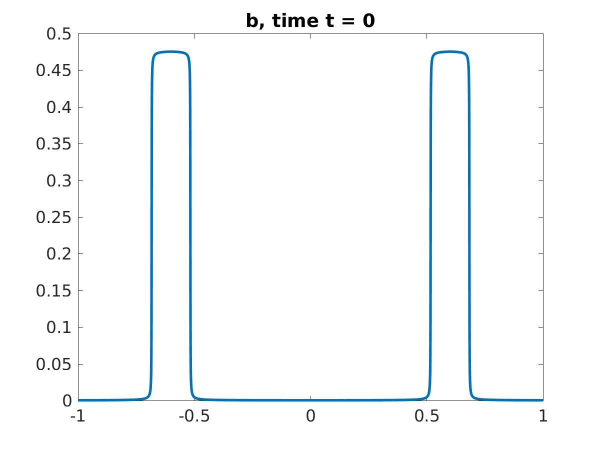
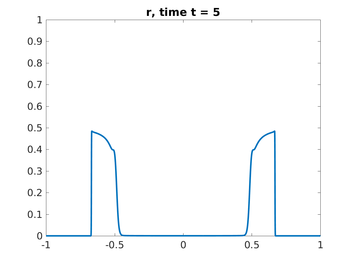
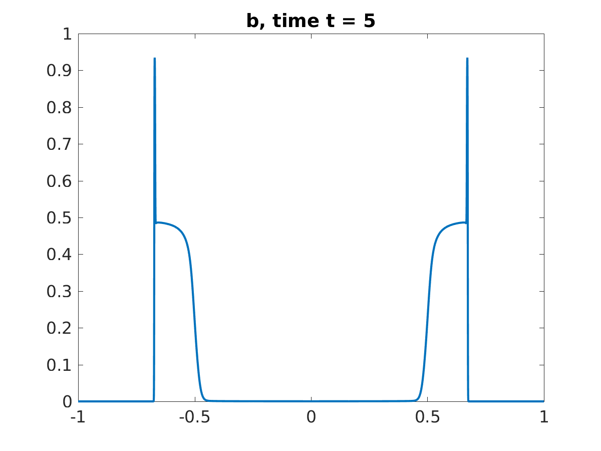
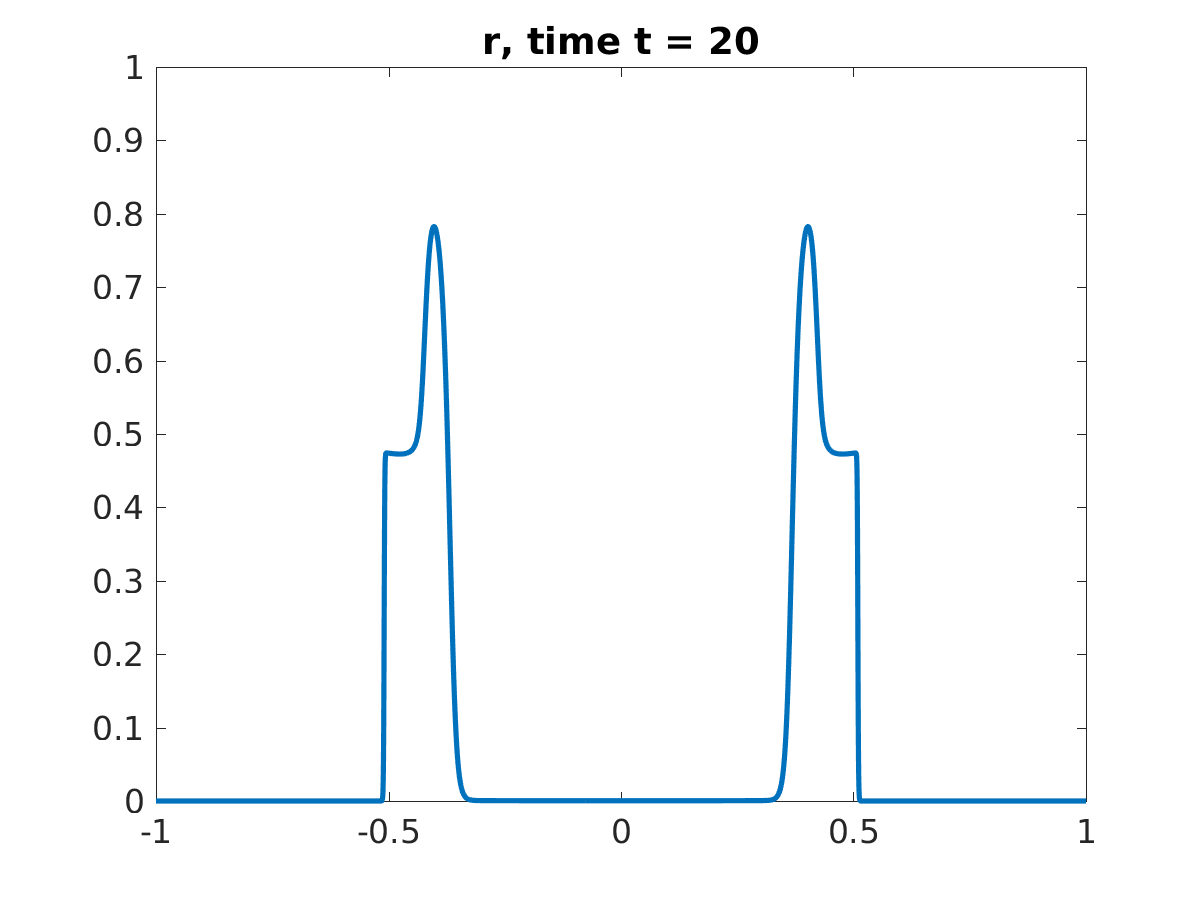
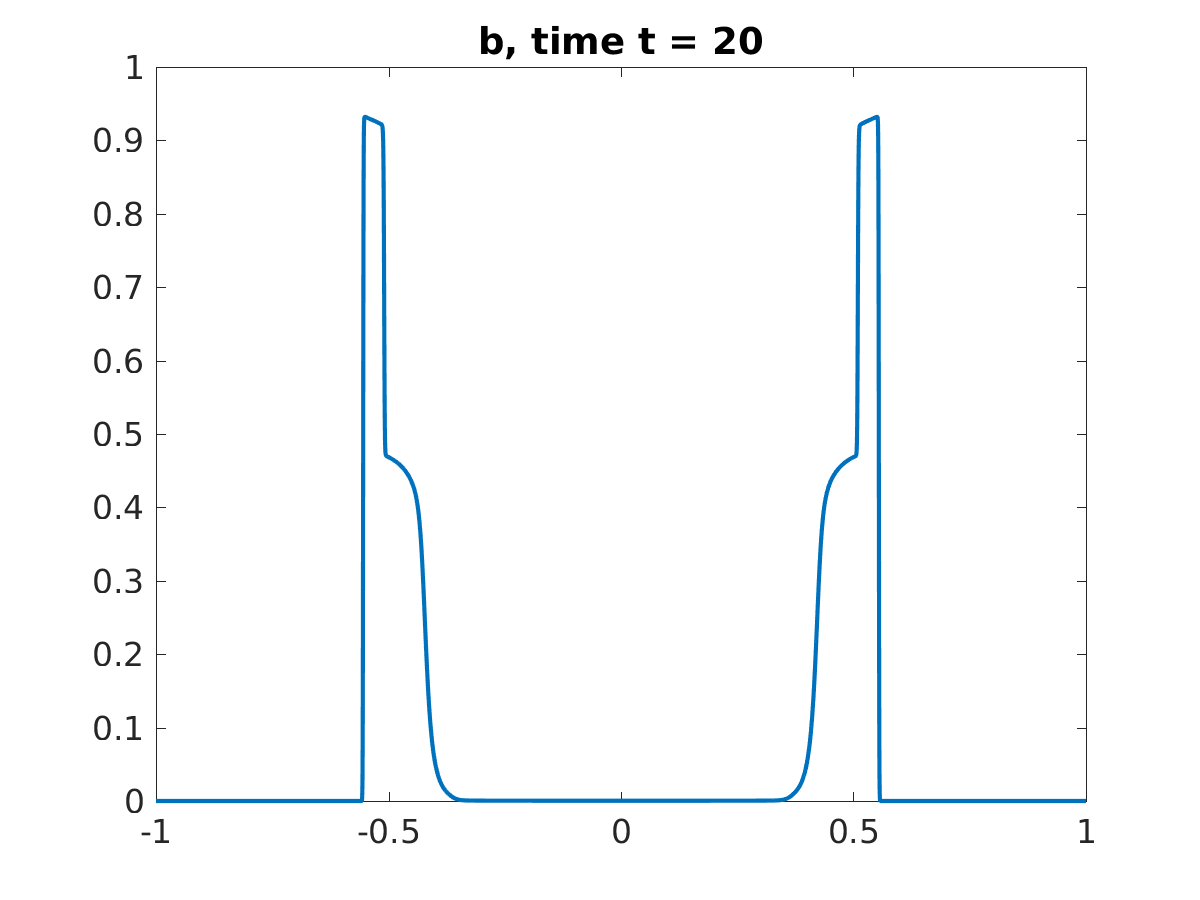
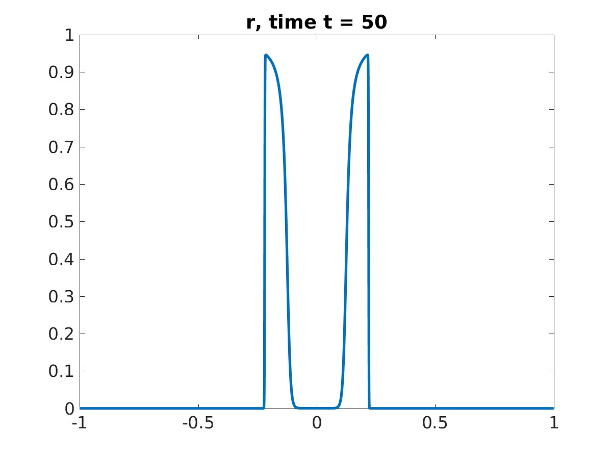
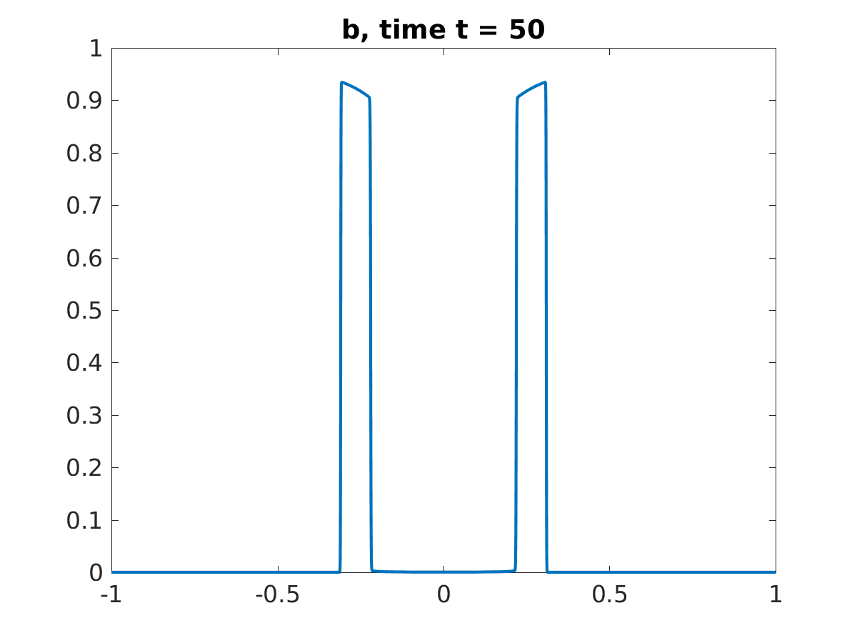
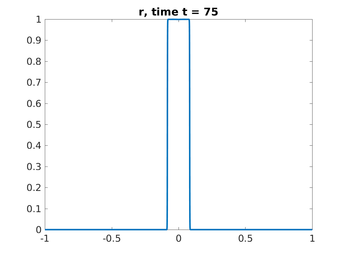
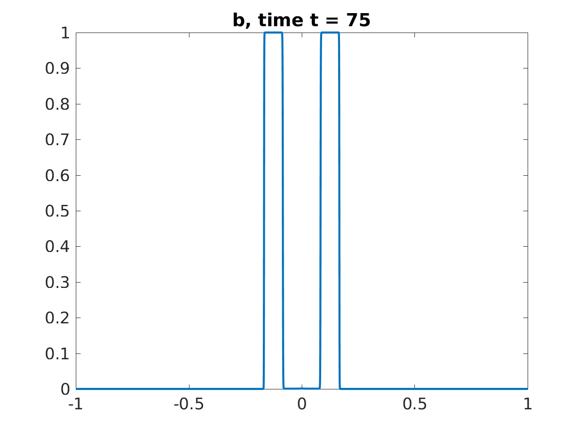
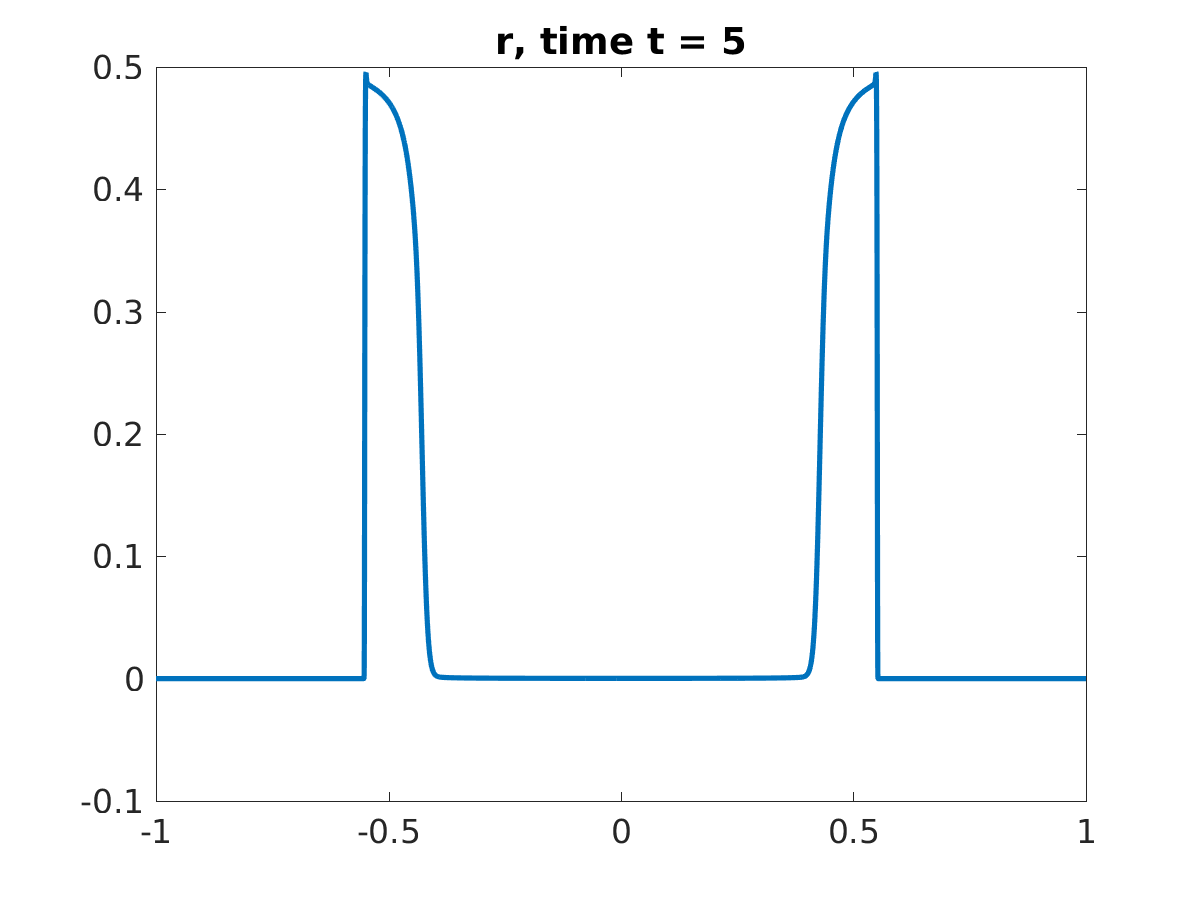
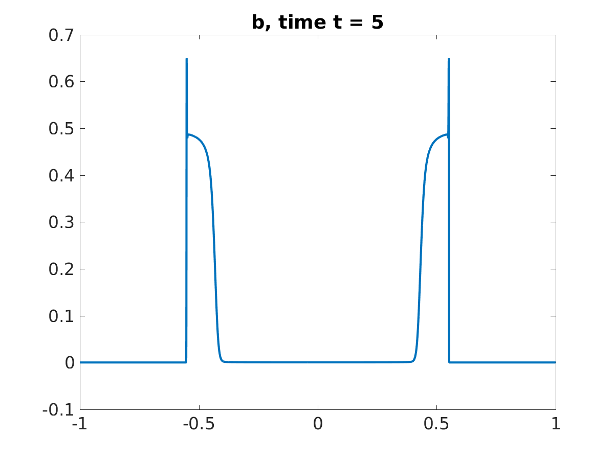
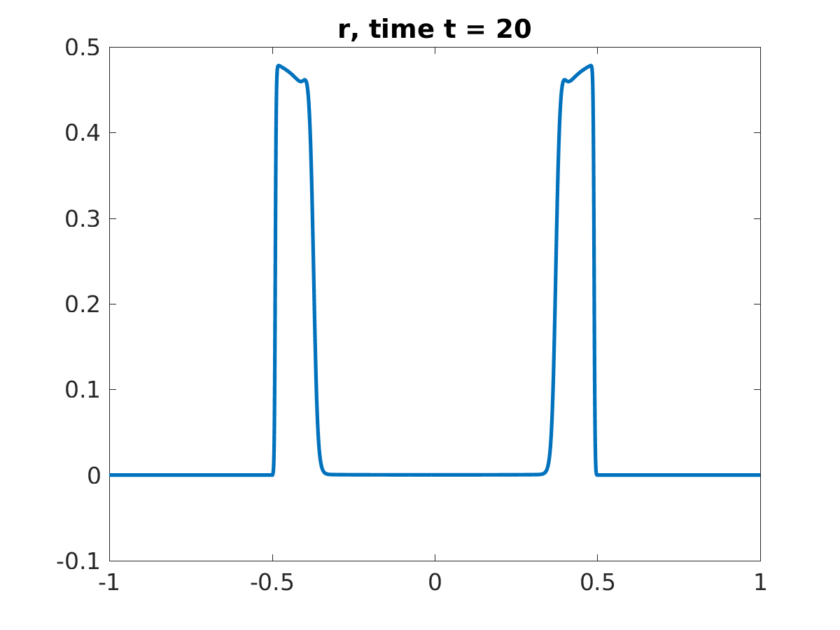
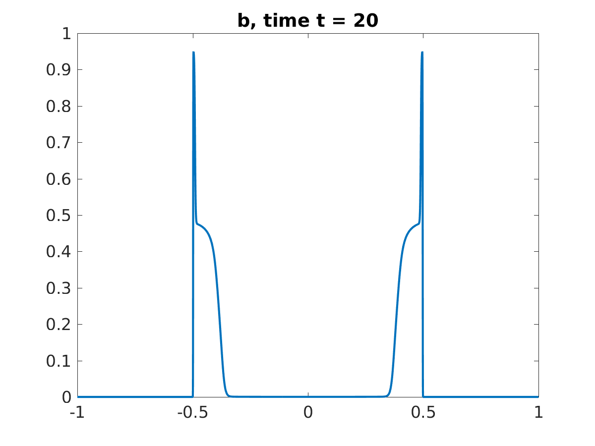
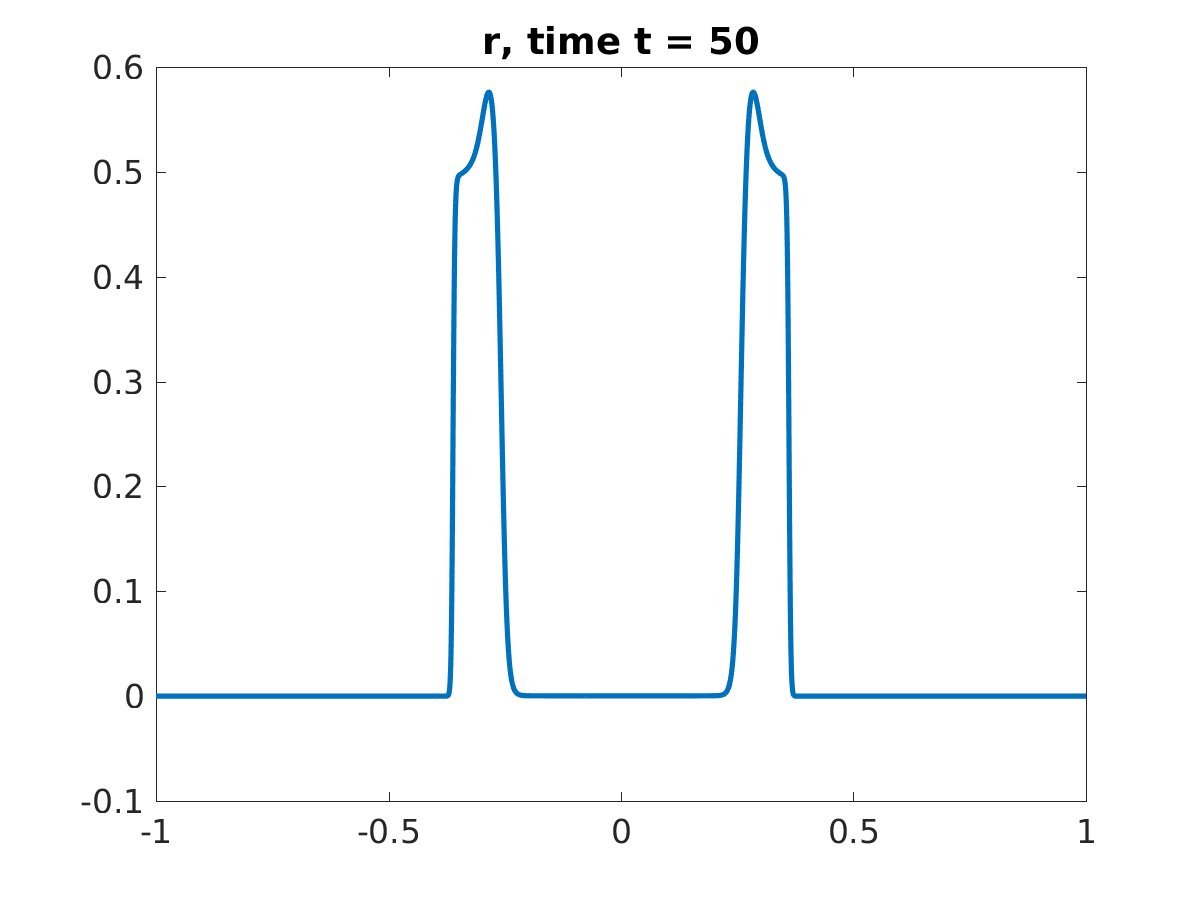
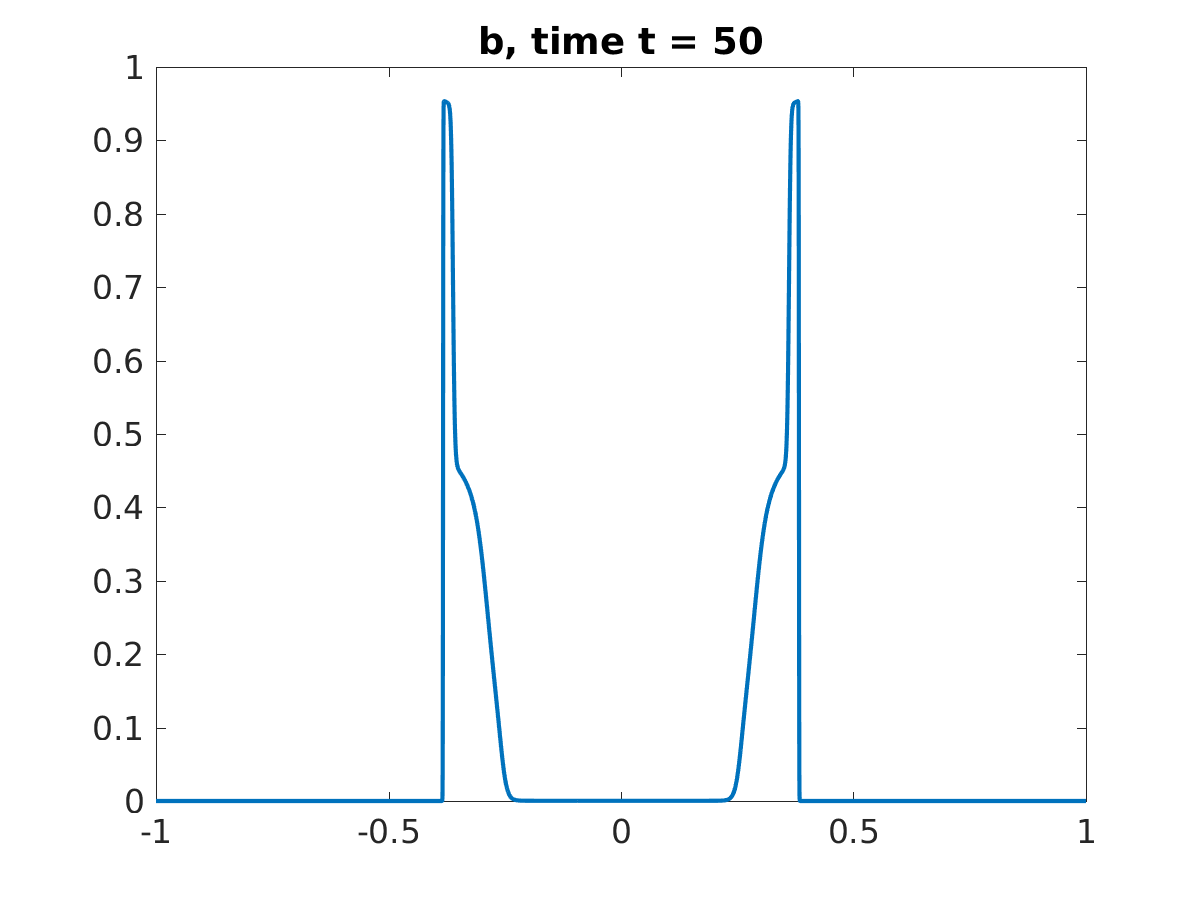
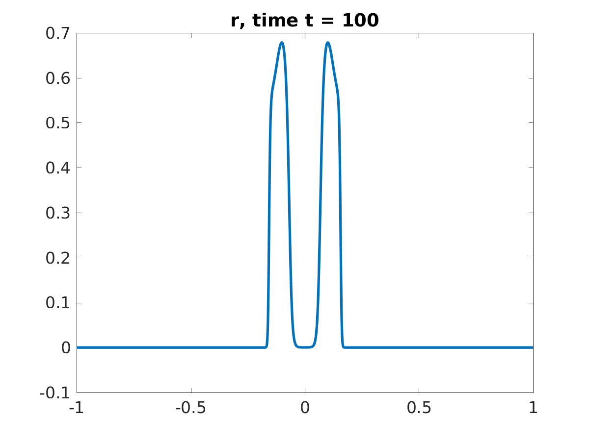
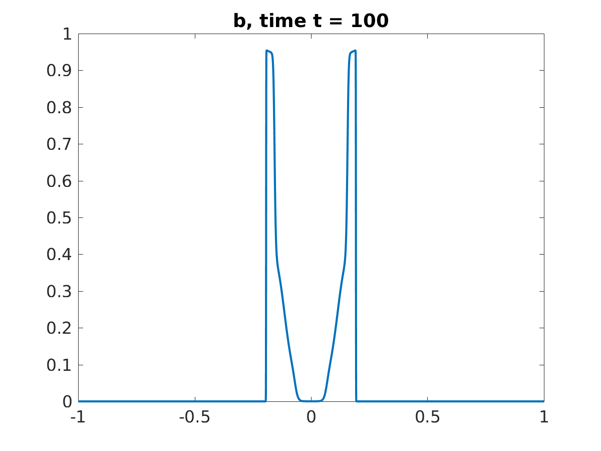
As a next step, we examine the dynamical behaviour of solutions. To this end we consider a situation where initially, two compactly supported bumbs of both and are centered at in the domain, see Figure 7. All subsequent simulations are done for and . First we examined the case and in which we observe unmixing of the two species first, before the two populations meet, see Figure 8. In the case and , we observe only a partial unmixing until the two densities meet, see Figure 9.
5.2 Examples in two spatial dimensions
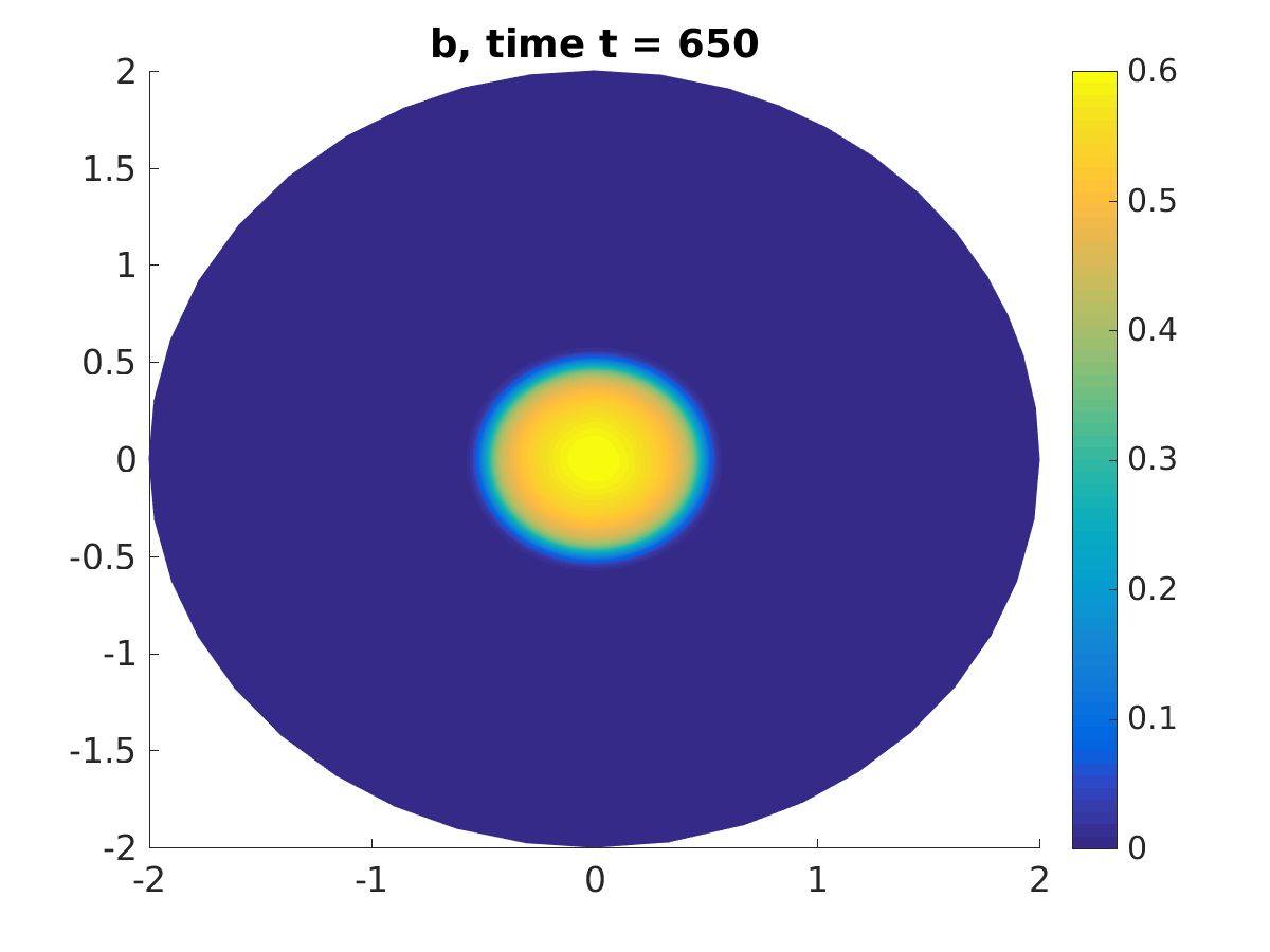
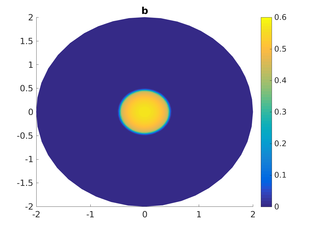
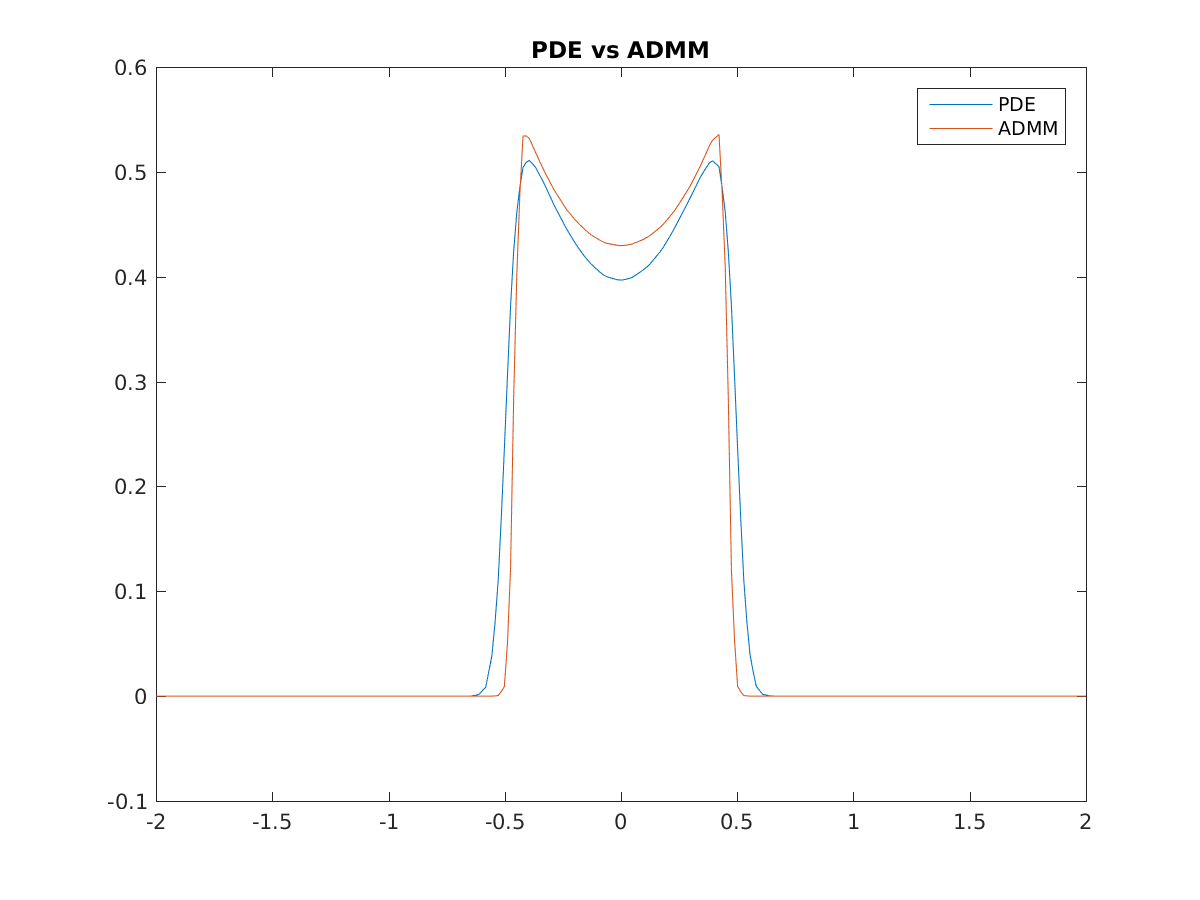
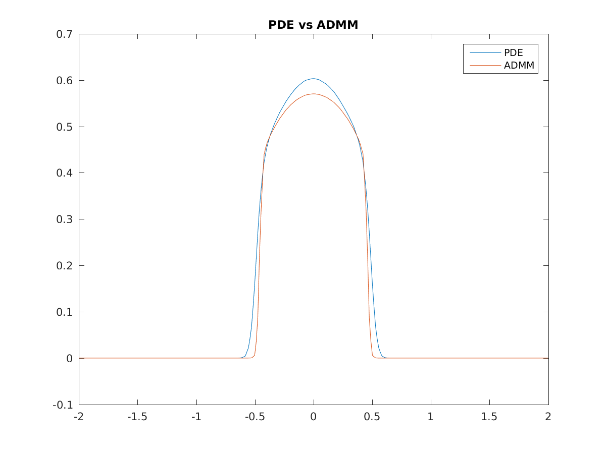
In two dimensions, we only present one example showing that for large , the solutions of the system seem in fact to converge to the minimizers obtained by the ADMM scheme. To this end, we chose again the case and and and used the solution of the PDE at time . The results are shown in figure 10. Note that our present results only ensure the existence of solution for arbitrary large yet finite time. However, we expect that these can be extended to the case and that we can in fact show convergence to stationary solutions by means of relative entropy methods.


6 Outlook: Coarsening Dynamics
In the following we further investigate the coarsening dynamics of the system (1.3), (1.4) as . Let us first of all discuss the case , which is characterized by a very large set of stationary solutions. Indeed, every pair with
| (6.1) |
is a stationary solution, but not necessarily stable under the dynamics. In the case for a single species, stability was characterized from an entropy condition in [21], noticing that the model for consists of nonlinear hyperbolic conservation laws with nonlocal terms. A generalization of the entropy condition to the system case seems out of reach, hence we revisit the single species case ( in our notation) and rederive the stability condition from an optimization argument. Intuitively a stationary state is stable if it is a local minimizer of the energy, and using a Lagrange multiplier for the mass constraint we easily arrive at the conditions
Thus, at an interface between a region with inside and outside the normal derivative of is nonpositive, which is exactly the entropy condition derived in [34, 21].
In the system case we find by analogous arguments with Lagrange parameters and for the masses
Hence we can effectively derive conditions on the sign of the normal derivatives of
on interfaces between regions with , , or (voids). On interfaces between red or blue and void the same analysis as in [21] applies, on interfaces between red and blue sign conditions on the derivatives of and need to hold simultaneously. Such stable configurations will lead to similar stationary solutions or metastable dynamics in the case of small positive .
We finally mention that for the coarsening of interfaces in the metastable case analogous laws as in [34, 21] can be derived by multiscale asymptotic expansions, whose details we leave to future research. In numerical experiments the coarsening dynamics is well observed, see Figure 8, where one obtains local unmixing followed by coarsening. In the case of small self-attraction as shown in Figure 9 a different kind of coarsening dynamics is obtained, which is not characterized by and attaining values close to , but a mixed phase is coarsening versus the void regions. In this case a further analysis is quite open and an interesting issue for the future.
Acknowledgements
JB and MB acknowledge support by ERC via Grant EU FP 7 - ERC Consolidator Grant 615216 LifeInverse. The work of JFP was supported by DFG via Grant 1073/1-2. The authors thank Alessio Brancolini, Benedikt Wirth and Caterina Ida Zeppieri (all WWU Münster) and Harald Garcke (University Regensburg) for useful discussions and links to literature. Furthermore, we thank the anonymous referees for many suggestions that substantially improved the paper.
References
- [1] Athmane Bakhta, Eric Cances, Virginie Ehrlacher, and Thomas Lelievre. Control of atom fluxes for the production of solar cell devices.
- [2] D. Balagué, J.A. Carrillo, T. Laurent, and G. Raoul. Nonlocal interactions by repulsive–attractive potentials: Radial ins/stability. Physica D: Nonlinear Phenomena, 260:5 – 25, 2013. Emergent Behaviour in Multi-particle Systems with Non-local Interactions.
- [3] Sisto Baldo. Minimal interface criterion for phase transitions in mixtures of Cahn-Hilliard fluids. In Annales de l’IHP Analyse non linéaire, volume 7, pages 67–90, 1990.
- [4] John W Barrett, James F Blowey, and Harald Garcke. On fully practical finite element approximations of degenerate Cahn-Hilliard systems. ESAIM: Mathematical Modelling and Numerical Analysis, 35(4):713–748, 2001.
- [5] Jacob Bedrossian. Global minimizers for free energies of subcritical aggregation equations with degenerate diffusion. Applied Mathematics Letters, 24(11):1927–1932, 2011.
- [6] Jacob Bedrossian, Nancy Rodríguez, and Andrea L. Bertozzi. Local and global well-posedness for aggregation equations and Patlak–Keller–Segel models with degenerate diffusion. Nonlinearity, 24(6):1683, 2011.
- [7] Judith Berendsen, Martin Burger, and Jan-Frederik Pietschmann. Videos of the one-dimensional dynamics. http://www.jfpietschmann.eu/nonlocal.
- [8] Andrea L. Bertozzi, Thomas Laurent, and Jesús Rosado. Lp theory for the multidimensional aggregation equation. Communications on Pure and Applied Mathematics, 64(1):45–83, 2011.
- [9] Andrea L Bertozzi and Dejan Slepcev. Existence and uniqueness of solutions to an aggregation equation with degenerate diffusion. Communications on Pure and Applied Analysis, 9(6):1617, 2009.
- [10] Silvia Boi, Vincenzo Capasso, and Daniela Morale. Modeling the aggregative behavior of ants of the species polyergus rufescens. Nonlinear Analysis: Real World Applications, 1(1):163–176, 2000.
- [11] Andrea Braides. -convergence for beginners, volume 22 of Oxford Lecture Series in Mathematics and its Applications. Oxford University Press, Oxford, 2002.
- [12] Lia Bronsard, Harald Garcke, and Barbara Stoth. A multi-phase Mullins–Sekerka system: Matched asymptotic expansions and an implicit time discretisation for the geometric evolution problem. Proceedings of the Royal Society of Edinburgh: Section A Mathematics, 128(03):481–506, 1998.
- [13] Maria Bruna and S. Jonathan Chapman. Diffusion of multiple species with excluded-volume effects. The Journal of chemical physics, 137(20):204116, 2012.
- [14] Maria Bruna and S. Jonathan Chapman. Excluded-volume effects in the diffusion of hard spheres. Physical Review E, 85(1):011103, 2012.
- [15] Martin Burger, Vincenzo Capasso, and Daniela Morale. On an aggregation model with long and short range interactions. Nonlinear Anal. Real World Appl., 8(3):939–958, 2007.
- [16] Martin Burger and Marco Di Francesco. Large time behavior of nonlocal aggregation models with nonlinear diffusion. Netw. Heterog. Media, 3(4):749–785, 2008.
- [17] Martin Burger, Marco Di Francesco, and Yasmin Dolak-Struss. The Keller-Segel model for chemotaxis with prevention of overcrowding: linear vs. nonlinear diffusion. SIAM J. Math. Anal., 38(4):1288–1315 (electronic), 2006.
- [18] Martin Burger, Marco Di Francesco, Simone Fagioli, and Angela Stevens. Segregated stationary solutions of a cross-diffusion system with nonlocal interaction. Preprint, 2016.
- [19] Martin Burger, Marco Di Francesco, and Marzena Franek. Stationary states of quadratic diffusion equations with long-range attraction. Commun. Math. Sci., 11(3):709–738, 2013.
- [20] Martin Burger, Marco Di Francesco, Jan-Frederik Pietschmann, and Bärbel Schlake. Nonlinear cross-diffusion with size exclusion. SIAM J. Math. Anal., 42(6):2842–2871, 2010.
- [21] Martin Burger, Yasmin Dolak-Struss, Christian Schmeiser, et al. Asymptotic analysis of an advection-dominated chemotaxis model in multiple spatial dimensions. Communications in Mathematical Sciences, 6(1):1–28, 2008.
- [22] Martin Burger, Razvan Fetecau, and Yanghong Huang. Stationary states and asymptotic behavior of aggregation models with nonlinear local repulsion. SIAM Journal on Applied Dynamical Systems, 13(1):397–424, 2014.
- [23] Martin Burger, Sabine Hittmeir, Helene Ranetbauer, and Marie-Therese Wolfram. Lane formation by side-stepping. SIAM Journal on Mathematical Analysis, 48(2):981–1005, 2016.
- [24] Martin Burger, Bärbel Schlake, and Marie-Therese Wolfram. Nonlinear Poisson–Nernst–Planck equations for ion flux through confined geometries. Nonlinearity, 25(4):961, 2012.
- [25] Vincent Calvez and José A Carrillo. Volume effects in the Keller–Segel model: energy estimates preventing blow-up. Journal de mathématiques pures et appliquées, 86(2):155–175, 2006.
- [26] José A. Cañizo, José A. Carrillo, and Francesco S. Patacchini. Existence of compactly supported global minimisers for the interaction energy. Arch. Ration. Mech. Anal., 217(3):1197–1217, 2015.
- [27] José A. Carrillo, Matias G. Delgadino, and Antoine Mellet. Regularity of local minimizers of the interaction energy via obstacle problems. Communications in Mathematical Physics, 343(3):747–781, 2016.
- [28] José A. Carrillo, M. Di Francesco, A. Figalli, T. Laurent, and D. Slepčev. Global-in-time weak measure solutions and finite-time aggregation for nonlocal interaction equations. Duke Math. J., 156(2):229–271, 2011.
- [29] José A. Carrillo, Sabine Hittmeir, Bruno Volzone, and Yao Yao. Nonlinear aggregation-diffusion equations: Radial symmetry and long time asymptotics. arXiv preprint arXiv:1603.07767, 2016.
- [30] Lincoln Chayes, Inwon Kim, and Yao Yao. An aggregation equation with degenerate diffusion: qualitative property of solutions. SIAM Journal on Mathematical Analysis, 45(5):2995–3018, 2013.
- [31] Yuxin Chen and Theodore Kolokolnikov. A minimal model of predator–swarm interactions. Journal of The Royal Society Interface, 11(94):20131208, 2014.
- [32] Rustum Choksi, Razvan C. Fetecau, and Ihsan Topaloglu. On minimizers of interaction functionals with competing attractive and repulsive potentials. Ann. Inst. H. Poincaré Anal. Non Linéaire, 32(6):1283–1305, 2015.
- [33] Marco Cicalese, Lucia De Luca, Matteo Novaga, and Marcello Ponsiglione. Ground states of a two phase model with cross and self attractive interactions, 2015.
- [34] Yasmin Dolak and Christian Schmeiser. The Keller–Segel model with logistic sensitivity function and small diffusivity. SIAM Journal on Applied Mathematics, 66(1):286–308, 2005.
- [35] Michael Dreher and Ansgar Jüngel. Compact families of piecewise constant functions in. Nonlinear Analysis: Theory, Methods & Applications, 75(6):3072 – 3077, 2012.
- [36] Janet Dyson, Stephen A Gourley, Rosanna Villella-Bressan, and Glenn F Webb. Existence and asymptotic properties of solutions of a nonlocal evolution equation modeling cell-cell adhesion. SIAM Journal on Mathematical Analysis, 42(4):1784–1804, 2010.
- [37] Charles M Elliott and Harald Garcke. Diffusional phase transitions in multicomponent systems with a concentration dependent mobility matrix. Physica D: Nonlinear Phenomena, 109(3):242–256, 1997.
- [38] L. C. Evans. Partial Differential Equations, volume 19 of Graduate Studies in Mathematics. American Mathematical Society, 1998.
- [39] Klemens Fellner and Gaël Raoul. Stable stationary states of non-local interaction equations. Mathematical Models and Methods in Applied Sciences, 20(12):2267–2291, 2010.
- [40] Harald Garcke, Britta Nestler, and Barbara Stoth. On anisotropic order parameter models for multi-phase systems and their sharp interface limits. Physica D: Nonlinear Phenomena, 115(1):87–108, 1998.
- [41] Harald Garcke, Amy Novick-Cohen, et al. A singular limit for a system of degenerate Cahn-Hilliard equations. Advances in Differential Equations, 5(4-6):401–434, 2000.
- [42] David Gilbarg and Neill Trudinger. Elliptic Partial Differential Equations of Second Order. Springer-Verlag, 1983.
- [43] Roland Glowinski, Stanley J. Osher, and Wotao (Eds.) Yin. Splitting Methods in Communication and Imaging, Science, and Engineering. Scientific Computation. Springer International Publishing, 2016.
- [44] Jens A. Griepentrog. On the unique solvability of a nonlocal phase separation problem for multicomponent systems. Banach Center Publications, WIAS preprint 898, 66:153–164, 2004.
- [45] Matthias Herz and Peter Knabner. Including van der Waals forces in diffusion-convection equations-modeling, analysis, and numerical simulations. arXiv preprint arXiv:1608.08431, 2016.
- [46] Magnus R. Hestenes. Multiplier and gradient methods. J. Optimization Theory Appl., 4:303–320, 1969.
- [47] Thomas Hillen and Kevin J. Painter. A user’s guide to pde models for chemotaxis. Journal of mathematical biology, 58(1-2):183–217, 2009.
- [48] M. Hinze, R. Pinnau, M. Ulbrich, and S. Ulbrich. Optimization with PDE constraints, volume 23 of Mathematical Modelling: Theory and Applications. Springer, New York, 2009.
- [49] Ansgar Jüngel. The boundedness-by-entropy method for cross-diffusion systems. Nonlinearity, 28(6):1963, 2015.
- [50] Gunnar Kaib. Stationary states of an aggregation equation with degenerate diffusion and bounded attractive potential. arXiv preprint arXiv:1604.07298, 2016.
- [51] Gary M Lieberman. Second order parabolic differential equations. World scientific, 1996.
- [52] Alexander Mogilner and Leah Edelstein-Keshet. A non-local model for a swarm. Journal of Mathematical Biology, 38(6):534–570, 1999.
- [53] Robert Nürnberg. Numerical simulations of immiscible fluid clusters. Applied Numerical Mathematics, 59(7):1612–1628, 2009.
- [54] Kevin J. Painter. Continuous models for cell migration in tissues and applications to cell sorting via differential chemotaxis. Bulletin of Mathematical Biology, 71(5):1117–1147, 2009.
- [55] Kevin J. Painter and Thomas Hillen. Volume-filling and quorum-sensing in models for chemosensitive movement. Can. Appl. Math. Quart, 10(4):501–543, 2002.
- [56] M. J. D. Powell. A method for nonlinear constraints in minimization problems. In R. Fletcher, editor, Optimization, pages 283–298. Academic Press, New York, 1969.
- [57] Bärbel Schlake. Mathematical Models for Particle Transport: Crowded Motion. PhD thesis, WWU Münster, 2011.
- [58] Robert Simione. Properties of Minimizers of Nonlocal Interaction Energy. ProQuest LLC, Ann Arbor, MI, 2014. Thesis (Ph.D.)–Carnegie Mellon University.
- [59] Robert Simione, Dejan Slepčev, and Ihsan Topaloglu. Existence of ground states of nonlocal-interaction energies. J. Stat. Phys., 159(4):972–986, 2015.
- [60] Matthew J Simpson, Kerry A Landman, and Barry D Hughes. Multi-species simple exclusion processes. Physica A: Statistical Mechanics and its Applications, 388(4):399–406, 2009.
- [61] Dejan Slepcev. Coarsening in nonlocal interfacial systems. SIAM Journal on Mathematical Analysis, 40(3):1029–1048, 2008.
- [62] Robert Stańczy. On an evolution system describing self-gravitating particles in microcanonical setting. Monatshefte für Mathematik, 162(2):197–224, 2011.
- [63] Jan-Eric Wurst. Hp-Finite Elements for PDE-Constrained Optimization. PhD thesis, 2015.
- [64] Nicola Zamponi and Ansgar Jüngel. Analysis of degenerate cross-diffusion population models with volume filling. In Annales de l’Institut Henri Poincare (C) Non Linear Analysis. Elsevier, 2015.
- [65] Jonathan Zinsl and Daniel Matthes. Transport distances and geodesic convexity for systems of degenerate diffusion equations. Calc. Var. Partial Differential Equations, 54(4):3397–3438, 2015.