Equivariant Perturbation in
Gomory and Johnson’s Infinite Group Problem.
V. Software for the continuous and discontinuous 1-row case

Abstract

We present software for investigations with cut-generating functions in the Gomory–Johnson model and extensions, implemented in the computer algebra system SageMath.

90C10; 90C11

1 Introduction

Consider the following question from the theory of linear inequalities over the reals: Given a (finite) system $Ax\leq b$, exactly which linear inequalities $\langle a,x\rangle\leq\beta$ are valid, i.e., satisfied for every $x$ that satisfies the given system? The answer is given, of course, by the Farkas Lemma, or, equivalently, by the strong duality theory of linear optimization. As is well-known, this duality theory is symmetric: The dual of a linear optimization problem is again a linear optimization problem, and the dual of the dual is the original (primal) optimization problem.

The question becomes much harder when all or some of the variables are constrained to be integers. The theory of valid linear inequalities here is called cutting plane theory. Over the past 60 years, a vast body of research has been carried out on this topic, the largest part of it regarding the polyhedral combinatorics of integer hulls of particular families of problems. The general theory again is equivalent to the duality theory of integer linear optimization problems. Here the dual objects are not linear, but superadditive (or subadditive) functionals, making the general form of this theory infinite-dimensional even though the original problem started out with only finitely many variables.

These superadditive (or subadditive) functionals appear in integer linear optimization in various concrete forms, for example in the form of dual-feasible functions [2], superadditive lifting functions [24], and cut-generating functions [9].

In the present paper, we describe some aspects of our software [18] for cut-generating functions in the classic 1-row Gomory–Johnson [14, 15] model. The model has a single parameter, a number $f\in\mathbb{R}\setminus\mathbb{Z}$. On the primal side of the model, one has finite-support functions $y\colon\mathbb{R}\to\mathbb{Z}_{+}$ that satisfy the group equation

$$\sum_{r\in\mathbb{R}}r\,y(r)\in f+\mathbb{Z}.$$ (1)

We omit any further discussion of the primal side and how it arises as an infinite-dimensional relaxation of integer linear optimization problems; we refer the reader to the recent survey [4, 5] for a complete exposition. Our software only works on the dual side, where the main objects of interest are the so-called minimal valid functions. By a characterization by Gomory–Johnson [14] (see also [4, Theorem 2.6]), they are the $\mathbb{Z}$-periodic functions $\pi\colon\mathbb{R}\to\mathbb{R}$ that satisfy the following conditions:

$$\pi(0)=0,\ \pi(f)=1$$ (2a)

$$\pi(x)\geq 0 \text{for }x\in\mathbb{R}$$ (2b)

$$\pi(x)+\pi(f-x)=1 \text{for }x\in\mathbb{R}$$ (symmetry condition) (2c)

$$\pi(x)+\pi(y)\geq\pi(x+y) \text{for }x,y\in\mathbb{R} \text{(subadditivity)}.$$ (2d)

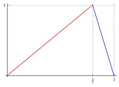
In the same way that finite-dimensional cutting plane theory has focused on finding families of facet-defining valid inequalities, a large part of the literature on the Gomory–Johnson model has focused on extreme functions. These are the minimal valid functions that are not a proper convex combination of other minimal valid functions. Figure 1–left shows the famous extreme function gmic, the cut-generating function of the Gomory mixed integer cut. It is convenient to rephrase the extremality condition in terms of perturbation functions. We say that a function $\tilde{\pi}\colon\mathbb{R}\to\mathbb{R}$ is an effective perturbation function for the minimal valid function $\pi$, if there exists $\epsilon>0$ such that $\pi\pm\epsilon\bar{\pi}$ are minimal valid functions. The effective perturbation functions form a vector space, denoted by $\tilde{\Pi}^{\pi}(\mathbb{R},\mathbb{Z})$; thus $\pi$ is extreme if and only if this space is trivial.

This paper is part of a series, dedicated to making the theory of cut-generating functions in the Gomory–Johnson model algorithmic. For the 1-row case, the focus lies on $\mathbb{Z}$-periodic piecewise linear functions $\pi$, which have an obvious finite representation in the computer. It is an easy observation that the conditions (2) for minimality are finitely checkable for such functions: Consider a $\mathbb{Z}^{2}$-periodic polyhedral complex $\Delta\mathcal{P}$ on $\mathbb{R}^{2}$ such that the subadditivity slack $\Delta\pi(x,y)=\pi(x)+\pi(y)-\pi(x+y)$ is a linear function on the relative interior of each face of $\Delta\mathcal{P}$. Then, in the continuous case, it suffices to check subadditivity (i.e., nonnegativity of $\Delta\pi$) on the vertices ($0$-dimensional faces) of this complex. In the discontinuous case, one additionally has to consider finitely many directional limits to the vertices.

In contrast to minimality, testing extremality is much more subtle. Making it algorithmic for various classes of functions is the main technical contribution of the present series of papers. In this project, the study of spaces of perturbation functions takes a central rôle.

A proof of extremality from the published literature follows a standard pattern, which can be phrased in terms of perturbation functions as follows. Take an effective perturbation function $\tilde{\pi}$; the goal is to show that $\tilde{\pi}=0$. Whenever $\Delta\pi(x,y)=0$ (additivity) holds for some $x,y$, the same is true for $\tilde{\pi}$. By applying reasoning from functional equations, in particular variants of the Gomory–Johnson Interval Lemma, to these additivity relations, one infers that $\tilde{\pi}$ is linear on certain intervals. If the intervals of linearity, which we refer to as covered intervals, cover the domain of $\tilde{\pi}$, then $\tilde{\pi}$ belongs to a finite-dimensional space of piecewise linear perturbation functions. In this case, a matrix computation suffices to decide whether $\tilde{\pi}=0$. However, it remained unclear whether these tools and this proof pattern were sufficient for deciding extremality in all cases.

In the first paper in the present series, Basu et al. [3], focusing on the 1-row Gomory–Johnson model, developed additional tools for piecewise linear functions with rational breakpoints and showed that a finite number of applications of these tools suffice for deciding extremality in the case of piecewise linear (possibly discontinuous) minimal valid functions with rational breakpoints. Thus, Basu et al. [3] obtained the first algorithm for testing extremality of a minimal valid function within this class.

This algorithm from [3] works using the grid $\frac{1}{q}\mathbb{Z}$, where $q$ is the least common multiple of all breakpoint denominators. In contrast, our software implements a grid-free variant. In the present paper, we provide a number of new results that underly the grid-free extremality test; they are generalizations of results from the literature. A practical benefit of our grid-free variant is that its empirical running time does not strongly depend on $q$. Moreover, it paves the way to computations with functions that have irrational breakpoints; this topic is further developed in [21, 17]. It is also the basis for computational investigations with parametric families of extreme functions in [23].

Our software is a tool that enables mathematical exploration and research in the domain of cut-generating functions. It can also be used in an educational setting, where it enables hands-on teaching about modern cutting plane theory based on cut-generating functions. It removes the limitations of hand-written proofs, which would be dominated by tedious case analysis.

Our software is written in Python, making use of the convenient and popular framework of the open-source computer algebra system SageMath. We begin our article with a brief overview about this system (section 2).

Next, in section 3, we describe the anatomy of our main objects, the $\mathbb{Z}$-periodic, possibly discontinuous piecewise linear functions $\pi\colon\mathbb{R}\to\mathbb{R}$, connecting the notation from the literature to relevant Python functions and methods. We also introduce the electronic compendium [20] of extreme functions found in the literature.

The algorithmic minimality and extremality tests make use of certain 2-dimensional diagrams, associated with the polyhedral complex $\Delta\mathcal{P}$, which record the subadditivity and additivity properties of a given function $\pi$. In section 4 we give a definition of this complex and introduce these diagrams. Then, in section 5, we describe the details of the automatic minimality test. In section 6 we explain the computation of the covered intervals for a given minimal valid function. This is one of the ingredients of the extremality test, which we explain in section 7.

In sections 8 and 9, we describe transformations that can be applied to extreme functions and functionality of our software for the closely related finite group relaxation model. We end our article with some comments regarding the documentation and test suite of our software (section 10).

The first version of our software [18] was written by the first author, C. Y. Hong, during a Research Experience for Undergraduates in summer 2013. It was later revised and extended by M. Köppe and again by Y. Zhou. The latter added the electronic compendium and code that handles the case of discontinuous functions. Version 0.9 of our software was released in 2014 to accompany the survey [4, 5]; the software has received continuous updates by the second and third authors since. Two further undergraduate students contributed to our software. P. Xiao contributed some documentation and tests. M. Sugiyama contributed additional functions to the compendium, and added code for superadditive lifting functions.

2 About SageMath as a research and education platform in optimization

Our software is written in Python, making use of the convenient framework of the open-source computer algebra system SageMath [28]. It can be run on a local installation of SageMath, or online via SageMathCloud.

We briefly explain what sets SageMath apart from other computer algebra systems, making it suitable as a research platform in optimization. First, its surface language is the popular programming language Python, altered only in a minimal way by the SageMath pre-parser to provide some syntactic sugar for mathematical notation. This in contrast to systems such as Maple and Mathematica, which have their own idiosyncratic surface languages. Second, while SageMath itself is written in Python and Cython, it interfaces to a large number of open-source and commercial software packages, and as a principle delegates all computations to a state-of-the-art library when possible, rather than using its own implementation. Relevant features for research and education in optimization are the following:

• the interfaces to major numerical mixed-integer linear optimization solvers, CPLEX, Gurobi, COIN-OR CBC, in addition to GLPK, which is used as the default solver, as well as an interface to the convex optimization solver CVXOPT;

• an interface to the exact (rational arithmetic) mixed integer linear optimization solver in the Parma Polyhedra Library;

• a didactical implementation of the simplex method that is able to work over general ordered fields, with a didactical implementation of cutting-plane methods [1, #18805] in development;

• a textbook view on the numerical solvers [1, #18804] in development;

• interfaces to state-of-the-art polyhedral computation software, including the Parma Polyhedra Library, cddlib, TOPCOM, Normaliz, and polymake, as well as an implementation of polyhedral computation methods for general ordered fields;

• interfaces to state-of-the-art lattice-point computation software, LattE integrale, 4ti2, and Normaliz, as well as its own implementation of lattice-point enumeration.

3 Continuous and discontinuous piecewise linear $\mathbb{Z}$-periodic functions

The main objects of our code are the $\mathbb{Z}$-periodic functions $\pi\colon\mathbb{R}\to\mathbb{R}$. Our code is limited to the case of piecewise linear functions, which are allowed to be discontinuous; see the definition below. In our code, the periodicity of the functions is implicit; the functions are represented by their restriction to the interval $[0,1]$. They can be constructed in various ways using Python functions named piecewise_function_from_breakpoints_and_values etc.

Our software includes an electronic compendium, which is up-to-date with our knowledge on extreme functions. It is accessible by the Python module named extreme_functions. One can use the help system of Sage, by typing the name of an extreme function followed by a question mark, to access the documentation string of the function, which provides a discussion of parameters, bibliographic information, etc.; see Table 2. Table 1 shows the source code of gmic in the electronic compendium. It constructs the piecewise linear extreme function from the breakpoints and the values at the breakpoints. This function is the cut-generating function of the famous Gomory mixed-integer cut [12].

The source code of the electronic compendium provides many other examples of constructions of functions. An early version of the electronic compendium has been described in the paper [20]. The reader may also refer to the survey [4, Tables 1–4], which shows the graphs of these functions for default parameters next to their names. Since the publication of [20, 4], additional extreme functions have been implemented in the compendium. They include the family of extreme functions with an arbitrary number of slopes (extreme_functions.bcdsp_arbitrary_slope) that was recently constructed by Basu–Conforti–Di Summa–Paat [8], the family of $\text{CPL}_{3}^{=}$ functions (mlr_cpl3_...) that was obtained by Miller–Li–Richard [25] from an approximate lifting of superadditive functions, and new parametric families and sporadic extreme functions (kzh_...) that were found by Köppe–Zhou [22, 23] using computer-based search.

Table 1: The construction of the gmic function in the compendium.

Ψdef gmic(f=4/5, field=None, conditioncheck=True): Ψ"(docstring elided to save space)" Ψif conditioncheck and not bool(0 < f < 1): ΨΨraise ValueError, "Bad parameters. Unable to construct the function." Ψgmi_bkpt = [0,f,1] Ψgmi_values = [0,1,0] Ψreturn piecewise_function_from_breakpoints_and_values(gmi_bkpt, gmi_values, field=field) Ψ

A piecewise linear function $\pi$ can be plotted using the standard SageMath function plot($\pi$), or using our function plot_with_colored_slopes($\pi$), which assigns a different color to each different slope value that a linear piece takes.

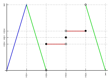
Random piecewise linear functions can be generated by calling the Python function named random_piecewise_function. By specifying the parameters, one obtains random continuous or discontinuous piecewise linear functions with prescribed properties, which could be useful to experimentation and exploration. Figure 1–right shows a random discontinuous function generated by

Ψh = random_piecewise_function(xgrid=5, ygrid=5, continuous_proba=1/3, symmetry=True). Ψ

This particular discontinuous function can also be set up by either of the following commands.

Ψh = piecewise_function_from_breakpoints_and_limits(bkpt=[0, 1/5, 2/5, 3/5, 4/5, 1], Ψ limits=[(0, 0, 0), (1, 1, 1), (2/5, 2/5, 0), (1/2, 3/5, 2/5), (3/5, 1, 3/5), (0, 0, 0)]) Ψh = piecewise_function_from_breakpoints_and_limits(bkpt=[0, 1/5, 2/5, 3/5, 4/5, 1], Ψ limits=[{-1:0, 0:0, 1:0}, {-1:1, 0:1, 1:1}, {-1:0, 0:2/5, 1:2/5}, Ψ {-1:2/5, 0:1/2, 1:3/5}, {-1:3/5, 0:3/5, 1:1}, {-1:0, 0:0, 1:0}]) Ψ

Figure 1: Two piecewise linear functions, as plotted by the command plot_with_colored_slopes(h). Left, continuous extreme function h = gmic(). Right, random discontinuous function h = equiv5_random_discont_1(), generated by random_piecewise_function(xgrid=5, ygrid=5, continuous_proba=1/3, symmetry=True).

In the following, we connect to the systematic notation introduced in [3, section 2.1]; see also [4, 5]. We suppress the details of the internal representation of a $\mathbb{Z}$-periodic piecewise linear function $\pi$ in our code; instead we explain the main ways in which the data of the function are accessed; see Table 2 for a sample Sage session.

$\pi$.end_points()

is a list $0=x_{0}<x_{1}<\dots<x_{n-1}<x_{n}=1$ of possible breakpoints of the function in $[0,1]$. In the notation from [3, 4, 5], these endpoints are extended periodically as $B=\{\,x_{0}+t,x_{1}+t,\dots,x_{n-1}+t:t\in\mathbb{Z}\,\}$. Then the set of 0-dimensional faces is defined to be the collection of singletons, $\bigl{\{}\,\{x\}:x\in B\,\bigr{\}}$, and the set of one-dimensional faces to be the collection of closed intervals, $\bigl{\{}\,[x_{i}+t,x_{i+1}+t]:i=0,\dots,{n-1}\text{ and }t\in\mathbb{Z}\,\bigr{\}}.$ Together, we obtain $\mathcal{P}=\mathcal{P}_{B}$, a locally finite polyhedral complex, periodic modulo $\mathbb{Z}$.

$\pi$.values_at_end_points()

is a list of the function values $\pi(x_{i})$, $i=0,\dots,n$. This list is most useful for continuous piecewise linear functions, as indicated by $\pi$.is_continuous(), in which case the function is defined on the intervals $[x_{i},x_{i+1}]$ by linear interpolation.

$\pi$.limits_at_end_points()

provides data for the general, possibly discontinuous case in the form of a list limits of 3-tuples, with

limits[$$i =\pi(x_{i})$$][0]

limits[$$i =\pi(x_{i}^{+})=\lim_{x\to x_{i},x>x_{i}}\pi(x)$$][1]

limits[$$i =\pi(x_{i}^{-})=\lim_{x\to x_{i},x<x_{i}}\pi(x).$$][-1]

The function is defined on the open intervals $(x_{i},x_{i+1})$ by linear interpolation of the limit values $\pi(x_{i}^{+})$, $\pi(x_{i+1}^{-})$.

$\pi$($x$) and $\pi$.limits($x$)

evaluate the function at $x$ and provide the 3-tuple of its limits at $x$, respectively.

$\pi$.which_function($x$)

returns a linear function, denoted $\pi_{I}\colon\mathbb{R}\to\mathbb{R}$ in [3, 4, 5], where $I$ is the smallest face of $\mathcal{P}$ containing $x$, so $\pi(x)=\pi_{I}(x)$ for $x\in\operatorname{rel\,int}(I)$.

Table 2: A sample Sage session, illustrating the basic use of a piecewise linear function and the help system.

Ψ## First load the code. Ψsage: import igp; from igp import * ΨINFO: 2016-08-08 16:49:21,594 Welcome to the infinite-group-relaxation-code. DON’T PANIC. See demo.sage for instructions. Ψ Ψ## The documentation string of each function reveals its optional arguments, usage examples, and bibliographic information. Ψsage: gmic? Ψ[...] ΨSignature: gmic(f=4/5, field=None, conditioncheck=True) ΨDocstring: Ψ Summary: Ψ * Name: GMIC (Gomory mixed integer cut); Ψ Ψ * Infinite (or Finite); Dim = 1; Slopes = 2; Continuous; Analysis of subadditive polytope method; Ψ Ψ * Discovered [55] p.7-8, Eq.8; Ψ Ψ * Proven extreme (for infinite group) [60] p.377, thm.3.3; (finite group) [57] p.514, Appendix 3. Ψ Ψ * (Although only extremality has been established in literature, the same proof shows that) gmic is a facet. Ψ Ψ Parameters: Ψ f (real) in (0,1). Ψ Ψ Examples: Ψ [61] p.343, Fig. 1, Example 1 Ψ Ψ sage: logging.disable(logging.INFO) # Suppress output in automatic tests. Ψ sage: h = gmic(4/5) Ψ sage: extremality_test(h, False) Ψ True Ψ Ψ Reference: Ψ [55]: R.E. Gomory, An algorithm for the mixed integer problem, Tech. Report RM-2597, RAND Corporation, 1960. Ψ Ψ [57]: R.E. Gomory, Some polyhedra related to combinatorial problems, Linear Algebra and its Application 2 (1969) 451-558. Ψ [60]: R.E. Gomory and E.L. Johnson, Some continuous functions related to corner polyhedra, part II, Ψ Mathematical Programming 3 (1972) 359-389. Ψ Ψ [61]: R.E. Gomory and E.L. Johnson, T-space and cutting planes, Mathematical Programming 96 (2003) 341-375. Ψ Ψ## We load the GMIC function and store it in variable h. Ψsage: h = gmic() ΨINFO: 2016-08-08 16:51:31,048 Rational case. Ψ## We query the data of the GMIC function. Ψsage: h.end_points() Ψ[0, 4/5, 1] Ψsage: h.values_at_end_points() Ψ[0, 1, 0] Ψsage: h(4/5) Ψ1 Ψsage: h.which_function(1/2) Ψ<FastLinearFunction 5/4*x> Ψ## Plot the function. Ψsage: plot_with_colored_slopes(h) Ψ Ψ## Next, we construct a discontinuous piecewise linear function and query its data. Ψsage: h = piecewise_function_from_breakpoints_and_limits(bkpt=[0, 1/5, 2/5, 3/5, 4/5, 1], ΨΨ limits=[(0, 0, 0), (1, 1, 1), (2/5, 2/5, 0), (1/2, 3/5, 2/5), (3/5, 1, 3/5), (0, 0, 0)]) Ψsage: h.limits_at_end_points() Ψ[[0, 0, 0], Ψ [1, 1, 1], Ψ [2/5, 2/5, 0], Ψ [1/2, 3/5, 2/5], Ψ [3/5, 1, 3/5], Ψ [0, 0, 0]] Ψ

4 The diagrams of the decorated 2-dimensional polyhedral complex $\Delta\mathcal{P}$

We now describe certain 2-dimensional diagrams which record the subadditivity and additivity properties of a given function. These diagrams, in the continuous case, have appeared extensively in [4, 5, 20]. An example for the discontinuous case appeared in [20]. We have engineered these diagrams from earlier forms that can be found in [16] (for the discussion of the merit_index) and in [3], to become power tools for the modern cutgeneratingfunctionologist. Not only is the minimality of a given function immediately apparent on the diagram, but also the extremality proof for a given class of piecewise minimal valid functions follows a standard pattern that draws from these diagrams. See [5, prelude] and [20, sections 2 and 4] for examples of such proofs.

4.1 The polyhedral complex and its faces

Following [3, 4, 5], we introduce the function

$$\Delta\pi\colon\mathbb{R}\times\mathbb{R}\to\mathbb{R},\quad\Delta\pi(x,y)=\pi(x)+\pi(y)-\pi(x+y),$$

which measures the slack in the subadditivity condition. Thus, if $\Delta\pi(x,y)<0$, subadditivity is violated at $(x,y)$; if $\Delta\pi(x,y)=0$, additivity holds at $(x,y)$; and if $\Delta\pi(x,y)>0$, we have strict subadditivity at $(x,y)$. The piecewise linearity of $\pi(x)$ induces piecewise linearity of $\Delta\pi(x,y)$. To express the domains of linearity of $\Delta\pi(x,y)$, and thus domains of additivity and strict subadditivity, we introduce the two-dimensional polyhedral complex $\Delta\mathcal{P}$. The faces $F$ of the complex are defined as follows. Let $I,J,K\in\mathcal{P}$, so each of $I,J,K$ is either a breakpoint of $\pi$ or a closed interval delimited by two consecutive breakpoints. Then

$$F=F(I,J,K)=\left\{\,(x,y)\in\mathbb{R}\times\mathbb{R}\,:\,x\in I,\,y\in J,\,x+y\in K\,\right\}.$$

In our code, a face is represented by an instance of the class Face. It is constructed from $I,J,K$ and is represented by the list of vertices of $F$ and its projections $I^{\prime}=p_{1}(F)$, $J^{\prime}=p_{2}(F)$, $K^{\prime}=p_{3}(F)$, where $p_{1},p_{2},p_{3}\colon\mathbb{R}\times\mathbb{R}\to\mathbb{R}$ are defined as $p_{1}(x,y)=x$, $p_{2}(x,y)=y$, $p_{3}(x,y)=x+y$. The vertices $\operatorname{vert}(F)$ are obtained by first listing the basic solutions $(x,y)$ where $x$, $y$, and $x+y$ are fixed to endpoints of $I$, $J$, and $K$, respectively, and then filtering the feasible solutions. The three projections are then computed from the list of vertices. Due to the $\mathbb{Z}$-periodicity of $\pi$, we can represent a face as a subset of $[0,1]\times[0,1]$. See Figure 2 for an example. Because of the importance of the projection $p_{3}(x,y)=x+y$, it is convenient to imagine a third, $(x+y)$-axis in addition to the $x$-axis and the $y$-axis, which traces the bottom border for $0\leq x+y\leq 1$ and then the right border for $1\leq x+y\leq 2$. To make room for this new axis, the $x$-axis should be drawn on the top border of the diagram.

Figure 2: An example of a face $F=F(I,J,K)$ of the 2-dimensional polyhedral complex $\Delta\mathcal{P}$, set up by F = Face([[0.2, 0.3], [0.75, 0.85], [1, 1.2]]). It has vertices (blue) $(0.2,0.85)$, $(0.3,0.75)$, $(0.3,0.85)$, $(0.2,0.8)$, $(0.25,0.75)$, whereas the other basic solutions (red) $(0.2,0.75)$, $(0.2,1)$, $(0.3,0.9)$, $(0.35,0.85)$, $(0.45,0.75)$ are filtered out because they are infeasible. The face $F$ has projections (gray shadows) $I^{\prime}=p_{1}(F)=[0.2,0.3]$ (top border), $J^{\prime}=p_{2}(F)=[0.75,0.85]$ (left border), and $K^{\prime}=p_{3}(F)=[1,1.15]$ (right border). Note that $K^{\prime}\subsetneq K$.

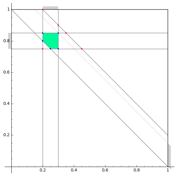
4.2 plot_2d_diagram_with_cones

We now explain the first version of the 2-dimensional diagrams, plotted by the function plot_2d_diagram_with_cones($\pi$); see Figure 3.

Figure 3: Two diagrams of functions and their polyhedral complexes $\Delta\mathcal{P}$ with colored cones at $\operatorname{vert}(\Delta\mathcal{P})$, as plotted by the command plot_2d_diagram_with_cones(h). Left, continuous function h = not_minimal_2(). Right, random discontinuous function h = equiv5_random_discont_1().

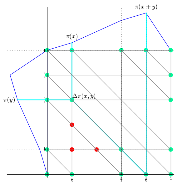
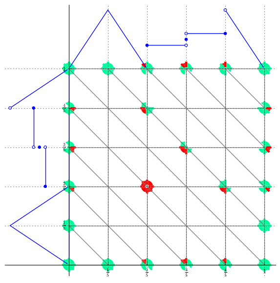
At the border of these diagrams, the function $\pi$ is shown twice (blue), along the $x$-axis (top border) and along the $y$-axis (left border). The solid grid lines in the diagrams are determined by the breakpoints of $\pi$: vertical, horizontal and diagonal grid lines correspond to values where $x$, $y$ and $x+y$ are breakpoints of $\pi$, respectively. The vertices of the complex $\Delta\mathcal{P}$ are the intersections of these grid lines.

In the continuous case, we indicate the sign of $\Delta\pi(x,y)$ for all vertices by colored dots on the diagram: red indicates $\Delta\pi(x,y)<0$ (subadditivity is violated); green indicates $\Delta\pi(x,y)=0$ (additivity holds).

Example 4.0.

In Figure 3 (left), showing the 2-dimensional diagram of the function $\pi=\texttt{not\char 95\relax\allowbreak minimal\char 95\relax\allowbreak 2()}$, the vertex $(x,y)=(\frac{1}{5},\frac{3}{5})$ is marked green, since

$$\Delta\pi(\tfrac{1}{5},\tfrac{3}{5}) =\pi(\tfrac{1}{5})+\pi(\tfrac{3}{5})-\pi(\tfrac{4}{5})=\tfrac{1}{5}+\tfrac{4}{5}-1=0.$$

In the discontinuous case, beside the subadditivity slack $\Delta\pi(x,y)$ at a vertex $(x,y)$, one also needs to study the limit value of $\Delta\pi$ at the vertex $(x,y)$ approaching from the interior of a face $F\in\Delta\mathcal{P}$ containing the vertex $(x,y)$. This limit value is defined by

$$\Delta\pi_{F}(x,y)=\lim_{\begin{subarray}{c}(u,v)\to(x,y)\\ (u,v)\in\operatorname{rel\,int}(F)\end{subarray}}\Delta\pi(u,v),\quad\text{where }F\in\Delta\mathcal{P}\text{ such that }(x,y)\in F.$$

We indicate the sign of $\Delta\pi_{F}(x,y)$ by a colored cone inside $F$ pointed at the vertex $(x,y)$ on the diagram. There could be up to $12$ such cones (including rays for one-dimensional faces $F$) around a vertex $(x,y)$.

Example 4.0.

In Figure 3 (right), showing the 2-dimensional diagram of the function $\pi=\texttt{equiv5\char 95\relax\allowbreak random\char 95\relax\allowbreak discont\char 95\relax\allowbreak 1()}$, the lower right corner $(x,y)=(\frac{2}{5},\frac{4}{5})$ of the face $F=F(I,J,K)$ with $I=[\frac{1}{5},\frac{2}{5}]$, $J=[\frac{4}{5},1]$, $K=[1,\frac{6}{5}]$ is green, since

$$\Delta\pi_{F}(x,y) =\lim_{\begin{subarray}{c}(u,v)\to(\frac{2}{5},\frac{4}{5})\\ (u,v)\in\operatorname{rel\,int}(F)\end{subarray}}\Delta\pi(u,v)$$

$$=\lim_{u\to\frac{2}{5},\;u<\frac{2}{5}}\pi(u)+\lim_{v\to\frac{4}{5},\;v>\frac{4}{5}}\pi(v)-\lim_{w\to\frac{6}{5},\;w<\frac{6}{5}}\pi(w)$$

$$=\pi(\tfrac{2}{5}^{-})+\pi(\tfrac{4}{5}^{+})-\pi(\tfrac{1}{5}^{-})\quad\text{(as }\pi(\tfrac{6}{5}^{-})=\pi(\tfrac{1}{5}^{-})\text{ by periodicity)}$$

$$=0+1-1=0.$$

The horizontal ray to the left of the same vertex $(x,y)=(\frac{2}{5},\frac{4}{5})$ is red, because approaching from the one-dimensional face $F^{\prime}=F(I^{\prime},J^{\prime},K^{\prime})$ that contains $(x,y)$, with $I^{\prime}=[\frac{1}{5},\frac{2}{5}]$, $J^{\prime}=\{\frac{4}{5}\}$, $K^{\prime}=[1,\frac{6}{5}]$, we have the limit value

$$\Delta\pi_{F^{\prime}}(x,y)=\lim_{\begin{subarray}{c}(u,v)\to(\frac{2}{5},\frac{4}{5})\\ (u,v)\in\operatorname{rel\,int}(F^{\prime})\end{subarray}}\Delta\pi(u,v)=\lim_{\begin{subarray}{c}u\to\frac{2}{5}\\ u<\frac{2}{5}\end{subarray}}\pi(u)+\pi(\tfrac{4}{5})-\lim_{\begin{subarray}{c}w\to\frac{6}{5}\\ w<\frac{6}{5}\end{subarray}}\pi(w)=0+\tfrac{3}{5}-1<0.$$

4.3 plot_2d_diagram and additive faces

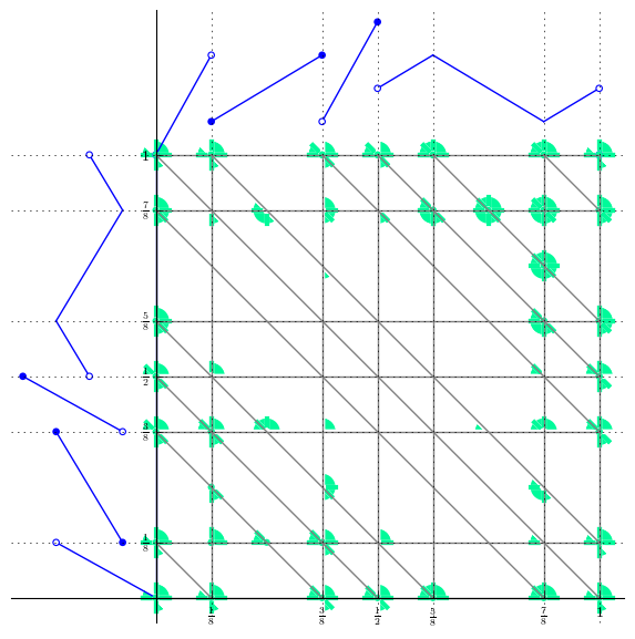
Now assume that $\pi$ is a subadditive function. Then there are no red dots or cones on the above diagram of the complex $\Delta\mathcal{P}$. See Figure 4 (left) and Figure 5 (left) for illustrations of the continuous and discontinuous cases.

Figure 4: Diagrams of $\Delta\mathcal{P}$ of a continuous function h = example7slopecoarse2(), with (left) additive vertices as plotted by the command plot_2d_diagram_with_cones(h); (right) maximal additive faces as plotted by the command plot_2d_diagram(h).

Figure 5: Diagrams of $\Delta\mathcal{P}$ of a discontinuous function h = hildebrand_discont_3_slope_1(), with (left) additive limiting cones as plotted by the command plot_2d_diagram_with_cones(h); (right) additive faces as plotted by the command plot_2d_diagram(h).

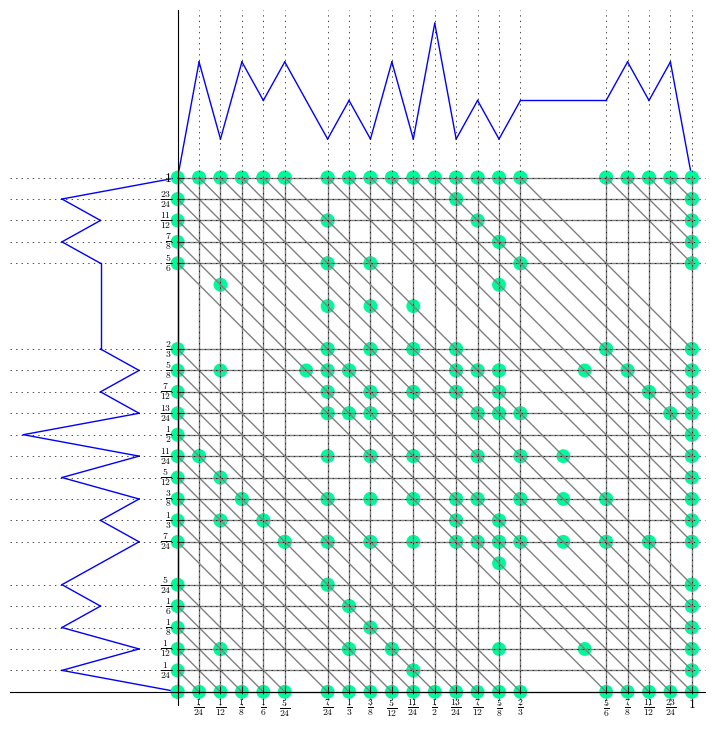
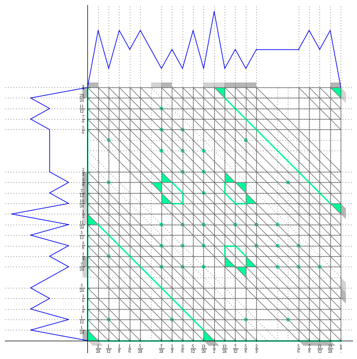
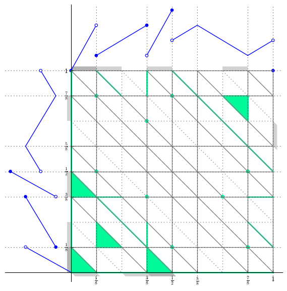
For a continuous subadditive function $\pi$, we say that a face $F\in\Delta\mathcal{P}$ is additive if $\Delta\pi=0$ over all $F$. Note that $\Delta\pi$ is affine linear over $F$, and so the face $F$ is additive if and only if $\Delta\pi(x,y)=0$ for all $(x,y)\in\operatorname{vert}(F)$. It is clear that any subface $E$ of an additive face $F$ ($E\subseteq F$, $E\in\Delta\mathcal{P}$) is still additive. Thus the additivity domain of $\pi$ can be represented by the list of inclusion-maximal additive faces of $\Delta\mathcal{P}$; see [4, Lemma 3.12]. This list is computed by generate_maximal_additive_faces($\pi$), whose algorithm will be explained in Appendix A.

For a discontinuous subadditive function $\pi$, we say that a face $F\in\Delta\mathcal{P}$ is additive if $F$ is contained in a face $F^{\prime}\in\Delta\mathcal{P}$ such that $\Delta\pi_{F^{\prime}}(x,y)=0$ for any $(x,y)\in F$. Since $\Delta\pi$ is affine linear in the relative interiors of each face of $\Delta\mathcal{P}$, the last condition is equivalent to $\Delta\pi_{F^{\prime}}(x,y)=0$ for any $(x,y)\in\operatorname{vert}(F)$. Depending on the dimension of $F$, we do the following.

1. Let $F$ be a two-dimensional face of $\Delta\mathcal{P}$. If $\Delta\pi_{F}(x,y)=0$ for any $(x,y)\in\operatorname{vert}(F)$, then $F$ is additive. Visually on the 2d-diagram with cones, each vertex of $F$ has a green cone sitting inside $F$.

2. Let $F$ be a one-dimensional face, i.e., an edge of $\Delta\mathcal{P}$. Let $(x_{1},y_{1}),(x_{2},y_{2})$ be its vertices. Besides $F$ itself, there are two other faces $F_{1},F_{2}\in\Delta\mathcal{P}$ that contain $F$. If $\Delta\pi_{F^{\prime}}(x_{1},y_{1})=\Delta\pi_{F^{\prime}}(x_{2},y_{2})=0$ for $F^{\prime}=F$, $F_{1}$, or $F_{2}$, then the edge $F$ is additive.

3. Let $F$ be a zero-dimensional face of $\Delta\mathcal{P}$, $F=\{(x,y)\}$. If there is a face $F^{\prime}\in\Delta\mathcal{P}$ such that $(x,y)\in F^{\prime}$ and $\Delta\pi_{F^{\prime}}(x,y)=0$, then $F$ is additive. Visually on the 2d-diagram with cones, the vertex $(x,y)$ is green or there is a green cone pointing at $(x,y)$.

On the diagrams in Figure 4 (right) and Figure 5 (right), the additive faces are shaded in green. The projections $p_{1}(F)$, $p_{2}(F)$, and $p_{3}(F)$ of a two-dimensional additive face $F$ are shown as gray shadows on the $x$-, $y$- and $(x+y)$-axes of the diagram, respectively. These projections become important in the computation of covered intervals (section 6 below).

The area of the additive faces of $\pi$ is related to the notion of merit index defined by Gomory and Johnson in [16]. For a minimal valid function $\pi$, the merit index is defined as twice the area of the additivity domain $\{(x,y)\in[0,1]^{2}\colon\Delta\pi(x,y)=0\}$ of $\pi$. This index, available as merit_index in our code, was proposed as a quantitative measure of strength of minimal valid functions. For example, the merit index of $\pi=\texttt{gmic}(f)$ is $2f^{2}-2f+1$.

5 Minimality test

The Python function minimality_test($\pi$, $f$) implements a fully automatic test whether a given function is a minimal valid function, using the information that the described 2-dimensional diagrams visualize. The algorithm is equivalent to the one described, in the setting of discontinuous pseudo-periodic superadditive functions, in Richard, Li, and Miller [27, Theorem 22].

Let $\pi$ be a piecewise linear $\mathbb{Z}$-periodic function and let $f\in[0,1]$. The command minimality_test($\pi$, $f$) verifies the characterization of minimal functions by Gomory–Johnson [14] that we mentioned in the introduction, returning True if and only if the conditions (2a–2d) are satisfied.

Note that because the given function $\pi$ is piecewise linear and $\mathbb{Z}$-periodic, the conditions (2b) and (2c) only need to be checked on the breakpoints (including the limits) of $\pi$ in $[0,1]$, namely, for $x\in\{x_{0},x_{1},\dots,x_{n},x_{0}^{+},x_{1}^{+},\dots,x_{n}^{+},x_{0}^{-},x_{1}^{-},\dots,x_{n}^{-}\}$. In regards to the subadditivity condition (2d), it suffices to check $\Delta\pi(x,y)\geq 0$ at the vertices $(x,y)$ of the 2-dimensional polyhedral complex $\Delta\mathcal{P}$ of $\pi$, including the limit values $\Delta\pi_{F}(x,y)$ when $\pi$ is a discontinuous function. The sign of $\Delta\pi$ is indicated by colors on the diagram plot_2d_diagram_with_cones($\pi$): if the diagram does not contain anything in red, then $\pi$ satisfies the subadditivity condition (2d). One can further restrict to the upper-left triangular part of $\Delta\mathcal{P}$ where $x\leq y$, since $\Delta\pi(x,y)=\Delta\pi(y,x)$ for any $x,y\in\mathbb{R}$.

It is clear that a minimal valid function $\pi$ satisfies $\pi(f)=1$. If the value of the optional argument f is not provided, then minimality_test($\pi$) uses $f=$ find_f($\pi$), which returns the first breakpoint $x_{i}\in[0,1]$ of $\pi$ such that $\pi(x_{i})=1$. Note that if a minimal valid function $\pi$ has distinct breakpoints $x_{i},x_{j}\in[0,1]$ such that $\pi(x_{i})=\pi(x_{j})=1$, then by the symmetry condition (2c), there exists $b\in(0,1)$ such that $\pi(b)=0$. In this case, the following lemma implies that $\pi$ is actually a $\frac{1}{q}\mathbb{Z}$-periodic function. Therefore, one can set $f$ to the first $x_{i}$ with $\pi(x_{i})=1$ without loss of generality.

Lemma 5.0.

Let $\pi$ be a piecewise linear $\mathbb{Z}$-periodic function that is minimal valid. If $\pi(b)=0$ for some $b\not\in\mathbb{Z}$, then $b\in\mathbb{Q}$ and $\pi$ is $\frac{1}{q}\mathbb{Z}$-periodic, where $q$ denotes the positive denominator of $b$ written as an irreducible fraction.

Proof.

Since the function $\pi$ is non-negative and subadditive, one can show by induction that $\pi(nb)=0$ for any integer $n$. Suppose that $b\not\in\mathbb{Q}$. The minimal valid function $\pi$ is $0$ on the set $b\mathbb{Z}$ and is $1$ on the set $f-b\mathbb{Z}$, where both sets are dense in $\mathbb{R}/\mathbb{Z}$. This contradicts the piecewise linearity of $\pi$. Therefore, $b\in\mathbb{Q}$. Let $p\in\mathbb{Z}$ and $q\in\mathbb{Z}_{+}$ such that $\gcd(p,q)=1$ and $b=\frac{p}{q}$. There exists $r\in\mathbb{Z}_{+}$ such that $rp\equiv 1\pmod{q}$. We have that $0=r\pi(b)\geq\pi(rb)=\pi(\frac{1}{q})$, and hence $\pi(\frac{1}{q})=0$. Similarly, we have that $\pi(-\frac{1}{q})=0$. Let $x\in\mathbb{R}$. By subadditivity, $\pi(x)+\pi(\frac{1}{q})\geq\pi(x+\frac{1}{q})$ and $\pi(x+\frac{1}{q})+\pi(-\frac{1}{q})\geq\pi(x)$. Therefore, $\pi(x)=\pi(x+\frac{1}{q})$. We conclude that the function $\pi$ is $\frac{1}{q}\mathbb{Z}$-periodic. ∎

If the minimality_test is called with the optional argument show_plots=True (default: False), then it shows the diagram of $\Delta\mathcal{P}$ illustrating the sign of $\Delta\pi(x,y)$ by colors.

6 Connected components of covered intervals

An additive face implies, among other things, the important covering (affine imposing in the terminology of [3]) property that we outline in this section. The actual use of such covering property in our code enables a grid-free variant of the algorithmic results in [3, Theorem 1.5].

Recall that a minimal valid function $\pi$ is said to be extreme if it cannot be written as a convex combination of two other minimal valid functions. We say that a function $\tilde{\pi}$ is an effective perturbation function for the minimal valid function $\pi$, denoted $\tilde{\pi}\in\tilde{\Pi}^{\pi}(\mathbb{R},\mathbb{Z})$, if there exists $\epsilon>0$ such that $\pi\pm\epsilon\bar{\pi}$ are minimal valid functions. Thus a minimal valid function $\pi$ is extreme if and only if no non-zero effective perturbation $\tilde{\pi}\in\tilde{\Pi}^{\pi}(\mathbb{R},\mathbb{Z})$ exists.

The key technique for studying the space of effective perturbations is to analyze the additivity relations. The foundation of the technique is the following lemma, which shows that all subadditivity conditions that are tight (satisfied with equality) for $\pi$ are also tight for an effective perturbation $\tilde{\pi}$. This includes additivity in the limit.

Lemma 6.0 ([3, Lemma 2.7]).

Let $\pi$ be a minimal valid function that is piecewise linear over $\mathcal{P}$. Let $F$ be a face of $\Delta\mathcal{P}$ and let $(u,v)\in F$. If $\Delta\pi_{F}(u,v)=0$, then $\Delta\tilde{\pi}_{F}(u,v)=0$ for any effective perturbation function $\tilde{\pi}\in\tilde{\Pi}^{\pi}(\mathbb{R},\mathbb{Z})$.

Proof.

Let $\epsilon>0$ such that $\pi^{+}=\pi+\epsilon\tilde{\pi}$ and $\pi^{-}=\pi-\epsilon\tilde{\pi}$ are minimal valid functions. Since $\pi^{+}$ and $\pi^{-}$ are subadditive, we have $\Delta\pi^{\pm}\geq 0$ and so $\epsilon\left|\Delta\tilde{\pi}_{F}(u,v)\right|\leq\Delta\pi_{F}(u,v)=0$. Thus we have $\Delta\tilde{\pi}_{F}(u,v)=0$. ∎

We first make use of the additivity relations that are captured by the two-dimensional additive faces $F$ of $\Delta\mathcal{P}$. Note that minimal valid functions $\pi$ and effective perturbation functions $\tilde{\pi}\in\tilde{\Pi}^{\pi}(\mathbb{R},\mathbb{Z})$ are bounded functions. As such, they satisfy the regularity assumptions that rule out pathological solutions to Cauchy’s functional equation; see [4, section 4.1]. Thus the following is an immediate corollary of the convex additivity domain lemma [4, Theorem 4.3], a variant of the celebrated Gomory–Johnson interval lemma.

Theorem 6.1.

Let $\pi$ be a minimal valid function that is piecewise linear over $\mathcal{P}$. Let $F$ be a two-dimensional additive face of $\Delta\mathcal{P}$. Let $\theta=\pi$ or $\theta=\tilde{\pi}\in\tilde{\Pi}^{\pi}(\mathbb{R},\mathbb{Z})$. Then $\theta$ is affine with the same slope over $\operatorname{int}(p_{1}(F))$, $\operatorname{int}(p_{2}(F))$, and $\operatorname{int}(p_{3}(F))$.

In the situation of this result, we say that the intervals $\operatorname{int}(p_{1}(F))$, $\operatorname{int}(p_{2}(F))$, and $\operatorname{int}(p_{3}(F))$ are (directly) covered and are in the same connected covered component. If an interval is contained in a connected covered component, then all of its sub-intervals are also contained in this connected covered component. In particular, any sub-interval of a covered interval is also covered.

Now let $F$ be a one-dimensional additive face (edge) of $\Delta\mathcal{P}$. The edge $F$ can be vertical, horizontal, or diagonal. Then two of the projections $\operatorname{int}(p_{1}(F)),\operatorname{int}(p_{2}(F))$ and $\operatorname{int}(p_{3}(F))$ are one-dimensional (proper intervals), whereas the third projection is a singleton. The following theorem holds, which is akin to [3, Lemma 4.5].

Theorem 6.2.

Let $\pi$ be a minimal valid function that is piecewise linear over $\mathcal{P}$. Assume that $\pi$ is at least one-sided continuous at the origin. Let $F$ be a one-dimensional additive face (edge) of $\Delta\mathcal{P}$. Let $\{i,j\}\subset\{1,2,3\}$ such that $p_{i}(F)$ and $p_{j}(F)$ are proper intervals. Let $E\subseteq F$ be a sub-interval. For $\theta=\pi$ or $\theta=\tilde{\pi}\in\tilde{\Pi}^{\pi}(\mathbb{R},\mathbb{Z})$, if $\theta$ is affine in $I=\operatorname{int}(p_{i}(E))$, then $\theta$ is affine in $I^{\prime}=\operatorname{int}(p_{j}(E))$ as well with the same slope.

In the situation of the theorem, the two proper intervals $p_{i}(F)$ and $p_{j}(F)$ are said to be connected through a translation (when $F$ is a vertical or horizontal edge) or through a reflection (when $F$ is a diagonal edge). An interval $I^{\prime}$ that is connected to a covered interval $I$ said to be (indirectly) covered and in the same connected component as $I$.

Before proving Theorem 6.2, we first discuss some important regularity results. Assume that $\pi$ is at least one-sided continuous at the origin, from the left or from the right. Dey–Richard–Li–Miller [11, Theorem 2] (see also [4, Lemma 2.11 (v)]) showed that any effective perturbation function $\tilde{\pi}\in\tilde{\Pi}^{\pi}(\mathbb{R},\mathbb{Z})$ is continuous at all points at which $\pi$ is continuous. In fact, the result can be strengthened to Lipschitz continuous, as follows.

Lemma 6.2.

Let $\pi$ be a piecewise linear minimal valid function that is continuous from the right at $0$ or continuous from the left at $1$. If $\pi$ is continuous on a proper interval $I\subseteq[0,1]$, then for any $\tilde{\pi}\in\tilde{\Pi}^{\pi}(\mathbb{R},\mathbb{Z})$ we have that $\tilde{\pi}$ is Lipschitz continuous on the interval $I$.

Proof.

Without loss of generality, we assume that $\pi$ is continuous from the right at $0$. Then, since $\pi$ is also piecewise linear and $\pi(0)=0$, there exist positive $s,b\in\mathbb{R}$ such that $\pi(x)=sx$ for $x\in[0,2b]$. Let $\tilde{\pi}\in\tilde{\Pi}^{\pi}(\mathbb{R},\mathbb{Z})$ be an effective perturbation. By definition, there exists $\epsilon>0$ such that $\pi^{+}=\pi+\epsilon\tilde{\pi}$ and $\pi^{-}=\pi-\epsilon\tilde{\pi}$ are minimal valid functions. For all $x,y\in[0,b]$, we have that $\pi(x)+\pi(y)=\pi(x+y)$. Since the functions $\pi^{+}$ and $\pi^{-}$ are subadditive, $\tilde{\pi}(x)+\tilde{\pi}(y)=\tilde{\pi}(x+y)$ for all $x,y\in[0,b]$. Note that $\tilde{\pi}(0)=0$. By the Gomory–Johnson Interval Lemma [4, Lemma 4.1], there exists $\tilde{s}\in\mathbb{R}$ such that $\tilde{\pi}(x)=\tilde{s}x$ for $x\in[0,b]$. Then $\pi^{+}$ and $\pi^{-}$ have slopes $s^{+}:=s+\epsilon\tilde{s}$ and $s^{-}:=s-\epsilon\tilde{s}$ on $[0,b]$, respectively.

Let $I\subseteq[0,1]$ be an interval where $\pi$ is continuous. Let $x,y\in I$ such that $x>y$. Then there exists $s_{I}\in\mathbb{R}$ such that $\pi(x)-\pi(y)\geq s_{I}(x-y)$, since $\pi$ is piecewise linear and continuous on $I$. By subadditivity, we have $\pi^{+}(x)-\pi^{+}(y)\leq s^{+}(x-y)$ and $\pi^{-}(x)-\pi^{-}(y)\leq s^{-}(x-y)$. It follows from $\epsilon\tilde{\pi}=\pi^{+}-\pi=\pi-\pi^{-}$ that $(s_{I}-s^{-})(x-y)\leq\epsilon(\tilde{\pi}(x)-\tilde{\pi}(y))\leq(s^{+}-s_{I})(x-y)$. Therefore, $\left|\tilde{\pi}(x)-\tilde{\pi}(y)\right|\leq C\left|x-y\right|$, where $C=\frac{1}{\epsilon}\max(\left|s^{+}-s_{I}\right|,\left|s^{-}-s_{I}\right|)$ is a constant independent of $x,y\in I$.

We conclude that $\tilde{\pi}$ is Lipschitz continuous on the interval $I$. ∎

Since the function $\pi$ is continuous on each interval $(x_{i},x_{i+1})$ between two consecutive breakpoints, 6.2 implies the important corollary below.

Corollary 6.2.

Let $\pi$ be a piecewise linear minimal valid function that is continuous from the right at $0$ or continuous from the left at $1$. Let $\tilde{\pi}\in\tilde{\Pi}^{\pi}(\mathbb{R},\mathbb{Z})$. Then the limit values $\tilde{\pi}(x^{-})$ and $\tilde{\pi}(x^{+})$ are well defined for any $x\in[0,1]$.

We now provide a proof to Theorem 6.2.

Proof of Theorem 6.2.

Assume that $F$ is an horizontal additive edge of $\Delta\mathcal{P}$, with $p_{2}(F)=\{t\}$ and $p_{1}(F),p_{3}(F)$ being proper intervals. There exists a face $F^{\prime}\in\Delta\mathcal{P}$ containing $F$, such that $\Delta\pi_{F^{\prime}}(x,t)=0$ for any $x\in p_{1}(F)$. Consider $\theta=\pi$ or $\theta=\tilde{\pi}$. By 6.0, $\Delta\theta_{F^{\prime}}(x,t)=0$ for $x\in p_{1}(F)$. By 6.2, the values $\theta(t),\theta(t^{+}),\theta(t^{-})$ are well defined, and hence the limit value $\ell:=\lim_{\begin{subarray}{c}y\to t\\ y\in\operatorname{rel\,int}(p_{2}(F^{\prime}))\end{subarray}}\theta(y)$ exists. Assume that the function $\theta$ is affine in $I=\operatorname{int}(p_{1}(E))$ for some interval $E\subseteq F$ with slope $c$, i.e., $\theta(x)=cx+b$ for $x\in I$, where $b,c\in\mathbb{R}$. Then for any $x\in I\subseteq\operatorname{int}(p_{1}(F))$, we have $0=\Delta\theta_{F^{\prime}}(x,t)=\theta(x)+\ell-\theta(x+t)$. Denote $z=x+t$ and $I^{\prime}=\operatorname{int}(p_{3}(E))$, then $x\in I$ for $z\in I^{\prime}$. Therefore, $\theta(z)=\theta(z-t)+\ell=c(z-t)+b+\ell$ for $z\in I^{\prime}$. We see that $\theta(z)$ is affine with the same slope $c$ on the interval $I^{\prime}$ as well. Now assume that $\theta(z)=c^{\prime}z+b^{\prime}$ for $z\in\operatorname{int}(p_{3}(E^{\prime}))$, where $E^{\prime}\subseteq F$ and $b^{\prime},c^{\prime}\in\mathbb{R}$. Then by the same argument, $\theta(x)=c^{\prime}(x+t)+b^{\prime}-\ell$ for $x\in\operatorname{int}(p_{1}(E^{\prime}))$, showing that $\theta$ is affine in $\operatorname{int}(p_{1}(E^{\prime}))$ as well with the same slope.

If $F$ is an vertical additive edge of $\Delta\mathcal{P}$, the result follows from swapping $x$ and $y$.

Assume that $F$ is a diagonal additive edge of $\Delta\mathcal{P}$, with $p_{3}(F)=\{r\}$ and $p_{i}(F),p_{j}(F)$ ($\{i,j\}=\{1,2\}$) being proper intervals. There exists a face $F^{\prime}\in\Delta\mathcal{P}$ containing $F$, such that $\Delta\pi_{F^{\prime}}(x,y)=0$ for any $(x,y)\in F$. Consider $\theta=\pi$ or $\theta=\tilde{\pi}$. By 6.0, $\Delta\theta_{F^{\prime}}(x,y)=0$ for $(x,y)\in F$. 6.2 implies that the values $\theta(r),\theta(r^{+}),\theta(r^{-})$ are well defined, and thus, $\ell:=\lim_{\begin{subarray}{c}z\to r\\ z\in\operatorname{rel\,int}(p_{3}(F^{\prime}))\end{subarray}}\theta(z)$ exists. We have that $\Delta\theta_{F^{\prime}}(x,y)=\theta(x)+\theta(y)-\ell=0$, hence $\theta(x)+\theta(y)=\ell$ for $(x,y)\in\operatorname{rel\,int}(F)$. Therefore, if $\theta$ is affine in $I=\operatorname{int}(p_{i}(E))$ for some interval $E\subseteq F$, then $\theta$ is affine also in $I^{\prime}=\operatorname{int}(p_{j}(E))$ with the same slope. ∎

The connected components of covered intervals of $\pi$ are computed in two phases, by calling generate_covered_components($\pi$). Recall that within a connected covered component, the function $\pi$, and any perturbation $\tilde{\pi}$, is affine linear with the same slope.

In phase one, the program computes the connected components of directly covered intervals of $\pi$ according to Theorem 6.1, using the two-dimensional additive faces of $\Delta\mathcal{P}$. Let $F\in\Delta\mathcal{P}$ be a two-dimensional additive face. Then the intervals $\operatorname{int}(p_{1}(F)),\operatorname{int}(p_{2}(F))$ and $\operatorname{int}(p_{3}(F))\bmod 1$ are in the same connected covered component $\mathcal{C}=\operatorname{int}(p_{1}(F))\cup\operatorname{int}(p_{2}(F))\cup\bigl{(}\operatorname{int}(p_{3}(F))\bmod 1\bigl{)}$. (Consider $\mathcal{C}=p_{1}(F)\cup p_{2}(F)\cup\bigl{(}p_{3}(F)\bmod 1\bigr{)}$ instead, when $\pi$ is a continuous function.) If another connected covered component $\mathcal{C}^{\prime}$ satisfies that $\operatorname{int}(\mathcal{C})\cap\operatorname{int}(\mathcal{C}^{\prime})\neq\emptyset$, then the program merges $\mathcal{C}^{\prime}$ into $\mathcal{C}$ to form a large connected covered component $\mathcal{C}_{\mathrm{new}}\leftarrow\mathcal{C}\cup\mathcal{C}^{\prime}$, and sets $\mathcal{C}^{\prime}\leftarrow\emptyset$.

Figure 6: Compute the (directly) covered intervals for $\pi=$ gj_2_slope(3/5,1/3).

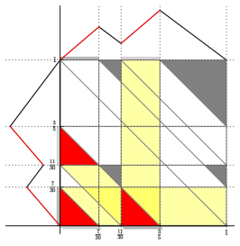
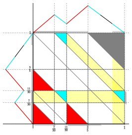
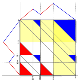
Example 6.2.

Figure 6 shows the computation for $\pi=$ gj_2_slope(3/5,1/3) step by step, where colors indicate membership to connected covered components. In Figure 6–(1), the additive face $F_{1}$ with $p_{1}(F_{1})=[\frac{11}{30},\frac{3}{5}]$, $p_{2}(F_{1})=[0,\frac{7}{30}]$ and $p_{3}(F_{1})=[\frac{11}{30},\frac{3}{5}]$ is considered. Its three projections (indicated by yellow strips on $\Delta\mathcal{P}$) are directly covered (indicated by red color on the function graphs), and they form the connected covered component $\mathcal{C}_{1}=[0,\frac{7}{30}]\cup[\frac{11}{30},\frac{3}{5}]$. In Figure 6–(2), the connected covered component $\mathcal{C}_{2}=[\frac{7}{30},\frac{11}{30}]\cup[\frac{13}{15},1]$ (with light blue color) is formed by considering the additive face $F_{2}=F([\frac{13}{15},1],[\frac{7}{30},\frac{11}{30}],[\frac{13}{15},1])$. In Figure 6–(3), the additive face $F_{3}$ with $p_{1}(F_{3})=p_{2}(F_{3})=p_{3}(F_{3})\bmod 1=[\frac{3}{5},1]$ is considered, and the connected covered component $\mathcal{C}_{3}=[\frac{3}{5},1]$ is formed. Since $\mathcal{C}_{3}$ and $\mathcal{C}_{2}$ overlap, they are merged into one large connected component $\mathcal{C}_{\mathrm{blue}}=\mathcal{C}_{2}\cup\mathcal{C}_{3}$. Therefore, all intervals are covered, and the connected components are $\mathcal{C}_{\mathrm{red}}=[0,\frac{7}{30}]\cup[\frac{11}{30},\frac{3}{5}]$ and $\mathcal{C}_{\mathrm{blue}}=[\frac{7}{30},\frac{11}{30}]\cup[\frac{3}{5},1]$.

In phase two, the program computes indirectly covered intervals and merges connected covered components according to Theorem 6.2, using one-dimensional additive faces of $\Delta\mathcal{P}$, until no further change is possible. We explain this process by the example below.

Figure 7: Compute the (directly and indirectly) covered intervals for $\pi=$ hildebrand_discont_3_slope_1()

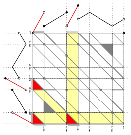
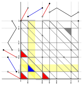
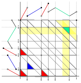
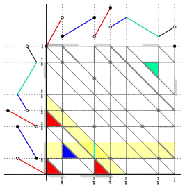
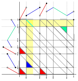
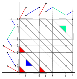
Example 6.2.

Figure 7 illustrates the computation of connected covered components for the discontinuous function $\pi$ = hildebrand_discont_3_slope_1(). In Figure 7–(1) to (3), the directly covered intervals are computed. They form the connected components $\mathcal{C}_{\mathrm{red}}=(0,\tfrac{1}{8})\cup(\tfrac{3}{8},\tfrac{1}{2}),\mathcal{C}_{\mathrm{blue}}=(\tfrac{1}{8},\tfrac{1}{4})\cup(\tfrac{1}{4},\tfrac{3}{8})$ and $\mathcal{C}_{\mathrm{green}}=(\tfrac{5}{8},\tfrac{3}{4})\cup(\tfrac{3}{4},\tfrac{7}{8})$. In Figure 7–(4), the (light blue) vertical additive edge $F(\{\frac{3}{8}\},[\frac{1}{8},\frac{1}{4}],[\frac{1}{2},\frac{5}{8}])$ is considered. Its projections $\operatorname{int}(p_{2}(F))=(\frac{1}{8},\frac{1}{4})$ and $\operatorname{int}(p_{3}(F))=(\frac{1}{2},\frac{5}{8})$ are connected through a translation. Since the interval $(\frac{1}{8},\frac{1}{4})$ was covered in the second sub-figure (as indicated by blue color), the other interval $(\frac{1}{2},\frac{5}{8})$ which was previously uncovered (as indicated by black color in Figure 7–(3)), becomes (indirectly) covered (as indicated by blue color in Figure 7–(4)). Therefore, the connected covered component $\mathcal{C}_{\mathrm{blue}}$ grows to $(\tfrac{1}{8},\tfrac{1}{4})\cup(\tfrac{1}{4},\tfrac{3}{8})\cup(\tfrac{1}{2},\tfrac{5}{8})$. In Figure 7–(5), the (light blue) diagonal additive edge $F([\frac{1}{8},\frac{1}{4}],[\frac{7}{8},1],\{\frac{9}{8}\})$ is considered, and the interval $(\tfrac{7}{8},1)$ is indirectly covered (as indicated by blue color). This concludes the computation of the connected covered components of $\pi$. They are $\mathcal{C}_{\mathrm{red}}=(0,\tfrac{1}{8})\cup(\tfrac{3}{8},\tfrac{1}{2}),\mathcal{C}_{\mathrm{blue}}=(\tfrac{1}{8},\tfrac{1}{4})\cup(\tfrac{1}{4},\tfrac{3}{8})\cup(\tfrac{1}{2},\tfrac{5}{8})\cup(\tfrac{7}{8},1)$ and $\mathcal{C}_{\mathrm{green}}=(\tfrac{5}{8},\tfrac{3}{4})\cup(\tfrac{3}{4},\tfrac{7}{8})$.

The computation of connected components of covered intervals terminates in a finite number of steps for a piecewise linear function $\pi$ with rational breakpoints. For functions with irrational breakpoints, the finiteness of the procedure remains an open question.

7 Extremality test

The command extremality_test($\pi$) implements a grid-free generalization of the automatic extremality test from [3], which is suitable also for piecewise linear functions with rational breakpoints that have huge denominators. Its support for functions with algebraic irrational breakpoints such as bhk_irrational [3, section 5] will be described in the papers [21, 17].

Given a $\mathbb{Z}$-periodic piecewise linear function $\pi$ with rational breakpoints, extremality_test($\pi$) first checks whether the conditions for minimality are satisfied, by calling minimality_test($\pi$). If $\pi$ is not minimal valid, then extremality_test($\pi$) returns False. Otherwise it proceeds, using the following theorem.

Theorem 7.1 (rephrased from [3, Lemma 4.8]).

Let $\pi$ be a piecewise linear minimal valid function with rational breakpoints. If $\pi$ is an extreme function, then the union of closures of the covered intervals of $\pi$ is equal to the whole interval $[0,1]$.

Assume that the function $\pi$ is minimal valid. The command extremality_test($\pi$) first checks whether the whole interval $[0,1]$ is covered by the union of closures of the connected covered components returned by generate_covered_intervals($\pi$). If there is an uncovered interval, then, assuming that $\pi$ be a piecewise linear function with rational breakpoints, the extremality test returns False, which is justified by Theorem 7.1. Our code also constructs an effective perturbation $\tilde{\pi}$ in this case. However, we defer an explanation of the construction of this “equivariant” [3] perturbation, as well the discussion of the case of functions with irrational breakpoints, to the paper [17].

In the following, we assume that there is no uncovered interval. Let $\mathcal{C}_{1},\mathcal{C}_{2},\dots,\mathcal{C}_{k}$ be the connected covered components of $\pi$. Let $\tilde{\pi}\in\tilde{\Pi}^{\pi}(\mathbb{R},\mathbb{Z})$ be an effective perturbation function. Then $\tilde{\pi}$ is affine linear with the same slope, say $s_{i}$, on the $i$-th connected covered component $\mathcal{C}_{i}$ for $i=1,2,\dots,k$. We also assume that $\pi$ is at least one-sided continuous at the origin. Then by 6.2, the perturbation $\tilde{\pi}$ can only be discontinuous at the points where $\pi$ is discontinuous. Let the variables $d_{j}$ ($j=1,2,\dots,m)$ denote the changes of the value of $\tilde{\pi}$ at the $m$ discontinuity points of $\pi$. In other words, the variables $d_{j}$ denote jumps $\tilde{\pi}(x)-\tilde{\pi}(x^{-})$ when $\pi$ is discontinuous at $x$ on the left, or $\tilde{\pi}(x^{+})-\tilde{\pi}(x)$ when $\pi$ is discontinuous at $x$ on the right, where $\tilde{\pi}(x^{-})$ and $\tilde{\pi}(x^{+})$ are well defined by 6.2. Since $\bigcup_{i=1}^{k}\operatorname{cl}(\mathcal{C}_{i})=[0,1]$, we have that $\tilde{\pi}$ is a piecewise linear function with breakpoints in $\{x_{0},x_{1},\dots,x_{n}\}$, which can be considered as a symbolic function over the slope parameters $s_{i}$ ($i=1,2,\dots,k$) and jump parameters $d_{j}$ ($j=1,2,\dots,m$). In fact for any $x\in[0,1]$, the value $\tilde{\pi}(x)$ is linearly determined by the variables $s_{i}$ and $d_{j}$. We can define a vector-valued piecewise linear function $g\colon[0,1]\to\mathbb{R}^{k+m}$, so that $\tilde{\pi}(x)=g(x)\cdot(s_{1},s_{2},\dots,s_{k},d_{1},d_{2},\dots,d_{m})$. This function $g$ can be set up using the command generate_symbolic in our code.

The perturbation $\tilde{\pi}$ satisfies that $\tilde{\pi}(0)=\tilde{\pi}(f)=\tilde{\pi}(1)=0$, and all the additivity relations (including additivity-in-the-limit) that $\pi$ has, by 6.0. Therefore, we have a system of linear equations for the variables $(s_{1},s_{2},\dots,s_{k},d_{1},d_{2},\dots,d_{m})$, which admits a trivial solution $(0,0,\dots,0)$. By [3, Theorem 4.11], we know that $\pi$ is an extreme function if and only if $(0,0,\dots,0)$ is the unique solution to this system. The command extremality_test($\pi$) solves the above finite-dimensional linear system using linear algebra. It returns True if the solution space has dimension $0$ or False otherwise.

Example 7.1.

Let $\pi=\texttt{hildebrand\char 95\relax\allowbreak discont\char 95\relax\allowbreak 3\char 95\relax\allowbreak slope\char 95\relax\allowbreak 1()}$ with $f=\frac{1}{2}$. As computed in the 6.2, $\pi$ has three connected covered components $\mathcal{C}_{1}=(0,\tfrac{1}{8})\cup(\tfrac{3}{8},\tfrac{1}{2}),\mathcal{C}_{2}=(\tfrac{1}{8},\tfrac{1}{4})\cup(\tfrac{1}{4},\tfrac{3}{8})\cup(\tfrac{1}{2},\tfrac{5}{8})\cup(\tfrac{7}{8},1)$ and $\mathcal{C}_{3}=(\tfrac{5}{8},\tfrac{3}{4})\cup(\tfrac{3}{4},\tfrac{7}{8})$. An effective perturbation $\tilde{\pi}\in\tilde{\Pi}^{\pi}(\mathbb{R},\mathbb{Z})$ is affine linear on $\mathcal{C}_{i}$ ($i=1,2,3$). Let $s_{i}$ denote the slope value of $\tilde{\pi}$ on $\mathcal{C}_{i}$, for $i=1,2,3$. The function $\pi$ is discontinuous at the points $\frac{1}{8}^{-},\frac{3}{8}^{+},\frac{1}{2}^{+}$ and $1^{-}$. Let $d_{1}=\tilde{\pi}(\frac{1}{8})-\tilde{\pi}(\frac{1}{8}^{-})$, $d_{2}=\tilde{\pi}(\frac{1}{2}^{+})-\tilde{\pi}(\frac{1}{2})$, $d_{3}=\tilde{\pi}(\frac{3}{8}^{+})-\tilde{\pi}(\frac{3}{8})$ and $d_{4}=\tilde{\pi}(1)-\tilde{\pi}(1^{-})$. We know that $\tilde{\pi}(0)=0$, $\tilde{\pi}(f)=0$ and $\tilde{\pi}(1)=0$. Define the piecewise linear function $g\colon[0,1]\to\mathbb{R}^{7}$, such that

$$g(x)=\begin{cases}(1,0,0,0,0,0,0)x&\text{if }0\leq x<\frac{1}{8}\\ (0,1,0,0,0,0,0)x+(\frac{1}{8},-\frac{1}{8},0,1,0,0,0)&\text{if }\frac{1}{8}\leq x\leq\frac{3}{8}\\ (1,0,0,0,0,0,0)x-(\frac{1}{4},-\frac{1}{4},0,-1,-1,0,0)&\text{if }\frac{3}{8}<x\leq\frac{1}{2}\\ (0,1,0,0,0,0,0)x+(\frac{1}{4},-\frac{1}{4},0,1,1,1,0)&\text{if }\frac{1}{2}<x\leq\frac{5}{8}\\ (0,0,1,0,0,0,0)x+(\frac{1}{4},\frac{3}{8},-\frac{5}{8},1,1,1,0)&\text{if }\frac{5}{8}<x\leq\frac{7}{8}\\ (0,1,0,0,0,0,0)x+(\frac{1}{4},-\frac{1}{2},\frac{1}{4},1,1,1,0)&\text{if }\frac{7}{8}<x<1\\ (\frac{1}{4},\frac{1}{2},\frac{1}{4},1,1,1,1)&\text{if }x=1.\end{cases}$$

This function $g$ can be obtained by calling

h = hildebrand_discont_3_slope_1(); components = generate_covered_intervals(h); g = generate_symbolic(h, components, field=QQ). Ψ

Then $\pi(x)=g(x)\cdot(s_{1},s_{2},s_{3},d_{1},d_{2},d_{3},d_{4})$, for $0\leq x\leq 1$. It follows from the symmetry condition that $d_{1}=d_{3}$ and $d_{2}=d_{4}$. By considering the additive limiting cones on the diagram of $\Delta\mathcal{P}$ (see Figure 5–left) and by 6.0, we obtain that $\tilde{\pi}(\frac{1}{8}^{+})+\tilde{\pi}(\frac{1}{2}^{+})=\tilde{\pi}(\frac{5}{8}^{+})$, $\tilde{\pi}(\frac{7}{8}^{-})+\tilde{\pi}(\frac{7}{8}^{-})=\tilde{\pi}(\frac{7}{4}^{-})$ and $\tilde{\pi}(0^{-})+\tilde{\pi}(\frac{1}{8}^{+})=\tilde{\pi}(\frac{1}{8}^{-})$. These additivity relations, along with $\tilde{\pi}(f)=0$ and $\tilde{\pi}(1)=0$, imply the linear system

$$\begin{pmatrix}\tfrac{1}{4}&\tfrac{1}{4}&0&1&1&0&0\\ \tfrac{1}{4}&\tfrac{1}{2}&\tfrac{1}{4}&1&1&1&1\\ 0&0&0&1&0&-1&0\\ 0&0&0&0&1&0&-1\\ \tfrac{1}{8}&-\tfrac{1}{8}&0&1&0&0&0\\ \tfrac{1}{4}&\tfrac{3}{8}&\tfrac{3}{8}&1&1&1&0\\ \tfrac{1}{4}&\tfrac{1}{2}&\tfrac{1}{4}&2&1&1&0\end{pmatrix}\begin{pmatrix}s_{1}\\ s_{2}\\ s_{3}\\ d_{1}\\ d_{2}\\ d_{3}\\ d_{4}\end{pmatrix}=0.$$

The above system has the unique solution $s_{1}=s_{2}=s_{3}=d_{1}=d_{2}=d_{3}=d_{4}=0$. Therefore, $\pi$ is an extreme function.

Table 3: A sample Sage session on the extremality test

Ψ## First we load a function and store it in variable h. Ψ## We start with the easiest function, the GMIC. Ψsage: h = gmic() ΨINFO: 2016-08-08 16:51:31,048 Rational case. Ψ Ψ## Test its extremality; this will create informative output and plots Ψsage: extremality_test(h, show_plots=True) ΨINFO: 2016-08-08 16:54:22,014 pi(0) = 0 ΨINFO: 2016-08-08 16:54:22,016 pi is subadditive. ΨINFO: 2016-08-08 16:54:22,016 pi is symmetric. ΨINFO: 2016-08-08 16:54:22,018 Thus pi is minimal. ΨINFO: 2016-08-08 16:54:22,018 Plotting 2d diagram... ΨINFO: 2016-08-08 16:54:22,018 Computing maximal additive faces... ΨINFO: 2016-08-08 16:54:22,022 Computing maximal additive faces... done ΨLaunched png viewer for Graphics object consisting of 25 graphics primitives ΨINFO: 2016-08-08 16:54:22,526 Plotting 2d diagram... done ΨINFO: 2016-08-08 16:54:22,526 Computing covered intervals... ΨINFO: 2016-08-08 16:54:22,527 Computing covered intervals... done ΨINFO: 2016-08-08 16:54:22,527 Plotting covered intervals... ΨLaunched png viewer for Graphics object consisting of 2 graphics primitives ΨINFO: 2016-08-08 16:54:22,985 Plotting covered intervals... done ΨINFO: 2016-08-08 16:54:22,986 All intervals are covered (or connected-to-covered). 2 components. ΨINFO: 2016-08-08 16:54:23,035 Finite dimensional test: Solution space has dimension 0 ΨINFO: 2016-08-08 16:54:23,035 Thus the function is extreme. Ψ Ψ## The docstring tells us that we can set the ‘f’ value using an optional argument. Ψsage: h = gmic(1/5) ΨINFO: 2016-08-08 16:55:59,440 Rational case. Ψ## Of course, we know it will still be extreme; but let’s test it to Ψ## see all the informative graphs. Ψsage: extremality_test(h, show_plots=True) Ψ[...] ΨTrue Ψ## Let’s try a different function from the compendium. Ψ## We change the parameters a little bit, so that they do NOT satisfy the known Ψ## sufficient conditions from the literature about this class of functions. Ψsage: h = drlm_backward_3_slope(f=1/12, bkpt=4/12) ΨINFO: 2016-08-08 17:03:20,438 Conditions for extremality are NOT satisfied. ΨINFO: 2016-08-08 17:03:20,439 Rational case. Ψ Ψ## Let’s run the extremality test. Ψsage: extremality_test(h, show_plots=True) Ψ[...] ΨINFO: 2016-08-08 17:03:44,796 Thus pi is minimal. Ψ[...] ΨINFO: 2016-08-08 17:03:46,417 Uncovered intervals: ([[5/12, 2/3]],) Ψ[...] ΨINFO: 2016-08-08 17:03:49,544 Plotting perturbation... done ΨINFO: 2016-08-08 17:03:49,545 Thus the function is NOT extreme. ΨFalse Ψ## Indeed, it’s not extreme. Ψ## We see a perturbation in magenta and the two perturbed functions in blue and red, Ψ## whose average is the original function (black). Ψ Ψ## Here’s the Gomory fractional cut. Ψsage: h = gomory_fractional() Ψ## It is not even minimal: Ψsage: minimality_test(h, True) ΨINFO: 2016-08-08 17:06:33,647 pi(0) = 0 ΨINFO: 2016-08-08 17:06:33,648 pi is not minimal because it does not stay in the range of [0, 1]. ΨFalse Ψ Ψ## There’s many more functions to explore. Use the Tab key on the next line to see a collection of those functions. Ψsage: extreme_functions.[tab] Ψ

8 Transformations of piecewise linear functions

The Python module named procedures gives access to the “procedures” that can transform extreme functions. These procedures include the transformations between functions for finite and infinite group problems that we will discuss in section 9, and other well-known transformations; see [4, Table 5]. For instance, we have:

multiplicative_homomorphism

constructs the function $x\mapsto\pi(\lambda x)$ for a given piecewise linear function $\pi$, where $\lambda$ is a nonzero integer; see [26, sections 19.4.1, 19.5.2.1]. (The use of the word “multiplicative homomorphism” for this operation comes from [26].)

automorphism

is a special case of the above, where $\lambda$ is $\pm 1$, so that $x\mapsto\lambda x$ is an automorphism of the group $\mathbb{R}/\mathbb{Z}$. If a different factor $\lambda$ is provided, an error is signalled. Since $\lambda=-1$ gives the only nontrivial automorphism, $x\mapsto\pi(-x)$, this is the default. See [19] for a discussion.

projected_sequential_merge

performs the one-dimensional projected sequential merge, with operator $\lozenge_{n}^{1}\,(\texttt{gmic})$, on an extreme function $\pi$; see [10].

Newly discovered procedures since the publication of [4] have been implemented as well.

symmetric_2_slope_fill_in

returns an extreme 2-slope function that approximates the given continuous minimal valid function $\pi$ with infinity norm distance less than $\epsilon$, under the assumption that $f$ is a rational number; see [7].

symmetric_2_slope_fill_in_irrational

is a variant, proposed by the third author, Yuan Zhou (2015, unpublished), of the above procedure symmetric_2_slope_fill_in, which removes the assumption $f\in\mathbb{Q}$.

9 Functionality for the finite (cyclic) group relaxation model

Let $q$ be a positive integer and let $f\in\frac{1}{q}\mathbb{Z}$. A discrete function $\pi|_{\frac{1}{q}\mathbb{Z}}\colon\frac{1}{q}\mathbb{Z}\to\mathbb{R}_{+}$ is minimal valid for Gomory–Johnson’s finite (cyclic) group relaxation model if and only if $\pi|_{\frac{1}{q}\mathbb{Z}}$ is $\mathbb{Z}$-periodic, subadditive, $\pi|_{\frac{1}{q}\mathbb{Z}}(0)=0$, and satisfies the symmetry condition. A minimal valid function $\pi|_{\frac{1}{q}\mathbb{Z}}$ is extreme if it is not a proper convex combination of other minimal valid functions.

In our code, a $\mathbb{Z}$-periodic discrete function $\pi|_{\frac{1}{q}\mathbb{Z}}$ can be set up using the Python function named discrete_function_from_points_and_values(points, values), given two finite lists points and values which represent the domain of $\pi|_{\frac{1}{q}\mathbb{Z}}$ restricted to the interval $[0,1]$ and the function values at these points, respectively.

Another important way to obtain a discrete function $\pi|_{\frac{1}{q}\mathbb{Z}}$ is to restrict a piecewise linear function $\pi$ for the infinite group problem to the cyclic group of given order $q$, by calling the procedure restrict_to_finite_group. Conversely, the procedure interpolate_to_infinite_group provides the piecewise linear interpolation $\pi$ of a given discrete function $\pi|_{\frac{1}{q}\mathbb{Z}}$.

The functionalities plot_2d_diagram, minimality_test and extremality_test that we described above also work for $\pi|_{\frac{1}{q}\mathbb{Z}}$ in the finite group model.

The transformations (procedures) multiplicative_homomorphism and automorphism described in section 8 are also available for the finite group case. The latter is more interesting in the finite group case, because the cyclic group $\frac{1}{q}\mathbb{Z}/\mathbb{Z}$ has more nontrivial automorphisms. Indeed, studying the action of the automorphisms was a major focus of Gomory’s original paper [13]. The given factor $\lambda$ must be an integer coprime with the group order $q$; see [26, section 19.5.2.1].

See Table 4 for a sample Sage session on discrete functions for the finite group problem and the related transformations.

Table 4: A sample Sage session on discrete functions for the finite group problem.

Ψ## We load the GMIC function with f=4/5, and store it in variable h. Ψsage: h = gmic(f=4/5) ΨINFO: 2016-08-08 17:23:05,206 Rational case. Ψ Ψ## We can restrict to a finite group problem. Ψsage: restrict_to_finite_group? ΨSignature: restrict_to_finite_group(function, f=None, oversampling=None, order=None) ΨDocstring: ΨRestrict the given function to the cyclic group of given order. Ψ Ψ If order is not given, it defaults to the group generated by the Ψ breakpoints of function and f if these data are rational. However, Ψ if oversampling is given, it must be a positive integer; then the Ψ group generated by the breakpoints of function and f will be Ψ refined by that factor. Ψ Ψ If f is not provided, uses the one found by find_f. Ψ Ψ Assume in the following that f and all breakpoints of function lie Ψ in the cyclic group and that function is continuous. Ψ Ψ Then the restriction is minimal valid if and only if function is minimal valid. Ψ The restriction is extreme if function is extreme. Ψ Ψ If, in addition oversampling >= 3, then the following holds: The Ψ restriction is extreme if and only if function is extreme. This is Ψ Theorem 1.5 in [IR2]. Ψ Ψ This oversampling factor of 3 is best possible, as demonstrated by Ψ function kzh_2q_example_1 from [KZh2015a]. Ψ [...] Ψsage: hr = restrict_to_finite_group(h) ΨINFO: 2016-08-08 17:26:36,047 Rational breakpoints and f; Ψusing group generated by them, (1/5)Z Ψ Ψ## This function can be set up by providing the breakpoints and the values. Ψsage: discrete_function_from_points_and_values(points=[0, 1/5, 2/5, 3/5, 4/5, 1], Ψ values=[0, 1/4, 1/2, 3/4, 1, 0]) == hr ΨINFO: 2016-08-8 17:26:37,190 Rational case. ΨTrue Ψ## The restricted function is extreme for the finite group problem. Ψsage: extremality_test(hr) ΨINFO: 2016-08-8 17:26:38,121 pi(0) = 0 ΨINFO: 2016-08-8 17:26:38,123 pi is subadditive. ΨINFO: 2016-08-8 17:26:38,123 pi is symmetric. ΨINFO: 2016-08-8 17:26:38,124 Thus pi is minimal. ΨINFO: 2016-08-8 17:26:38,124 Rational breakpoints and f; Ψusing group generated by them, (1/5)Z ΨINFO: 2016-08-8 17:26:38,158 Solution space has dimension 0 ΨINFO: 2016-08-8 17:26:38,158 Thus the function is extreme. ΨTrue Ψ Ψ## For the finite group problems, automorphisms are interesting! Ψsage: ha = automorphism(hr, 2) ΨINFO: 2016-08-08 17:26:41,100 Rational breakpoints and f; Ψusing group generated by them, (1/5)Z Ψ Ψ## We can interpolate to get a function for the infinite group problem. Ψsage: hi = interpolate_to_infinite_group(ha) Ψ

10 Documentation and test suite

Following the standard conventions of Sage, the documentation strings contain usage examples with their expected output. If Sage is invoked as

sage -t $\langle\mathit{filename}\rangle$.sage,

these examples are run and their results are compared to the expected results; if the results differ, this is reported as a unit test failure. This helps to ensure the consistency and correctness of the algorithms and of the compendium of extreme functions as we continue developing the software. The command make check runs the tests for all files of our software.

A substantial part of our software is concerned with plotting certain diagrams. Our code also contains a testsuite of diagrams that have been published in the survey [4, 5] and in several research papers to ensure that these diagrams can still be reproduced with new versions of our software. The testsuite, invoked by make check-graphics, produces a multi-page PDF file which needs to be compared with a “good” copy of the PDF file by visual inspection.

Finally, demo.sage demonstrates further functionality and the use of the help system.

Funding

The first author’s contribution was done during a Research Experience for Undergraduates at the University of California, Davis. He was partially supported by the National Science Foundation through grant DMS-0636297 (VIGRE). All authors were partially supported by the National Science Foundation through grant DMS-1320051 awarded to M. Köppe. The support is gratefully acknowledged.

Appendix A Enumerating the maximal additive faces of $\Delta\mathcal{P}$ in the continuous case

In this section, we explain the algorithm that the code generate_maximal_additive_faces_continuous($\pi$) uses to enumerate the maximal additive faces for a continuous subadditive function $\pi$. For functions with many breakpoints, it pays off to avoid duplicate computations that would arise from the fact that a given lower-dimensional face $F$ of $\Delta\mathcal{P}$ has many representations as $F(I,J,K)$ with $I,J,K\in\mathcal{P}$. The algorithm considers the full-dimensional (two-dimensional) faces $F=F(I,J,K)$ of $\Delta\mathcal{P}$ in the lexicographic order on $(I,J,K)$, where $I,J,K$ are proper intervals of $\mathcal{P}$ with $I,J\subseteq[0,1]$ and $K\subseteq[0,2]$, and $I\leq J$, i.e., $I$ is to the left of $J$ on the real line. The algorithm has a fast path for discarding faces $F(I,J,K)$ that are not full-dimensional. Lower-dimensional additive faces will be considered as subfaces of full-dimensional faces as follows. The algorithm distinguishes the following four cases, depending on the number of additive vertices that each full-dimensional $F$ has.

1. If $F$ has no additive vertex, then $F$ does not contain any maximal additive face of $\Delta\mathcal{P}$ (nothing is green in $F$). No recording is needed for this face $F$.

2. If $F$ has only one additive vertex, denoted by $(x,y)$, then this vertex could either be a maximal additive face, or it could be a subface of a maximal additive face that is not a subface of $F$. We maintain a hashed set of all vertices of maximal additive faces that have already been recorded during the algorithm. We only process $(x,y)$ when $F$ is the last two-dimensional face $F(I,J,K)$ in the lexicographic order on $(I,J,K)$ that contains $(x,y)$. This condition is easy to check; see Figure 8 for an illustration of the cases.

   (a)  (b)  (c) 

   Figure 8: An additive vertex $(x,y)$ is processed when it arises as a subface of the last two-dimensional face $F=F(I,J,K)$ in the lexicographic order on $(I,J,K)$ that contains $(x,y)$. (a) $x$ and $y$ are the left endpoints of $I$ and $J$; (b) $x$ and $x+y$ are the left endpoints of $I$ and $K$; (c) $y$ and $x+y$ are the left endpoints of $J$ and $K$.

   In that case, we record $(x,y)$ as a maximal additive face of $\Delta\mathcal{P}$ when $(x,y)$ is not a vertex of a maximal additive face that has already been recorded.

3. If $F$ has exactly two additive vertices, then they form an additive edge $E$. It cannot lie in the interior of $F$, since otherwise $\Delta\pi=0$ holds over all $F$, contradicting the assumption that only two vertices of the two-dimensional face $F$ are additive. Therefore, this additive edge $E$ is a subface of $F$, and hence a one-dimensional additive face of $\Delta\mathcal{P}$. Again we only process $E$ when $F$ is the last two-dimensional face $F(I,J,K)$ in the lexicographic order on $(I,J,K)$ that contains $E$. (There is only one other face $F^{\prime}$ containing $E$; see Figure 9.) In that case, we record $E$ if $F^{\prime}$ was not recorded as an additive face.

   Figure 9: An additive edge $E=F^{\prime}\cap F$ with $F^{\prime}<F$ in the lexicographic order on $(I,J,K)$ is processed when it arises as a subface of $F$

4. If $F$ has more than $2$ additive vertices, then $\Delta\pi=0$ holds over all $F$. The face $F$ is recorded as a maximal additive face of $\Delta\mathcal{P}$.

References

- [1] SageMath Trac development server. URL: https://trac.sagemath.org.
- [2] C. Alves, F. Clautiaux, J.V. de Carvalho, and J. Rietz, Dual-Feasible Functions for Integer Programming and Combinatorial Optimization: Basics, Extensions and Applications, EURO Advanced Tutorials on Operational Research, Springer, 2016. doi:10.1007/978-3-319-27604-5.
- [3] A. Basu, R. Hildebrand, and M. Köppe, Equivariant perturbation in Gomory and Johnson’s infinite group problem. I. The one-dimensional case, Mathematics of Operations Research 40 (2014), pp. 105–129. doi:10.1287/moor.2014.0660.
- [4] A. Basu, R. Hildebrand, and M. Köppe, Light on the infinite group relaxation I: foundations and taxonomy, 4OR 14 (2016), pp. 1–40. doi:10.1007/s10288-015-0292-9.
- [5] A. Basu, R. Hildebrand, and M. Köppe, Light on the infinite group relaxation II: sufficient conditions for extremality, sequences, and algorithms, 4OR 14 (2016), pp. 107–131. doi:10.1007/s10288-015-0293-8.
- [6] A. Basu, R. Hildebrand, and M. Köppe, Equivariant perturbation in Gomory and Johnson’s infinite group problem—III: Foundations for the -dimensional case with applications to , Mathematical Programming 163 (2017), pp. 301–358. doi:10.1007/s10107-016-1064-9.
- [7] A. Basu, R. Hildebrand, and M. Molinaro, Minimal cut-generating functions are nearly extreme, in Integer Programming and Combinatorial Optimization: 18th International Conference, IPCO 2016, Liège, Belgium, June 1–3, 2016, Proceedings, Q. Louveaux and M. Skutella, eds., Springer International Publishing, Cham, 2016, pp. 202–213. doi:10.1007/978-3-319-33461-5_17.
- [8] A. Basu, M. Conforti, M. Di Summa, and J. Paat, Extreme functions with an arbitrary number of slopes, in Integer Programming and Combinatorial Optimization: 18th International Conference, IPCO 2016, Liège, Belgium, June 1–3, 2016, Proceedings, Q. Louveaux and M. Skutella, eds., Springer International Publishing, Cham, 2016, pp. 190–201. doi:10.1007/978-3-319-33461-5_16.
- [9] M. Conforti, G. Cornuéjols, A. Daniilidis, C. Lemaréchal, and J. Malick, Cut-generating functions and S-free sets, Mathematics of Operations Research 40 (2013), pp. 253–275. doi:10.1287/moor.2014.0670.
- [10] S.S. Dey and J.P.P. Richard, Relations between facets of low- and high-dimensional group problems, Mathematical Programming 123 (2010), pp. 285–313. doi:10.1007/s10107-009-0303-8.
- [11] S.S. Dey, J.P.P. Richard, Y. Li, and L.A. Miller, On the extreme inequalities of infinite group problems, Mathematical Programming 121 (2010), pp. 145–170. doi:10.1007/s10107-008-0229-6.
- [12] R.E. Gomory, An algorithm for the mixed integer problem, Tech. Rep., DTIC Document, 1960.
- [13] R.E. Gomory, Some polyhedra related to combinatorial problems, Linear Algebra and its Applications 2 (1969), pp. 451–558.
- [14] R.E. Gomory and E.L. Johnson, Some continuous functions related to corner polyhedra, I, Mathematical Programming 3 (1972), pp. 23–85. doi:10.1007/BF01584976.
- [15] R.E. Gomory and E.L. Johnson, Some continuous functions related to corner polyhedra, II, Mathematical Programming 3 (1972), pp. 359–389. doi:10.1007/BF01585008.
- [16] R.E. Gomory and E.L. Johnson, T-space and cutting planes, Mathematical Programming 96 (2003), pp. 341–375. doi:10.1007/s10107-003-0389-3.
- [17] R. Hildebrand, M. Köppe, and Y. Zhou, Equivariant perturbation in Gomory and Johnson’s infinite group problem. VII. Grid-free extremality test—general algorithm and implementation, 2016. manuscript.
- [18] C.Y. Hong, M. Köppe, and Y. Zhou, SageMath program for computation and experimentation with the -dimensional Gomory–Johnson infinite group problem (2014–2017). URL: https://github.com/mkoeppe/infinite-group-relaxation-code.
- [19] E.L. Johnson, On the group problem for mixed integer programming, Mathematical Programming Study 2 (1974), pp. 137–179.
- [20] M. Köppe and Y. Zhou, An electronic compendium of extreme functions for the Gomory–Johnson infinite group problem, Operations Research Letters 43 (2015), pp. 438–444. doi:10.1016/j.orl.2015.06.004.
- [21] M. Köppe and Y. Zhou, Equivariant perturbation in Gomory and Johnson’s infinite group problem. VI. The curious case of two-sided discontinuous functions, eprint arXiv:1605.03975 [math.OC] (2016).
- [22] M. Köppe and Y. Zhou, New computer-based search strategies for extreme functions of the Gomory–Johnson infinite group problem, Mathematical Programming Computation (2016), pp. 1–51. doi:10.1007/s12532-016-0115-9.
- [23] M. Köppe and Y. Zhou, Toward computer-assisted discovery and automated proofs of cutting plane theorems, in Combinatorial Optimization: 4th International Symposium, ISCO 2016, Vietri sul Mare, Italy, May 16–18, 2016, Revised Selected Papers, R. Cerulli, S. Fujishige, and A.R. Mahjoub, eds., Springer International Publishing, Cham, 2016, pp. 332–344. doi:10.1007/978-3-319-45587-7_29.
- [24] Q. Louveaux and L.A. Wolsey, Lifting, superadditivity, mixed integer rounding and single node flow sets revisited, Quarterly Journal of the Belgian, French and Italian Operations Research Societies 1 (2003), pp. 173–207. doi:10.1007/s10288-003-0016-4.
- [25] L.A. Miller, Y. Li, and J.P.P. Richard, New inequalities for finite and infinite group problems from approximate lifting, Naval Research Logistics (NRL) 55 (2008), pp. 172–191. doi:10.1002/nav.20275.
- [26] J.P.P. Richard and S.S. Dey, The group-theoretic approach in mixed integer programming, in 50 Years of Integer Programming 1958–2008, M. Jünger, T.M. Liebling, D. Naddef, G.L. Nemhauser, W.R. Pulleyblank, G. Reinelt, G. Rinaldi, and L.A. Wolsey, eds., Springer Berlin Heidelberg, 2010, pp. 727–801. doi:10.1007/978-3-540-68279-0_19.
- [27] J.P.P. Richard, Y. Li, and L.A. Miller, Valid inequalities for MIPs and group polyhedra from approximate liftings, Mathematical Programming 118 (2009), pp. 253–277. doi:10.1007/s10107-007-0190-9.
- [28] W.A. Stein, et al., Sage Mathematics Software (Version 7.1), The Sage Development Team (2016), http://www.sagemath.org.