Semiparametric estimation for isotropic max-stable space-time processes

Sven Buhllabel=e1 [    mark]sven.buhl@tum.de    Richard A. Davislabel=e2 [    mark]rdavis@stat.columbia.edulabel=u2 [    url]http://www.stat.columbia.edu/~rdavis    Claudia Klüppelberglabel=e3 [    mark]cklu@tum.de    Christina Steinkohllabel=e4 [    mark]christina.steinkohl@gmail.comlabel=u1 [    url]http://www.statistics.ma.tum.de Center for Mathematical Sciences and TUM Institute of Advanced Study, Technische Universität München, Boltzmannstr. 3, 85748 Garching, Germany. , Department of Statistics, Columbia University, 1255 Amsterdam Avenue, New York, NY 10027, USA. ,
Brown-Resnick process,
extremogram,
max-stable process,
regular variation,
semiparametric estimation,
space-time process,
subsampling,
mixing,
keywords:
\arxiv

1609.04967 \startlocaldefs \endlocaldefs

and

Regularly varying space-time processes have proved useful to study extremal dependence in space-time data. We propose a semiparametric estimation procedure based on a closed form expression of the extremogram to estimate parametric models of extremal dependence functions. We establish the asymptotic properties of the resulting parameter estimates and propose subsampling procedures to obtain asymptotically correct confidence intervals. A simulation study shows that the proposed procedure works well for moderate sample sizes and is robust to small departures from the underlying model. Finally, we apply this estimation procedure to fitting a max-stable process to radar rainfall measurements in a region in Florida. Complementary results and some proofs of key results are presented together with the simulation study in the supplement Buhl et al. [7].

1 Introduction

Regularly varying processes provide a useful framework for modeling extremal dependence in continuous time or space. They have been investigated in Hult and Lindskog [19, 20]. A prominent class of examples consists of max-stable processes. A key example in this paper is the max-stable Brown-Resnick process which was introduced in a time series framework in Brown and Resnick [2], in a spatial setting in Kabluchko et al. [22], and extended to a space-time setting in Davis et al. [10].

In the literature, various dependence models and estimation procedures have been proposed for extremal data. For the Brown-Resnick process with parametrized dependence structure, inference has been based on composite likelihood methods. In particular, pairwise likelihood estimation has been found useful to estimate parameters in a max-stable process. A description of this method can be found in Padoan et al. [24] for the spatial setting, and Huser and Davison [21] in a space-time setting. Asymptotic results for pairwise likelihood estimates and detailed analyses in the space-time setting for the model analysed in this paper are given in Davis et al. [11]. Unfortunately, parameter estimation using composite likelihood methods can be laborious, since the computation and subsequent optimization of the objective function is time-consuming. Also the choice of good initial values for the optimization of the composite likelihood is essential.

In this paper we introduce a new semiparametric estimation procedure for regularly varying processes which is based on the extremogram as a natural extremal analog of the correlation function for stationary processes. The extremogram was introduced in Davis and Mikosch [9] for time series (also in Fasen et al. [16]), and they show consistency and asymptotic normality of an empirical extremogram estimate under weak mixing conditions. The empirical extremogram and its asymptotic properties in a spatial setting have been investigated in Buhl and Klüppelberg [5] and Cho et al. [8]. It can serve as a useful graphical tool for assessing extremal dependence structures in spatial and space-time processes that provides clues about potential parametric models, a critical step in the model building paradigm. For example, compatibility with various assumptions such as isotropy and stationarity (see Buhl and Klüppelberg [4] and Davis et al. [11] for some examples), can be assessed by examining invariance of the empirical extremogram when computed over specially chosen subsets of the data. Ultimately, a number of families of proposed parametric models are often fitted before deciding on a particular class of models. Therefore it is of interest to be able to not only have a procedure that can compute estimates rapidly, but also to serve as a check on the efficacy of model choice. Additionally, the new estimation procedure allows one to provide parameter estimates that can be used as initial values in more refined procedures, such as composite likelihood.

Our semiparametric estimation method assumes a spatially isotropic and additively separable dependence structure for regularly varying space-time processes. We first estimate the extremogram nonparametrically by its empirical version, where we can hence separate space and time. Weighted linear regression is then applied in order to produce parameter estimates. Asymptotic normality of these semiparametric estimates requires asymptotic normality of the empirical extremogram, and we apply the CLT with mixing conditions as provided in [5]. The rate of convergence can be improved by a bias correction term, a fact which we explain in detail. The proofs of the asymptotic properties of semiparametric spatial and temporal parameter estimates are analogous, and we present the details on the spatial parameters only, referring to Buhl [3], Chapter 3, for details about the asymptotic properties of the semiparametric temporal parameter.

In a second step we establish asymptotic normality of the weighted least squares parameter estimates. When the dependence parameters have bounded support, as for the Brown-Resnick process in Section 4, constrained optimization has to be applied. Then also the limit law differs depending whether the true parameters lie on the boundary or not. Since the asymptotic covariance matrix in the normal limit is difficult to access, we apply subsampling procedures to obtain pointwise confidence intervals for the parameters.

The semiparametric estimates converge at a slower rate than the square root rate of a fully parametric procedure such as pairwise likelihood estimation. However, it is known that likelihood-based estimates may be inefficient and even not consistent if the model is slightly misspecified. The semiparametric estimates, however, are often unaffected by slight deviations in the model. This is proved in Section 9 and illustrated in Section 10 of the supplement [7], where data are generated from a Brown-Resnick process, but with observational noise. The semiparametric estimates clearly outperform pairwise likelihood estimates in this case. On the other hand, the semiparametric estimates perform admirably well relative to the pairwise likelihood estimates when the underlying process is in fact a Brown-Resnick process.

Our paper is organized as follows. Section 2 defines regularly varying processes in space and time and their extremogram. Based on gridded data, the nonparametric extremogram estimation is derived and used for parametric model fitting. Asymptotic normality of the parameter estimates is established in Section 3. Section 3.1 is dedicated to the asymptotic normality of the empirical extremogram; and Section 3.2 deals with the asymptotic properties of the parameter estimates. The subsampling procedure – as well as results and proofs for our setting – is given in Section 7 of the supplement [7]. In Section 4 we apply the semiparametric method to the Brown-Resnick process and verify the required conditions. Here we also calculate the bias corrected estimator. We test our new semiparametric estimation procedure in a simulation study presented in the supplement [7] and compare it to pairwise likelihood estimation, both when applied to data generated by a Brown-Resnick process and when the data are affected by observational noise. In the latter, our procedure produces estimates with less bias than those based on pairwise likelihood (see Section 10 of the supplement [7]). The paper concludes with an analysis of daily rainfall maxima in a region in Florida in Section 5, where we also compare the semiparametric estimates with previously obtained pairwise likelihood estimates. The supplement [7] contains four sections, on subsampling, on α𝛼{\alpha}-mixing of the Brown-Resnick process, a robustness result for the bias corrected estimator, and a simulation study.

2 Model description and semiparametric estimates

In this paper we consider strictly stationary regularly varying processes in space and time {η(𝒔,t):𝒔d1,t[0,)}conditional-set𝜂𝒔𝑡formulae-sequence𝒔superscript𝑑1𝑡0\{\eta(\boldsymbol{s},t):\boldsymbol{s}\in\mathbb{R}^{d-1},t\in[0,\infty)\} for d𝑑d\in\mathbb{N}, where all finite-dimensional distributions are regularly varying (cf. Hult and Lindskog [20] for definitions and results in a general framework and Resnick [25] for details about multivariate regular variation). Throughout, f(n)g(n)similar-to𝑓𝑛𝑔𝑛f(n)\sim g(n) means that limnf(n)g(n)=1subscript𝑛𝑓𝑛𝑔𝑛1\lim_{n\to\infty}\frac{f(n)}{g(n)}=1. As a prerequisite, we define for every finite set d1×[0,)superscript𝑑10\mathcal{I}\subset\mathbb{R}^{d-1}\times[0,\infty) with cardinality |||\mathcal{I}| the vector

η:=(η(𝒔,t):(𝒔,t)).\eta_{\mathcal{I}}:=(\eta(\boldsymbol{s},t):(\boldsymbol{s},t)\in\mathcal{I}){}^{{}^{\intercal}}.

Let furthermore \|\cdot\| be the Euclidean norm on d1superscript𝑑1\mathbb{R}^{d-1}.

Definition 2.1 (Regularly varying stochastic process).

A strictly stationary stochastic space-time process {η(𝒔,t):(𝒔,t)d1×[0,)}conditional-set𝜂𝒔𝑡𝒔𝑡superscript𝑑10\{\eta(\boldsymbol{s},t):(\boldsymbol{s},t)\in\mathbb{R}^{d-1}\times[0,\infty)\} is called regularly varying, if there exists some normalizing sequence 0<an0subscript𝑎𝑛0<a_{n}\to\infty such that (|η(𝟎,0)|>an)ndsimilar-to𝜂00subscript𝑎𝑛superscript𝑛𝑑\mathbb{P}(|\eta(\boldsymbol{0},0)|>a_{n})\sim n^{-d} as n𝑛n\to\infty, and if for every finite set d1×[0,)superscript𝑑10\mathcal{I}\subset\mathbb{R}^{d-1}\times[0,\infty),

nd(ηan)vμ(),n,formulae-sequencesuperscript𝑣superscript𝑛𝑑subscript𝜂subscript𝑎𝑛subscript𝜇𝑛\displaystyle n^{d}\mathbb{P}\Big{(}\frac{\eta_{\mathcal{I}}}{a_{n}}\in\cdot\Big{)}\stackrel{{\scriptstyle v}}{{\rightarrow}}\mu_{\mathcal{I}}(\cdot),\quad n\rightarrow\infty, (2.1)

for some non-null Radon measure μsubscript𝜇\mu_{\mathcal{I}} on the Borel sets in ¯||\{𝟎}\superscript¯0\overline{\mathbb{R}}^{|\mathcal{I}|}\backslash\{\boldsymbol{0}\}. In that case,

μ(xC)=xβμ(C),x>0,formulae-sequencesubscript𝜇𝑥𝐶superscript𝑥𝛽subscript𝜇𝐶𝑥0\mu_{\mathcal{I}}(xC)=x^{-\beta}\mu_{\mathcal{I}}(C),\quad x>0,

for every Borel set C𝐶C in ¯||\{𝟎}\superscript¯0\overline{\mathbb{R}}^{|\mathcal{I}|}\backslash\{\boldsymbol{0}\}. The notation vsuperscript𝑣\stackrel{{\scriptstyle v}}{{\rightarrow}} stands for vague convergence, and β>0𝛽0\beta>0 is called the index of regular variation.

For every (𝒔,t)d1×[0,)𝒔𝑡superscript𝑑10(\boldsymbol{s},t)\in\mathbb{R}^{d-1}\times[0,\infty) and ={(𝒔,t)}𝒔𝑡\mathcal{I}=\{(\boldsymbol{s},t)\} we set μ{(𝒔,t)}()=μ{(𝟎,0)}()=:μ(),\mu_{\{(\boldsymbol{s},t)\}}(\cdot)=\mu_{\{(\boldsymbol{0},0)\}}(\cdot)=:\mu(\cdot), which is justified by stationarity. Throughout we furthermore consider the space-time process {η(𝒔,t):(𝒔,t)d1×[0,)}conditional-set𝜂𝒔𝑡𝒔𝑡superscript𝑑10\{\eta(\boldsymbol{s},t):(\boldsymbol{s},t)\in\mathbb{R}^{d-1}\times[0,\infty)\} to be spatially isotropic. Together with the assumption of strict stationarity, this means that extremal dependence between two space-time points (𝒔1,t1)subscript𝒔1subscript𝑡1(\boldsymbol{s}_{1},t_{1}) and (𝒔2,t2)subscript𝒔2subscript𝑡2(\boldsymbol{s}_{2},t_{2}) is only driven by the spatial and temporal lags v:=𝒔1𝒔2assign𝑣normsubscript𝒔1subscript𝒔2v:=\|\boldsymbol{s}_{1}-\boldsymbol{s}_{2}\| and u:=|t1t2|assign𝑢subscript𝑡1subscript𝑡2u:=|t_{1}-t_{2}|, respectively, and we can define the extremogram only as a function of v𝑣v and u𝑢u. The extremogram was introduced for spatial and space-time processes by Buhl and Klüppelberg [5] and Cho et al. [8], based on Steinkohl [27], and can be regarded as a correlogram for extreme events.

Definition 2.2 (The extremogram).

For a regularly varying strictly stationary isotropic space-time process {η(𝒔,t):(𝒔,t)d1×[0,)}conditional-set𝜂𝒔𝑡𝒔𝑡superscript𝑑10\{\eta(\boldsymbol{s},t):(\boldsymbol{s},t)\in\mathbb{R}^{d-1}\times[0,\infty)\} we define the space-time extremogram for two μ𝜇\mu-continuous Borel sets A𝐴A and B𝐵B in ¯\{0}\¯0\overline{\mathbb{R}}\backslash\{0\} (i.e. μ(A)=μ(B)=0𝜇𝐴𝜇𝐵0\mu(\partial A)=\mu(\partial B)=0) such that μ(A)>0𝜇𝐴0\mu(A)>0 by

ρAB(v,u)=limn(η(𝒔1,t1)/anA,η(𝒔2,t2)/anB)(η(𝒔1,t1)/anA),subscript𝜌𝐴𝐵𝑣𝑢subscript𝑛formulae-sequence𝜂subscript𝒔1subscript𝑡1subscript𝑎𝑛𝐴𝜂subscript𝒔2subscript𝑡2subscript𝑎𝑛𝐵𝜂subscript𝒔1subscript𝑡1subscript𝑎𝑛𝐴\rho_{AB}(v,u)=\lim_{n\to\infty}\frac{\mathbb{P}\left(\eta(\boldsymbol{s}_{1},t_{1})/a_{n}\in A,\eta(\boldsymbol{s}_{2},t_{2})/a_{n}\in B\right)}{\mathbb{P}\left(\eta(\boldsymbol{s}_{1},t_{1})/a_{n}\in A\right)}, (2.2)

where v=𝒔1𝒔2𝑣normsubscript𝒔1subscript𝒔2v=\|\boldsymbol{s}_{1}-\boldsymbol{s}_{2}\| and u=|t1t2|𝑢subscript𝑡1subscript𝑡2u=|t_{1}-t_{2}|. Setting A=B=(1,)𝐴𝐵1A=B=(1,\infty), this reduces to the tail dependence coefficient χ(v,u)=ρ(1,)(1,)(v,u)𝜒𝑣𝑢subscript𝜌11𝑣𝑢\chi(v,u)=\rho_{(1,\infty)(1,\infty)}(v,u).

In what follows we propose a two-step semiparametric estimation procedure of a parametric model of the extremogram. In particular, we assume that the model is additively separable such that setting either the temporal lag u𝑢u or the spatial lag v𝑣v equal to 00, it can be linearly parametrized as

T1(χ(v,0))=T1(χ(v,0;C1,α1))=C1+α1v,(C1,α1)Θ𝒮,v0,formulae-sequencesubscript𝑇1𝜒𝑣0subscript𝑇1𝜒𝑣0subscript𝐶1subscript𝛼1subscript𝐶1subscript𝛼1𝑣formulae-sequencesubscript𝐶1subscript𝛼1subscriptΘ𝒮𝑣0\displaystyle T_{1}(\chi(v,0))=T_{1}(\chi(v,0;C_{1},\alpha_{1}))=C_{1}+\alpha_{1}v,\quad(C_{1},\alpha_{1})\in\Theta_{\mathcal{S}},\quad v\geq 0, (2.3)

and

T2(χ(0,u))=T2(χ(0,u;C2,α2))=C2+α2u,(C2,α2)Θ𝒯u0,formulae-sequencesubscript𝑇2𝜒0𝑢subscript𝑇2𝜒0𝑢subscript𝐶2subscript𝛼2subscript𝐶2subscript𝛼2𝑢formulae-sequencesubscript𝐶2subscript𝛼2subscriptΘ𝒯𝑢0\displaystyle T_{2}(\chi(0,u))=T_{2}(\chi(0,u;C_{2},\alpha_{2}))=C_{2}+\alpha_{2}u,\quad(C_{2},\alpha_{2})\in\Theta_{\mathcal{T}}\quad u\geq 0, (2.4)

where T1subscript𝑇1T_{1} and T2subscript𝑇2T_{2} are known suitable strictly monotonous continuously differentiable transformations and the parameters (C1,α1)subscript𝐶1subscript𝛼1(C_{1},\alpha_{1}) and (C2,α2)subscript𝐶2subscript𝛼2(C_{2},\alpha_{2}) lie in appropriate parameter spaces Θ𝒮subscriptΘ𝒮\Theta_{\mathcal{S}} and Θ𝒯subscriptΘ𝒯\Theta_{\mathcal{T}}. We refer to (C1,α1)subscript𝐶1subscript𝛼1(C_{1},\alpha_{1}) as the spatial parameter and to (C2,α2)subscript𝐶2subscript𝛼2(C_{2},\alpha_{2}) as the temporal parameter. Equations (2.3) and (2.4) are the basis for parameter estimates. We replace the extremogram on the left hand side in both of these equations by nonparametric estimates sampled at different lags. Then we use constrained weighted least squares estimation in a linear regression framework to obtain parameter estimates.

For better understanding, we stick to the 222-dimensional spatial case d1=2𝑑12d-1=2; however, the method can directly be generalized and applied to higher dimensions. The estimation procedure is based on the following observation scheme for the space-time data.

Condition 2.3.

(1)   The locations lie on a regular grid

𝒮n={(i1,i2):i1,i2{1,,n}}={𝒔i:i=1,,n2}.subscript𝒮𝑛conditional-setsubscript𝑖1subscript𝑖2subscript𝑖1subscript𝑖21𝑛conditional-setsubscript𝒔𝑖𝑖1superscript𝑛2{\mathcal{S}}_{n}=\big{\{}(i_{1},i_{2}):i_{1},i_{2}\in\left\{1,\ldots,n\right\}\big{\}}=\big{\{}\boldsymbol{s}_{i}:i=1,\ldots,n^{2}\big{\}}.

(2)   The time points are equidistant, given by the set {t1,,tT}subscript𝑡1subscript𝑡𝑇\{t_{1},\ldots,t_{T}\}.

Remark 2.1.

The assumption of a regular grid can be relaxed in various ways. A simple, but notationally more involved extension is the generalization to rectangular grids, cf. Buhl and Klüppelberg [5], Section 3. Furthermore, it is possible to assume that the observation area consists of random locations given by points of a Poisson process, see for instance Cho et al. [8], Section 2.3, or Steinkohl [27], Section 4.5.2. Also deterministic, but irregularly spaced locations, could be considered as treated in [27] in Section 4.5.1 in the context of pairwise likelihood estimation. In order to make our method transparent we focus on observations on a regular grid.   \Box

The following scheme provides the semiparametric estimation procedure in detail.
Denote by 𝒱𝒱{\mathcal{V}} and 𝒰𝒰\mathcal{U} finite sets of spatial and temporal lags, on which the estimation is based. Concerning their choice, we generally include those lags which show clear extremal dependence between locations or time points. Larger lags should not be considered, since they may introduce a bias in the least squares estimates, similarly as in pairwise likelihood estimation; cf. Buhl and Klüppelberg [4], Section 5.3. One way to determine the range of clear extremal dependence are permutation tests, which we describe at the end of Section 5.

(1) Nonparametric estimates for the extremogram:
Summarize all pairs of 𝒮nsubscript𝒮𝑛{\mathcal{S}}_{n} which give rise to the same spatial lag v𝒱𝑣𝒱v\in{\mathcal{V}} into

N(v)={(i,j){1,,n2}2:𝒔i𝒔j=v}.𝑁𝑣conditional-set𝑖𝑗superscript1superscript𝑛22normsubscript𝒔𝑖subscript𝒔𝑗𝑣N(v)=\{(i,j)\in\{1,\dots,n^{2}\}^{2}:\ \|\boldsymbol{s}_{i}-\boldsymbol{s}_{j}\|=v\}.

For all t{t1,,tT}𝑡subscript𝑡1subscript𝑡𝑇t\in\left\{t_{1},\ldots,t_{T}\right\} estimate the spatial extremogram by

χ^(t)(v,0)=1|N(v)|i=1n2j=1𝒔i𝒔j=vn2𝟙{η(𝒔i,t)>q,η(𝒔j,t)>q}1n2i=1n2𝟙{η(𝒔i,t)>q},v𝒱,formulae-sequencesuperscript^𝜒𝑡𝑣01𝑁𝑣superscriptsubscript𝑖1superscript𝑛2superscriptsubscriptFRACOP𝑗1normsubscript𝒔𝑖subscript𝒔𝑗𝑣superscript𝑛2subscript1formulae-sequence𝜂subscript𝒔𝑖𝑡𝑞𝜂subscript𝒔𝑗𝑡𝑞1superscript𝑛2superscriptsubscript𝑖1superscript𝑛2subscript1𝜂subscript𝒔𝑖𝑡𝑞𝑣𝒱\widehat{\chi}^{(t)}(v,0)=\frac{\dfrac{1}{|N(v)|}\sum\limits_{i=1}^{n^{2}}\sum\limits_{{j=1\atop\|\boldsymbol{s}_{i}-\boldsymbol{s}_{j}\|=v}}^{n^{2}}\mathds{1}_{\left\{\eta(\boldsymbol{s}_{i},t)>q,\eta(\boldsymbol{s}_{j},t)>q\right\}}}{\dfrac{1}{n^{2}}\sum\limits_{i=1}^{n^{2}}\mathds{1}_{\left\{\eta(\boldsymbol{s}_{i},t)>q\right\}}},\quad v\in{\mathcal{V}}, (2.5)

where q𝑞q is a large quantile (to be specified) of the standard unit Frechét distribution.
For all 𝒔𝒮n𝒔subscript𝒮𝑛\boldsymbol{s}\in{\mathcal{S}}_{n} estimate the temporal extremogram by

χ^(𝒔)(0,u)=1Tuk=1Tu𝟙{η(𝒔,tk)>q,η(𝒔,tk+u)>q}1Tk=1T𝟙{η(𝒔,tk)>q},u𝒰,formulae-sequencesuperscript^𝜒𝒔0𝑢1𝑇𝑢superscriptsubscript𝑘1𝑇𝑢subscript1formulae-sequence𝜂𝒔subscript𝑡𝑘𝑞𝜂𝒔subscript𝑡𝑘𝑢𝑞1𝑇superscriptsubscript𝑘1𝑇subscript1𝜂𝒔subscript𝑡𝑘𝑞𝑢𝒰\widehat{\chi}^{(\boldsymbol{s})}(0,u)=\frac{\frac{1}{T-u}\sum\limits_{k=1}^{T-u}\mathds{1}_{\left\{\eta(\boldsymbol{s},t_{k})>q,\eta(\boldsymbol{s},t_{k}+u)>q\right\}}}{\frac{1}{T}\sum\limits_{k=1}^{T}\mathds{1}_{\left\{\eta(\boldsymbol{s},t_{k})>q\right\}}},\quad u\in\mathcal{U}\,, (2.6)

where again q𝑞q is a large (possibly different) quantile of the standard unit Frechét distribution.
(2) The overall “spatial” and “temporal” extremogram estimates are defined as averages over the temporal and spatial locations, respectively; i.e.,

χ^(v,0)^𝜒𝑣0\displaystyle\widehat{\chi}(v,0) =\displaystyle= 1Tk=1Tχ^(tk)(v,0),v𝒱,1𝑇superscriptsubscript𝑘1𝑇superscript^𝜒subscript𝑡𝑘𝑣0𝑣𝒱\displaystyle\frac{1}{T}\sum_{k=1}^{T}\widehat{\chi}^{(t_{k})}(v,0),\quad v\in{\mathcal{V}}, (2.7)
χ^(0,u)^𝜒0𝑢\displaystyle\widehat{\chi}(0,u) =\displaystyle= 1n2i=1n2χ^(𝒔i)(0,u),u𝒰.1superscript𝑛2superscriptsubscript𝑖1superscript𝑛2superscript^𝜒subscript𝒔𝑖0𝑢𝑢𝒰\displaystyle\frac{1}{{n^{2}}}\sum_{i=1}^{n^{2}}\widehat{\chi}^{(\boldsymbol{s}_{i})}(0,u),\quad u\in\mathcal{U}. (2.8)

(3) Parameter estimates for C1,α1,C2subscript𝐶1subscript𝛼1subscript𝐶2C_{1},\alpha_{1},C_{2} and α2subscript𝛼2\alpha_{2} are found by using weighted least squares estimation:

(C^1α^1)=argmin(C1,α1)Θ𝒮matrixsubscript^𝐶1subscript^𝛼1subscriptargminsubscript𝐶1subscript𝛼1subscriptΘ𝒮\displaystyle\begin{pmatrix}\widehat{C}_{1}\\ \widehat{\alpha}_{1}\end{pmatrix}=\operatorname*{arg\,min}_{(C_{1},\alpha_{1})\in\Theta_{\mathcal{S}}} v𝒱wv(T1(χ^(v,0))(C1+α1v))2,subscript𝑣𝒱subscript𝑤𝑣superscriptsubscript𝑇1^𝜒𝑣0subscript𝐶1subscript𝛼1𝑣2\displaystyle\sum_{v\in{\mathcal{V}}}w_{v}\Big{(}T_{1}(\widehat{\chi}(v,0))-\big{(}C_{1}+\alpha_{1}v\big{)}\Big{)}^{2}, (2.9)
(C^2α^2)=argmin(C2,α2)Θ𝒯matrixsubscript^𝐶2subscript^𝛼2subscriptargminsubscript𝐶2subscript𝛼2subscriptΘ𝒯\displaystyle\begin{pmatrix}\widehat{C}_{2}\\ \widehat{\alpha}_{2}\end{pmatrix}=\operatorname*{arg\,min}_{(C_{2},\alpha_{2})\in\Theta_{\mathcal{T}}} u𝒰wu(T2(χ^(0,u))(C2+α2u))2,subscript𝑢𝒰subscript𝑤𝑢superscriptsubscript𝑇2^𝜒0𝑢subscript𝐶2subscript𝛼2𝑢2\displaystyle\sum_{u\in\mathcal{U}}w_{u}\Big{(}T_{2}(\widehat{\chi}(0,u))-\big{(}C_{2}+\alpha_{2}u\big{)}\Big{)}^{2}, (2.10)

with weights wu>0subscript𝑤𝑢0w_{u}>0 and wv>0subscript𝑤𝑣0w_{v}>0.

We call the estimates (C^1,α^1)subscript^𝐶1subscript^𝛼1(\widehat{C}_{1},\widehat{\alpha}_{1}) and (C^2,α^2)subscript^𝐶2subscript^𝛼2(\widehat{C}_{2},\widehat{\alpha}_{2}) weighted least squares estimates (WLSE). This approach bears similarity with that proposed by Einmahl et al. [14], who suggest semiparametric weighted least squares estimation of the parameters of parametric models of the stable tail dependence function based on iid random vector observations.

3 Asymptotic properties of the WLSE

In this section we investigate aymptotic properties of the WLSE (C^1,α^1)subscript^𝐶1subscript^𝛼1(\widehat{C}_{1},\widehat{\alpha}_{1}) and (C^2,α^2)subscript^𝐶2subscript^𝛼2(\widehat{C}_{2},\widehat{\alpha}_{2}). Recall from (2.9) and (2.10) that they are functions of the averaged empirical extremogram χ^(,)^𝜒\widehat{\chi}(\cdot,\cdot). Its definition is given in (2.7) and (2.8) and implies that we first need CLTs of the pointwise empirical extremograms χ^(t)superscript^𝜒𝑡\widehat{\chi}^{(t)} and χ^(𝒔)superscript^𝜒𝒔\widehat{\chi}^{(\boldsymbol{s})} for a fixed time point t𝑡t and a fixed location 𝒔𝒔\boldsymbol{s}, respectively. Sections 3.1 and 3.2 focus on the spatial parameters. The corresponding results for the temporal case can be derived similarly by replacing n𝑛n with T𝑇\sqrt{T} and can be found with full details in Buhl [3], Chapter 3 for the Brown-Resnick space-time process. We use several results for the extremogram provided in Section 8 of the supplement [7] and in Buhl and Klüppelberg [5].

3.1 Asymptotics of the empirical spatial extremogram

We show a CLT for the empirical spatial extremogram of regularly varying space-time processes, which is defined in (2.1) and based on a finite set of observed spatial lags

𝒱={v1,,vp},𝒱subscript𝑣1subscript𝑣𝑝{\mathcal{V}}=\{v_{1},\ldots,v_{p}\},

which show clear extremal dependence as explained in Section 2. First we state conditions under which the empirical extremogram centred by the pre-asymptotic version is asymptotically normal.

Theorem 3.1.

For a fixed time point t{t1,,tT}𝑡subscript𝑡1subscript𝑡𝑇t\in\{t_{1},\ldots,t_{T}\}, consider a regularly varying spatial process {η(𝐬,t):𝐬2}conditional-set𝜂𝐬𝑡𝐬superscript2\left\{\eta(\boldsymbol{s},t):\boldsymbol{s}\in\mathbb{R}^{2}\right\} as defined in Definition 2.1. Let ansubscript𝑎𝑛a_{n} be a sequence as in (2.1). Assume that there exists γ>0𝛾0{\gamma}>0 that satisfies max{v1,,vp}γsubscript𝑣1subscript𝑣𝑝𝛾\max\{v_{1},\ldots,v_{p}\}\leq{\gamma}, such that the following conditions are satisfied:

  1. (M1)

    {η(𝒔,t):𝒔2}conditional-set𝜂𝒔𝑡𝒔superscript2\{\eta(\boldsymbol{s},t):\boldsymbol{s}\in\mathbb{R}^{2}\} is α𝛼\alpha-mixing with α𝛼\alpha-mixing coefficients αk,()subscript𝛼𝑘\alpha_{k,\ell}(\cdot).

There exist sequences m=mn,r=rnformulae-sequence𝑚subscript𝑚𝑛𝑟subscript𝑟𝑛m=m_{n},r=r_{n}\to\infty with mn/n0subscript𝑚𝑛𝑛0m_{n}/n\to 0 and rn/mn0subscript𝑟𝑛subscript𝑚𝑛0r_{n}/m_{n}\to 0 as n𝑛n\to\infty such that the following hold:

  1. (M2)

    mn2rn2/n0superscriptsubscript𝑚𝑛2superscriptsubscript𝑟𝑛2𝑛0m_{n}^{2}r_{n}^{2}/n\to 0.

  2. (M3)

    For all ϵ>0italic-ϵ0\epsilon>0:

    limklim supn𝒉2:k<𝒉rnmn2subscript𝑘subscriptlimit-supremum𝑛subscript:𝒉superscript2𝑘norm𝒉subscript𝑟𝑛superscriptsubscript𝑚𝑛2\displaystyle\lim\limits_{k\to\infty}\limsup\limits_{n\to\infty}\sum\limits_{\boldsymbol{h}\in\mathbb{Z}^{2}:k<\|{\boldsymbol{h}}\|\leq r_{n}}m_{n}^{2}
    (max𝒔B(𝟎,γ)|η(𝒔,t)|>ϵam,max𝒔B(𝒉,γ)|η(𝒔,t)|>ϵam)=0,formulae-sequencesubscript𝒔𝐵0𝛾𝜂𝒔𝑡italic-ϵsubscript𝑎𝑚subscriptsuperscript𝒔𝐵𝒉𝛾𝜂superscript𝒔𝑡italic-ϵsubscript𝑎𝑚0\displaystyle\quad\quad\quad\mathbb{P}\Big{(}\max\limits_{\boldsymbol{s}\in B(\boldsymbol{0},\gamma)}|\eta(\boldsymbol{s},t)|>\epsilon a_{m},\max\limits_{\boldsymbol{s}^{\prime}\in B(\boldsymbol{h},\gamma)}|\eta(\boldsymbol{s}^{\prime},t)|>\epsilon a_{m}\Big{)}=0,

    where B(𝒉,γ):={𝒔2:𝒔𝒉γ}assign𝐵𝒉𝛾conditional-set𝒔superscript2norm𝒔𝒉𝛾B(\boldsymbol{h},{\gamma}):=\{\boldsymbol{s}\in\mathbb{Z}^{2}:\|\boldsymbol{s}-\boldsymbol{h}\|\leq{\gamma}\} for 𝒉2𝒉superscript2\boldsymbol{h}\in\mathbb{R}^{2}.

  3. (M4)
    1. (i)

      limnmn2𝒉2:𝒉>rnα1,1(𝒉)=0subscript𝑛superscriptsubscript𝑚𝑛2subscript:𝒉superscript2norm𝒉subscript𝑟𝑛subscript𝛼11norm𝒉0\lim\limits_{n\to\infty}m_{n}^{2}\sum\limits_{\boldsymbol{h}\in\mathbb{Z}^{2}:\|{\boldsymbol{h}}\|>r_{n}}\alpha_{1,1}(\|\boldsymbol{h}\|)=0,

    2. (ii)

      𝒉2αp,q(𝒉)<subscript𝒉superscript2subscript𝛼𝑝𝑞norm𝒉\sum\limits_{\boldsymbol{h}\in\mathbb{Z}^{2}}\alpha_{p,q}(\|{\boldsymbol{h}}\|)<\infty   for 2p+q42𝑝𝑞42\leq p+q\leq 4,

    3. (iii)

      limnmnnα1,n2(rn)=0subscript𝑛subscript𝑚𝑛𝑛subscript𝛼1superscript𝑛2subscript𝑟𝑛0\lim\limits_{n\to\infty}m_{n}n\ \alpha_{1,{n^{2}}}(r_{n})=0,

Then the empirical spatial extremogram χ^(t)(v,0)superscript^𝜒𝑡𝑣0\widehat{\chi}^{(t)}(v,0) defined in (2.5) with the quantile q=am𝑞subscript𝑎𝑚q=a_{m} satisfies

nmn(χ^(t)(v,0)χn(v,0))v𝒱d𝒩(𝟎,Π1(iso)),n,formulae-sequencesuperscript𝑑𝑛subscript𝑚𝑛subscriptsuperscript^𝜒𝑡𝑣0subscript𝜒𝑛𝑣0𝑣𝒱𝒩0subscriptsuperscriptΠiso1𝑛\displaystyle\frac{n}{m_{n}}\big{(}\widehat{\chi}^{(t)}(v,0)-\chi_{n}(v,0)\big{)}_{v\in{\mathcal{V}}}\stackrel{{\scriptstyle d}}{{\to}}\mathcal{N}(\boldsymbol{0},\Pi^{({\rm iso})}_{1}),\quad n\to\infty, (3.1)

where the covariance matrix Π1(iso)subscriptsuperscriptΠiso1\Pi^{({\rm iso})}_{1} is specified in equation (3.6) below, and χnsubscript𝜒𝑛\chi_{n} is the pre-asymptotic spatial extremogram,

χn(v,0)=(η(𝟎,0)>am,η(𝒉,0)>am)(η(𝟎,0)>am),v=𝒉𝒱.formulae-sequencesubscript𝜒𝑛𝑣0formulae-sequence𝜂00subscript𝑎𝑚𝜂𝒉0subscript𝑎𝑚𝜂00subscript𝑎𝑚𝑣norm𝒉𝒱\chi_{n}(v,0)=\frac{\mathbb{P}(\eta(\boldsymbol{0},0)>{a_{m}},\eta(\boldsymbol{h},0)>a_{m})}{\mathbb{P}(\eta(\boldsymbol{0},0)>a_{m})},\quad v=\|\boldsymbol{h}\|\in{\mathcal{V}}\,. (3.2)
Proof.

Theorem 3.1 is a direct application of Theorem 4.2 of Buhl and Klüppelberg [5] to the process {η(𝒔,t):𝒔2}conditional-set𝜂𝒔𝑡𝒔superscript2\{\eta(\boldsymbol{s},t):\boldsymbol{s}\in\mathbb{R}^{2}\} for d=2𝑑2d=2 and A=B=(1,)𝐴𝐵1A=B=(1,\infty). For the specification of the asymptotic covariance matrix we need to adapt that theorem to the isotropic case, where each spatial lag visubscript𝑣𝑖v_{i} arises from a set of different vectors 𝒉𝒉\boldsymbol{h}, all with same Euclidean norm visubscript𝑣𝑖v_{i}. For i{1,,p}𝑖1𝑝i\in\{1,\ldots,p\} such that vi𝒱subscript𝑣𝑖𝒱v_{i}\in{\mathcal{V}}, we summarize these into

L(vi):={𝒉2:𝒉=vi}={𝒉1(i),,𝒉i(i)},assign𝐿subscript𝑣𝑖conditional-set𝒉superscript2norm𝒉subscript𝑣𝑖superscriptsubscript𝒉1𝑖superscriptsubscript𝒉subscript𝑖𝑖L(v_{i}):=\{\boldsymbol{h}\in\mathbb{Z}^{2}:\|\boldsymbol{h}\|=v_{i}\}=\{\boldsymbol{h}_{1}^{(i)},\ldots,\boldsymbol{h}_{\ell_{i}}^{(i)}\},

where i:=|L(vi)|assignsubscript𝑖𝐿subscript𝑣𝑖\ell_{i}:=|L(v_{i})|. We conclude that

nmn(χ^(t)(𝒉1(i),0)χn(𝒉1(i),0),,χ^(t)(𝒉i(i),0)χn(𝒉i(i),0))di=1,,p𝒩(𝟎,Π1(space)),\displaystyle\frac{n}{m_{n}}\big{(}\widehat{\chi}^{(t)}(\boldsymbol{h}_{1}^{(i)},0)-\chi_{n}(\boldsymbol{h}_{1}^{(i)},0),\ldots,\widehat{\chi}^{(t)}(\boldsymbol{h}_{\ell_{i}}^{(i)},0)-\chi_{n}(\boldsymbol{h}_{\ell_{i}}^{(i)},0)\big{)}{}^{{}^{\intercal}}_{{i=1,\ldots,p}}\stackrel{{\scriptstyle d}}{{\rightarrow}}\mathcal{N}(\boldsymbol{0},\Pi^{(\textnormal{space})}_{1}),

where Π1(space)subscriptsuperscriptΠspace1\Pi^{(\textnormal{space})}_{1} is specified in equation (4.3)-(4.6) of [5]. Note the slight misuse of notation committed here for the sake of simplicity: by χ^(t)(𝒉,0)superscript^𝜒𝑡𝒉0\widehat{\chi}^{(t)}(\boldsymbol{h},0) (instead of χ^(t)(v,0)superscript^𝜒𝑡𝑣0\widehat{\chi}^{(t)}(v,0)) we denote the empirical extremogram for each single vector 𝒉L(vi)𝒉𝐿subscript𝑣𝑖\boldsymbol{h}\in L(v_{i}) specified above; i.e.,

χ^(t)(𝒉,0)=1|N(𝒉)|i=1n2j=1𝒔i𝒔j=𝒉n2𝟙{η(𝒔i,t)>q,η(𝒔j,t)>q}1n2i=1n2𝟙{η(𝒔i,t)>q},superscript^𝜒𝑡𝒉01𝑁𝒉superscriptsubscript𝑖1superscript𝑛2superscriptsubscriptFRACOP𝑗1subscript𝒔𝑖subscript𝒔𝑗𝒉superscript𝑛2subscript1formulae-sequence𝜂subscript𝒔𝑖𝑡𝑞𝜂subscript𝒔𝑗𝑡𝑞1superscript𝑛2superscriptsubscript𝑖1superscript𝑛2subscript1𝜂subscript𝒔𝑖𝑡𝑞\widehat{\chi}^{(t)}(\boldsymbol{h},0)=\frac{\dfrac{1}{|N(\boldsymbol{h})|}\sum\limits_{i=1}^{n^{2}}\sum\limits_{{j=1\atop\boldsymbol{s}_{i}-\boldsymbol{s}_{j}=\boldsymbol{h}}}^{n^{2}}\mathds{1}_{\left\{\eta(\boldsymbol{s}_{i},t)>q,\eta(\boldsymbol{s}_{j},t)>q\right\}}}{\dfrac{1}{n^{2}}\sum\limits_{i=1}^{n^{2}}\mathds{1}_{\left\{\eta(\boldsymbol{s}_{i},t)>q\right\}}},

where N(𝒉):={(i,j){1,,n2}:𝒔i𝒔j=𝒉}assign𝑁𝒉conditional-set𝑖𝑗1superscript𝑛2subscript𝒔𝑖subscript𝒔𝑗𝒉N(\boldsymbol{h}):=\{(i,j)\in\{1,\dots,n^{2}\}:\boldsymbol{s}_{i}-\boldsymbol{s}_{j}=\boldsymbol{h}\} (instead of N(v)𝑁𝑣N(v)). Analogously we define the pre-asymptotic extremogram χn(𝒉,0)subscript𝜒𝑛𝒉0\chi_{n}(\boldsymbol{h},0) w.r.t. a vector 𝒉𝒉\boldsymbol{h}.

It holds that |N(vi)|=𝒉L(vi)|N(𝒉)|𝑁subscript𝑣𝑖subscript𝒉𝐿subscript𝑣𝑖𝑁𝒉|N(v_{i})|=\sum_{\boldsymbol{h}\in L(v_{i})}|N(\boldsymbol{h})|. Isotropy implies furthermore for the pre-asymptotic extremogram that χn(vi,0)=χn(𝒉,0)subscript𝜒𝑛subscript𝑣𝑖0subscript𝜒𝑛𝒉0\chi_{n}(v_{i},0)=\chi_{n}(\boldsymbol{h},0) for all 𝒉L(vi)𝒉𝐿subscript𝑣𝑖\boldsymbol{h}\in L(v_{i}), such that

χn(vi,0)=𝒉L(vi)|N(𝒉)||N(vi)|χn(vi,0)=𝒉L(vi)|N(𝒉)||N(vi)|χn(𝒉,0)subscript𝜒𝑛subscript𝑣𝑖0subscript𝒉𝐿subscript𝑣𝑖𝑁𝒉𝑁subscript𝑣𝑖subscript𝜒𝑛subscript𝑣𝑖0subscript𝒉𝐿subscript𝑣𝑖𝑁𝒉𝑁subscript𝑣𝑖subscript𝜒𝑛𝒉0\displaystyle\chi_{n}(v_{i},0)=\sum\limits_{\boldsymbol{h}\in L(v_{i})}\frac{|N(\boldsymbol{h})|}{|N(v_{i})|}\chi_{n}(v_{i},0)=\sum\limits_{\boldsymbol{h}\in L(v_{i})}\frac{|N(\boldsymbol{h})|}{|N(v_{i})|}\chi_{n}(\boldsymbol{h},0) (3.3)

as well as, by the definition of the estimator in (2.5),

χ^(t)(vi,0)=𝒉L(vi)|N(𝒉)||N(vi)|χ^(t)(vi,0)=𝒉L(vi)|N(𝒉)||N(vi)|χ^(t)(𝒉,0).superscript^𝜒𝑡subscript𝑣𝑖0subscript𝒉𝐿subscript𝑣𝑖𝑁𝒉𝑁subscript𝑣𝑖superscript^𝜒𝑡subscript𝑣𝑖0subscript𝒉𝐿subscript𝑣𝑖𝑁𝒉𝑁subscript𝑣𝑖superscript^𝜒𝑡𝒉0\displaystyle\widehat{\chi}^{(t)}(v_{i},0)=\sum\limits_{\boldsymbol{h}\in L(v_{i})}\frac{|N(\boldsymbol{h})|}{|N(v_{i})|}\widehat{\chi}^{(t)}(v_{i},0)=\sum\limits_{\boldsymbol{h}\in L(v_{i})}\frac{|N(\boldsymbol{h})|}{|N(v_{i})|}\widehat{\chi}^{(t)}(\boldsymbol{h},0). (3.4)

We conclude by (3.3) and (3.4) that

χ^(t)(vi,0)χn(vi,0)superscript^𝜒𝑡subscript𝑣𝑖0subscript𝜒𝑛subscript𝑣𝑖0\displaystyle\widehat{\chi}^{(t)}(v_{i},0)-\chi_{n}(v_{i},0) =𝒉L(vi)|N(𝒉)||N(vi)|(χ^(t)(𝒉,0)χn(𝒉,0)).absentsubscript𝒉𝐿subscript𝑣𝑖𝑁𝒉𝑁subscript𝑣𝑖superscript^𝜒𝑡𝒉0subscript𝜒𝑛𝒉0\displaystyle=\sum\limits_{\boldsymbol{h}\in L(v_{i})}\frac{|N(\boldsymbol{h})|}{|N(v_{i})|}\big{(}\widehat{\chi}^{(t)}(\boldsymbol{h},0)-\chi_{n}(\boldsymbol{h},0)\big{)}.

To obtain a concise representation of the asymptotic normal law for the isotropic extremogram, we define row vectors (|N(𝒉)|/|N(vi)|:𝒉L(vi)):𝑁𝒉𝑁subscript𝑣𝑖𝒉𝐿subscript𝑣𝑖({|N(\boldsymbol{h})|}/{|N(v_{i})|}:\boldsymbol{h}\in L(v_{i})) for i=1,,p𝑖1𝑝i=1,\dots,p. Set L:=i=1piassign𝐿superscriptsubscript𝑖1𝑝subscript𝑖L:=\sum_{i=1}^{p}\ell_{i} and define the p×Llimit-from𝑝𝐿p\times L-matrix

N:=((|N(𝒉)||N(v1)|:𝒉L(v1))𝟎𝟎𝟎𝟎(|N(𝒉)||N(v2)|:𝒉L(v2))𝟎𝟎𝟎𝟎𝟎𝟎(|N(𝒉)||N(vp)|:𝒉L(vp))).assign𝑁matrix:𝑁𝒉𝑁subscript𝑣1𝒉𝐿subscript𝑣10000:𝑁𝒉𝑁subscript𝑣2𝒉𝐿subscript𝑣2000000:𝑁𝒉𝑁subscript𝑣𝑝𝒉𝐿subscript𝑣𝑝\displaystyle N:=\begin{pmatrix}\Big{(}\frac{|N(\boldsymbol{h})|}{|N(v_{1})|}:\boldsymbol{h}\in L(v_{1})\Big{)}&\boldsymbol{0}&\boldsymbol{0}&\boldsymbol{0}\\ \boldsymbol{0}&\Big{(}\frac{|N(\boldsymbol{h})|}{|N(v_{2})|}:\boldsymbol{h}\in L(v_{2})\Big{)}&\boldsymbol{0}&\boldsymbol{0}\\ \vdots&\vdots&\ddots&\boldsymbol{0}\\ \boldsymbol{0}&\boldsymbol{0}&\boldsymbol{0}&\Big{(}\frac{|N(\boldsymbol{h})|}{|N(v_{p})|}:\boldsymbol{h}\in L(v_{p})\Big{)}\end{pmatrix}. (3.5)

Then we find

nmn(χ^(t)(vi,0)χn(vi,0))i=1,,p\displaystyle\frac{n}{m_{n}}\big{(}\widehat{\chi}^{(t)}(v_{i},0)-\chi_{n}(v_{i},0)\big{)}{}^{{}^{\intercal}}_{i=1,\ldots,p}
=\displaystyle= nmnN(χ^(t)(𝒉1(i),0)χn(𝒉1(i),0),,χ^(t)(𝒉i(i),0)χn(𝒉i(i),0))i=1,,p\displaystyle\frac{n}{m_{n}}N\,\big{(}\widehat{\chi}^{(t)}(\boldsymbol{h}_{1}^{(i)},0)-\chi_{n}(\boldsymbol{h}_{1}^{(i)},0),\ldots,\widehat{\chi}^{(t)}(\boldsymbol{h}_{\ell_{i}}^{(i)},0)-\chi_{n}(\boldsymbol{h}_{\ell_{i}}^{(i)},0)\big{)}{}^{{}^{\intercal}}_{i=1,\ldots,p}
dsuperscript𝑑\displaystyle\stackrel{{\scriptstyle d}}{{\rightarrow}} 𝒩(𝟎,NΠ1(space)N),n,\displaystyle\mathcal{N}(\boldsymbol{0},N\Pi^{(\textnormal{space})}_{1}N{}^{{}^{\intercal}}),\quad n\to\infty,

such that

Π1(iso):=NΠ1(space)N.\displaystyle\Pi^{({\rm iso})}_{1}:=N\Pi^{(\textnormal{space})}_{1}N{}^{{}^{\intercal}}. (3.6)

Corollary 3.2.

Under the conditions of Theorem 3.1 the averaged spatial extremogram in (2.7) satisfies (with covariance matrix Π2(iso)subscriptsuperscriptΠiso2\Pi^{(\textnormal{iso})}_{2} specified in (3.1) below)

nmn(1Tk=1Tχ^(tk)(v,0)χn(v,0))v𝒱d𝒩(𝟎,Π2(iso)),n.formulae-sequencesuperscript𝑑𝑛subscript𝑚𝑛subscript1𝑇superscriptsubscript𝑘1𝑇superscript^𝜒subscript𝑡𝑘𝑣0subscript𝜒𝑛𝑣0𝑣𝒱𝒩0subscriptsuperscriptΠiso2𝑛\displaystyle\frac{n}{m_{n}}\Big{(}\frac{1}{T}\sum_{k=1}^{T}\widehat{\chi}^{(t_{k})}(v,0)-\chi_{n}(v,0)\Big{)}_{v\in{\mathcal{V}}}\stackrel{{\scriptstyle d}}{{\to}}\mathcal{N}(\boldsymbol{0},\Pi^{(\textnormal{iso})}_{2}),\quad n\to\infty. (3.7)
Proof.

For the first part of the proof, we neglect spatial isotropy. This part is similar to the proof of Theorem 4.2 in Buhl and Klüppelberg [5] and Corollary 3.4 of Davis and Mikosch [9]. We use the notation of the proof of Theorem 3.1. Enumerate the set of spatial lag vectors inherent in the estimation of the extremogram as {𝒉1(i),,𝒉i(i):i=1,,p}conditional-setsuperscriptsubscript𝒉1𝑖superscriptsubscript𝒉subscript𝑖𝑖𝑖1𝑝\{\boldsymbol{h}_{1}^{(i)},\ldots,\boldsymbol{h}_{\ell_{i}}^{(i)}:i=1,\ldots,p\} and let γmax{v1,,vp}𝛾subscript𝑣1subscript𝑣𝑝{\gamma}\geq\max\{v_{1},\ldots,v_{p}\}. Define the vector process

{𝒀(𝒔):𝒔2}={(η(𝒔+𝒉,tk):𝒉B(𝟎,γ)):k=1,,T𝒔2}.\displaystyle\{\boldsymbol{Y}(\boldsymbol{s}):\boldsymbol{s}\in\mathbb{R}^{2}\}=\{(\eta(\boldsymbol{s}+\boldsymbol{h},t_{k}):\boldsymbol{h}\in B(\boldsymbol{0},{\gamma})){}^{{}^{\intercal}}_{k=1,\dots,T}:\boldsymbol{s}\in\mathbb{R}^{2}\}.

Let A=B=(1,)𝐴𝐵1A=B=(1,\infty). Consider i=1,,p𝑖1𝑝i=1,\ldots,p, j=1,,i𝑗1subscript𝑖j=1,\ldots,\ell_{i}, and k=1,,T𝑘1𝑇k=1,\ldots,T. Define sets Dj,k(i)subscriptsuperscript𝐷𝑖𝑗𝑘D^{(i)}_{j,k} by

{𝒀(𝒔)Dj,k(i)}={η(𝒔,tk)A,η(𝒔,tk)B:𝒔𝒔=𝒉j(i)},𝒀𝒔subscriptsuperscript𝐷𝑖𝑗𝑘conditional-setformulae-sequence𝜂𝒔subscript𝑡𝑘𝐴𝜂superscript𝒔subscript𝑡𝑘𝐵𝒔superscript𝒔superscriptsubscript𝒉𝑗𝑖\{\boldsymbol{Y}(\boldsymbol{s})\in D^{(i)}_{j,k}\}=\{\eta(\boldsymbol{s},t_{k})\in A,\eta(\boldsymbol{s}^{\prime},t_{k})\in B:\boldsymbol{s}-\boldsymbol{s}^{\prime}=\boldsymbol{h}_{j}^{(i)}\},

and the sets Dksubscript𝐷𝑘D_{k} by

{𝒀(𝒔)Dk}={η(𝒔,tk)A}.𝒀𝒔subscript𝐷𝑘𝜂𝒔subscript𝑡𝑘𝐴\{\boldsymbol{Y}(\boldsymbol{s})\in D_{k}\}=\{\eta(\boldsymbol{s},t_{k})\in A\}.

For 𝒉2𝒉superscript2\boldsymbol{h}\in\mathbb{R}^{2} let BT(𝒉,γ):=B(𝒉,γ)×{t1,,tT}assignsubscript𝐵𝑇𝒉𝛾𝐵𝒉𝛾subscript𝑡1subscript𝑡𝑇B_{T}(\boldsymbol{h},{\gamma}):=B(\boldsymbol{h},{\gamma})\times\{t_{1},\ldots,t_{T}\}. For μBT(𝟎,γ)subscript𝜇subscript𝐵𝑇0𝛾\mu_{B_{T}(\boldsymbol{0},{\gamma})}-continuous Borel sets C𝐶C and D𝐷D in ¯T|B(𝟎,γ)|\{𝟎}\superscript¯𝑇𝐵0𝛾0\overline{\mathbb{R}}^{T|B(\boldsymbol{0},{\gamma})|}\backslash\{\boldsymbol{0}\}, regular variation yields the existence of the limit measures

μBT(𝟎,γ)(C)subscript𝜇subscript𝐵𝑇0𝛾𝐶\displaystyle\mu_{B_{T}(\boldsymbol{0},{\gamma})}(C) :=limnmn2(𝒀(𝟎)mn2C)assignabsentsubscript𝑛superscriptsubscript𝑚𝑛2𝒀0superscriptsubscript𝑚𝑛2𝐶\displaystyle:=\lim_{n\to\infty}m_{n}^{2}\mathbb{P}\Big{(}\frac{\boldsymbol{Y}(\boldsymbol{0})}{m_{n}^{2}}\in C\Big{)}
τBT(𝟎,γ)×BT(𝒉,γ)(C×D)subscript𝜏subscript𝐵𝑇0𝛾subscript𝐵𝑇𝒉𝛾𝐶𝐷\displaystyle\tau_{{B_{T}(\boldsymbol{0},\gamma)\times B_{T}(\boldsymbol{h},\gamma)}}(C\times D) :=limnmn2(𝒀(𝟎)mn2C,𝒀(𝒉)mn2D).assignabsentsubscript𝑛superscriptsubscript𝑚𝑛2formulae-sequence𝒀0superscriptsubscript𝑚𝑛2𝐶𝒀𝒉superscriptsubscript𝑚𝑛2𝐷\displaystyle:=\lim_{n\to\infty}m_{n}^{2}\mathbb{P}\Big{(}\frac{\boldsymbol{Y}(\boldsymbol{0})}{m_{n}^{2}}\in C,\frac{\boldsymbol{Y}(\boldsymbol{h})}{m_{n}^{2}}\in D\Big{)}.

By time stationarity we have μBT(𝟎,γ)(Dk)=μ(A)subscript𝜇subscript𝐵𝑇0𝛾subscript𝐷𝑘𝜇𝐴\mu_{B_{T}(\boldsymbol{0},{\gamma})}(D_{k})=\mu(A),

χ^(tk)(𝒉j(i),0)R^mn(Dj,k(i),Dk):=μ^BT(𝟎,γ),mn(Dj,k(i))/μ^BT(𝟎,γ),mn(Dk),n,formulae-sequencesimilar-tosuperscript^𝜒subscript𝑡𝑘superscriptsubscript𝒉𝑗𝑖0subscript^𝑅subscript𝑚𝑛subscriptsuperscript𝐷𝑖𝑗𝑘subscript𝐷𝑘assignsubscript^𝜇subscript𝐵𝑇0𝛾subscript𝑚𝑛subscriptsuperscript𝐷𝑖𝑗𝑘subscript^𝜇subscript𝐵𝑇0𝛾subscript𝑚𝑛subscript𝐷𝑘𝑛\displaystyle\widehat{\chi}^{(t_{k})}(\boldsymbol{h}_{j}^{(i)},0)\sim\widehat{R}_{m_{n}}(D^{(i)}_{j,k},D_{k}):=\widehat{\mu}_{B_{T}(\boldsymbol{0},{\gamma}),m_{n}}(D^{(i)}_{j,k})/\widehat{\mu}_{B_{T}(\boldsymbol{0},{\gamma}),m_{n}}(D_{k}),\quad n\to\infty, (3.8)

where the μ^BT(𝟎,γ),mn()subscript^𝜇subscript𝐵𝑇0𝛾subscript𝑚𝑛\widehat{\mu}_{B_{T}(\boldsymbol{0},{\gamma}),m_{n}}(\cdot) are empirical estimators of μBT(𝟎,γ)()subscript𝜇subscript𝐵𝑇0𝛾\mu_{B_{T}(\boldsymbol{0},{\gamma})}(\cdot) defined as

μ^BT(𝟎,γ),mn():=(mnn)2𝒔𝒮n𝟙{𝒀(𝒔)mn2}.assignsubscript^𝜇subscript𝐵𝑇0𝛾subscript𝑚𝑛superscriptsubscript𝑚𝑛𝑛2subscript𝒔subscript𝒮𝑛subscript1𝒀𝒔superscriptsubscript𝑚𝑛2\displaystyle\widehat{\mu}_{B_{T}(\boldsymbol{0},{\gamma}),m_{n}}(\cdot):=\Big{(}\frac{m_{n}}{n}\Big{)}^{2}\sum_{\boldsymbol{s}\in{\mathcal{S}}_{n}}\mathbbmss{1}_{\{\frac{\boldsymbol{Y}(\boldsymbol{s})}{m_{n}^{2}}\in\cdot\}}. (3.9)

Likewise we have for the pre-asymptotic quantities

χn(𝒉j(i),0)=Rmn(Dj,k(i),Dk):=(𝒀(𝟎)/mn2Dj,k(i))(𝒀(𝟎)/mn2Dk)=:μBT(𝟎,γ),mn(Dj,k(i))μBT(𝟎,γ),mn(Dk),\displaystyle\chi_{n}(\boldsymbol{h}_{j}^{(i)},0)=R_{m_{n}}(D^{(i)}_{j,k},D_{k}):=\frac{\mathbb{P}(\boldsymbol{Y}(\boldsymbol{0})/m_{n}^{2}\in D^{(i)}_{j,k})}{\mathbb{P}(\boldsymbol{Y}(\boldsymbol{0})/m_{n}^{2}\in D_{k})}=:\frac{{\mu}_{B_{T}(\boldsymbol{0},{\gamma}),m_{n}}(D^{(i)}_{j,k})}{{\mu}_{B_{T}(\boldsymbol{0},{\gamma}),m_{n}}(D_{k})}, (3.10)

which are independent of time tksubscript𝑡𝑘t_{k} by stationarity. For notational ease we abbreviate in the following

μBT(𝟎,γ)()=μγ(),μBT(𝟎,γ),mn()=μγ,mn(),andμ^BT(𝟎,γ),mn()=μ^γ,mn()formulae-sequencesubscript𝜇subscript𝐵𝑇0𝛾subscript𝜇𝛾formulae-sequencesubscript𝜇subscript𝐵𝑇0𝛾subscript𝑚𝑛subscript𝜇𝛾subscript𝑚𝑛andsubscript^𝜇subscript𝐵𝑇0𝛾subscript𝑚𝑛subscript^𝜇𝛾subscript𝑚𝑛{\mu}_{B_{T}(\boldsymbol{0},{\gamma})}(\cdot)={\mu}_{{\gamma}}(\cdot),\quad{\mu}_{B_{T}(\boldsymbol{0},{\gamma}),m_{n}}(\cdot)={\mu}_{{\gamma},m_{n}}(\cdot),\quad\mbox{and}\quad\widehat{\mu}_{B_{T}(\boldsymbol{0},{\gamma}),m_{n}}(\cdot)=\widehat{\mu}_{{\gamma},m_{n}}(\cdot)

For each k{1,,T}𝑘1𝑇k\in\{1,\ldots,T\} we now define the matrices

F(k)=[F1,F2(k)]superscript𝐹𝑘subscript𝐹1superscriptsubscript𝐹2𝑘F^{(k)}=[F_{1},F_{2}^{(k)}]

with F1L×Lsubscript𝐹1superscript𝐿𝐿F_{1}\in\mathbb{R}^{L\times L} and F2(k)Lsuperscriptsubscript𝐹2𝑘superscript𝐿F_{2}^{(k)}\in\mathbb{R}^{L} given by

F1=diag(μ(A))andF2(k):=(μγ(D1,k(1)),,μγ(D1,k(1)),,μγ(Dp,k(p))).formulae-sequencesubscript𝐹1diag𝜇𝐴andassignsuperscriptsubscript𝐹2𝑘superscriptsubscript𝜇𝛾subscriptsuperscript𝐷11𝑘subscript𝜇𝛾subscriptsuperscript𝐷1subscript1𝑘subscript𝜇𝛾subscriptsuperscript𝐷𝑝subscript𝑝𝑘topF_{1}=\operatorname*{diag}(\mu(A))\quad\mbox{and}\quad F_{2}^{(k)}:=(-\mu_{{\gamma}}(D^{(1)}_{1,k}),\ldots,-\mu_{{\gamma}}(D^{(1)}_{\ell_{1},k}),\ldots,-\mu_{{\gamma}}(D^{(p)}_{\ell_{p},k}))^{\top}.

Although F2(k)superscriptsubscript𝐹2𝑘F_{2}^{(k)} is constant over k{1,,T}𝑘1𝑇k\in\{1,\ldots,T\} by time stationarity, we keep the index to clarify the notation. Define the TL×T(L+1)𝑇𝐿𝑇𝐿1TL\times T(L+1)-matrix 𝑭𝑭\boldsymbol{F} and the column vector 𝝌^𝝌nbold-^𝝌subscript𝝌𝑛{\boldsymbol{\widehat{\chi}}}-{\boldsymbol{\chi}_{n}} with TL𝑇𝐿TL components as

𝑭:=(F(1)𝟎𝟎𝟎𝟎F(2)𝟎𝟎𝟎𝟎𝟎𝟎F(T))and𝝌^𝝌n:=(χ^(t1)(h1(1),0)χn(h1(1),0)χ^(t1)(h1(1),0)χn(h1(1),0)χ^(t1)(hp(p),0)χn(hp(p),0)χ^(tT)(hp(p),0)χn(hp(p),0)).formulae-sequenceassign𝑭matrixsuperscript𝐹10000superscript𝐹2000000superscript𝐹𝑇andassignbold-^𝝌subscript𝝌𝑛matrixsuperscript^𝜒subscript𝑡1subscriptsuperscript110subscript𝜒𝑛subscriptsuperscript110superscript^𝜒subscript𝑡1subscriptsuperscript1subscript10subscript𝜒𝑛subscriptsuperscript1subscript10superscript^𝜒subscript𝑡1subscriptsuperscript𝑝subscript𝑝0subscript𝜒𝑛subscriptsuperscript𝑝subscript𝑝0superscript^𝜒subscript𝑡𝑇subscriptsuperscript𝑝subscript𝑝0subscript𝜒𝑛subscriptsuperscript𝑝subscript𝑝0\displaystyle{\boldsymbol{F}}:=\begin{pmatrix}F^{(1)}&\boldsymbol{0}&\boldsymbol{0}&\boldsymbol{0}\\ \boldsymbol{0}&F^{(2)}&\boldsymbol{0}&\boldsymbol{0}\\ \vdots&\vdots&\ddots&\boldsymbol{0}\\ \boldsymbol{0}&\boldsymbol{0}&\boldsymbol{0}&F^{(T)}\end{pmatrix}\quad\mbox{and}\quad{\boldsymbol{\widehat{\chi}}}-{\boldsymbol{\chi}_{n}}:=\begin{pmatrix}\widehat{\chi}^{(t_{1})}(h^{(1)}_{1},0)-\chi_{n}(h^{(1)}_{1},0)\\ \vdots\\ \widehat{\chi}^{(t_{1})}(h^{(1)}_{\ell_{1}},0)-\chi_{n}(h^{(1)}_{\ell_{1}},0)\\ \vdots\\ \widehat{\chi}^{(t_{1})}(h^{(p)}_{\ell_{p}},0)-\chi_{n}(h^{(p)}_{\ell_{p}},0)\\ \vdots\\ \widehat{\chi}^{(t_{T})}(h^{(p)}_{\ell_{p}},0)-\chi_{n}(h^{(p)}_{\ell_{p}},0)\end{pmatrix}.

Define the vector (𝑹^mn𝑹mn)subscriptbold-^𝑹subscript𝑚𝑛subscript𝑹subscript𝑚𝑛(\boldsymbol{\widehat{R}}_{m_{n}}-\boldsymbol{R}_{m_{n}}) with the quantities from (3.8) and the corresponding pre-asymptotic quantities from (3.10) exactly in the same way. Furthermore, define for k=1,,T𝑘1𝑇k=1,\dots,T the vectors in L+1superscript𝐿1\mathbb{R}^{L+1}

𝝁γ,mn(k)=superscriptsubscript𝝁𝛾subscript𝑚𝑛𝑘absent\displaystyle\boldsymbol{\mu}_{{\gamma},m_{n}}^{(k)}=
(μγ,mn(D1,k(1)),,μγ,mn(D1,k(1)),,μγ,mn(D1,k(p)),,μγ,mn(Dp,k(p)),μγ,mn(Dk)),\displaystyle\big{(}\mu_{{\gamma},m_{n}}(D_{1,k}^{(1)}),\dots,\mu_{{\gamma},m_{n}}(D_{\ell_{1},k}^{(1)}),\dots\dots,\mu_{{\gamma},m_{n}}(D_{1,k}^{(p)}),\dots,\mu_{{\gamma},m_{n}}(D_{\ell_{p},k}^{(p)}),\mu_{{\gamma},m_{n}}(D_{k})\big{)}{}^{{}^{\intercal}},

which we stack one on top of the other giving a vector 𝝁γ,mnT(L+1)subscript𝝁𝛾subscript𝑚𝑛superscript𝑇𝐿1\boldsymbol{\mu}_{{\gamma},m_{n}}\in\mathbb{R}^{T(L+1)}, and 𝝁^γ,mnsubscriptbold-^𝝁𝛾subscript𝑚𝑛\boldsymbol{\widehat{\mu}}_{{\gamma},m_{n}} analogously. Then we obtain

𝝌^𝝌n=(1+o(1))(𝑹^mn𝑹mn)=1+op(1)μ(A)2𝑭(𝝁^γ,mn𝝁γ,mn),n,formulae-sequencebold-^𝝌subscript𝝌𝑛1𝑜1subscriptbold-^𝑹subscript𝑚𝑛subscript𝑹subscript𝑚𝑛1subscript𝑜𝑝1𝜇superscript𝐴2𝑭subscriptbold-^𝝁𝛾subscript𝑚𝑛subscript𝝁𝛾subscript𝑚𝑛𝑛{\boldsymbol{\widehat{\chi}}}-{\boldsymbol{\chi}}_{n}=(1+o(1))(\boldsymbol{\widehat{R}}_{m_{n}}-\boldsymbol{R}_{m_{n}})=\frac{1+o_{p}(1)}{\mu(A)^{2}}\boldsymbol{F}\,(\boldsymbol{\widehat{\mu}}_{{\gamma},m_{n}}-\boldsymbol{\mu}_{{\gamma},m_{n}}),\quad n\to\infty,

where the last step follows as in the proof of Theorem 4.2 of [5] and involves Slutzky’s theorem. Using ideas of the proof of their Lemma 5.1, we observe that as n𝑛n\to\infty,

ov[μ^BT(𝟎,γ),mn(C),μ^BT(𝟎,γ),mn(D)]ovsubscript^𝜇subscript𝐵𝑇0𝛾subscript𝑚𝑛𝐶subscript^𝜇subscript𝐵𝑇0𝛾subscript𝑚𝑛𝐷\displaystyle\mathbb{C}{\rm ov}\Big{[}\widehat{\mu}_{B_{T}(\boldsymbol{0},{\gamma}),m_{n}}(C),\widehat{\mu}_{B_{T}(\boldsymbol{0},{\gamma}),m_{n}}(D)\Big{]}
(mnn)2(μBT(𝟎,γ)(CD)+𝟎𝒉2τBT(𝟎,γ)×BT(𝒉,γ)(C×D))=:(mnn)2cC,D.\displaystyle\sim\Big{(}\frac{m_{n}}{n}\Big{)}^{2}\Big{(}\mu_{B_{T}(\boldsymbol{0},{\gamma})}(C\cap D)+\sum_{\boldsymbol{0}\neq\boldsymbol{h}\in\mathbb{Z}^{2}}\tau_{B_{T}(\boldsymbol{0},{\gamma})\times B_{T}(\boldsymbol{h},{\gamma})}(C\times D)\Big{)}=:\Big{(}\frac{m_{n}}{n}\Big{)}^{2}c_{C,D}.

With ΣT(L+1)×T(L+1)Σsuperscript𝑇𝐿1𝑇𝐿1\Sigma\in\mathbb{R}^{T(L+1)\times T(L+1)} defined as

Σ=(cD1,1(1),D1,1(1)cD1,1(1),D1cD1,1(1),D1,T(p)cD1,1(1),DTcDT,D1,1(1)cDT,D1cDT,D1,T(p)cDT,DT),Σmatrixsubscript𝑐subscriptsuperscript𝐷111subscriptsuperscript𝐷111subscript𝑐subscriptsuperscript𝐷111subscript𝐷1subscript𝑐subscriptsuperscript𝐷111subscriptsuperscript𝐷𝑝1𝑇subscript𝑐subscriptsuperscript𝐷111subscript𝐷𝑇subscript𝑐subscript𝐷𝑇subscriptsuperscript𝐷111subscript𝑐subscript𝐷𝑇subscript𝐷1subscript𝑐subscript𝐷𝑇subscriptsuperscript𝐷𝑝1𝑇subscript𝑐subscript𝐷𝑇subscript𝐷𝑇\displaystyle\Sigma=\begin{pmatrix}c_{D^{(1)}_{1,1},D^{(1)}_{1,1}}&\cdots&c_{D^{(1)}_{1,1},D_{1}}&\cdots&c_{D^{(1)}_{1,1},D^{(p)}_{1,T}}&\cdots&c_{D^{(1)}_{1,1},D_{T}}\\ \vdots&\ddots&\vdots&\ddots&\vdots&\ddots&\vdots\\ c_{D_{T},D^{(1)}_{1,1}}&\cdots&c_{D_{T},D_{1}}&\cdots&c_{D_{T},D^{(p)}_{1,T}}&\cdots&c_{D_{T},D_{T}}\end{pmatrix},

we thus conclude that

nmn(χ^(t1)(𝒉1(1),0)χn(𝒉1(1),0)χ^(tT)(𝒉p(p),0)χn(𝒉p(p),0))d𝒩(𝟎,μ(A)4𝑭Σ(𝑭)).superscript𝑑𝑛subscript𝑚𝑛matrixsuperscript^𝜒subscript𝑡1subscriptsuperscript𝒉110subscript𝜒𝑛subscriptsuperscript𝒉110superscript^𝜒subscript𝑡𝑇subscriptsuperscript𝒉𝑝subscript𝑝0subscript𝜒𝑛subscriptsuperscript𝒉𝑝subscript𝑝0𝒩0𝜇superscript𝐴4𝑭Σsuperscript𝑭top\displaystyle\frac{n}{m_{n}}\begin{pmatrix}\widehat{\chi}^{(t_{1})}(\boldsymbol{h}^{(1)}_{1},0)-\chi_{n}(\boldsymbol{h}^{(1)}_{1},0)\\ \vdots\\ \widehat{\chi}^{(t_{T})}(\boldsymbol{h}^{(p)}_{\ell_{p}},0)-\chi_{n}(\boldsymbol{h}^{(p)}_{\ell_{p}},0)\end{pmatrix}\stackrel{{\scriptstyle d}}{{\rightarrow}}\mathcal{N}(\boldsymbol{0},\mu(A)^{-4}\boldsymbol{F}\Sigma(\boldsymbol{F})^{\top}).

To obtain the asymptotic covariance matrix in the spatially isotropic case, we proceed as in the proof of Theorem 3.1. We define the Tp×TL𝑇𝑝𝑇𝐿Tp\times TL-matrix

𝑵:=(N𝟎𝟎𝟎𝟎N𝟎𝟎𝟎𝟎𝟎𝟎N)assign𝑵matrix𝑁0000𝑁000000𝑁\displaystyle\boldsymbol{N}:=\begin{pmatrix}N&\boldsymbol{0}&\boldsymbol{0}&\boldsymbol{0}\\ \boldsymbol{0}&N&\boldsymbol{0}&\boldsymbol{0}\\ \vdots&\vdots&\ddots&\boldsymbol{0}\\ \boldsymbol{0}&\boldsymbol{0}&\boldsymbol{0}&N\end{pmatrix}

with N𝑁N given in equation (3.5). Then we have

nmn(χ^(t1)(v1,0)χn(v1,0)χ^(tT)(vp,0)χn(vp,0))=nmn𝑵(χ^(t1)(𝒉1(1),0)χn(𝒉1(1),0)χ^(tT)(𝒉p(p),0)χn(𝒉p(p),0))𝑛subscript𝑚𝑛matrixsuperscript^𝜒subscript𝑡1subscript𝑣10subscript𝜒𝑛subscript𝑣10superscript^𝜒subscript𝑡𝑇subscript𝑣𝑝0subscript𝜒𝑛subscript𝑣𝑝0𝑛subscript𝑚𝑛𝑵matrixsuperscript^𝜒subscript𝑡1subscriptsuperscript𝒉110subscript𝜒𝑛subscriptsuperscript𝒉110superscript^𝜒subscript𝑡𝑇subscriptsuperscript𝒉𝑝subscript𝑝0subscript𝜒𝑛subscriptsuperscript𝒉𝑝subscript𝑝0\displaystyle\frac{n}{m_{n}}\begin{pmatrix}\widehat{\chi}^{(t_{1})}(v_{1},0)-\chi_{n}(v_{1},0)\\ \vdots\\ \widehat{\chi}^{(t_{T})}(v_{p},0)-\chi_{n}(v_{p},0)\end{pmatrix}=\frac{n}{m_{n}}\boldsymbol{N}\begin{pmatrix}\widehat{\chi}^{(t_{1})}(\boldsymbol{h}^{(1)}_{1},0)-\chi_{n}(\boldsymbol{h}^{(1)}_{1},0)\\ \vdots\\ \widehat{\chi}^{(t_{T})}(\boldsymbol{h}^{(p)}_{\ell_{p}},0)-\chi_{n}(\boldsymbol{h}^{(p)}_{\ell_{p}},0)\end{pmatrix}
d𝒩(𝟎,μ(A)4𝑵𝑭Σ(𝑵𝑭)),n,superscript𝑑𝒩0𝜇superscript𝐴4𝑵𝑭Σsuperscript𝑵𝑭top𝑛\displaystyle\stackrel{{\scriptstyle d}}{{\rightarrow}}\quad\mathcal{N}(\boldsymbol{0},\mu(A)^{-4}\boldsymbol{N}\boldsymbol{F}\Sigma(\boldsymbol{N}\boldsymbol{F})^{\top}),\quad n\to\infty,

and we conclude that for the averaged spatial extremogram the statement holds with

Π2(iso)=subscriptsuperscriptΠiso2absent\displaystyle\Pi^{({\rm iso})}_{2}= μ(A)4T2(100100100010010010001001001)𝑵𝑭Σ(𝑵𝑭)𝜇superscript𝐴4superscript𝑇2matrix100100100010010010missing-subexpressionmissing-subexpressionmissing-subexpression001001001𝑵𝑭Σsuperscript𝑵𝑭top\displaystyle{\mu(A)^{-4}}{T^{-2}}\begin{pmatrix}1&0\cdots 0&1&0\cdots 0&\cdots&1&0\cdots 0\\ 0&1\cdots 0&0&1\cdots 0&\cdots&0&1\cdots 0\\ &&\ddots&\\ 0&0\cdots 1&0&0\cdots 1&\cdots&0&0\cdots 1\end{pmatrix}\boldsymbol{N}\boldsymbol{F}\Sigma(\boldsymbol{N}\boldsymbol{F})^{\top}
(100100100010010010001001001).superscriptmatrix100100100010010010missing-subexpressionmissing-subexpressionmissing-subexpression001001001top\displaystyle\begin{pmatrix}1&0\cdots 0&1&0\cdots 0&\cdots&1&0\cdots 0\\ 0&1\cdots 0&0&1\cdots 0&\cdots&0&1\cdots 0\\ &&\ddots&\\ 0&0\cdots 1&0&0\cdots 1&\cdots&0&0\cdots 1\end{pmatrix}^{\top}. (3.11)

Condition 3.3.

In the CLTs (3.1) and (3.7), the pre-asymptotic extremogram (3.2) can be replaced by the theoretical one (eq.  (2.2) with A=B=(1,)𝐴𝐵1A=B=(1,\infty)), provided that

nmn(χn(v,0)χ(v,0))0,n,formulae-sequence𝑛subscript𝑚𝑛subscript𝜒𝑛𝑣0𝜒𝑣00𝑛\frac{n}{m_{n}}\left(\chi_{n}(v,0)-\chi(v,0)\right)\to 0,\quad n\to\infty, (3.12)

is satisfied for all spatial lags v𝒱𝑣𝒱v\in{\mathcal{V}}. In particular, we then obtain

nmn(χ^(v,0)χ(v,0))v𝒱d𝒩(𝟎,Π2(iso)),n.formulae-sequencesuperscript𝑑𝑛subscript𝑚𝑛subscript^𝜒𝑣0𝜒𝑣0𝑣𝒱𝒩0subscriptsuperscriptΠiso2𝑛\displaystyle\frac{n}{m_{n}}\big{(}\widehat{\chi}(v,0)-\chi(v,0)\big{)}_{v\in{\mathcal{V}}}\stackrel{{\scriptstyle d}}{{\to}}\mathcal{N}(\boldsymbol{0},\Pi^{(\textnormal{iso})}_{2}),\quad n\to\infty. (3.13)

This bias condition turns out to be central in order to obtain a CLT for the WLSE (C^1,α^1)subscript^𝐶1subscript^𝛼1(\widehat{C}_{1},\widehat{\alpha}_{1}) in Section 3.2 below. However, even if it is not satisfied, the empirical extremogram keeps its important asymptotic interpretation as a conditional probability of extremal events. Furthermore there are cases where we can resort to a bias correction, ensuring again a CLT for (C^1,α^1)subscript^𝐶1subscript^𝛼1(\widehat{C}_{1},\widehat{\alpha}_{1}). For examples we refer to Section 4 below.

3.2 Asymptotic properties of spatial parameter estimates

In this section we state conditions that yield asymptotic normality of the WLSE (C^1,α^1)subscript^𝐶1subscript^𝛼1(\widehat{C}_{1},\widehat{\alpha}_{1}) of Section 2. Recall the weighted least squares optimization problem (2.9); i.e.,

(C^1α^1)=argmin(C1,α1)Θ𝒮matrixsubscript^𝐶1subscript^𝛼1subscriptargminsubscript𝐶1subscript𝛼1subscriptΘ𝒮\displaystyle\begin{pmatrix}\widehat{C}_{1}\\ \widehat{\alpha}_{1}\end{pmatrix}=\operatorname*{arg\,min}_{(C_{1},\alpha_{1})\in\Theta_{\mathcal{S}}} v𝒱wv(T1(χ^(v,0))(C1+α1v))2.subscript𝑣𝒱subscript𝑤𝑣superscriptsubscript𝑇1^𝜒𝑣0subscript𝐶1subscript𝛼1𝑣2\displaystyle\sum_{v\in{\mathcal{V}}}w_{v}\Big{(}T_{1}(\widehat{\chi}(v,0))-\big{(}C_{1}+\alpha_{1}v\big{)}\Big{)}^{2}.

To show asymptotic normality of the WLSE, we define the design matrix X𝑋X and weight matrix W𝑊W as

X=[𝟏,(v:v𝒱)]p×2 and W=diag{wv:v𝒱}p×p,X=[\boldsymbol{1},(v:v\in{\mathcal{V}}){}^{{}^{\intercal}}]\in\mathbb{R}^{p\times 2}\quad\text{ and }\quad W=\operatorname*{diag}\{w_{v}:v\in{\mathcal{V}}\}\in\mathbb{R}^{p\times p},

respectively, where 𝟏=(1,,1)p\boldsymbol{1}=(1,\ldots,1){}^{{}^{\intercal}}\in\mathbb{R}^{p}. If neither C1subscript𝐶1C_{1} nor α1subscript𝛼1\alpha_{1} have bounded support, then the WLSE; i.e., the solution to (2.9), is given by

ψ^1:=(C^1α^1)=(XWX)1XW(T1(χ^(v,0))).v𝒱\widehat{\psi}_{1}:=\begin{pmatrix}\widehat{C}_{1}\\ \widehat{\alpha}_{1}\end{pmatrix}=(X{}^{{}^{\intercal}}WX)^{-1}X{}^{{}^{\intercal}}W(T_{1}(\widehat{\chi}(v,0))){}^{{}^{\intercal}}_{v\in{\mathcal{V}}}.

If one of the parameters C1subscript𝐶1C_{1} or α1subscript𝛼1\alpha_{1} does have bounded support, we need to constrain ψ^1subscript^𝜓1\widehat{\psi}_{1} properly, obtaining a CLT that might differ considerably from that given in Theorem 3.4 below. An important example of this is treated in Section 4.

Theorem 3.4.

For a fixed time point t{t1,,tT}𝑡subscript𝑡1subscript𝑡𝑇t\in\{t_{1},\ldots,t_{T}\}, consider a regularly varying spatial process {η(𝐬,t):𝐬2}conditional-set𝜂𝐬𝑡𝐬superscript2\left\{\eta(\boldsymbol{s},t):\boldsymbol{s}\in\mathbb{R}^{2}\right\} as defined in Definition 2.1. Assume that it satisfies the conditions of Theorem 3.1. Let 𝛙^1=(C^1,α^1)\boldsymbol{\widehat{\psi}}_{1}=(\widehat{C}_{1},\widehat{\alpha}_{1}){}^{{}^{\intercal}} denote the WLSE resulting from the minimization problem (2.9) and 𝛙1=(C1,α1)Θ𝒮\boldsymbol{\psi}^{*}_{1}=(C_{1}^{*},\alpha_{1}^{*}){}^{{}^{\intercal}}\in\Theta_{{\mathcal{S}}} the true parameter vector. Assume that the CLT (3.13) holds, possibly after a bias correction of the empirical extremogram (χ^v:v𝒱):subscript^𝜒𝑣𝑣𝒱(\widehat{\chi}_{v}:v\in{\mathcal{V}}). Then for a suitably chosen scaling sequence mnsubscript𝑚𝑛m_{n}, we obtain, as n𝑛n\to\infty,

nmn(𝝍^1𝝍1)d𝒩(𝟎,Qx(w)GΠ2(iso)GQx(w)).\frac{n}{m_{n}}\Big{(}\boldsymbol{\widehat{\psi}}_{1}-\boldsymbol{\psi}_{1}^{*}\Big{)}\stackrel{{\scriptstyle d}}{{\to}}\mathcal{N}(\boldsymbol{0},Q_{x}^{(w)}G\Pi^{(\textnormal{iso})}_{2}G{Q_{x}^{(w)}}{}^{{}^{\intercal}}). (3.14)

Here Π2(iso)subscriptsuperscriptΠiso2\Pi^{(\textnormal{iso})}_{2} is the covariance matrix given in (3.1),

Qx(w)superscriptsubscript𝑄𝑥𝑤\displaystyle Q_{x}^{(w)} =(XWX)1XW andG=diag{T1(χ(v,0)):v𝒱},formulae-sequenceabsentsuperscript𝑋superscript𝑊𝑋1𝑋superscript𝑊 and𝐺diag:superscriptsubscript𝑇1𝜒𝑣0𝑣𝒱\displaystyle=(X{}^{{}^{\intercal}}WX)^{-1}X{}^{{}^{\intercal}}W\quad\text{ and}\quad G=\operatorname*{diag}\big{\{}T_{1}^{\prime}(\chi(v,0)):\ v\in{\mathcal{V}}\hskip 2.84544pt\big{\}}, (3.15)

where T1(x)superscriptsubscript𝑇1𝑥T_{1}^{\prime}(x) denotes the derivative of T1(x)subscript𝑇1𝑥T_{1}(x) with respect to x𝑥x for 0<x<10𝑥10<x<1.

Proof.

Using the multivariate delta method together with the CLT (3.13) it directly follows that

nmn(T1(χ^(v,0))T1(χ(v,0)))v𝒱d𝒩(𝟎,GΠ2(iso)G),n,formulae-sequencesuperscript𝑑𝑛subscript𝑚𝑛subscriptsubscript𝑇1^𝜒𝑣0subscript𝑇1𝜒𝑣0𝑣𝒱𝒩0𝐺subscriptsuperscriptΠ(iso)2𝐺𝑛\frac{n}{m_{n}}\big{(}T_{1}(\widehat{\chi}(v,0))-T_{1}(\chi(v,0))\big{)}_{v\in{\mathcal{V}}}\stackrel{{\scriptstyle d}}{{\to}}\mathcal{N}(\boldsymbol{0},G\Pi^{\textnormal{(iso)}}_{2}G),\quad n\to\infty,

where G𝐺G is defined in (3.15). Since

min(C1,α1)Θ𝒮v𝒱wv(T1(χ(v,0))(C1+α1v))2=v𝒱wv(T1(χ(v,0))(C1+α1v))2,subscriptsubscript𝐶1subscript𝛼1subscriptΘ𝒮subscript𝑣𝒱subscript𝑤𝑣superscriptsubscript𝑇1𝜒𝑣0subscript𝐶1subscript𝛼1𝑣2subscript𝑣𝒱subscript𝑤𝑣superscriptsubscript𝑇1𝜒𝑣0superscriptsubscript𝐶1superscriptsubscript𝛼1𝑣2\min\limits_{(C_{1},\alpha_{1})\in\Theta_{{\mathcal{S}}}}\sum_{v\in{\mathcal{V}}}w_{v}\big{(}T_{1}(\chi(v,0))-\big{(}C_{1}+\alpha_{1}v\big{)}\big{)}^{2}=\sum_{v\in{\mathcal{V}}}w_{v}\big{(}T_{1}(\chi(v,0))-\big{(}C_{1}^{*}+\alpha_{1}^{*}v\big{)}\big{)}^{2},

we find the well-known property of unbiasedness of the WLSE,

Qx(w)(T1(χ(v,0)))=v𝒱argmin(C1,α1)Θ𝒮v𝒱wv(T1(χ(v,0))(log(θ1)+α1xv))2=𝝍1.\displaystyle Q_{x}^{(w)}(T_{1}(\chi(v,0))){}^{{}^{\intercal}}_{v\in{\mathcal{V}}}=\operatorname*{arg\,min}\limits_{(C_{1},\alpha_{1})\in\Theta_{{\mathcal{S}}}}\sum_{v\in{\mathcal{V}}}w_{v}\big{(}T_{1}(\chi(v,0))-\big{(}\log(\theta_{1})+\alpha_{1}x_{v}\big{)}\big{)}^{2}=\boldsymbol{\psi}_{1}^{*}.

It follows that, as n𝑛n\to\infty,

nmn(𝝍^1𝝍1)=nmnQx(w)(T1(χ^(v,0))T1(χ(v,0)))v𝒱d𝒩(𝟎,Qx(w)GΠ2(iso)GQx(w)).\frac{n}{m_{n}}\left(\boldsymbol{\widehat{\psi}}_{1}-\boldsymbol{\psi}_{1}^{*}\right)=\frac{n}{m_{n}}Q_{x}^{(w)}\big{(}T_{1}(\widehat{\chi}(v,0))-T_{1}(\chi(v,0))\big{)}_{v\in{\mathcal{V}}}\stackrel{{\scriptstyle d}}{{\to}}\mathcal{N}\left(\boldsymbol{0},Q_{x}^{(w)}G\Pi^{(\textnormal{iso})}_{2}G{Q_{x}^{(w)}}{}^{{}^{\intercal}}\right).

4 Example: the Brown-Resnick process

We illustrate the results of the previous sections by applying them to a max-stable strictly stationary and isotropic Brown-Resnick space-time process with representation

η(𝒔,t)=j=1{ξjeWj(𝒔,t)δ(𝒔,t)},(𝒔,t)2×[0,),formulae-sequence𝜂𝒔𝑡superscriptsubscript𝑗1subscript𝜉𝑗superscript𝑒subscript𝑊𝑗𝒔𝑡𝛿norm𝒔𝑡𝒔𝑡superscript20\displaystyle\eta(\boldsymbol{s},t)=\bigvee\limits_{j=1}^{\infty}\left\{\xi_{j}\,e^{W_{j}(\boldsymbol{s},t)-\delta(\|\boldsymbol{s}\|,t)}\right\},\quad(\boldsymbol{s},t)\in\mathbb{R}^{2}\times[0,\infty), (4.1)

where {ξj:j}conditional-setsubscript𝜉𝑗𝑗\{\xi_{j}:j\in\mathbb{N}\} are points of a Poisson process on [0,)0[0,\infty) with intensity ξ2dξsuperscript𝜉2𝑑𝜉\xi^{-2}d\xi and the dependence function δ𝛿\delta is nonnegative and conditionally negative definite; i.e., for every m𝑚m\in\mathbb{N} and every (𝒔(1),t(1)),,(𝒔(m),t(m))2×[0,)superscript𝒔1superscript𝑡1superscript𝒔𝑚superscript𝑡𝑚superscript20(\boldsymbol{s}^{(1)},t^{(1)}),\ldots,(\boldsymbol{s}^{(m)},t^{(m)})\in\mathbb{R}^{2}\times[0,\infty), it holds that

i=1mj=1maiajδ(𝒔(i)𝒔(j),|t(i)t(j)|)0superscriptsubscript𝑖1𝑚superscriptsubscript𝑗1𝑚subscript𝑎𝑖subscript𝑎𝑗𝛿normsuperscript𝒔𝑖superscript𝒔𝑗superscript𝑡𝑖superscript𝑡𝑗0\sum_{i=1}^{m}\sum_{j=1}^{m}a_{i}a_{j}\delta(\|\boldsymbol{s}^{(i)}-\boldsymbol{s}^{(j)}\|,|t^{(i)}-t^{(j)}|)\leq 0

for all a1,,amsubscript𝑎1subscript𝑎𝑚a_{1},\ldots,a_{m}\in\mathbb{R} summing up to 0. The processes {Wj(𝒔,t):𝒔2,t[0,)}conditional-setsubscript𝑊𝑗𝒔𝑡formulae-sequence𝒔superscript2𝑡0\{W_{j}(\boldsymbol{s},t):\boldsymbol{s}\in\mathbb{R}^{2},t\in[0,\infty)\} are independent replicates of a Gaussian process {W(𝒔,t):𝒔2,t[0,)}conditional-set𝑊𝒔𝑡formulae-sequence𝒔superscript2𝑡0\{W(\boldsymbol{s},t):\boldsymbol{s}\in\mathbb{R}^{2},t\in[0,\infty)\} with stationary increments, W(𝟎,0)=0𝑊000W(\boldsymbol{0},0)=0, 𝔼[W(𝒔,t)]=0𝔼delimited-[]𝑊𝒔𝑡0\mathbb{E}[W(\boldsymbol{s},t)]=0 and covariance function

ov[W(𝒔(1),t(1)),\displaystyle\mathbb{C}{\rm ov}[W(\boldsymbol{s}^{(1)},t^{(1)}), W(𝒔(2),t(2))]\displaystyle W(\boldsymbol{s}^{(2)},t^{(2)})]
=\displaystyle= δ(𝒔(1),t(1))+δ(𝒔(2),t(2))δ(𝒔(1)𝒔(2),|t(1)t(2)|).𝛿normsuperscript𝒔1superscript𝑡1𝛿normsuperscript𝒔2superscript𝑡2𝛿normsuperscript𝒔1superscript𝒔2superscript𝑡1superscript𝑡2\displaystyle\,\delta(\|\boldsymbol{s}^{(1)}\|,t^{(1)})+\delta(\|\boldsymbol{s}^{(2)}\|,t^{(2)})-\delta(\|\boldsymbol{s}^{(1)}-\boldsymbol{s}^{(2)}\|,|t^{(1)}-t^{(2)}|).

Representation (4.1) goes back to de Haan [12], Giné et al. [18] and Kabluchko et al. [22]. All finite-dimensional distributions are multivariate extreme value distributions with standard unit Fréchet margins, hence they are in particular multivariate regularly varying. Furthermore, they are characterized by the dependence function δ𝛿\delta, which is termed the semivariogram of the process {W(𝒔,t)}𝑊𝒔𝑡\{W(\boldsymbol{s},t)\} in geostatistics: For (𝒔(1),t(1)),(𝒔(2),t(2))2×[0,)superscript𝒔1superscript𝑡1superscript𝒔2superscript𝑡2superscript20(\boldsymbol{s}^{(1)},t^{(1)}),(\boldsymbol{s}^{(2)},t^{(2)})\in\mathbb{R}^{2}\times[0,\infty), it is given by

𝕍ar[W(𝒔(1),t(1))W(𝒔(2),t(2))]=2δ(𝒔(1)𝒔(2),|t(1)t(2)|).𝕍ardelimited-[]𝑊superscript𝒔1superscript𝑡1𝑊superscript𝒔2superscript𝑡22𝛿normsuperscript𝒔1superscript𝒔2superscript𝑡1superscript𝑡2\mathbb{V}{\rm ar}[W(\boldsymbol{s}^{(1)},t^{(1)})-W(\boldsymbol{s}^{(2)},t^{(2)})]=2\delta(\|\boldsymbol{s}^{(1)}-\boldsymbol{s}^{(2)}\|,|t^{(1)}-t^{(2)}|).

Since we assume δ𝛿\delta to depend only on the norm of 𝒔(1)𝒔(2)superscript𝒔1superscript𝒔2\boldsymbol{s}^{(1)}-\boldsymbol{s}^{(2)}, the associated process is (spatially) isotropic.

We assume the dependence function δ𝛿\delta to be given for v,u0𝑣𝑢0v,u\geq 0 by

δ(v,u)=2θ1vα1+2θ2uα2,𝛿𝑣𝑢2subscript𝜃1superscript𝑣subscript𝛼12subscript𝜃2superscript𝑢subscript𝛼2\displaystyle\delta(v,u)=2\theta_{1}v^{\alpha_{1}}+2\theta_{2}u^{\alpha_{2}}, (4.2)

where 0<α1,α22formulae-sequence0subscript𝛼1subscript𝛼220<\alpha_{1},\alpha_{2}\leq 2 and θ1,θ2>0subscript𝜃1subscript𝜃20\theta_{1},\theta_{2}>0. This is the fractional class frequently used for dependence modelling, and here defined with respect to space and time.

The bivariate distribution function of (η(𝟎,0),η(𝒉,u))𝜂00𝜂𝒉𝑢(\eta(\boldsymbol{0},0),\eta(\boldsymbol{h},u)) is given for x1,x2>0subscript𝑥1subscript𝑥20x_{1},x_{2}>0 by

F(x1,x2)=exp{\displaystyle F(x_{1},x_{2})=\exp\Bigg{\{} 1x1Φ(log(x2/x1)2δ(𝒉,|u|)+δ(𝒉,|u|)2)1subscript𝑥1Φsubscript𝑥2subscript𝑥12𝛿norm𝒉𝑢𝛿norm𝒉𝑢2\displaystyle-\frac{1}{x_{1}}\Phi\left(\frac{\log({x_{2}}/{x_{1}})}{\sqrt{2\delta(\|\boldsymbol{h}\|,|u|)}}+\sqrt{\frac{\delta(\|\boldsymbol{h}\|,|u|)}{2}}\right)
1x2Φ(log(x1/x2)2δ(𝒉,|u|)+δ(𝒉,|u|)2)},\displaystyle-\frac{1}{x_{2}}\Phi\left(\frac{\log({x_{1}}/{x_{2}})}{\sqrt{2\delta(\|\boldsymbol{h}\|,|u|)}}+\sqrt{\frac{\delta(\|\boldsymbol{h}\|,|u|)}{2}}\right)\Bigg{\}}, (4.3)

where ΦΦ\Phi denotes the standard normal distribution function (cf. Davis et al. [10]).

The parameters of interest are contained in the dependence function δ𝛿\delta. We refer to (θ1,α1)subscript𝜃1subscript𝛼1(\theta_{1},\alpha_{1}) as the spatial parameter and to (θ2,α2)subscript𝜃2subscript𝛼2(\theta_{2},\alpha_{2}) as the temporal parameter. From the bivariate distribution function in (4), the pairwise density can be derived and pairwise likelihood methods can be used to estimate the parameters; cf. Davis et al. [11], Huser and Davison [21] and Padoan et al. [24]. Full likelihood inference is virtually intractable in a general multidimensional setting, as the number of terms occurring in the likelihood explode. More recently, however, parametric inference methods based on higher-dimensional margins have been proposed that work in specific scenarios, see for instance Genton et al. [17], who use triplewise instead of pairwise likelihood, Engelke et al. [15], who propose a threshold-based approach, or Thibaud and Opitz [28] and Wadsworth and Tawn [29], who use a censoring scheme for bias reduction.

In the following we apply the estimation method introduced in Section 2 based on the extremogram of more general regularly varying processes to the special case of the Brown-Resnick process (4.1). We make use of the fact that its extremogram possesses a closed-form expression which is characterized by the dependence function δ𝛿\delta.

Lemma 4.1 (Davis et al. [10], equation (3.1)).

Let {η(𝒔,t):(𝒔,t)2×[0,)}conditional-set𝜂𝒔𝑡𝒔𝑡superscript20\{\eta(\boldsymbol{s},t):(\boldsymbol{s},t)\in\mathbb{R}^{2}\times[0,\infty)\} be the strictly stationary isotropic Brown-Resnick process in 2×[0,)superscript20\mathbb{R}^{2}\times[0,\infty) as defined in (4.1) with dependence function given in (4.2). Then the extremogram of η𝜂\eta is given by

χ(v,u)=2(1Φ(12δ(v,u)))=2(1Φ(θ1vα1+θ2uα2)),v,u0.formulae-sequence𝜒𝑣𝑢21Φ12𝛿𝑣𝑢21Φsubscript𝜃1superscript𝑣subscript𝛼1subscript𝜃2superscript𝑢subscript𝛼2𝑣𝑢0\chi(v,u)=2\Big{(}1-\Phi\Big{(}\sqrt{\frac{1}{2}\delta(v,u)}\Big{)}\Big{)}=2\big{(}1-\Phi(\sqrt{\theta_{1}v^{\alpha_{1}}+\theta_{2}u^{\alpha_{2}}})\big{)},\quad v,u\geq 0. (4.4)

Solving equation (4.4) for δ(v,u)𝛿𝑣𝑢\delta(v,u) leads to

δ(v,u)2=θ1vα1+θ2uα2=(Φ1(112χ(v,u)))2.𝛿𝑣𝑢2subscript𝜃1superscript𝑣subscript𝛼1subscript𝜃2superscript𝑢subscript𝛼2superscriptsuperscriptΦ1112𝜒𝑣𝑢2\frac{\delta(v,u)}{2}=\theta_{1}v^{\alpha_{1}}+\theta_{2}u^{\alpha_{2}}=\Big{(}\Phi^{-1}\big{(}1-\frac{1}{2}\chi(v,u)\big{)}\Big{)}^{2}. (4.5)

For temporal lag 00 and taking the logarithm on both sides we have

2log(Φ1(112χ(v,0)))=log(θ1)+α1logv=:log(θ1)+α1xv.2\log\Big{(}\Phi^{-1}\big{(}1-\frac{1}{2}\chi(v,0)\big{)}\Big{)}=\log(\theta_{1})+\alpha_{1}\log v=:\log(\theta_{1})+\alpha_{1}x_{v}.

In the same way, we obtain

2log(Φ1(112χ(0,u)))=:log(θ2)+α2xu.2\log\Big{(}\Phi^{-1}\big{(}1-\frac{1}{2}\chi(0,u)\big{)}\Big{)}=:\log(\theta_{2})+\alpha_{2}x_{u}.

To put this in the context of equations (2.3) and (2.4), first note that in the weighted linear regression, instead of working with the “original” lags v𝑣v and u𝑢u, we consider their log transformations xv=log(v)subscript𝑥𝑣𝑣x_{v}=\log(v) and xu=log(u)subscript𝑥𝑢𝑢x_{u}=\log(u); hence in particular, we need to exclude the lags v=0𝑣0v=0 and u=0𝑢0u=0. The observation scheme described in Condition 2.3 then yields that u,v1𝑢𝑣1u,v\geq 1 and thus xv,xu0subscript𝑥𝑣subscript𝑥𝑢0x_{v},x_{u}\geq 0. We furthermore set C1=log(θ1)subscript𝐶1subscript𝜃1C_{1}=\log(\theta_{1}), C2=log(θ2)subscript𝐶2subscript𝜃2C_{2}=\log(\theta_{2}) and choose the transformations T1subscript𝑇1T_{1} and T2subscript𝑇2T_{2} defined by T1(χ(v,0))=2log(Φ1(112χ(v,0)))subscript𝑇1𝜒𝑣02superscriptΦ1112𝜒𝑣0T_{1}(\chi(v,0))=2\log\big{(}\Phi^{-1}\big{(}1-\frac{1}{2}\chi(v,0)\big{)}\big{)} and T2(χ(0,u))=2log(Φ1(112χ(0,u)))subscript𝑇2𝜒0𝑢2superscriptΦ1112𝜒0𝑢T_{2}(\chi(0,u))=2\log\big{(}\Phi^{-1}\big{(}1-\frac{1}{2}\chi(0,u)\big{)}\big{)}. The parameter spaces are given by Θ𝒮=Θ𝒯=×(0,2]subscriptΘ𝒮subscriptΘ𝒯02\Theta_{{\mathcal{S}}}=\Theta_{\mathcal{T}}=\mathbb{R}\times(0,2].

In the following we work out necessary and sufficient conditions for the Brown-Resnick process (4.1) with dependence function (4.2) to satisfy the conditions of Theorem 3.4, focusing again on the spatial case; i.e., on the processes {η(𝒔,t):𝒔2}conditional-set𝜂𝒔𝑡𝒔superscript2\left\{\eta(\boldsymbol{s},t):\boldsymbol{s}\in\mathbb{R}^{2}\right\} for fixed observed t{t1,,tT}𝑡subscript𝑡1subscript𝑡𝑇t\in\{t_{1},\ldots,t_{T}\}. Furthermore we show how the fact that the model parameter α1(0,2]subscript𝛼102\alpha_{1}\in(0,2] has bounded support influences the asymptotics of the WLSE (θ^1,α^1)subscript^𝜃1subscript^𝛼1(\widehat{\theta}_{1},\widehat{\alpha}_{1}).

4.1 Asymptotics of the empirical spatial extremogram of the Brown-Resnick process

For a start, we need a sufficiently precise estimate for the extremogram (4.4) of the Brown-Resnick process, which we give now.

Lemma 4.2.

Let 𝒔,𝒉2𝒔𝒉superscript2\boldsymbol{s},\boldsymbol{h}\in\mathbb{R}^{2}.For every sequence ansubscript𝑎𝑛a_{n}\to\infty we have for fixed t[0,),𝑡0t\in[0,\infty),

(η(𝒔,t)>an,η(𝒔+𝒉,t)>an)(η(𝒔,t)>an)formulae-sequence𝜂𝒔𝑡subscript𝑎𝑛𝜂𝒔𝒉𝑡subscript𝑎𝑛𝜂𝒔𝑡subscript𝑎𝑛\displaystyle\frac{\mathbb{P}(\eta(\boldsymbol{s},t)>a_{n},\eta(\boldsymbol{s}+\boldsymbol{h},t)>a_{n})}{\mathbb{P}(\eta(\boldsymbol{s},t)>a_{n})}
=\displaystyle= χ(𝒉,0)+[12an(χ(𝒉,0)2)(χ(𝒉,0)1)](1+o(1)).𝜒norm𝒉0delimited-[]12subscript𝑎𝑛𝜒norm𝒉02𝜒norm𝒉011𝑜1\displaystyle\chi(\|\boldsymbol{h}\|,0)+\Big{[}\frac{1}{2a_{n}}\big{(}\chi(\|\boldsymbol{h}\|,0)-2\big{)}\big{(}\chi(\|\boldsymbol{h}\|,0)-1\big{)}\Big{]}(1+o(1)).

Lemma 4.2 is a direct application of Lemma A.1(b) of Buhl and Klüppelberg [5] for A=B=(1,)𝐴𝐵1A=B=(1,\infty) and their equation (A.4). This applies since {η(𝒔,t):𝒔2}conditional-set𝜂𝒔𝑡𝒔superscript2\{\eta(\boldsymbol{s},t):\boldsymbol{s}\in\mathbb{R}^{2}\} has finite-dimensional standard unit Fréchet marginal distributions. We can choose in the following an=n2subscript𝑎𝑛superscript𝑛2a_{n}=n^{2} in order to satisfy the condition (|η(𝟎,0)|>an)n2similar-to𝜂00subscript𝑎𝑛superscript𝑛2\mathbb{P}(|\eta(\boldsymbol{0},0)|>a_{n})\sim n^{-2} as n𝑛n\to\infty from Definition 2.1. Recall furthermore that we have to choose a finite set 𝒱={v1,,vp}𝒱subscript𝑣1subscript𝑣𝑝{\mathcal{V}}=\{v_{1},\ldots,v_{p}\} of observed lags, which show clear extremal dependence as explained in Section 2.

Theorem 4.3.

Consider the spatial Brown-Resnick process {η(𝐬,t):𝐬2}conditional-set𝜂𝐬𝑡𝐬superscript2\left\{\eta(\boldsymbol{s},t):\boldsymbol{s}\in\mathbb{R}^{2}\right\} as defined in (4.1) with dependence function given in (4.2). Set mn=nβ1subscript𝑚𝑛superscript𝑛subscript𝛽1m_{n}=n^{\beta_{1}} for β1(0,1/2)subscript𝛽1012\beta_{1}\in(0,1/2). Then the empirical spatial extremogram χ^(t)(v,0)superscript^𝜒𝑡𝑣0\widehat{\chi}^{(t)}(v,0) defined in (2.5) with the quantile q=amn=mn2𝑞subscript𝑎subscript𝑚𝑛superscriptsubscript𝑚𝑛2q=a_{m_{n}}=m_{n}^{2} satisfies

nmn(χ^(t)(v,0)χn(v,0))v𝒱d𝒩(𝟎,Π1(iso)),n,formulae-sequencesuperscript𝑑𝑛subscript𝑚𝑛subscriptsuperscript^𝜒𝑡𝑣0subscript𝜒𝑛𝑣0𝑣𝒱𝒩0subscriptsuperscriptΠiso1𝑛\displaystyle\frac{n}{m_{n}}\big{(}\widehat{\chi}^{(t)}(v,0)-\chi_{n}(v,0)\big{)}_{v\in{\mathcal{V}}}\stackrel{{\scriptstyle d}}{{\to}}\mathcal{N}(\boldsymbol{0},\Pi^{({\rm iso})}_{1}),\quad n\to\infty, (4.6)

where the covariance matrix Π1(iso)subscriptsuperscriptΠiso1\Pi^{({\rm iso})}_{1} is specified in equation (3.6), and χnsubscript𝜒𝑛\chi_{n} is the pre-asymptotic spatial extremogram as in (3.2).

Furthermore, for the averaged empirical extremogram χ~(v,0)=T1k=1Tχ~(tk)(v,0)~𝜒𝑣0superscript𝑇1superscriptsubscript𝑘1𝑇superscript~𝜒subscript𝑡𝑘𝑣0\widetilde{\chi}(v,0)=T^{-1}\sum_{k=1}^{T}\widetilde{\chi}^{{(t_{k}})}(v,0) defined in (2.7), we obtain (with covariance matrix Π2(iso)subscriptsuperscriptΠiso2\Pi^{({\rm iso})}_{2} given in equation (3.1))

nmn(χ^(v,0)χn(v,0))v𝒱d𝒩(𝟎,Π2(iso)),n.formulae-sequencesuperscript𝑑𝑛subscript𝑚𝑛subscript^𝜒𝑣0subscript𝜒𝑛𝑣0𝑣𝒱𝒩0subscriptsuperscriptΠiso2𝑛\displaystyle\frac{n}{m_{n}}\big{(}\widehat{\chi}(v,0)-\chi_{n}(v,0)\big{)}_{v\in{\mathcal{V}}}\stackrel{{\scriptstyle d}}{{\to}}\mathcal{N}(\boldsymbol{0},\Pi^{({\rm iso})}_{2}),\quad n\to\infty. (4.7)
Proof.

We need to verify the conditions of Corollary 3.2; i.e., conditions (M1)-(M4) of Theorem 3.1 for amn=mn2subscript𝑎subscript𝑚𝑛superscriptsubscript𝑚𝑛2a_{m_{n}}=m_{n}^{2}, and apply results of Section 8 of the supplement [7].
Condition (M1) is satisfied by equation (8.2).
To show conditions (M2)-(M4) we choose sequences mn=nβ1subscript𝑚𝑛superscript𝑛subscript𝛽1m_{n}=n^{\beta_{1}} and rn=nβ2subscript𝑟𝑛superscript𝑛subscript𝛽2r_{n}=n^{\beta_{2}} for 0<β1<1/20subscript𝛽1120<\beta_{1}<1/2 and 0<β2<β1.0subscript𝛽2subscript𝛽10<\beta_{2}<\beta_{1}. For this choice mnsubscript𝑚𝑛m_{n} and rnsubscript𝑟𝑛r_{n} increase to infinity with mn=o(n)subscript𝑚𝑛𝑜𝑛m_{n}={o(n)} and rn=o(mn)subscript𝑟𝑛𝑜subscript𝑚𝑛r_{n}=o(m_{n}) as required.
Condition (M2); i.e., mn2rn2/n=n2(β1+β2)10superscriptsubscript𝑚𝑛2superscriptsubscript𝑟𝑛2𝑛superscript𝑛2subscript𝛽1subscript𝛽210m_{n}^{2}r_{n}^{2}/n=n^{2(\beta_{1}+\beta_{2})-1}\to 0 holds if and only if β2(0,min{β1,(1/2β1)})subscript𝛽20subscript𝛽112subscript𝛽1\beta_{2}\in(0,\min\{\beta_{1},(1/2-\beta_{1})\}).
We now show condition (M3). Choose γ>0𝛾0\gamma>0, such that all lags in 𝒱𝒱{\mathcal{V}} lie in B(𝟎,γ)={𝒔2:𝒔γ}𝐵0𝛾conditional-set𝒔superscript2norm𝒔𝛾B(\boldsymbol{0},{\gamma})=\{\boldsymbol{s}\in\mathbb{Z}^{2}:\|\boldsymbol{s}\|\leq{\gamma}\}. For ϵ>0italic-ϵ0\epsilon>0, like in Example 4.6 of Buhl and Klüppelberg [5], we have for 𝒔,𝒔2𝒔superscript𝒔superscript2\boldsymbol{s},\boldsymbol{s}^{\prime}\in\mathbb{R}^{2} by a Taylor expansion,

(η(𝒔,t)>ϵmn2,\displaystyle\mathbb{P}(\eta(\boldsymbol{s},t)>\epsilon m_{n}^{2},\, η(𝒔,t)>ϵmn2)\displaystyle\eta(\boldsymbol{s}^{\prime},t)>\epsilon m_{n}^{2})
=12(η(𝟎,0)ϵmn2)+(η(𝒔,t)ϵmn2,η(𝒔,t)ϵmn2)absent12𝜂00italic-ϵsuperscriptsubscript𝑚𝑛2formulae-sequence𝜂𝒔𝑡italic-ϵsuperscriptsubscript𝑚𝑛2𝜂superscript𝒔𝑡italic-ϵsuperscriptsubscript𝑚𝑛2\displaystyle=1-2\mathbb{P}(\eta(\boldsymbol{0},0)\leq\epsilon m_{n}^{2})+\mathbb{P}(\eta(\boldsymbol{s},t)\leq\epsilon m_{n}^{2},\eta(\boldsymbol{s}^{\prime},t)\leq\epsilon m_{n}^{2})
=12exp{1x}+exp{2χ(𝒔𝒔,0)ϵmn2}absent121𝑥2𝜒norm𝒔superscript𝒔0italic-ϵsuperscriptsubscript𝑚𝑛2\displaystyle=1-2\exp\Big{\{}-\frac{1}{x}\Big{\}}+\exp\Big{\{}-\frac{2-\chi(\|\boldsymbol{s}-\boldsymbol{s}^{\prime}\|,0)}{\epsilon m_{n}^{2}}\Big{\}}
=1ϵmn2χ(𝒔𝒔,0)+𝒪(1mn4),n.formulae-sequenceabsent1italic-ϵsuperscriptsubscript𝑚𝑛2𝜒norm𝒔superscript𝒔0𝒪1superscriptsubscript𝑚𝑛4𝑛\displaystyle=\frac{1}{\epsilon m_{n}^{2}}\chi(\|\boldsymbol{s}-\boldsymbol{s}^{\prime}\|,0)+\mathcal{O}\Big{(}\frac{1}{m_{n}^{4}}\Big{)},\quad n\to\infty.

Therefore, for 𝒉2γnorm𝒉2𝛾\|\boldsymbol{h}\|\geq 2{\gamma},

(max𝒔B(𝟎,γ)η(𝒔,t)>ϵmn2,max𝒔B(𝒉,γ)η(𝒔,t)>ϵmn2)formulae-sequencesubscript𝒔𝐵0𝛾𝜂𝒔𝑡italic-ϵsuperscriptsubscript𝑚𝑛2subscriptsuperscript𝒔𝐵𝒉𝛾𝜂superscript𝒔𝑡italic-ϵsuperscriptsubscript𝑚𝑛2\displaystyle\mathbb{P}(\max\limits_{\boldsymbol{s}\in B(\boldsymbol{0},{\gamma})}\eta(\boldsymbol{s},t)>\epsilon m_{n}^{2},\max\limits_{\boldsymbol{s}^{\prime}\in B(\boldsymbol{h},{\gamma})}\eta(\boldsymbol{s}^{\prime},t)>\epsilon m_{n}^{2})
\displaystyle\leq 𝒔B(𝟎,γ)𝒔B(𝒉,γ)(η(𝒔,t)>ϵmn2,η(𝒔,t)>ϵmn2)subscript𝒔𝐵0𝛾subscriptsuperscript𝒔𝐵𝒉𝛾formulae-sequence𝜂𝒔𝑡italic-ϵsuperscriptsubscript𝑚𝑛2𝜂superscript𝒔𝑡italic-ϵsuperscriptsubscript𝑚𝑛2\displaystyle\sum\limits_{\boldsymbol{s}\in B(\boldsymbol{0},{\gamma})}\sum\limits_{\boldsymbol{s}^{\prime}\in B(\boldsymbol{h},{\gamma})}\mathbb{P}(\eta(\boldsymbol{s},t)>\epsilon m_{n}^{2},\eta(\boldsymbol{s}^{\prime},t)>\epsilon m_{n}^{2})
=\displaystyle= 𝒔B(𝟎,γ)𝒔B(𝒉,γ){1ϵmn2χ(𝒔𝒔,0)+𝒪(1mn4)}subscript𝒔𝐵0𝛾subscriptsuperscript𝒔𝐵𝒉𝛾1italic-ϵsuperscriptsubscript𝑚𝑛2𝜒norm𝒔superscript𝒔0𝒪1superscriptsubscript𝑚𝑛4\displaystyle\sum\limits_{\boldsymbol{s}\in B(\boldsymbol{0},{\gamma})}\sum\limits_{\boldsymbol{s}^{\prime}\in B(\boldsymbol{h},{\gamma})}\Big{\{}\frac{1}{\epsilon m_{n}^{2}}\chi(\|\boldsymbol{s}-\boldsymbol{s}^{\prime}\|,0)+{\mathcal{O}}\Big{(}\frac{1}{m_{n}^{4}}\Big{)}\Big{\}}
\displaystyle\leq 2|B(𝟎,γ)|2ϵmn2(1Φ(θ1(𝒉2γ)α1)+𝒪(1mn4),\displaystyle\frac{2|B(\boldsymbol{0},{\gamma})|^{2}}{\epsilon m_{n}^{2}}\big{(}1-\Phi(\sqrt{\theta_{1}(\|\boldsymbol{h}\|-2{\gamma})^{\alpha_{1}}}\big{)}+\mathcal{O}\Big{(}\frac{1}{m_{n}^{4}}\Big{)}, (4.8)

as n𝑛n\to\infty, where we have used (4.4). Summarize V:={v=𝒉:𝒉2}V:=\{v=\|\boldsymbol{h}\|:\boldsymbol{h}\in\mathbb{Z}^{2}\} and note that |{𝒉2:𝒉=v}|=𝒪(v)conditional-set𝒉superscript2norm𝒉𝑣𝒪𝑣|\{\boldsymbol{h}\in\mathbb{Z}^{2}:\|\boldsymbol{h}\|=v\}|=\mathcal{O}(v). Therefore, for k2γ𝑘2𝛾k\geq 2{\gamma},

Lmn:=assignsubscript𝐿subscript𝑚𝑛absent\displaystyle L_{m_{n}}:= lim supnmn2𝒉2k<𝒉rn(max𝒔B(𝟎,γ)η(𝒔,t)>ϵmn2,max𝒔B(𝒉,γ)η(𝒔,t)>ϵmn2)subscriptlimit-supremum𝑛superscriptsubscript𝑚𝑛2subscriptFRACOP𝒉superscript2𝑘norm𝒉subscript𝑟𝑛formulae-sequencesubscript𝒔𝐵0𝛾𝜂𝒔𝑡italic-ϵsuperscriptsubscript𝑚𝑛2subscriptsuperscript𝒔𝐵𝒉𝛾𝜂superscript𝒔𝑡italic-ϵsuperscriptsubscript𝑚𝑛2\displaystyle\,\limsup_{n\to\infty}m_{n}^{2}\sum_{\boldsymbol{h}\in\mathbb{Z}^{2}\atop k<\|\boldsymbol{h}\|\leq r_{n}}\mathbb{P}\Big{(}\max\limits_{\boldsymbol{s}\in B(\boldsymbol{0},{\gamma})}\eta(\boldsymbol{s},t)>\epsilon m_{n}^{2},\max\limits_{\boldsymbol{s}^{\prime}\in B(\boldsymbol{h},{\gamma})}\eta(\boldsymbol{s}^{\prime},t)>\epsilon m_{n}^{2}\Big{)}
\displaystyle\leq  2|B(𝟎,γ)|2lim supn{𝒉2k<𝒉rn{1ϵ(1Φ(θ1(𝒉2γ)α1))}+𝒪((rnmn)2)}2superscript𝐵0𝛾2subscriptlimit-supremum𝑛subscriptFRACOP𝒉superscript2𝑘norm𝒉subscript𝑟𝑛1italic-ϵ1Φsubscript𝜃1superscriptnorm𝒉2𝛾subscript𝛼1𝒪superscriptsubscript𝑟𝑛subscript𝑚𝑛2\displaystyle\,2|B(\boldsymbol{0},{\gamma})|^{2}\limsup_{n\to\infty}\bigg{\{}\sum_{\boldsymbol{h}\in\mathbb{Z}^{2}\atop k<\|\boldsymbol{h}\|\leq r_{n}}\Big{\{}\frac{1}{\epsilon}(1-\Phi(\sqrt{\theta_{1}(\|\boldsymbol{h}\|-2{\gamma})^{\alpha_{1}}}))\Big{\}}+\mathcal{O}\Big{(}\Big{(}\frac{r_{n}}{m_{n}}\Big{)}^{2}\Big{)}\bigg{\}}
\displaystyle\leq K1lim supnvV:k<vrn{vϵ2(1Φ(θ1(v2γ)α1))},subscript𝐾1subscriptlimit-supremum𝑛subscriptFRACOP:𝑣𝑉absent𝑘𝑣subscript𝑟𝑛𝑣italic-ϵ21Φsubscript𝜃1superscript𝑣2𝛾subscript𝛼1\displaystyle\,K_{1}\limsup\limits_{n\to\infty}\sum\limits_{v\in V:\atop k<v\leq r_{n}}\Big{\{}\frac{v}{\epsilon}2\big{(}1-\Phi(\sqrt{\theta_{1}(v-2{\gamma})^{\alpha_{1}}})\big{)}\Big{\}},

for some constant K1>0subscript𝐾10K_{1}>0. For the term 𝒪((rn/mn)2)𝒪superscriptsubscript𝑟𝑛subscript𝑚𝑛2\mathcal{O}((r_{n}/m_{n})^{2}) we use that rn/mn0subscript𝑟𝑛subscript𝑚𝑛0r_{n}/m_{n}\rightarrow 0. From Lemma 8.3 and the fact that 1Φ(x)exp{x2/2}1Φ𝑥superscript𝑥221-\Phi(x)\leq\exp\{-x^{2}/2\} for x>0𝑥0x>0, we find for K2>0subscript𝐾20K_{2}>0,

Lmnsubscript𝐿subscript𝑚𝑛absent\displaystyle L_{m_{n}}\leq K2k2exp{12θ1(k2γ)α1}.subscript𝐾2superscript𝑘212subscript𝜃1superscript𝑘2𝛾subscript𝛼1\displaystyle{K_{2}}k^{2}\exp\big{\{}-\frac{1}{2}\theta_{1}(k-2{\gamma})^{\alpha_{1}}\big{\}}.

Since α1>0subscript𝛼10\alpha_{1}>0, the right hand side converges to 0 as k𝑘k\rightarrow\infty ensuring condition (M3).
Now we turn to the mixing conditions (M4).
We start with (M4i). With V𝑉V as before, and with equation (8.2), we estimate, recalling from above that the number of lags 𝒉=vnorm𝒉𝑣\|\boldsymbol{h}\|=v is of oder 𝒪(v)𝒪𝑣\mathcal{O}(v),

mn2𝒉2:𝒉>rnα1,1(𝒉)superscriptsubscript𝑚𝑛2subscript:𝒉superscript2norm𝒉subscript𝑟𝑛subscript𝛼11norm𝒉\displaystyle m_{n}^{2}\sum\limits_{\boldsymbol{h}\in\mathbb{Z}^{2}:\|{\boldsymbol{h}}\|>r_{n}}\alpha_{1,1}(\|\boldsymbol{h}\|) K1mn2vV:v>rnvα1,1(v)4K1mn2vV:v>rnveθ1vα1/2.absentsubscript𝐾1superscriptsubscript𝑚𝑛2subscript:𝑣𝑉𝑣subscript𝑟𝑛𝑣subscript𝛼11𝑣4subscript𝐾1superscriptsubscript𝑚𝑛2subscript:𝑣𝑉𝑣subscript𝑟𝑛𝑣superscript𝑒subscript𝜃1superscript𝑣subscript𝛼12\displaystyle\leq K_{1}m_{n}^{2}\sum\limits_{v\in V:v>r_{n}}v\,\alpha_{1,1}(v)\leq 4K_{1}m_{n}^{2}\sum\limits_{v\in V:v>r_{n}}v\,e^{-{\theta_{1}v^{\alpha_{1}}}/2}.

By Lemma 8.3 we find

mn2vV:v>rnveθ1vα1/2cmn2rn2eθ1rnα1/2=cmn2rn2eθ1nα1β2/20,n.formulae-sequencesuperscriptsubscript𝑚𝑛2subscript:𝑣𝑉𝑣subscript𝑟𝑛𝑣superscript𝑒subscript𝜃1superscript𝑣subscript𝛼12𝑐superscriptsubscript𝑚𝑛2superscriptsubscript𝑟𝑛2superscript𝑒subscript𝜃1superscriptsubscript𝑟𝑛subscript𝛼12𝑐superscriptsubscript𝑚𝑛2superscriptsubscript𝑟𝑛2superscript𝑒subscript𝜃1superscript𝑛subscript𝛼1subscript𝛽220𝑛m_{n}^{2}\sum\limits_{v\in V:v>r_{n}}v\,e^{-{\theta_{1}v^{\alpha_{1}}}/2}\leq cm_{n}^{2}r_{n}^{2}\ e^{-{\theta_{1}r_{n}^{\alpha_{1}}}/2}=cm_{n}^{2}r_{n}^{2}\ e^{-{\theta_{1}n^{\alpha_{1}\beta_{2}}}/2}\to 0,\quad n\to\infty.

By the same arguments condition (M4ii) is satisfied.
Condition (M4iii) holds by equation (8.2), since

mnnα1,n2(rn)4n3mneθ1rnα1/20,n.formulae-sequencesubscript𝑚𝑛𝑛subscript𝛼1superscript𝑛2subscript𝑟𝑛4superscript𝑛3subscript𝑚𝑛superscript𝑒subscript𝜃1superscriptsubscript𝑟𝑛subscript𝛼120𝑛\displaystyle{m_{n}\,n\,\alpha_{1,n^{2}}(r_{n})}\leq 4n^{3}m_{n}\,e^{-{\theta_{1}r_{n}^{\alpha_{1}}}/2}\to 0,\quad n\to\infty.

Remark 4.1.

We want to examine for which choices of β1subscript𝛽1\beta_{1}, introduced with the sequence mn=nβ1subscript𝑚𝑛superscript𝑛subscript𝛽1m_{n}=n^{\beta_{1}} in Theorem 4.3, we can replace the pre-asymptotic extremogram by the theoretical one in the CLTs (4.6) and (4.7); that is, the bias condition (3.12),

nmn(χn(v,0)χ(v,0))0,n,formulae-sequence𝑛subscript𝑚𝑛subscript𝜒𝑛𝑣0𝜒𝑣00𝑛\frac{n}{m_{n}}\left(\chi_{n}(v,0)-\chi(v,0)\right)\to 0,\quad n\to\infty,

is satisfied for all spatial lags v𝒱𝑣𝒱v\in{\mathcal{V}}. For the Brown-Resnick process (4.1) we obtain from Lemma 4.2,

nmn(χn(v,0)χ(v,0))𝑛subscript𝑚𝑛subscript𝜒𝑛𝑣0𝜒𝑣0\displaystyle\frac{n}{m_{n}}\left(\chi_{n}(v,0)-\chi(v,0)\right)
=nmn((η(𝒔,t)>mn2,η(𝒔+𝒉,t)>mn2)(η(𝒔,t)>mn2)χ(v,0))absent𝑛subscript𝑚𝑛formulae-sequence𝜂𝒔𝑡superscriptsubscript𝑚𝑛2𝜂𝒔𝒉𝑡superscriptsubscript𝑚𝑛2𝜂𝒔𝑡superscriptsubscript𝑚𝑛2𝜒𝑣0\displaystyle{}=\frac{n}{m_{n}}\left(\frac{\mathbb{P}(\eta(\boldsymbol{s},t)>m_{n}^{2},\eta(\boldsymbol{s}+\boldsymbol{h},t)>m_{n}^{2})}{\mathbb{P}(\eta(\boldsymbol{s},t)>m_{n}^{2})}-\chi(v,0)\right)
n2mn3(χ(v,0)2)(χ(v,0)1)similar-toabsent𝑛2superscriptsubscript𝑚𝑛3𝜒𝑣02𝜒𝑣01\displaystyle{}\sim\frac{n}{2m_{n}^{3}}\big{(}\chi(v,0)-2\big{)}\big{(}\chi(v,0)-1\big{)}
=n13β112(χ(v,0)2)(χ(v,0)1)0 if and only if β1>1/3;formulae-sequenceabsentsuperscript𝑛13subscript𝛽112𝜒𝑣02𝜒𝑣010 if and only if subscript𝛽113\displaystyle{}=n^{1-3\beta_{1}}\frac{1}{2}\big{(}\chi(v,0)-2\big{)}\big{(}\chi(v,0)-1\big{)}\quad\to\quad 0\quad\text{ if and only if }\beta_{1}>1/3;

cf. Theorem 4.4 of Buhl and Klüppelberg [5]. Thus we have to distinguish two cases:

  1. (I)

    For β11/3subscript𝛽113\beta_{1}\leq 1/3 we cannot replace the pre-asymptotic extremogram by the theoretical version, but can resort to a bias correction, which is decribed in (4.12) below.

  2. (II)

    For 1/3<β1<1/213subscript𝛽1121/3<\beta_{1}<1/2 we obtain indeed

    n1β1(χ^(t)(v,0)χ(v,0))v𝒱d𝒩(𝟎,Π1(iso)),n,formulae-sequencesuperscript𝑑superscript𝑛1subscript𝛽1subscriptsuperscript^𝜒𝑡𝑣0𝜒𝑣0𝑣𝒱𝒩0subscriptsuperscriptΠiso1𝑛\displaystyle n^{1-\beta_{1}}\big{(}\widehat{\chi}^{(t)}(v,0)-\chi(v,0)\big{)}_{v\in{\mathcal{V}}}\stackrel{{\scriptstyle d}}{{\to}}\mathcal{N}(\boldsymbol{0},\Pi^{(\textnormal{iso})}_{1}),\quad n\to\infty, (4.9)

    and likewise for the averaged empirical extremogram,

    n1β1(χ^(v,0)χ(v,0))v𝒱d𝒩(𝟎,Π2(iso)),n.formulae-sequencesuperscript𝑑superscript𝑛1subscript𝛽1subscript^𝜒𝑣0𝜒𝑣0𝑣𝒱𝒩0subscriptsuperscriptΠiso2𝑛\displaystyle n^{1-\beta_{1}}\big{(}\widehat{\chi}(v,0)-\chi(v,0)\big{)}_{v\in{\mathcal{V}}}\stackrel{{\scriptstyle d}}{{\to}}\mathcal{N}(\boldsymbol{0},\Pi^{(\textnormal{iso})}_{2}),\quad n\to\infty. (4.10)

\Box

We now turn to the bias correction needed in case (I). By Lemma 4.2 the pre-asymptotic extremogram has representation

χn(v,0)subscript𝜒𝑛𝑣0\displaystyle\chi_{n}(v,0) =χ(v,0)+[12mn2(χ(v,0)2)(χ(v,0)1)](1+o(1))absent𝜒𝑣0delimited-[]12superscriptsubscript𝑚𝑛2𝜒𝑣02𝜒𝑣011𝑜1\displaystyle=\chi(v,0)+\Big{[}\frac{1}{2m_{n}^{2}}\big{(}\chi(v,0)-2\big{)}\big{(}\chi(v,0)-1\big{)}\Big{]}(1+o(1))
=χ(v,0)+12mn2ν(v,0)(1+o(1)),n,formulae-sequenceabsent𝜒𝑣012superscriptsubscript𝑚𝑛2𝜈𝑣01𝑜1𝑛\displaystyle=\chi(v,0)+\frac{1}{2m_{n}^{2}}\nu(v,0)(1+o(1)),\quad n\to\infty, (4.11)

where ν(v,0):=(χ(v,0)2)(χ(v,0)1).assign𝜈𝑣0𝜒𝑣02𝜒𝑣01\nu(v,0):=\big{(}\chi(v,0)-2\big{)}\big{(}\chi(v,0)-1\big{)}. Consequently, we propose for fixed t{t1,,tT}𝑡subscript𝑡1subscript𝑡𝑇t\in\{t_{1},\ldots,t_{T}\} and all v𝒱𝑣𝒱v\in{\mathcal{V}} the bias corrected empirical spatial extremogram

χ^(t)(v,0)12mn2(χ^(t)(v,0)2)(χ^(t)(v,0)1)=:χ^(t)(v,0)12mn2ν^(t)(v,0),\displaystyle\widehat{\chi}^{(t)}(v,0)-\frac{1}{2m_{n}^{2}}\big{(}\widehat{\chi}^{(t)}(v,0)-2\big{)}\big{(}\widehat{\chi}^{(t)}(v,0)-1\big{)}=:\widehat{\chi}^{(t)}(v,0)-\frac{1}{2m_{n}^{2}}\widehat{\nu}^{(t)}(v,0),

and set

χ~(t)(v,0):={χ^(t)(v,0)12mn2ν^(t)(v,0)if mn=nβ1 with β1(15,13],χ^(t)(v,0)if mn=nβ1 with β1(13,12).assignsuperscript~𝜒𝑡𝑣0casessuperscript^𝜒𝑡𝑣012superscriptsubscript𝑚𝑛2superscript^𝜈𝑡𝑣0if subscript𝑚𝑛superscript𝑛subscript𝛽1 with subscript𝛽11513superscript^𝜒𝑡𝑣0if subscript𝑚𝑛superscript𝑛subscript𝛽1 with subscript𝛽11312\displaystyle\widetilde{\chi}^{(t)}(v,0):=\begin{cases}\widehat{\chi}^{(t)}(v,0)-\dfrac{1}{2m_{n}^{2}}\widehat{\nu}^{(t)}(v,0)\quad&\mbox{if }m_{n}=n^{\beta_{1}}\text{ with }\beta_{1}\in(\frac{1}{5},\frac{1}{3}],\\ \widehat{\chi}^{(t)}(v,0)\quad&\mbox{if }m_{n}=n^{\beta_{1}}\text{ with }\beta_{1}\in(\frac{1}{3},\frac{1}{2}).\end{cases} (4.12)

Theorem 4.4 below shows asymptotic normality of the bias corrected extremogram centred by the true one and, in particular, why β1subscript𝛽1\beta_{1} has to be larger than 1/5151/5.

Theorem 4.4.

For a fixed time point t{t1,,tT}𝑡subscript𝑡1subscript𝑡𝑇t\in\{t_{1},\ldots,t_{T}\} consider the spatial Brown-Resnick process {η(𝐬,t),𝐬2}𝜂𝐬𝑡𝐬superscript2\left\{\eta(\boldsymbol{s},t),\boldsymbol{s}\in\mathbb{R}^{2}\right\} defined in (4.1) with dependence function given in (4.2). Set mn=nβ1subscript𝑚𝑛superscript𝑛subscript𝛽1m_{n}=n^{\beta_{1}} for β1(15,13]subscript𝛽11513\beta_{1}\in\big{(}\frac{1}{5},\frac{1}{3}\big{]}. Then the bias corrected empirical spatial extremogram (4.12) satisfies

nmn(χ~(t)(v,0)χ(v,0))v𝒱d𝒩(𝟎,Π1(iso)),n,formulae-sequencesuperscript𝑑𝑛subscript𝑚𝑛subscriptsuperscript~𝜒𝑡𝑣0𝜒𝑣0𝑣𝒱𝒩0subscriptsuperscriptΠiso1𝑛\displaystyle\frac{n}{m_{n}}\big{(}\widetilde{\chi}^{(t)}(v,0)-\chi(v,0)\big{)}_{v\in{\mathcal{V}}}\stackrel{{\scriptstyle d}}{{\to}}\mathcal{N}(\boldsymbol{0},\Pi^{(\textnormal{iso})}_{1}),\quad n\to\infty, (4.13)

where Π1(iso)subscriptsuperscriptΠiso1\Pi^{(\textnormal{iso})}_{1} is the covariance matrix as given in equation (3.6). Furthermore, the corresponding bias corrected averaged version χ~(v,0)=T1k=1Tχ~(tk)(v,0)~𝜒𝑣0superscript𝑇1superscriptsubscript𝑘1𝑇superscript~𝜒subscript𝑡𝑘𝑣0\widetilde{\chi}(v,0)=T^{-1}\sum_{k=1}^{T}\widetilde{\chi}^{{(t_{k}})}(v,0) satisfies

nmn(χ~(v,0)χ(v,0))v𝒱d𝒩(𝟎,Π2(iso)),n,formulae-sequencesuperscript𝑑𝑛subscript𝑚𝑛subscript~𝜒𝑣0𝜒𝑣0𝑣𝒱𝒩0subscriptsuperscriptΠiso2𝑛\frac{n}{m_{n}}\Big{(}\widetilde{\chi}(v,0)-\chi(v,0)\Big{)}_{v\in{\mathcal{V}}}\stackrel{{\scriptstyle d}}{{\to}}\mathcal{N}(\boldsymbol{0},\Pi^{(\textnormal{iso})}_{2}),\quad n\to\infty,

with covariance matrix Π2(iso)subscriptsuperscriptΠiso2\Pi^{(\textnormal{iso})}_{2} specified in (3.1).

Proof.

For simplicity we suppress the time point t𝑡t in the notation. By (4.11) and (4.12) we have as n𝑛n\to\infty,

nmn(χ~(v,0)χ(v,0))nmn(χ^(v,0)χn(v,0))n2mn3(ν^(v,0)ν(v,0)).similar-to𝑛subscript𝑚𝑛~𝜒𝑣0𝜒𝑣0𝑛subscript𝑚𝑛^𝜒𝑣0subscript𝜒𝑛𝑣0𝑛2superscriptsubscript𝑚𝑛3^𝜈𝑣0𝜈𝑣0\frac{n}{m_{n}}(\widetilde{\chi}(v,0)-\chi(v,0))\sim\frac{n}{m_{n}}(\widehat{\chi}(v,0)-\chi_{n}(v,0))-\frac{n}{2m_{n}^{3}}(\widehat{\nu}(v,0)-\nu(v,0)).

By Theorem 4.3 it suffices to show that (n/(2mn3))(ν^(v,0)ν(v,0))P0superscript𝑃𝑛2superscriptsubscript𝑚𝑛3^𝜈𝑣0𝜈𝑣00(n/(2m_{n}^{3}))(\widehat{\nu}(v,0)-\nu(v,0))\stackrel{{\scriptstyle P}}{{\to}}0. Setting νn(v,0):=(χn(v,0)2)(χn(v,0)1)assignsubscript𝜈𝑛𝑣0subscript𝜒𝑛𝑣02subscript𝜒𝑛𝑣01\nu_{n}(v,0):=\big{(}\chi_{n}(v,0)-2\big{)}\big{(}\chi_{n}(v,0)-1\big{)} we have

n2mn3(ν^(v,0)ν(v,0))=n2mn3(ν^(v,0)νn(v,0))+n2mn3(νn(v,0)ν(v,0))=:A1+A2.\displaystyle\frac{n}{2m_{n}^{3}}(\widehat{\nu}(v,0)-\nu(v,0))=\frac{n}{2m_{n}^{3}}(\widehat{\nu}(v,0)-\nu_{n}(v,0))+\frac{n}{2m_{n}^{3}}(\nu_{n}(v,0)-\nu(v,0))=\mathrel{\mathop{:}}A_{1}+A_{2}.

We calculate

nmn(2χ(v,0)3)(ν^(v,0)νn(v,0))𝑛subscript𝑚𝑛2𝜒𝑣03^𝜈𝑣0subscript𝜈𝑛𝑣0\displaystyle\frac{n}{m_{n}(2\chi(v,0)-3)}\Big{(}\widehat{\nu}(v,0)-\nu_{n}(v,0)\Big{)}
=nmn(2χ(v,0)3)(χ^2(v,0)3χ^(v,0)(χn2(v,0)3χn(v,0)))absent𝑛subscript𝑚𝑛2𝜒𝑣03superscript^𝜒2𝑣03^𝜒𝑣0superscriptsubscript𝜒𝑛2𝑣03subscript𝜒𝑛𝑣0\displaystyle=\frac{n}{m_{n}(2\chi(v,0)-3)}\Big{(}\widehat{\chi}^{2}(v,0)-3\widehat{\chi}(v,0)-(\chi_{n}^{2}(v,0)-3\chi_{n}(v,0))\Big{)}
=nmn(2χ(v,0)3)((χ^(v,0)χn(v,0))(χ^(v,0)+χn(v,0))3(χ^(v,0)χn(v,0)))absent𝑛subscript𝑚𝑛2𝜒𝑣03^𝜒𝑣0subscript𝜒𝑛𝑣0^𝜒𝑣0subscript𝜒𝑛𝑣03^𝜒𝑣0subscript𝜒𝑛𝑣0\displaystyle=\frac{n}{m_{n}(2\chi(v,0)-3)}\Big{(}(\widehat{\chi}(v,0)-\chi_{n}(v,0))(\widehat{\chi}(v,0)+\chi_{n}(v,0))-3(\widehat{\chi}(v,0)-\chi_{n}(v,0))\Big{)}
=nmn(χ^(v,0)χn(v,0))χ^(v,0)+χn(v,0)32χ(v,0)3.absent𝑛subscript𝑚𝑛^𝜒𝑣0subscript𝜒𝑛𝑣0^𝜒𝑣0subscript𝜒𝑛𝑣032𝜒𝑣03\displaystyle=\frac{n}{m_{n}}\Big{(}\widehat{\chi}(v,0)-\chi_{n}(v,0)\Big{)}\frac{\widehat{\chi}(v,0)+\chi_{n}(v,0)-3}{2\chi(v,0)-3}.

The first term converges by Theorem 4.3 weakly to a normal distribution, and the second term, together with the fact that χ^(v,0)Pχ(v,0)superscript𝑃^𝜒𝑣0𝜒𝑣0\widehat{\chi}(v,0)\stackrel{{\scriptstyle P}}{{\to}}\chi(v,0) and χn(v,0)Pχ(v,0)superscript𝑃subscript𝜒𝑛𝑣0𝜒𝑣0\chi_{n}(v,0)\stackrel{{\scriptstyle P}}{{\to}}\chi(v,0), converges to 1 in probability. Hence, it follows from Slutzky’s theorem that A1P0superscript𝑃subscript𝐴10A_{1}\stackrel{{\scriptstyle P}}{{\to}}0. Now we turn to A2subscript𝐴2A_{2} and calculate

νn(v,0)=χn2(v,0)3χn(v,0)+2subscript𝜈𝑛𝑣0superscriptsubscript𝜒𝑛2𝑣03subscript𝜒𝑛𝑣02\displaystyle\nu_{n}(v,0)=\chi_{n}^{2}(v,0)-3\chi_{n}(v,0)+2
(χ(v,0)+12mn2ν(v,0))23(χ(v,0)+12mn2ν(v,0))+2similar-toabsentsuperscript𝜒𝑣012superscriptsubscript𝑚𝑛2𝜈𝑣023𝜒𝑣012superscriptsubscript𝑚𝑛2𝜈𝑣02\displaystyle\quad\sim\Big{(}\chi(v,0)+\frac{1}{2m_{n}^{2}}\nu(v,0)\Big{)}^{2}-3\Big{(}\chi(v,0)+\frac{1}{2m_{n}^{2}}\nu(v,0)\Big{)}+2
=χ2(v,0)3χ(v,0)+2+1mn2χ(v,0)ν(v,0)+14mn4ν(v,0)232mn2ν(v,0)absentsuperscript𝜒2𝑣03𝜒𝑣021superscriptsubscript𝑚𝑛2𝜒𝑣0𝜈𝑣014superscriptsubscript𝑚𝑛4𝜈superscript𝑣0232superscriptsubscript𝑚𝑛2𝜈𝑣0\displaystyle\quad=\chi^{2}(v,0)-3\chi(v,0)+2+\frac{1}{m_{n}^{2}}\chi(v,0)\nu(v,0)+\frac{1}{4m_{n}^{4}}\nu(v,0)^{2}-\frac{3}{2m_{n}^{2}}\nu(v,0)
=(χ(v,0)2)(χ(v,0)1)+1mn2χ(v,0)ν(v,0)+14mn4ν(v,0)232mn2ν(v,0)absent𝜒𝑣02𝜒𝑣011superscriptsubscript𝑚𝑛2𝜒𝑣0𝜈𝑣014superscriptsubscript𝑚𝑛4𝜈superscript𝑣0232superscriptsubscript𝑚𝑛2𝜈𝑣0\displaystyle\quad=\big{(}\chi(v,0)-2\big{)}\big{(}\chi(v,0)-1\big{)}+\frac{1}{m_{n}^{2}}\chi(v,0)\nu(v,0)+\frac{1}{4m_{n}^{4}}\nu(v,0)^{2}-\frac{3}{2m_{n}^{2}}\nu(v,0)
=ν(v,0)+ν(v,0)mn2(χ(v,0)+14mn2ν(v,0)32),absent𝜈𝑣0𝜈𝑣0superscriptsubscript𝑚𝑛2𝜒𝑣014superscriptsubscript𝑚𝑛2𝜈𝑣032\displaystyle\quad=\nu(v,0)+\frac{\nu(v,0)}{m_{n}^{2}}\Big{(}\chi(v,0)+\frac{1}{4m_{n}^{2}}\nu(v,0)-\frac{3}{2}\Big{)},

where we have used (4.11). Therefore, A2subscript𝐴2A_{2} converges to 00, if n/mn50𝑛superscriptsubscript𝑚𝑛50{n}/{m_{n}^{5}}\to 0 as n𝑛n\to\infty. With mn=nβ1subscript𝑚𝑛superscript𝑛subscript𝛽1m_{n}=n^{\beta_{1}} it follows that β1>15subscript𝛽115\beta_{1}>\frac{1}{5}. Finally, the last statement follows as Corollary 3.2. ∎

Remark 4.2.

Note that in (4.9) and (4.10) the rate of convergence is of the order nasuperscript𝑛𝑎n^{a} for a(1/2,2/3)𝑎1223a\in(1/2,2/3). On the other hand, after bias correction in (4.13) we obtain convergence of the order nasuperscript𝑛𝑎n^{a} for a[2/3,4/5)𝑎2345a\in[2/3,4/5); i.e. a better rate.   \Box

Example 4.5.

We generate 100 realizations of the Brown-Resnick process in (4.1) using the R-package RandomFields [26] and the exact method via extremal functions proposed in Dombry et al. [13], Section 2. We then compare the empirical estimates of the spatial extremogram χ^(v,0)^𝜒𝑣0\widehat{\chi}(v,0) in (2.5) and the bias corrected ones χ~(v,0)~𝜒𝑣0\widetilde{\chi}(v,0) in (4.12) with the true theoretical extremogram χ(v,0)𝜒𝑣0\chi(v,0) for lags v{1,2,2,5,8,3,10,13,4,17}𝑣1225831013417v\in\{1,\sqrt{2},2,\sqrt{5},\sqrt{8},3,\sqrt{10},\sqrt{13},4,\sqrt{17}\}. We choose the parameters θ1=0.4subscript𝜃10.4\theta_{1}=0.4 and α1=1.5subscript𝛼11.5\alpha_{1}=1.5. The grid size and the number of time points are given by n=70𝑛70n=70 and T=10𝑇10T=10. The results are summarized in Figure 1. We see that the bias corrected extremogram is closer to the true one.   \Box
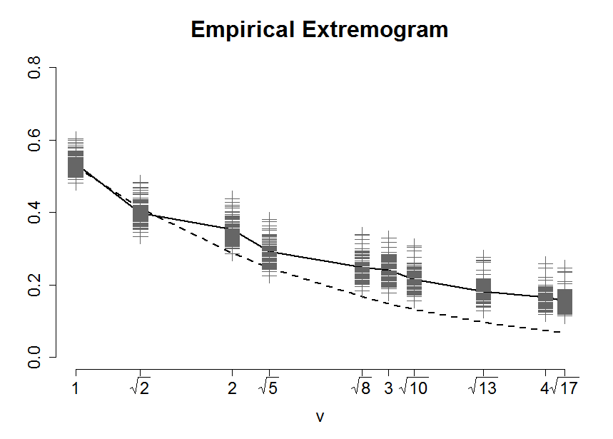
Refer to caption
(a)
Refer to caption
(b)
Figure 1: Empirical spatial extremogram (left) and its bias corrected version (right) for 100 simulated max-stable random fields in (4.1) with δ(v,0)=20.4v1.5𝛿𝑣020.4superscript𝑣1.5\delta(v,0)=2\cdot 0.4v^{1.5}. The dashed line represents the theoretical spatial extremogram and the solid line is the mean over all 100 replicates.

4.2 Asymptotic properties of spatial parameter estimates of the Brown-Resnick process

In this section we prove asymptotic normality of the WLSE (θ^1,α^1)subscript^𝜃1subscript^𝛼1(\widehat{\theta}_{1},\widehat{\alpha}_{1}). We proceed as in the more general setting in Section 3.2. Recall that in the more specific situation here we have C1=log(θ1)subscript𝐶1subscript𝜃1C_{1}=\log(\theta_{1}) and choose the transformation T1(χ(v,0))=2log(Φ1(112χ(v,0)))subscript𝑇1𝜒𝑣02superscriptΦ1112𝜒𝑣0T_{1}(\chi(v,0))=2\log\big{(}\Phi^{-1}\big{(}1-\frac{1}{2}\chi(v,0)\big{)}\big{)}, where the log transformed version of the spatial lag satisfies xv=log(v)0subscript𝑥𝑣𝑣0x_{v}=\log(v)\geq 0 for v𝒱𝑣𝒱v\in{\mathcal{V}}. We set χ~(v,0)=1Tk=1Tχ~(tk)(v,0)~𝜒𝑣01𝑇superscriptsubscript𝑘1𝑇superscript~𝜒subscript𝑡𝑘𝑣0\widetilde{\chi}(v,0)=\frac{1}{T}\sum_{k=1}^{T}\widetilde{\chi}^{(t_{k})}(v,0) as in (2.7), possibly after a bias correction, which depends on the two cases described in Remark 4.1. The analogue of the weighted least squares optimization problem (2.9) then reads as

(θ^1α^1)=argminα1(0,2]θ1,α1>0matrixsubscript^𝜃1subscript^𝛼1subscriptargminsuperscriptsubscript𝛼102subscript𝜃1subscript𝛼10\displaystyle\begin{pmatrix}\widehat{\theta}_{1}\\ \widehat{\alpha}_{1}\end{pmatrix}=\operatorname*{arg\,min}_{\stackrel{{\scriptstyle\theta_{1},\alpha_{1}>0}}{{\alpha_{1}\in(0,2]}}} v𝒱wv(T1(χ~(v,0))(log(θ1)+α1xv))2.subscript𝑣𝒱subscript𝑤𝑣superscriptsubscript𝑇1~𝜒𝑣0subscript𝜃1subscript𝛼1subscript𝑥𝑣2\displaystyle\sum_{v\in{\mathcal{V}}}w_{v}\big{(}T_{1}(\widetilde{\chi}(v,0))-\big{(}\log(\theta_{1})+\alpha_{1}x_{v}\big{)}\big{)}^{2}. (4.14)

Note in particular that α1subscript𝛼1\alpha_{1} has bounded support; this has to be treated as a special case in what follows. To show asymptotic normality of the WLSE in (4.14), we define as before design and weight matrices X𝑋X and W𝑊W as

X=[𝟏,(xv)]v𝒱p×2 and W=diag{wv:v𝒱}p×p,X=[\boldsymbol{1},(x_{v}){}^{{}^{\intercal}}_{v\in{\mathcal{V}}}]\in\mathbb{R}^{p\times 2}\quad\text{ and }\quad W=\operatorname*{diag}\{w_{v}:v\in{\mathcal{V}}\}\in\mathbb{R}^{p\times p},

respectively, where 𝟏=(1,,1)p\boldsymbol{1}=(1,\ldots,1){}^{{}^{\intercal}}\in\mathbb{R}^{p}. Let 𝝍1=(log(θ1),α1)\boldsymbol{\psi}_{1}=(\log(\theta_{1}),\alpha_{1}){}^{{}^{\intercal}} be the parameter vector with parameter space Θ𝒮=×(0,2]subscriptΘ𝒮02\Theta_{{\mathcal{S}}}=\mathbb{R}\times(0,2]. Then the WLSE; i.e., the solution to (4.14) is given by

𝝍^1=(log(θ^1)α^1)=(XWX)1XW(T1(χ~(v,0))).v𝒱\displaystyle\widehat{\boldsymbol{\psi}}_{1}=\begin{pmatrix}\log(\widehat{\theta}_{1})\\ \widehat{\alpha}_{1}\end{pmatrix}=(X{}^{{}^{\intercal}}WX)^{-1}X{}^{{}^{\intercal}}W(T_{1}(\widetilde{\chi}(v,0))){}^{{}^{\intercal}}_{v\in{\mathcal{V}}}. (4.15)

Without any constraints 𝝍^1subscript^𝝍1\widehat{\boldsymbol{\psi}}_{1} may produce estimates of α1subscript𝛼1\alpha_{1} outside its parameter space (0,2]02(0,2]. In such cases we set the parameter estimate equal to 2, and we denote the resulting estimate by 𝝍^1c=(log(θ^1c),α^1c)\boldsymbol{\widehat{\psi}}_{1}^{c}=(\log(\widehat{\theta}_{1}^{c}),\widehat{\alpha}_{1}^{c}){}^{{}^{\intercal}}.

Theorem 4.6.

Let 𝛙^1c=(log(θ^1c),α^1c)\boldsymbol{\widehat{\psi}}_{1}^{c}=(\log(\widehat{\theta}_{1}^{c}),\widehat{\alpha}_{1}^{c}){}^{{}^{\intercal}} denote the WLSE resulting from the constrained minimization problem (4.14) and 𝛙1=(log(θ1),α1)Θ𝒮\boldsymbol{\psi}^{*}_{1}=(\log(\theta_{1}^{*}),\alpha_{1}^{*}){}^{{}^{\intercal}}\in\Theta_{{\mathcal{S}}} the true parameter vector. Set mn=nβ1subscript𝑚𝑛superscript𝑛subscript𝛽1m_{n}=n^{\beta_{1}} for β1(1/5,1/2)subscript𝛽11512\beta_{1}\in(1/5,1/2). Then as n𝑛n\to\infty,

nmn(𝝍^1c𝝍1)d{𝒁1if α1<2,𝒁2if α1=2,superscript𝑑𝑛subscript𝑚𝑛superscriptsubscriptbold-^𝝍1𝑐superscriptsubscript𝝍1casessubscript𝒁1if superscriptsubscript𝛼12subscript𝒁2if superscriptsubscript𝛼12\frac{n}{m_{n}}\Big{(}\boldsymbol{\widehat{\psi}}_{1}^{c}-\boldsymbol{\psi}_{1}^{*}\Big{)}\stackrel{{\scriptstyle d}}{{\to}}\begin{cases}\boldsymbol{Z}_{1}\quad&\mbox{if }\alpha_{1}^{*}<2,\\ \boldsymbol{Z}_{2}\quad&\mbox{if }\alpha_{1}^{*}=2,\end{cases} (4.16)

where 𝐙1𝒩(𝟎,Π3(iso))similar-tosubscript𝐙1𝒩0subscriptsuperscriptΠiso3\boldsymbol{Z}_{1}\sim\mathcal{N}(\boldsymbol{0},\Pi^{(\textnormal{iso})}_{3}), and the distribution of 𝐙2subscript𝐙2\boldsymbol{Z}_{2} is given by

(𝒁2B)=B{(b1,b2)2:b2<0}φ𝟎,Π3(iso)(z1,z2)𝑑z1𝑑z2subscript𝒁2𝐵subscript𝐵conditional-setsubscript𝑏1subscript𝑏2superscript2subscript𝑏20subscript𝜑0subscriptsuperscriptΠiso3subscript𝑧1subscript𝑧2differential-dsubscript𝑧1differential-dsubscript𝑧2\displaystyle\mathbb{P}\left(\boldsymbol{Z}_{2}\in B\right)=\int_{B\cap\left\{(b_{1},b_{2})\in\mathbb{R}^{2}:b_{2}<0\right\}}\varphi_{\boldsymbol{0},\Pi^{(\textnormal{iso})}_{3}}(z_{1},z_{2})dz_{1}dz_{2} (4.17)
+0{b1:(b1,0)B}φ𝟎,Π3(iso)(z11v𝒱wvv𝒱(wvxv)z2,z2)𝑑z1𝑑z2superscriptsubscript0subscriptconditional-setsubscript𝑏1subscript𝑏10𝐵subscript𝜑0subscriptsuperscriptΠiso3subscript𝑧11subscript𝑣𝒱subscript𝑤𝑣subscript𝑣𝒱subscript𝑤𝑣subscript𝑥𝑣subscript𝑧2subscript𝑧2differential-dsubscript𝑧1differential-dsubscript𝑧2\displaystyle\qquad\qquad+\int_{0}^{\infty}\int_{\{b_{1}\in\mathbb{R}:(b_{1},0)\in B\}}\varphi_{\boldsymbol{0},\Pi^{(\textnormal{iso})}_{3}}\Big{(}z_{1}-\frac{1}{\sum_{v\in{\mathcal{V}}}w_{v}}\sum_{v\in{\mathcal{V}}}(w_{v}x_{v})\ z_{2},\,z_{2}\Big{)}dz_{1}dz_{2}

for every Borel set B𝐵B in 2superscript2\mathbb{R}^{2}, and φ𝟎,Σsubscript𝜑0Σ\varphi_{\boldsymbol{0},\Sigma} denotes the bivariate normal density with mean vector 𝟎0\boldsymbol{0} and covariance matrix ΣΣ\Sigma. In particular, the joint distribution function of 𝐙2subscript𝐙2\boldsymbol{Z}_{2} is given for (p1,p2)2(p_{1},p_{2}){}^{{}^{\intercal}}\in\mathbb{R}^{2} by

(𝒁2(p1,p2))=min{0,p2}p1φ𝟎,Π3(iso)(z1,z2)dz1dz2\displaystyle\mathbb{P}\left(\boldsymbol{Z}_{2}\leq(p_{1},p_{2}){}^{{}^{\intercal}}\right)=\int\limits_{-\infty}^{\min\{0,p_{2}\}}\int\limits_{-\infty}^{p_{1}}\varphi_{\boldsymbol{0},\Pi^{(\textnormal{iso})}_{3}}(z_{1},z_{2})dz_{1}dz_{2} (4.18)
+𝟙{p20}0p1φ𝟎,Π3(iso)(z11v𝒱wvv𝒱(wvxv)z2,z2)𝑑z1𝑑z2.subscript1subscript𝑝20superscriptsubscript0superscriptsubscriptsubscript𝑝1subscript𝜑0subscriptsuperscriptΠiso3subscript𝑧11subscript𝑣𝒱subscript𝑤𝑣subscript𝑣𝒱subscript𝑤𝑣subscript𝑥𝑣subscript𝑧2subscript𝑧2differential-dsubscript𝑧1differential-dsubscript𝑧2\displaystyle\qquad\qquad+\mathbbmss{1}_{\{p_{2}\geq 0\}}\int\limits_{0}^{\infty}\int\limits_{-\infty}^{p_{1}}\varphi_{\boldsymbol{0},\Pi^{(\textnormal{iso})}_{3}}\Big{(}z_{1}-\frac{1}{\sum_{v\in{\mathcal{V}}}w_{v}}\sum_{v\in{\mathcal{V}}}(w_{v}x_{v})\ z_{2},\,z_{2}\Big{)}dz_{1}dz_{2}.

The covariance matrix of 𝐙1subscript𝐙1\boldsymbol{Z}_{1} has representation

Π3(iso)=Qx(w)GΠ2(iso)GQx(w),\Pi^{(\textnormal{iso})}_{3}=Q_{x}^{(w)}G\Pi^{(\textnormal{iso})}_{2}G{Q_{x}^{(w)}}{}^{{}^{\intercal}}, (4.19)

where Π2(iso)subscriptsuperscriptΠiso2\Pi^{(\textnormal{iso})}_{2} is the covariance matrix given in (3.1),

Qx(w)superscriptsubscript𝑄𝑥𝑤\displaystyle Q_{x}^{(w)} =(XWX)1XW andG=diag{2πθ1vα1exp{12θ1vα1}:v𝒱}.formulae-sequenceabsentsuperscript𝑋superscript𝑊𝑋1𝑋superscript𝑊 and𝐺diag:2𝜋superscriptsubscript𝜃1superscript𝑣superscriptsubscript𝛼112superscriptsubscript𝜃1superscript𝑣superscriptsubscript𝛼1𝑣𝒱\displaystyle=(X{}^{{}^{\intercal}}WX)^{-1}X{}^{{}^{\intercal}}W\quad\text{ and}\quad G=\operatorname*{diag}\bigg{\{}\sqrt{\frac{2\pi}{\theta_{1}^{*}v^{\alpha_{1}^{*}}}}\exp\Big{\{}\frac{1}{2}\theta_{1}^{*}v^{\alpha_{1}^{*}}\Big{\}}:\ v\in{\mathcal{V}}\hskip 2.84544pt\bigg{\}}.
Proof.

For the first part of the proof, we neglect the constraints on α1subscript𝛼1\alpha_{1}. Then we can directly use Theorem 3.4, observing that the derivative of T1subscript𝑇1T_{1} is given by

T1(x)=(Φ1(1x2)φ(Φ1(1x2)))1,0<x<1,formulae-sequencesuperscriptsubscript𝑇1𝑥superscriptsuperscriptΦ11𝑥2𝜑superscriptΦ11𝑥210𝑥1T_{1}^{\prime}(x)=-\Big{(}\Phi^{-1}(1-\frac{x}{2})\,\varphi(\Phi^{-1}(1-\frac{x}{2}))\Big{)}^{-1},\quad 0<x<1,

where φ𝜑\varphi is the univariate standard normal density. Thus,

T1(χ(v,0))=(θ1vα1φ(θ1vα1))1=2πθ1vα1exp{12θ1vα1}.superscriptsubscript𝑇1𝜒𝑣0superscriptsuperscriptsubscript𝜃1superscript𝑣superscriptsubscript𝛼1𝜑superscriptsubscript𝜃1superscript𝑣superscriptsubscript𝛼112𝜋superscriptsubscript𝜃1superscript𝑣superscriptsubscript𝛼112superscriptsubscript𝜃1superscript𝑣superscriptsubscript𝛼1T_{1}^{\prime}(\chi(v,0))=-\Big{(}\sqrt{\theta_{1}^{*}v^{\alpha_{1}^{*}}}\,\varphi\big{(}\sqrt{\theta_{1}^{*}v^{\alpha_{1}^{*}}}\big{)}\Big{)}^{-1}=-\sqrt{\frac{2\pi}{\theta_{1}^{*}v^{\alpha_{1}^{*}}}}\exp\Big{\{}\frac{1}{2}\theta_{1}^{*}v^{\alpha_{1}^{*}}\Big{\}}.

Hence, as n𝑛n\to\infty,

nmn(𝝍^1𝝍1)=nmnQx(w)(T1(χ~(v,0))T1(χ(v,0)))v𝒱d𝒩(𝟎,Qx(w)GΠ2(iso)GQx(w)).\frac{n}{m_{n}}\left(\boldsymbol{\widehat{\psi}}_{1}-\boldsymbol{\psi}_{1}^{*}\right)=\frac{n}{m_{n}}Q_{x}^{(w)}\big{(}T_{1}(\widetilde{\chi}(v,0))-T_{1}(\chi(v,0))\big{)}_{v\in{\mathcal{V}}}\stackrel{{\scriptstyle d}}{{\to}}\mathcal{N}\left(\boldsymbol{0},Q_{x}^{(w)}G\Pi^{(\textnormal{iso})}_{2}G{Q_{x}^{(w)}}{}^{{}^{\intercal}}\right).

Note that we can define the diagonal matrix G𝐺G unsigned, since signs cancel out. We now turn to the constraints on α1subscript𝛼1\alpha_{1}. Since the objective function is quadratic, if the unconstrained estimate exceeds two, the constraint α1(0,2]subscript𝛼102\alpha_{1}\in(0,2] results in an estimate α^1c=2superscriptsubscript^𝛼1𝑐2\widehat{\alpha}_{1}^{c}=2. We consider separately the cases α1<2superscriptsubscript𝛼12\alpha_{1}^{*}<2 and α1=2superscriptsubscript𝛼12\alpha_{1}^{*}=2; i.e., the true parameter lies either in the interior or on the boundary of the parameter space. The constrained estimator 𝝍^1csuperscriptsubscriptbold-^𝝍1𝑐\boldsymbol{\widehat{\psi}}_{1}^{c} can be written as

𝝍^1c=𝝍^1𝟙{α^12}+(θ^1,2)𝟙{α^1>2}.\boldsymbol{\widehat{\psi}}_{1}^{c}=\boldsymbol{\widehat{\psi}}_{1}\mathds{1}_{\left\{\widehat{\alpha}_{1}\leq 2\right\}}+(\widehat{\theta}_{1},2){}^{{}^{\intercal}}\mathds{1}_{\left\{\widehat{\alpha}_{1}>2\right\}}.

We calculate the asymptotic probabilities for the events {α^12}subscript^𝛼12\{\widehat{\alpha}_{1}\leq 2\} and {α^1>2}subscript^𝛼12\{\widehat{\alpha}_{1}>2\},

(α^12)subscript^𝛼12\displaystyle\mathbb{P}(\widehat{\alpha}_{1}\leq 2) =(nmn(α^1α1)nmn(2α1)).absent𝑛subscript𝑚𝑛subscript^𝛼1superscriptsubscript𝛼1𝑛subscript𝑚𝑛2superscriptsubscript𝛼1\displaystyle=\mathbb{P}\Big{(}\frac{n}{m_{n}}(\widehat{\alpha}_{1}-\alpha_{1}^{*})\leq\frac{n}{m_{n}}(2-\alpha_{1}^{*})\Big{)}.

Since for α1<2superscriptsubscript𝛼12\alpha_{1}^{*}<2 as n𝑛n\to\infty

nmn(α^1α1)d𝒩(0,(0,1)Π3(iso)(0,1))andnmn(2α1),\frac{n}{m_{n}}\big{(}\widehat{\alpha}_{1}-\alpha_{1}^{*}\big{)}\stackrel{{\scriptstyle d}}{{\to}}\mathcal{N}\left(0,{(0,1)}\Pi^{(\textnormal{iso})}_{3}{(0,1){}^{{}^{\intercal}}}\right)\quad\mbox{and}\quad\frac{n}{m_{n}}(2-\alpha_{1}^{*})\to\infty,

it follows that

(α^12)1and(α^1>2)0,n.formulae-sequencesubscript^𝛼121andformulae-sequencesubscript^𝛼120𝑛\mathbb{P}(\widehat{\alpha}_{1}\leq 2)\to 1\quad\text{and}\quad\mathbb{P}(\widehat{\alpha}_{1}>2)\to 0,\quad n\to\infty. (4.20)

Therefore, for α1<2superscriptsubscript𝛼12\alpha_{1}^{*}<2,

nmn(𝝍^1c𝝍1)d𝒩(𝟎,Π3(iso)),n.formulae-sequencesuperscript𝑑𝑛subscript𝑚𝑛subscriptsuperscriptbold-^𝝍𝑐1superscriptsubscript𝝍1𝒩0subscriptsuperscriptΠ(iso)3𝑛\frac{n}{m_{n}}\big{(}\boldsymbol{\widehat{\psi}}^{c}_{1}-\boldsymbol{\psi}_{1}^{*}\big{)}\stackrel{{\scriptstyle d}}{{\to}}\mathcal{N}(\boldsymbol{0},\Pi^{\textnormal{(iso)}}_{3}),\quad n\to\infty.

We now consider the case α1=2superscriptsubscript𝛼12\alpha_{1}^{*}=2 and α^1>2subscript^𝛼12\widehat{\alpha}_{1}>2 (the unconstrained estimate exceeds 2). In this case (4.14) leads to the constrained optimization problem

min𝝍1{[W1/2((T1(χ~(v,0)))v𝒱X𝝍1)][W1/2((T1(χ~(v,0)))v𝒱X𝝍1]},\displaystyle\min_{\boldsymbol{\psi}_{1}}\{[W^{1/2}((T_{1}(\widetilde{\chi}(v,0))){}^{{}^{\intercal}}_{v\in{\mathcal{V}}}-X\boldsymbol{\psi}_{1})]{}^{{}^{\intercal}}[W^{1/2}((T_{1}(\widetilde{\chi}(v,0))){}^{{}^{\intercal}}_{v\in{\mathcal{V}}}-X\boldsymbol{\psi}_{1}]\},
s.t.(0,1)𝝍1=2.s.t.01subscript𝝍12\displaystyle\quad\text{s.t.}\quad(0,1)\boldsymbol{\psi}_{1}=2.

To obtain asymptotic results for 𝝍^1c𝝍1subscriptsuperscriptbold-^𝝍𝑐1superscriptsubscript𝝍1\boldsymbol{\widehat{\psi}}^{c}_{1}-\boldsymbol{\psi}_{1}^{*}, the vector 𝝍^1𝝍1subscriptbold-^𝝍1superscriptsubscript𝝍1\boldsymbol{\widehat{\psi}}_{1}-\boldsymbol{\psi}_{1}^{*} is projected onto the line Λ={𝝍2,(0,1)𝝍=0}Λformulae-sequence𝝍superscript201𝝍0\Lambda=\{\boldsymbol{\psi}\in\mathbb{R}^{2},(0,1)\boldsymbol{\psi}=0\}, i.e., denoting by I2subscript𝐼2I_{2} the 2×2222\times 2-identity matrix, the projection matrix with respect to the induced norm 𝝍(𝝍XWX𝝍)1/2maps-to𝝍superscript𝝍superscript𝑋superscript𝑊𝑋𝝍12\boldsymbol{\psi}\mapsto(\boldsymbol{\psi}{}^{{}^{\intercal}}X{}^{{}^{\intercal}}WX\boldsymbol{\psi})^{1/2} is given by (cf. Andrews [1], page 1365)

PΛ=I2(XWX)1(0,1)((0,1)(XWX)1(0,1))1(0,1).P_{\Lambda}=I_{2}-(X{}^{{}^{\intercal}}WX)^{-1}(0,1){}^{{}^{\intercal}}((0,1)(X{}^{{}^{\intercal}}WX)^{-1}(0,1){}^{{}^{\intercal}})^{-1}(0,1).

For simplicity we use the abbreviation pwx=v𝒱wvxv/v𝒱wvsubscript𝑝𝑤𝑥subscript𝑣𝒱subscript𝑤𝑣subscript𝑥𝑣subscript𝑣𝒱subscript𝑤𝑣p_{wx}=\sum_{v\in{\mathcal{V}}}w_{v}x_{v}/\sum_{v\in{\mathcal{V}}}w_{v}. We calculate

(𝝍^1c𝝍1)𝟙{α^1>2}=PΛ(𝝍^1𝝍1)𝟙{α^1>2}subscriptsuperscriptbold-^𝝍𝑐1subscriptsuperscript𝝍1subscript1subscript^𝛼12subscript𝑃Λsubscriptbold-^𝝍1superscriptsubscript𝝍1subscript1subscript^𝛼12\displaystyle(\boldsymbol{\widehat{\psi}}^{c}_{1}-\boldsymbol{\psi}^{*}_{1})\mathds{1}_{\{\widehat{\alpha}_{1}>2\}}=P_{\Lambda}(\boldsymbol{\widehat{\psi}}_{1}-\boldsymbol{\psi}_{1}^{*})\mathds{1}_{\{\widehat{\alpha}_{1}>2\}}
=(𝝍^1𝝍1)𝟙{α^1>2}(XWX)1(0,1)((0,1)(XWX)1(0,1))1(α^12)𝟙{α^1>2}\displaystyle=(\boldsymbol{\widehat{\psi}}_{1}-\boldsymbol{\psi}_{1}^{*})\mathds{1}_{\{\widehat{\alpha}_{1}>2\}}-(X{}^{{}^{\intercal}}WX)^{-1}(0,1){}^{{}^{\intercal}}\left((0,1)(X{}^{{}^{\intercal}}WX)^{-1}(0,1){}^{{}^{\intercal}}\right)^{-1}(\widehat{\alpha}_{1}-2)\mathds{1}_{\{\widehat{\alpha}_{1}>2\}}
=(𝝍^1𝝍1)𝟙{α^1>2}+(pwx1)(α^12)𝟙{α^1>2}.absentsubscriptbold-^𝝍1superscriptsubscript𝝍1subscript1subscript^𝛼12matrixsubscript𝑝𝑤𝑥1subscript^𝛼12subscript1subscript^𝛼12\displaystyle=(\boldsymbol{\widehat{\psi}}_{1}-\boldsymbol{\psi}_{1}^{*})\mathds{1}_{\{\widehat{\alpha}_{1}>2\}}+\begin{pmatrix}p_{wx}\\ -1\end{pmatrix}(\widehat{\alpha}_{1}-2)\mathds{1}_{\{\widehat{\alpha}_{1}>2\}}.

For the joint constrained estimator 𝝍1csuperscriptsubscript𝝍1𝑐\boldsymbol{\psi}_{1}^{c} we obtain

𝝍^1c𝝍1subscriptsuperscriptbold-^𝝍𝑐1superscriptsubscript𝝍1\displaystyle\boldsymbol{\widehat{\psi}}^{c}_{1}-\boldsymbol{\psi}_{1}^{*} =(𝝍^1c𝝍1)𝟙{α^12}+(𝝍^1c𝝍1)𝟙{α^1>2}absentsubscriptsuperscriptbold-^𝝍𝑐1superscriptsubscript𝝍1subscript1subscript^𝛼12subscriptsuperscriptbold-^𝝍𝑐1superscriptsubscript𝝍1subscript1subscript^𝛼12\displaystyle=(\boldsymbol{\widehat{\psi}}^{c}_{1}-\boldsymbol{\psi}_{1}^{*})\mathds{1}_{\{\widehat{\alpha}_{1}\leq 2\}}+(\boldsymbol{\widehat{\psi}}^{c}_{1}-\boldsymbol{\psi}_{1}^{*})\mathds{1}_{\{\widehat{\alpha}_{1}>2\}}
=(𝝍^1𝝍1)𝟙{α^12}+(𝝍^1𝝍1)𝟙{α^1>2}+(pwx1)(α^12)𝟙{α^1>2}absentsubscriptbold-^𝝍1superscriptsubscript𝝍1subscript1subscript^𝛼12subscriptbold-^𝝍1superscriptsubscript𝝍1subscript1subscript^𝛼12matrixsubscript𝑝𝑤𝑥1subscript^𝛼12subscript1subscript^𝛼12\displaystyle=(\boldsymbol{\widehat{\psi}}_{1}-\boldsymbol{\psi}_{1}^{*})\mathds{1}_{\{\widehat{\alpha}_{1}\leq 2\}}+(\boldsymbol{\widehat{\psi}}_{1}-\boldsymbol{\psi}_{1}^{*})\mathds{1}_{\{\widehat{\alpha}_{1}>2\}}+\begin{pmatrix}p_{wx}\\ -1\end{pmatrix}(\widehat{\alpha}_{1}-2)\mathds{1}_{\{\widehat{\alpha}_{1}>2\}}
=(𝝍^1𝝍1)+(pwx1)(α^12)𝟙{α^1>2}.absentsubscriptbold-^𝝍1superscriptsubscript𝝍1matrixsubscript𝑝𝑤𝑥1subscript^𝛼12subscript1subscript^𝛼12\displaystyle=(\boldsymbol{\widehat{\psi}}_{1}-\boldsymbol{\psi}_{1}^{*})+\begin{pmatrix}p_{wx}\\ -1\end{pmatrix}(\widehat{\alpha}_{1}-2)\mathds{1}_{\{\widehat{\alpha}_{1}>2\}}.

This implies

nmn(𝝍^1c𝝍1)𝑛subscript𝑚𝑛subscriptsuperscriptbold-^𝝍𝑐1superscriptsubscript𝝍1\displaystyle\frac{n}{m_{n}}(\boldsymbol{\widehat{\psi}}^{c}_{1}-\boldsymbol{\psi}_{1}^{*}) =nmn((log(θ^1)log(θ1))+pwx(α^12)𝟙{α^1>2}(α^12)(α^12)𝟙{α^1>2}).absent𝑛subscript𝑚𝑛matrixsubscript^𝜃1superscriptsubscript𝜃1subscript𝑝𝑤𝑥subscript^𝛼12subscript1subscript^𝛼12subscript^𝛼12subscript^𝛼12subscript1subscript^𝛼12\displaystyle=\frac{n}{m_{n}}\begin{pmatrix}(\log(\widehat{\theta}_{1})-\log(\theta_{1}^{*}))+p_{wx}(\widehat{\alpha}_{1}-2)\mathds{1}_{\{\widehat{\alpha}_{1}>2\}}\\ (\widehat{\alpha}_{1}-2)-(\widehat{\alpha}_{1}-2)\mathds{1}_{\{\widehat{\alpha}_{1}>2\}}\end{pmatrix}.

Let f(x1,x2)=(x1+pwxx2𝟙{x2>0},x2x2𝟙{x2>0})f(x_{1},x_{2})=(x_{1}+p_{wx}x_{2}\mathds{1}_{\{x_{2}>0\}},x_{2}-x_{2}\mathds{1}_{\{x_{2}>0\}}){}^{{}^{\intercal}} and observe that f(c(x1,x2))=cf(x1,x2)𝑓𝑐subscript𝑥1subscript𝑥2𝑐𝑓subscript𝑥1subscript𝑥2f(c(x_{1},x_{2}))=cf(x_{1},x_{2}) for c0.𝑐0c\geq 0. For the asymptotic distribution we calculate, denoting by f1superscript𝑓1f^{-1} the inverse image of f𝑓f,

(nmn(𝝍^1c𝝍1)B)𝑛subscript𝑚𝑛subscriptsuperscriptbold-^𝝍𝑐1superscriptsubscript𝝍1𝐵\displaystyle\mathbb{P}\Big{(}\frac{n}{m_{n}}(\boldsymbol{\widehat{\psi}}^{c}_{1}-\boldsymbol{\psi}_{1}^{*})\in B\Big{)}
=(nmnf(𝝍^1𝝍1)B)=(f(nmn(𝝍^1𝝍1))B)absent𝑛subscript𝑚𝑛𝑓subscriptbold-^𝝍1superscriptsubscript𝝍1𝐵𝑓𝑛subscript𝑚𝑛subscriptbold-^𝝍1superscriptsubscript𝝍1𝐵\displaystyle=\mathbb{P}\Big{(}\frac{n}{m_{n}}f(\boldsymbol{\widehat{\psi}}_{1}-\boldsymbol{\psi}_{1}^{*})\in B\Big{)}=\mathbb{P}\Big{(}f\big{(}\frac{n}{m_{n}}(\boldsymbol{\widehat{\psi}}_{1}-\boldsymbol{\psi}_{1}^{*})\big{)}\in B\Big{)}
=(nmn(𝝍^1𝝍1)f1(B{(b1,b2)2:b2<0})f1(B{(b1,0):b1}))absent𝑛subscript𝑚𝑛subscriptbold-^𝝍1superscriptsubscript𝝍1superscript𝑓1𝐵conditional-setsubscript𝑏1subscript𝑏2superscript2subscript𝑏20superscript𝑓1𝐵conditional-setsubscript𝑏10subscript𝑏1\displaystyle=\mathbb{P}\Big{(}\frac{n}{m_{n}}(\boldsymbol{\widehat{\psi}}_{1}-\boldsymbol{\psi}_{1}^{*})\in f^{-1}(B\cap\{(b_{1},b_{2})\in\mathbb{R}^{2}:b_{2}<0\})\cup f^{-1}(B\cap\{(b_{1},0):b_{1}\in\mathbb{R}\})\Big{)}
=(nmn(𝝍^1𝝍1)[B{(b1,b2)2:b2<0}]\displaystyle=\mathbb{P}\Big{(}\frac{n}{m_{n}}(\boldsymbol{\widehat{\psi}}_{1}-\boldsymbol{\psi}_{1}^{*})\in[B\cap\{(b_{1},b_{2})\in\mathbb{R}^{2}:b_{2}<0\}]
[{(b1pwxb2,b2),b20,(b1,0)B}])\displaystyle\quad\quad\cup[\{(b_{1}-p_{wx}b_{2},b_{2}),b_{2}\geq 0,(b_{1},0)\in B\}]\Big{)}
B{(b1,b2)2,b2<0}φ𝟎,Π3(iso)(z1,z2)𝑑z1𝑑z2absentsubscript𝐵formulae-sequencesubscript𝑏1subscript𝑏2superscript2subscript𝑏20subscript𝜑0subscriptsuperscriptΠiso3subscript𝑧1subscript𝑧2differential-dsubscript𝑧1differential-dsubscript𝑧2\displaystyle\to\int_{B\cap\left\{(b_{1},b_{2})\in\mathbb{R}^{2},b_{2}<0\right\}}\varphi_{\boldsymbol{0},\Pi^{(\textnormal{iso})}_{3}}(z_{1},z_{2})dz_{1}dz_{2}
+0{b1,(b1,0)B}φ𝟎,Π3(iso)(z1pwxz2,z2)𝑑z1𝑑z2,n.superscriptsubscript0subscriptformulae-sequencesubscript𝑏1subscript𝑏10𝐵subscript𝜑0subscriptsuperscriptΠiso3subscript𝑧1subscript𝑝𝑤𝑥subscript𝑧2subscript𝑧2differential-dsubscript𝑧1differential-dsubscript𝑧2𝑛\displaystyle\qquad\qquad+\int_{0}^{\infty}\int_{\{b_{1}\in\mathbb{R},(b_{1},0)\in B\}}\varphi_{\boldsymbol{0},\Pi^{(\textnormal{iso})}_{3}}(z_{1}-p_{wx}z_{2},z_{2})dz_{1}dz_{2},\quad n\to\infty.

Plugging in B=(,p1]×(,p2]𝐵subscript𝑝1subscript𝑝2B=(-\infty,p_{1}]\times(-\infty,p_{2}] and using the Fubini-Tonelli theorem yields (4.18). ∎

Remark 4.3.

The asymptotic properties for the constrained estimate are derived as a special case of Corollary 1 in Andrews [1], who shows asymptotic properties of parameter estimates in a very general setting, when the true parameter is on the boundary of the parameter space. The asymptotic distribution of the estimates for α1=2superscriptsubscript𝛼12\alpha_{1}^{*}=2 results from the fact that approximately half of the estimates lie above the true value and are therefore equal to two.   \Box

5 Analysis of radar rainfall measurements

Finally, we apply the Brown-Resnick space-time process in (4.1) and the WLSE to radar rainfall data provided by the Southwest Florida Water Management District (SWFWMD)111http://www.swfwmd.state.fl.us/. Our objective is to quantify their extremal behaviour by using spatial and temporal block maxima and fitting a Brown-Resnick space-time process to the block maxima.

The data base consists of radar values in inches measured on a 120×120120120120\times 120km region containing 3600 grid locations. We calculate the spatial and temporal maxima over subregions of size 10×10101010\times 10km and over 24 subsequent measurements of the corresponding hourly accumulated time series in the wet season (June to September) from the years 1999-2004. In this way we obtain 12×12121212\times 12 locations on 732732732 days of space-time block maxima of rainfall observations. Taking block maxima yields a process consistent with the assumption of a max-stable process, or at least to lie in the domain of attraction of a max-stable process. Taking daily data, we can furthermore ignore diurnal patterns.

We denote the set of locations by 𝒮={(i1,i2),i1,i2{1,,12}}𝒮subscript𝑖1subscript𝑖2subscript𝑖1subscript𝑖2112{\mathcal{S}}=\{(i_{1},i_{2}),i_{1},i_{2}\in\{1,\ldots,12\}\} and the space-time observations by {η(𝒔,t),𝒔𝒮,t{t1,,t732}}formulae-sequence𝜂𝒔𝑡𝒔𝒮𝑡subscript𝑡1subscript𝑡732\{\eta(\boldsymbol{s},t),\boldsymbol{s}\in{\mathcal{S}},t\in\{t_{1},\ldots,t_{732}\}\}. This setup is also considered in Buhl and Klüppelberg [4], Section 5, and Steinkohl [27], Chapter 7. To make the results obtained there comparable to ours, we use the the same preprocessing steps; for a precise description cf. [4], Section 5.1.

The data do not fail the max-stability check described in Section 5.2 of [4], such that we assume that {η(𝒔,t),𝒔𝒮,t{t1,,t732}}formulae-sequence𝜂𝒔𝑡𝒔𝒮𝑡subscript𝑡1subscript𝑡732\{\eta(\boldsymbol{s},t),\boldsymbol{s}\in{\mathcal{S}},t\in\{t_{1},\ldots,t_{732}\}\} are realizations of a max-stable space-time process with standard unit Fréchet margins. Nevertheless, the assumption that the data are in fact an exact realization from a max-stable process is only approximate. Hence there is no guarantee that composite likelihood estimation applied to these transformed data outperforms the semiparametric estimation introduced in Section 2; cf. the results obtained in Section 10 of the supplement [7] when data have observational noise. Here we use this data example to illustrate our new semiparametric methodology.

We fit the Brown-Resnick process (4.1) by estimating (4.2) as follows:

  1. (1)

    We estimate the parameters θ1subscript𝜃1\theta_{1}, α1subscript𝛼1\alpha_{1}, θ2subscript𝜃2\theta_{2} and α2subscript𝛼2\alpha_{2} by WLSE as described in Section 2 based on the sets 𝒱={1,2,2,5,8,3,10,13,4,17}𝒱1225831013417{\mathcal{V}}=\{1,\sqrt{2},2,\sqrt{5},\sqrt{8},3,\sqrt{10},\sqrt{13},4,\sqrt{17}\} and 𝒰={1,,10}𝒰110{\mathcal{U}}=\{1,\ldots,10\}. Permutation tests as described below and visualized in Figure 4 indicate that these lags are sufficient to cover the relevant extremal dependence structure. We choose as weights for the different spatial and temporal lags v𝒱𝑣𝒱v\in{\mathcal{V}} and u𝒰𝑢𝒰u\in{\mathcal{U}} the corresponding estimated averaged extremogram values; i.e., wv=T1k=1Tχ~(tk)(v,0)subscript𝑤𝑣superscript𝑇1superscriptsubscript𝑘1𝑇superscript~𝜒subscript𝑡𝑘𝑣0w_{v}=T^{-1}\sum_{k=1}^{T}\widetilde{\chi}^{(t_{k})}(v,0) and wu=n2i=1n2χ~(𝒔i)(0,u)subscript𝑤𝑢superscript𝑛2superscriptsubscript𝑖1superscript𝑛2superscript~𝜒subscript𝒔𝑖0𝑢w_{u}=n^{-2}\sum_{i=1}^{n^{2}}\widetilde{\chi}^{(\boldsymbol{s}_{i})}(0,u), respectively. Since the so defined weights are random, what follows is conditional on the realizations of these weights.

    As the number of spatial points in the analysis is rather small, we cannot choose a very high empirical quantile q𝑞q, since this would in turn result in a too small number of exceedances to get a reliable estimate of the extremogram. Hence, we choose q𝑞q as the empirical 60%limit-frompercent6060\%-quantile, relying on the fact that the block maxima generate at least approximately a max-stable process and on the robustness of the estimates derived in Section 9 of the supplement [7].

    For the temporal estimation, we choose the empirical 90%limit-frompercent9090\%-quantile for q𝑞q.

  2. (2)

    We perform subsampling by constructing subsets of the observations and estimating on the subsets (see Section 7 of the supplement [7]) to construct 95%percent9595\%-confidence intervals for each parameter estimate. As subsample block sizes we choose bs=12subscript𝑏𝑠12b_{s}=12 (due to the small number of spatial locations) for the spatial dimensions and bt=300subscript𝑏𝑡300b_{t}=300 for the temporal one. As overlap parameters we take es=et=1subscript𝑒𝑠subscript𝑒𝑡1e_{s}=e_{t}=1, which corresponds to the maximum degree of overlap.

The results are shown in Figures 3, 4 and Table 5. Figure 2 visualizes the daily rainfall maxima for the two grid locations (1,1)11(1,1) and (5,6)56(5,6). The semiparametric estimates together with subsampling confidence intervals are given in Table 5.

For comparison we present the parameter estimates from the pairwise likelihood estimation (for details see Davis et al. [10] and [27], Chapter 7), where we obtained θ~1=0.3485subscript~𝜃10.3485\widetilde{\theta}_{1}=0.3485, α~1=0.8858subscript~𝛼10.8858\widetilde{\alpha}_{1}=0.8858, θ~2=2.4190subscript~𝜃22.4190\widetilde{\theta}_{2}=2.4190 and α~2=0.1973subscript~𝛼20.1973\widetilde{\alpha}_{2}=0.1973. From Table 5 we recognize that these estimates are close to the semiparametric estimates and even lie in most cases in the 95%percent9595\%-subsampling confidence intervals.

Figure 3 shows the temporal and spatial mean of empirical temporal (left) and spatial (right) extremograms as described in (2.7) and (2.8) together with 95% subsampling confidence intervals. We perform a permutation test to test the presence of extremal independence. To this end we randomly permute the space-time data and calculate empirical extremograms as before. More precisely, we compute the empirical temporal extremogram as before and repeat the procedure 1000 times. From the resulting temporal extremogram sample we determine nonparametric 97.5%percent97.597.5\% and 2.5%percent2.52.5\% empirical quantiles, which gives a 95%limit-frompercent9595\%-confidence region for temporal extremal independence. The analogue procedure is performed for the spatial extremogram.

The results are shown in Figure 4 together with the extremogram fit based on the WLSE. The plots indicate that for time lags larger than 3 there is no temporal extremal dependence, and for spatial lags larger than 4 no spatial extremal dependence.

Estimate θ^1subscript^𝜃1\widehat{\theta}_{1} 0.3611 α^1subscript^𝛼1\widehat{\alpha}_{1} 0.9876
Subsampling-CI [0.3472,0.3755] [0.9482,1.0267]
Estimate θ^2subscript^𝜃2\widehat{\theta}_{2} 2.3650 α^2subscript^𝛼2\widehat{\alpha}_{2} 0.0818
Subsampling-CI [1.9110,2.7381] [0.0000,0.2680]
Table 1: Semiparametric estimates for the spatial parameters θ1subscript𝜃1\theta_{1} and α1subscript𝛼1\alpha_{1} and the temporal parameters θ2subscript𝜃2\theta_{2} and α2subscript𝛼2\alpha_{2} of the Brown-Resnick process in (4.1) together with 95% subsampling confidence intervals.
Refer to caption
(a)
Refer to caption
(b)
Figure 2: Daily rainfall maxima over hourly accumulated measurements from 1999-2004 in inches for two grid locations.
Refer to caption
(a)
Refer to caption
(b)
Figure 3: Empirical spatial (left) and temporal (right) extremogram based on spatial and temporal means for the space-time observations as given in (2.7) and (2.8) together with 95%limit-frompercent9595\%-subsampling confidence intervals.
Refer to caption
(a)
Refer to caption
(b)
Figure 4: Permutation test for extremal independence: The gray lines show the 97.5%limit-frompercent97.597.5\%- and 2.5%limit-frompercent2.52.5\%-quantiles of the extremogram estimates for 1000 random space-time permutations for the empirical spatial (left) and the temporal (right) extremogram estimates.

6 Conclusions and Outlook

For isotropic strictly stationary regularly-varying space-time processes with additively separable dependence structure we have suggested a new semiparametric estimation method. The method works remarkably well and produces reliable estimates that are much faster to compute than composite likelihood estimates. These estimates can also be useful as initial values for a composite likelihood optimization.

Meanwhile, we have generalized the semiparametric method based on extremogram estimation. The paper Buhl and Klüppelberg [6] is dedicated to the three topics:

  1. 1.

    Generalize the dependence function (4.2) to anisotropic and appropriate mixed models and get rid of the assumption of separability.

  2. 2.

    Generalize the sampling scheme to a fixed (small) number of spatial observations and limit results for the number of temporal observations to tend to infinity.

  3. 3.

    Generalize the least squares estimation to estimate spatial and temporal parameters simultaneously, also in the situation described in 2.

Another question concerns the optimal choice of the weight matrix W𝑊W, such that the asymptotic variance of the WLSE is minimal. Some ideas can be found in the geostatistics literature in the context of LSE of the variogram parameters; e.g. in Lahiri et al. [23], Section 4. Here the optimal choice of the weight matrix is given by the inverse of the asymptotic covariance matrix of the nonparametric estimates; i.e., of (T1k=1Tχ~(tk)(v,0))v𝒱\big{(}T^{-1}\sum_{k=1}^{T}\widetilde{\chi}^{{(t_{k}})}(v,0)\big{)}{}^{{}^{\intercal}}_{v\in{\mathcal{V}}} in the spatial case and of (n2i=1n2χ~(𝒔i)(0,u)χ(0,u))u𝒰\big{(}n^{-2}\sum_{i=1}^{n^{2}}\widetilde{\chi}^{(\boldsymbol{s}_{i})}(0,u)-\chi(0,u)\big{)}{}^{{}^{\intercal}}_{u\in{\mathcal{U}}} in the temporal case. In our case, however, this involves the matrices Π2(iso)superscriptsubscriptΠ2iso\Pi_{2}^{(\text{iso})} and Π2(time)superscriptsubscriptΠ2time\Pi_{2}^{(\text{time})} (given in equations (4.3)-(4.6) of Buhl and Klüppelberg [5]), whose components are infinite sums.

Acknowledgements

The three last authors gratefully acknowledge support by the TUM Institute for Advanced Study. Furthermore, all authors would like to thank Chin Man Mok and Daniel Straub for their help in finding the data and discussions regarding the results. We further acknowledge the Southwest Florida Water Management District for providing the data. We thank Dennis Leber for comparing simulation methods of the BR process, and Ton Dieker and Marius Hofert for improving the simulation code. SB and CS thank the International Graduate School of Science and Engineering (IGSSE) of the Technical University of Munich for support. The research of RD was supported in part by the National Science Foundation grant DMS-1107031, and ARO MURI grant W11NF-12-1-0385.

{supplement}

[id=suppA] \stitleSupplement to “Semiparametric estimation for isotropic max-stable space-time processes” \slink[doi]COMPLETED BY THE TYPESETTER \sdatatypeBDKSsupp.pdf \sdescriptionWe provide additional results on αlimit-from𝛼\alpha-mixing, subsampling for confidence regions, and a simulation study supporting the theoretical results. Our method is extended to max-stable date with observational noise and applied to both exact realizations of the Brown-Resnick process and to realizations with observational noise, thus verifying the robustness of our approach.

References

  • Andrews [1999] D. W. K. Andrews. Estimation when a parameter is on a boundary. Econometrica, 67(6):1341–1383, 1999.
  • Brown and Resnick [1977] B.M. Brown and S.I. Resnick. Extreme values of independent stochastic processes. Journal of Applied Probability, 14(4):732–739, 1977.
  • Buhl [2017] S. Buhl. Statistical Modelling and Estimation of Space-Time Extremes. Dissertation, Technische Universität München, München, 2017.
  • Buhl and Klüppelberg [2016] S. Buhl and C. Klüppelberg. Anisotropic Brown-Resnick space-time processes: estimation and model assessment. Extremes, 19(4):627–660, 2016.
  • Buhl and Klüppelberg [2017a] S. Buhl and C. Klüppelberg. Limit theory for the empirical extremogram of random fields. Stochastic Processes and their Applications, in Press. arXiv 1609.04961, 2017a.
  • Buhl and Klüppelberg [2017b] S. Buhl and C. Klüppelberg. Generalised least squares estimation of regularly varying space-time processes based on flexible observation schemes. arXiv:1862319[math.ST], 2017b.
  • Buhl et al. [2018] S. Buhl, R.A. Davis, C. Klüppelberg, and C. Steinkohl. Supplement to “Semiparametric estimation for isotropic max-stable space-time processes”. 2018.
  • Cho et al. [2016] Y. Cho, R.A. Davis, and S. Ghosh. Asymptotic properties of the spatial empirical extremogram. Scandinavian Journal of Statistics, 43(3):757–773, 2016.
  • Davis and Mikosch [2009] R.A. Davis and T. Mikosch. The extremogram: A correlogram for extreme events. Bernoulli, 15(4):977–1009, 2009.
  • Davis et al. [2013a] R.A. Davis, C. Klüppelberg, and C. Steinkohl. Max-stable processes for extremes of processes observed in space and time. Journal of the Korean Statistical Society, 42(3):399–414, 2013a.
  • Davis et al. [2013b] R.A. Davis, C. Klüppelberg, and C. Steinkohl. Statistical inference for max-stable processes in space and time. Journal of the Royal Statistical Society B, 75(5):791–819, 2013b.
  • de Haan [1984] L. de Haan. A spectral representation for max-stable processes. Annals of Probability, 12(4):1194–1204, 1984.
  • Dombry et al. [2016] C. Dombry, S. Engelke, and M. Oesting. Exact simulation of max-stable processes. Biometrika, 103:303–317, 2016.
  • Einmahl et al. [2016] J.H.J. Einmahl, A. Kiriliouk, and J. Segers. A continuous updating weighted least squares estimator of tail dependence in high dimension. arXiv:1601.04826vl[stat.ME], 2016.
  • Engelke et al. [2015] S. Engelke, A. Malinowski, Z. Kabluchko, and M. Schlather. Estimation of Hüsler-Reiss distributions and Brown-Resnick processes. Journal of the Royal Statistical Society B, 77(1):239–265, 2015.
  • Fasen et al. [2010] V. Fasen, C. Klüppelberg, and M. Schlather. High-level dependence in time series models. Extremes, 13(1):1–33, 2010.
  • Genton et al. [2011] M.G. Genton, Y. Ma, and H. Sang. On the likelihood function of Gaussian max-stable processes. Biometrika, 98(2):481–488, 2011.
  • Giné et al. [1990] E. Giné, M. G. Hahn, and P. Vatan. Max-infinitely divisible and max-stable sample continuous processes. Probab. Theory Rel., 87:139–165, 1990.
  • Hult and Lindskog [2005] H. Hult and F. Lindskog. Extremal behavior of regularly varying stochastic processes. Stochastic Processes and their Applications, 115:249–274, 2005.
  • Hult and Lindskog [2006] H. Hult and F. Lindskog. Regular variation for measures on metric spaces. Publications de l’Institut Mathématique (Beograd), 80:121–140, 2006.
  • Huser and Davison [2014] R. Huser and A. Davison. Space-time modelling of extreme events. Journal of the Royal Statistical Society B, 76(2):439–461, 2014.
  • Kabluchko et al. [2009] Z. Kabluchko, M. Schlather, and L. de Haan. Stationary max-stable fields associated to negative definite functions. Annals of Probability, 37(5):2042–2065, 2009.
  • Lahiri et al. [2002] S. N. Lahiri, Y. Lee, and N. Cressie. On asymptotic distribution and asymptotic efficiency of least squares estimators of spatial variogram parameters. J. Stat. Plan. Inf., 103(1):65–85, 2002.
  • Padoan et al. [2010] S.A. Padoan, M. Ribatet, and S.A. Sisson. Likelihood-based inference for max-stable processes. Journal of the American Statistical Association, 105(489):263–277, 2010.
  • Resnick [2007] S.I. Resnick. Heavy-Tail Phenomena, Probabilistic and Statistical Modeling. Springer Series in Operations Research and Financial Engineering, 2007.
  • [26] M. Schlather. RandomFields, contributed package on random field simulation for R. http://cran.r-project.org/web/packages/RandomFields/.
  • Steinkohl [2013] C. Steinkohl. Statistical Modelling of Extremes in Space and Time using Max-Stable Processes. Dissertation, Technische Universität München, München, 2013.
  • Thibaud and Opitz [2015] E. Thibaud and T. Opitz. Efficient inference and simulation for elliptical Pareto processes. Biometrika, 102(4):855–870, 2015.
  • Wadsworth and Tawn [2014] J.L. Wadsworth and J.A. Tawn. Efficient inference for spatial extreme value processes associated to log-Gaussian random functions. Biometrika, 101(1):1–15, 2014.