Passivity Analysis of Higher Order Evolutionary Dynamics and Population Games

Abstract

In population games, a large population of players, modeled as a continuum, is divided into subpopulations, and the fitness or payoff of each subpopulation depends on the overall population composition. Evolutionary dynamics describe how the population composition changes in response to the fitness levels, resulting in a closed-loop feedback system. Recent work established a connection between passivity theory and certain classes of population games, namely so-called “stable games”. In particular, it was shown that a combination of stable games and (an analogue of) passive evolutionary dynamics results in stable convergence to Nash equilibrium. This paper considers the converse question of necessary conditions for evolutionary dynamics to exhibit stable behaviors for all generalized stable games. Here, generalization refers to “higher order” games where the population payoffs may be a dynamic function of the population state. Using methods from robust control analysis, we show that if an evolutionary dynamic does not satisfy a passivity property, then it is possible to construct a generalized stable game that results in instability. The results are illustrated on selected evolutionary dynamics with particular attention to replicator dynamics, which are also shown to be lossless, a special class of passive systems.

I Introduction

Population games [1, 2] model interactions among a large number of players, or agents, in which each agent’s payoff or fitness depends on its own strategy and the distribution of strategies of other agents. There has been extensive research in a variety of settings, ranging from societal [3] to biological [4] to engineered [5].

A central question in population games, as well as the related topic of learning in games [6, 7, 8], is understanding the long run behavior of player strategies. In particular, under what conditions do population strategies converge to a solution concept such as Nash equilibrium? The outcome depends on both the underlying game and the particular evolutionary dynamics (e.g., [10]), and behaviors can range from convergence for classes of game/dynamics pairings [11] to chaos in seemingly simple settings [12]. Furthermore, a specific game can exhibit inherent obstacles to convergence for broad classes of evolutionary dynamics [13]. Contrary to Nash equilibrium, there are relaxed solution concepts, such as coarse correlated equilibria, that are universally (i.e., for all games) induced by various forms evolutionary dynamics [14, 15].

Of specific interest herein is the class of population games called stable games [11]. These games exhibit a property called “self-defeating externalities”. Whenever a segment of the population revises its strategies, the payoff gains in the adopted strategy are less than the payoff gains of the abandoned strategy. It was shown that the class of stable games results in convergence to Nash equilibrium when paired with a variety of evolutionary dynamics. Following work [16] established a connection between stable games and passivity theory [17]. Generally speaking, it was shown that stable games exhibit a property related to passivity. Furthermore, various evolutionary dynamics also exhibit a form of passivity. Accordingly, since interconnections of passive dynamical systems exhibit stable behavior, one can conclude that passive evolutionary dynamics coupled with stable games exhibit stable behavior.

The connection to passivity enables the opportunity to analyze in a similar way broader class of both games and evolutionary dynamics. Of particular interest here are higher order games and higher order dynamics. In the canonical models of population games, the fitness of various population strategies is a static function of the population composition. In a higher order model, this dependence can be dynamic, e.g., as a model of path dependencies [16]. Likewise, in canonical forms of evolutionary dynamics, the number of states is equal to the number of population strategies. Higher order dynamics, through the introduction of auxiliary states, can exhibit qualitatively different behaviors. For example, instabilities [13] or even chaos [12] can be eliminated through modifications of standard evolutionary dynamics that reflect a form of myopic anticipation [18, 19]. Recent work has shown that higher order variants [20] of the well know replicator dynamics can lead to the elimination of weakly dominated strategies, followed by the iterated deletion of strictly dominated strategies, a property not exhibited by standard replicator dynamics.

This paper considers the following converse question: Under what conditions does a evolutionary dynamic stabilize all stable games? In addressing this question, we will admit both higher order evolutionary dynamics and higher order stable games. Using methods from robust control analysis, we show that if an evolutionary dynamic does not satisfy a passivity property, then it is possible to construct a higher order stable game that results in instability. The results are similar in spirit to prior work on the necessity of a small gain condition to stabilize certain classes of feedback interconnections [21, 22, 23].

The remainder of this paper is organized as follows: Section II presents preliminary material on population games and passivity. Section III establishes a necessity condition for stable interconnection with passive systems. Section IV specializes the results to population games and presents illustrative simulations. Finally, Section V contains concluding remarks.

II Preliminaries and notations

In this section, some preliminaries and notations form game theory and passivity theory are provided in order to establish our results.

II-A Passivity theory

Passivity implies useful properties such as stability, and the importance of passivity as tool in nonlinear control of interconnected systems—unlike Lyapunov stability criteria—relays on the fact that any set of passive sub-systems in parallel or feedback configuration forms a passive system. In other words, by ensuring that every subsystem is passive, a complex structure of subsystems can be built to satisfy certain properties.

Consider $\Sigma$ to be a nonlinear dynamical system with the following state space realization:

$$\dot{x} =f(x,u)$$ (1)

$$y =g(x,u),$$

where, $u\in R^{m}$ is the system’s input vector, $y\in R^{m}$ is the system’s output vector and $x(t)\in R^{n}$ is the system’s state vector. Next, we present two definitions for passive system from both state space and input-output perspectives.

Definition 1

The nonlinear system $\Sigma$ with state space (1) is said to be passive if there exist storage function $L(x(t))$ such that:

$$L(x(t))\leq L(x_{0})+\int_{0}^{t}\!u(\tau)^{T}y(\tau)d\tau.$$ (2)

The input-output definition of passivity property is given as follows:

Definition 2

The nonlinear system $\Sigma$ is said to be passive if there exist constant $\alpha$ such that:

$$\langle{\Sigma}u,u\rangle_{T}\geq\alpha,\forall u\in U,T\in\mathbb{R}_{+}.$$ (3)

where, $\langle f,g\rangle_{T}=\int_{0}^{T}f(t)^{T}g(t)dt$.

Remark: In the case of equality in the inequalities (2) and (3), the system is said to be lossless.

The stability of the feedback interconnection between passive systems is a fundamental result in passivity theory (e.g., [24]). That is, the negative feedback interconnection between a passive system $\Sigma_{1}$ and strictly passive $\Sigma_{2}$, as shown in Fig. 1, is stable feedback interconnection. Also, the closed loop system from $r$ to $y_{1}$ is passive.

Figure 1: Negative feedback interconnection.

The following definition defines the $\delta$-passive and the $\delta$-anti-passive dynamics. The definition was introduced in [16], where the connection between passivity property and games were established.

Definition 3

The input-output operator $S:U\longrightarrow Y$ is said to be

• $\delta$-passive if there exists a constant $\alpha$ such that:

  $$\langle(\dot{Su}),\dot{u}\rangle_{T}\geq\alpha,\forall u\in U,T\in\mathbb{R}_{+}.$$

• input strictly $\delta$-passive if there exists a constant $\alpha$ and $\beta>0$ such that

  $$\langle(\dot{Su}),\dot{u}\rangle_{T}\geq\alpha+\beta\langle(\dot{u}),\dot{u}\rangle_{T},\forall u\in U,T\in\mathbb{R}_{+}.$$

• $\delta$-anti-passive if $-S$ is $\delta$-passive.

The following proposition derives the relationship between passivity and $\delta$-passivity for linear systems. Consider the linear time invariant (LTI) system with $R$ as an input-output mapping and the following state space representation:

$$\dot{x}(t)=Ax(t)+Bu(t)$$ (4)

$$y(t)=Cx(t)+Du(t),\;\;\;\;\;x(0)=x_{0},$$

where, $A\in\mathbb{R}^{n\times n},B\in\mathbb{R}^{n\times m},C\in\mathbb{R}^{m\times n},$ and $D\in\mathbb{R}^{m\times m}$.

Proposition 1

The input-output mapping $R$ is passive if and only if it is $\delta$-passive.

Proof:

The positive real lemma (e.g., [25, p. 70]) implies that the input-output mapping $R$ with the associated transfer function $R(s)=\begin{bmatrix}\begin{array}[]{c|c}A&B\\ \hline\cr C&D\end{array}\end{bmatrix}$ is positive real if and only if exist a matrix $P>0$, such that the following linear matrix inequality (LMI):

$$\begin{bmatrix}A^{T}P+PA&PB-C^{T}\\ B^{T}P-C&-(D+D^{T})\end{bmatrix}\leq 0,$$ (5)

holds.

Since $\delta$-passive systems are defined for continuously deferentiable inputs and outputs, then the state space representation for mapping from $\dot{u}$ to $\dot{y}$ can be obtained from the derivative of the state space representation (LABEL:eq:PR1x) as follows:

$$\dot{\widehat{x}}(t) =A\widehat{x}(t)+B\widehat{u}(t)$$ (6)

$$\widehat{y}(t) =C\widehat{x}(t)+D\widehat{u}(t),\;\;\;\;\;\widehat{x}(0)=\widehat{x}_{0},$$

where, $\widehat{x}=\dot{x},\widehat{y}=\dot{y}$ and $\widehat{u}=\dot{u}$. It is clear that the state space representation (6) has the same input-output mapping $R=\begin{bmatrix}\begin{array}[]{c|c}A&B\\ \hline\cr C&D\end{array}\end{bmatrix}$, which implies that the LMI (5) is the same for the system (6). This implies that the input-output mapping $R=\begin{bmatrix}\begin{array}[]{c|c}A&B\\ \hline\cr C&D\end{array}\end{bmatrix}$ is passive from $\dot{u}$ to $\dot{y}$ (i.e., $\delta$-passive) if and only if exist a matrix $P>0$ the LMI (5) holds. This completes the proof. ∎

II-B Stable Games

A game $G$, in general, consist of three basic elements. Number of players $N$: are the decision makers in the game context. Strategies $S$: are the set of actions that a particular player will play given a set of conditions and circumstances that will emerge in the game being played. Payoff $P$: is the reward which a player receives from playing at a particular strategy.

A population game has a set of strategies $S=\{1,2,...,m\}$ and a set of strategy distributions $X=\{x:\;\;\Sigma_{i\in S}x_{i}=1\}$. Since strategies lie in the simplex, admissible changes in strategy are restricted to the tangent space $TX=\{z\in\mathbb{R}^{m}:\sum_{i\in s}z_{i}=0\}$.

A state $x^{*}\in X$ is a Nash equilibrium if each strategy in the support of $x$ receives the maximum payoff available to the population.

The definition of stability in this context implies that there is an evolutionary stable state i.e., rest point, where the distance between the population distribution and this rest point decreases along the population trajectories, i.e., the population converge to this stable state. Therefore, unstable feedback loop between learning rule and game means that the feedback will not converge to a rest point.

We now recall the definition of stable games for continuously differentiable games as presented in [11, 16]. First, define $F(x):S\longrightarrow\mathbb{R}^{m}$ to be the payoff function that associate each strategy distribution in $S$ with a payoff vector so that $F_{i}:S\longrightarrow\mathbb{R}^{m}$ is the payoff to strategy $i\in S$. Also, define $DF(x)$ to be the Jacobian matrix of $F(x)$.

Definition 4

Suppose that $F(x)$ is continuously differentiable. Then $F$ is said to be stable game if

$$z^{T}DF(x)z\leq 0,\;\;\;\;\;\forall z\in TX.$$

More detailed discussions on stable games and there dynamics are given in [11, 16].

The relationship between passivity and stable games is established in [16]. That is, let $\mathbb{X}$ denote locally Lipschitz $X$-valued functions over $\mathbb{R}_{+}$ and $\mathbb{P}$ denote locally Lipschitz $\mathbb{R}^{m}$ -valued functions over $\mathbb{R}_{+}$.

Theorem 1 ([16])

A continuously differentiable stable game mapping $\mathbb{X}$ to $\mathbb{P}$ is $\delta$-anti-passive game.

II-C Higher-order dynamics and games

In the continuous-time standard evolutionary dynamics and games, the game is static mapping from strategies $X$ to payoffs $P$,

$$P=F(x),$$

and the dynamics are restricted first order mapping from payoffs $P$ to strategies $X$,

$$\dot{x}=V(x,p).$$

The dynamical view of this feedback loop can be extend to a mapping of strategy trajectories to payoff trajectories. This viewpoint allows us to introduce generalized forms of dynamics and games, such as higher-order dynamics and games, to generate these trajectories.

Higher-order dynamics can be introduced—independent of the game—through auxiliary states to the the first order dynamics [18, 19], which can be interpreted as path dependency. Also, similar higher-dynamics, but depends on the game, can be obtained by the direct derivative of the first order dynamics [20]. It has been shown in [13, 12, 18, 19, 20] that the modification of the standard dynamics can exhibit qualitatively different behaviors. One form of generalized higher-order dynamics obtained by an auxiliary state $z$ is given as follows:

$$\dot{z} =f(z,p)$$

$$x =g(z).$$

Similarly, static games can be generalized by introducing internal dynamics into the game. This concept is illustrated in [16] through dynamically modified payoff function coupled with the static game. Therefore, we view the higher-order games as a generalization of standard games by introducing internal dynamics into the game, i.e., dynamical system mapping from strategies $X$ to payoffs $P$.

III Necessity Conditions for Stable Interconnection with Passive Systems

This section establishes the following necessity condition: If a system $\Sigma_{1}$ is stable in the negative feedback interconnection with all passive systems, then, $\Sigma_{1}$ must be passive. To prove this statement, we recall a necessity result for a small gain condition [26]. We first consider linear systems followed with a linearization based result of nonlinear systems.

III-A Small Gain Theorem

The following proposition provides the necessity conditions for feedback interconnected systems with small gain property. The result is part of the small gain theorem provided in [26].

Proposition 2 ([26])

For any stable system $S$, associated transfer function matrix $S(s)=\begin{bmatrix}\begin{array}[]{c|c}A_{s}&B_{s}\\ \hline\cr C_{s}&D_{s}\end{array}\end{bmatrix}$ with $H$-infinity norm $\|S(j\omega)\|_{\infty}>1$, there exists a transfer function matrix $\Delta(s)=\begin{bmatrix}\begin{array}[]{c|c}A_{\Delta}&B_{\Delta}\\ \hline\cr C_{\Delta}&D_{\Delta}\end{array}\end{bmatrix}$ with $H$-infinity norm $\|\Delta(j\omega)\|_{\infty}<1$, such that the closed loop feedback is unstable. $\square$

For completeness, we recall the proof in [26] in order to utilize the explicit construction of a destabilizing $\Delta(s)$. The closed loop feedback between $[S(s),\Delta(s)]$ is unstable if $\det(I+S(s)\Delta(s))=0$, i.e., it is sufficient to construct $\Delta(s)$ with $\|\Delta(j\omega)\|_{\infty}<1$ such that $\mathrm{det}(I+S(s)\Delta(s))=0.$

Suppose that $\omega_{0}\in(0,\infty)$ where $\|S(j\omega_{0})\|_{\infty}=\sigma_{1}>1$. Let the singular value decomposition (SVD) of $S(j\omega_{0})$ to be $U\Sigma V^{*}$, where $U=\begin{bmatrix}u_{1}&u_{2}&\cdots\end{bmatrix}$ and $V=\begin{bmatrix}v_{1}&v_{2}&\cdots\end{bmatrix}$ are unitary matrices. We can rewrite $u_{1}^{*}$ and $v_{1}$ as

$$u_{1}^{*}=\begin{bmatrix}u_{11}e^{j\theta_{1}}&u_{12}e^{j\theta_{2}}&\cdots\end{bmatrix}$$

and

$$v_{1}=\begin{bmatrix}v_{11}e^{j\phi_{1}}\\ v_{12}e^{j\phi_{2}}\\ \vdots\end{bmatrix},$$

where $\theta_{i},\phi_{i}\in(-\pi,0)$ and

$$\theta_{i}=\measuredangle\dfrac{\beta_{i}-j\omega_{0}}{\beta_{i}+j\omega_{0}}$$

$$\phi_{i},=\measuredangle\dfrac{\alpha_{i}-j\omega_{0}}{\alpha_{i}+j\omega_{0}}.$$

Now define

$$\Delta(s)=\dfrac{1}{\sigma_{1}}\begin{bmatrix}v_{11}\dfrac{\alpha_{1}-s}{\alpha_{1}+s}\\ v_{12}\dfrac{\alpha_{2}-s}{\alpha_{2}+s}\\ \vdots\end{bmatrix}\begin{bmatrix}u_{11}\dfrac{\beta_{1}-s}{\beta_{1}+s}&u_{12}\dfrac{\beta_{2}-s}{\beta_{2}+s}&\cdots\end{bmatrix}.$$

This construction of $\Delta(s)$ ensures that

$$\|\Delta(j\omega)\|_{\infty}=\dfrac{1}{\sigma}<1.$$

It follows that at $s=j\omega_{0}$, $\Delta(j\omega_{0})=\dfrac{1}{\sigma}v_{1}u_{1}^{*}$ and hence

$$\det(I+S(j\omega_{0})\Delta j\omega_{0})=\det(I+U\Sigma V^{*}\dfrac{1}{\sigma}v_{1}u_{1}^{*})=0.$$

This completes the proof.

In other words, Proposition 2 can be read as follows: if a system $\Sigma_{1}$ is stable in the feedback interconnection with all small gain systems, then $\Sigma_{1}$ must have small gain property.

Following Proposition 2, we recall the relationship between passivity and small gain property (e.g., [24]), in order to provide similar result for passive systems.

The passivity-small gain relationship is known as follows:

Lemma 1 ([24])

Suppose that $(G(s)+I)$ is invertible, then an LTI system $S(s)$ has small gain property, i.e., $\|S\|_{\infty}<1$, if and only if $G(s)$ is passive system, where,

$$S(s)=(G(s)-I)(G(s)+I)^{-1}.$$ (7)

Now, we are ready to provide the necessity part for linear passive systems.

Theorem 2

For any LTI stable strictly non-passive system $G(s)$, there exists strictly passive system $R(s)$ such that the closed loop feedback between $[G(s),R(s)]$ is unstable. $\square$

Proof:

Let $G$, $S$, $\Delta$ and $R$ denote $G(s)$, $S(s)$, $\Delta(s)$ and $R(s)$ respectively. Suppose that $G$ is non-passive transfer function with $G+I$ invertible. Using (7), it implies that there exist $S$ such that:

$$S=(G-I)(G+I)^{-1}\text{ and }\|S\|_{\infty}>1.$$

Using Theorem 2, it follows that these exist $\Delta$ such $\|\Delta\|_{\infty}<1$ and the closed loop $[S,\Delta]$ is unstable. This implies that:

$$\det(I+S\Delta)=0.$$

However, $\|\Delta\|_{\infty}<1$ implies that there exist passive system $R$ such that:

$$\Delta=(R-I)(R+I)^{-1}.$$ (8)

This implies that:

$$\det(I+S\Delta)=0$$

$$\Rightarrow \det\left(I+(G-I)(G+I)^{-1}(R-I)(R+I)^{-1}\right)=0$$

$$\Rightarrow \det\left(I+(G-I)(G+I)^{-1}(R+I)^{-1}(R-I)\right)=0$$

$$\Rightarrow \det((R+I)(G+I))$$

$$\;\;\;\times\det\left((R+I)(G+I)+(R-I)(G-I)\right)=0$$

$$\Rightarrow \det\left(RG+G+R+I+RG-G-R+I\right)=0$$

$$\Rightarrow \det\left(2RG+2I\right)=0$$

$$\Rightarrow \det\left(RG+I\right)=0,$$

which implies the closed loop $[G,R]$ is unstable. This completes the proof.

∎

Remark: The statement of Theorem 2 is equivalent to the following statement: Suppose that $G$ is LTI stable system and forms stable feedback interconnection with all passive systems, then $G$ must be passive.

IV Passivity Analysis for Higher-order dynamics and games

In this section, we focus on passivity analysis of the higher-order evolutionary dynamics and games. As shown in Fig. 2, games and evolutionary dynamics can be illustrated as a feedback interconnection. We will show that if an evolutionary dynamic or a learning rule is non-$\delta$-passive, then it is possible to construct higher-order $\delta$-anti-passive game that results in instability. In other words, a learning rule results in stability for all higher-order $\delta$-anti-passive games if and only if the learning rule is $\delta$-passive.

Figure 2: Feedback interconection of higher-order dynamic and generlaized game, where $P$ is the payoffs and $X$ is the strategies.

The following theorem provides necessity conditions for passive feedback interconnections of Higher-order learning rule and higher-order game as an analogy to Theorem 2.

Theorem 3

If the linearization of the Higher-order learning rule is not $\delta$-passive, then there exist $\delta$-anti-passive game that results in unstable positive feedback interconnection.

Proof:

Passive systems in negative feedback interconnection are equivalent to anti-passive systems in positive feedback interconnection. Also, Proposition 1 implies that passivity and $\delta$-passivity are equivalent for linear systems. That is, if the learning rule is not $\delta$-passive, then it is not passive. Therefore, using Theorem 2, it follows that it is possible to construct $\delta$-anti-passive to destabilize a given non-$\delta$-passive learning rule. ∎

In the next subsections, we will focus on the passivity analysis of two familiar classes of higher-order dynamics, Logit dynamics and replicator dynamics.

IV-A Second order Logit dynamics

Roughly speaking, the logit learning rule can be considered as a noisy version of the best response dynamics. In this dynamic, the change in the strategies of the players depend on the level of their knowledge about the game and the strategies currently played [27].

The second order logit dynamics can be obtained by introducing an auxiliary state in the payoff function as follows:

$$\dot{x_{i}} =-x_{i}+\frac{e^{\widehat{p}_{i}}}{\sum_{j}e^{\widehat{p}_{j}}}$$ (9a)

$$\dot{\widehat{p}_{i}} =-\widehat{p}_{i}+p_{i},$$ (9b)

where, $x$ is the state vector, $p$ is the payoff and $\widehat{p}$ is the introduced auxiliary state. The equilibrium conditions are $\widehat{p}=p$ and $x_{i}=\sigma_{\text{max}}(\widehat{p}_{i})$.

First, we show that the linearization of (9) is non-passive system. Hence, according to our results, it is possible to construct higher-order passive game that results in instability with the second order Logit dynamics. The linearized system is given as follows:

$$\delta\dot{x} =A_{x}\delta x+\beta\delta\widehat{p}$$ (10a)

$$\delta\dot{\widehat{p}} =A_{p}\delta\widehat{p}+B_{p}\delta p,$$ (10b)

where, $\delta x=x-x^{*}$ is the deviation from equilibrium, $A_{x}=A_{p}=-I$, $\beta=\frac{1}{m}\begin{bmatrix}1&-1&-1&\cdots\\ -1&1&-1&\cdots\\ \vdots&\vdots&\vdots&\vdots\\ -1&-1&\cdots&1\end{bmatrix}$, $m$ is the number of pure strategies and $B_{p}=I$. The linearized logit dynamics (10) is a linear second order dynamical system and its transfer function has relative degree equal two, i.e., the linearized logit dynamics is not passive.

Before we analyze the linearized logit dynamics (10) and construct a higher-order game that results in unstable feedback interconnection, we will reduce the linearized dynamics using the transformation $\delta x=\delta x^{*}+N\delta w$, $\delta p=\delta p^{*}+N\delta q$ and $\widehat{p}=N\xi$, where $\delta x^{*}$, $p^{*}$ is the equilibrium point, $N$ is the null space of a vector of ones and satisfies $N^{T}N=I$. This projection ensure that the dynamics stays in the simplex. The reduced linear dynamical system is given as follows:

$$\begin{bmatrix}\delta\dot{w}\\ \dot{\xi}\end{bmatrix} =\begin{bmatrix}-I&N^{T}\beta N\\ 0&-I\end{bmatrix}\begin{bmatrix}\delta{w}\\ \xi\end{bmatrix}+\begin{bmatrix}0\\ I\end{bmatrix}\delta q.$$ (11a)

Now, consider the case where $i=1,2,3$ and let $\delta W=\begin{bmatrix}\delta{w}\\ \xi\end{bmatrix}$. The reduced dynamical system (11) is given as follows:

$$\delta\dot{W} =\begin{bmatrix}-1&0&\frac{2}{3}&0\\ 0&-1&0&\frac{2}{3}\\ 0&0&-1&0\\ 0&0&0&-1\end{bmatrix}\delta W+\begin{bmatrix}0&0\\ 0&0\\ 1&0\\ 0&1\end{bmatrix}\delta q$$ (12a)

$$\delta y =\begin{bmatrix}1&0&0&0\\ 0&1&0&0\end{bmatrix}\delta W,$$ (12b)

which is non-passive dynamical system $G(s)$ with the following transfer function matrix:

$$G(s)=\begin{bmatrix}\frac{2}{3(s+1)^{2}}&0\\ 0&\frac{2}{3(s+1)^{2}}\end{bmatrix}.$$ (13)

The construction mechanism provided in this paper will be employed to construct a passive system (game) that result in unstable feedback loop with the second order logit dynamics. The internal dynamics of the constructed passive game is given as follows:

$$\dot{z}=A_{g}z+B_{g}u_{g}$$ (14a)

$$y_{g}=C_{g}z+D_{g}u_{g},$$ (14b)

where,

$$A_{g} =\begin{bmatrix}0&-0.8608&0&0\\ 1.0000&-1.0791&0&0\\ 0&0&0&-0.8608\\ 0&0&1.0000&-1.0791\end{bmatrix},$$

$$B_{g} =\begin{bmatrix}0&0\\ 10&10\\ 0&0\\ 10&10\end{bmatrix},\;\;C_{g}=\begin{bmatrix}0&16&0&0\\ 0&0&0&16\end{bmatrix},$$

$$D_{g} =\begin{bmatrix}5.2020&-4.7980\\ -4.7980&5.2020\end{bmatrix}.$$

The internal dynamics of the game (14) is passive mapping from $u_{g}$ to $y_{g}$. The feedback interconnection between the game and the logit dynamic implies that $u_{g}=\delta w$ and $y_{g}=\delta q$. Using Proposition 1, it follows that the above game is $\delta$-passive from $\delta\dot{w}$ to $\delta\dot{q}$. This implies that there is a storage function $L(z,q)$ such that:

$$L(z,q)-L(0,0)\leq\int_{0}^{t}\delta\dot{w}^{T}(\tau)\delta\dot{q}(\tau)d\tau.$$ (15)

Also, the transformations $X=X^{*}+N\delta w$ and $P=P^{*}+N\delta q$, implies that $\dot{X}^{T}\dot{P}=\delta\dot{w}N^{T}N\delta\dot{q}=\delta\dot{w}\delta\dot{q}$. Using (15), it follows that the game (14) is $\delta$-passive from $\dot{X}$ to $\dot{P}$. Hence, the higher-order $\delta$-passive game from strategies $X$ to payoff $P$ is given as follows:

$$X =X^{*}+N\delta w$$ (16a)

$$\dot{z} =A_{g}z+B_{g}\delta w$$ (16b)

$$P =P^{*}+N(C_{g}z+D\delta w).$$ (16c)

Proposition 1 implies that the dynamics (12) is not $\delta$-passive. Also, using the fact that $\dot{X}^{T}\dot{P}=\delta\dot{w}\delta\dot{q}$, it follows that the dynamics (12) is not $\delta$-passive from $\dot{X}$ to $\dot{P}$. Hence, according to Theorem 3, the feedback interconnection between the constructed $\delta$-anti-passive and the non-$\delta$-passive dynamics result in instability. Figs. 3 and 4 shows the evolution of the states of the feedback interconnection between the constructed game, which is $\delta$-anti-passive, and the second order non-$\delta$-passive logit dynamics (9).

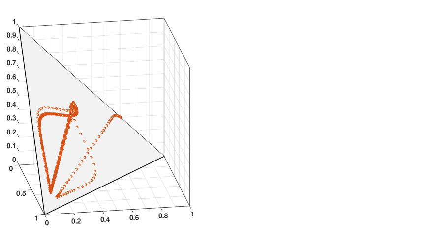
Figure 3: The evolution of the states of the constructed $\delta$-anti-passive game in feedback loop with the non-$\delta$-passive second order logit dynamics (9) projected into the simplex.

.

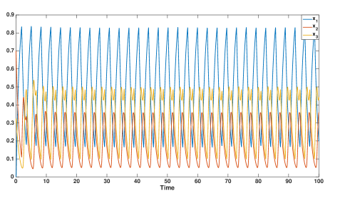
Figure 4: The evolution of the states of the constructed $\delta$-anti-passive game in feedback loop with the non-$\delta$-passive second order logit dynamics (9).

.

IV-B Replicator dynamics

Replicator dynamics are important class of evolutionary dynamics, which emerges originally from system biology and nature evolution [28]. It provides way to represent selection among a population of diverse types.

First, we show that first order replicator dynamics are indeed passive dynamics. In particular, replicator dynamics belongs to special class of passive systems known as lossless systems.

The replicator dynamics is given as follows:

$$\dot{x_{i}}=x_{i}(p_{i}-\sum_{j}x_{j}p_{j}),$$ (17)

where $p_{i}$ is the payoff for using strategy $i$.

Let $x^{*}$ to be a Nash equilibrium for the dynamic. Define $e_{x_{i}}=x_{i}-x^{*}_{i}$ to be the deviation from the equilibrium. The following theorem shows that first order replicator dynamics from the payoff $p_{i}$ to the error $e_{x_{i}}$ belongs to a special class of passive systems named lossless systems.

Theorem 4

Replicator dynamic mapping from $p_{i}$ to $e_{x_{i}}$ is passive lossless.

Proof:

Using $e_{x_{i}}=x_{i}-x^{*}_{i}$, the replicator dynamic equation (17) can be written as follows:

$$\dot{e}_{x_{i}}=(e_{x_{i}}+x^{*}_{i})(p_{i}-\sum_{j}(e_{x_{j}}+x^{*}_{j})p_{j}).$$ (18)

Define the following storage function,

$$V(e_{x})=-\sum_{i}x^{*}_{i}\ln\frac{e_{x_{i}}+x^{*}_{i}}{x^{*}_{i}}.$$ (19)

Note that $V(0)=0$, and

$$V(e_{x}) =-\sum_{i}x^{*}_{i}\ln\frac{e_{x_{i}}+x^{*}_{i}}{x^{*}_{i}}$$

$$\geq-\ln\sum_{i}x^{*}_{i}\frac{e_{x_{i}}+x^{*}_{i}}{x^{*}_{i}}$$

$$=\sum_{i}x_{i}=1,$$

i.e., $V(e_{x})\geq 0$.

Now, the derivative of the storage function is given as follows:

$$\dot{V}(e_{x}) =-\sum_{i}x^{*}_{i}\frac{1}{e_{x_{i}}+x^{*}_{i}}\dot{e}_{x_{i}}$$

$$=-\sum_{i}x^{*}_{i}(p_{i}-\sum_{j}(e_{x_{j}}+x^{*}_{j})p_{j})$$

$$=-\sum_{i}x^{*}_{i}p_{i}+\sum_{i}x^{*}_{i}(\sum_{j}e_{x_{j}}p_{j}+\sum_{j}x^{*}_{j}p_{j})$$

$$=-\sum_{i}x^{*}_{i}p_{i}+\sum_{j}e_{x_{j}}p_{j}+\sum_{j}x^{*}_{j}p_{j}$$

$$=\sum_{j}e_{x_{j}}p_{j}.$$

This implies that replicator dynamics is passive (lossless) system. ∎

It is known that replicator dynamics can exhibit different behaviors, that is stable, null stable and unstable depending on the game, (e.g., [11]). For example one can show that rock paper scissors game with replicator dynamics can generate these three different behaviors. These behaviors can be seen as a consequences of the lossless property of the replicator dynamics.

One can show that the linearization of the first order replicator dynamic results in a single integrator. Now, we will show that the second order replicators are non-passive dynamics, as the linearization result in double integrator (double poles at the origin). Hence, according to our result in this paper, it is possible to construct higher-order game that result in instability with the second order replicator dynamics.

The second order replicator dynamics can be obtained by introducing auxiliary state $\widehat{p}$ in the payoff function. This results in the following dynamics:

$$\dot{x_{i}} =x_{i}(\widehat{p}_{i}-\sum_{j}x_{j}\widehat{p}_{j})$$ (20a)

$$\dot{\widehat{p}_{i}} =p_{i}.$$ (20b)

The equilibrium conditions are $p_{i}^{*}=0$, $x_{i}^{*}=\sigma_{\text{max}}(\widehat{p}_{i}^{*})$, and $\widehat{p}_{i}^{*}=1$ .

The linearization of the replicator dynamics (20) is given as follows:

$$\delta\dot{x} =A\delta x+\beta\delta\widehat{p}$$

$$\delta\dot{\widehat{p}} =\delta p,$$

where, $A=\begin{bmatrix}-x_{1}^{*}&-x_{1}^{*}&\cdots&-x_{1}^{*}\\ -x_{2}^{*}&-x_{2}^{*}&\cdots&-x_{2}^{*}\\ \vdots&\vdots&\vdots&\vdots\\ -x_{n}^{*}&-x_{n}^{*}&\cdots&-x_{n}^{*}\end{bmatrix}$, $\beta=I-x^{*}x^{*T}$ and $x^{*}$ is any point in the simplex. The reduced system can be obtained using the transformation $\delta x=\delta x^{*}+N\delta w$, $\delta p=\delta p^{*}+N\delta q$ and $\delta\widehat{p}=N\xi$ as follows:

$$\delta\dot{w} =N^{T}AN\delta w+N^{T}\beta N\xi$$

$$\dot{\xi} =\delta q.$$

Now, consider the case where $n=3$ and $x_{i}^{*}=\frac{1}{3}$,

$$\begin{bmatrix}\delta\dot{w}\\ \dot{\xi}\end{bmatrix} =\begin{bmatrix}0&0&1&0\\ 0&0&0&1\\ 0&0&0&0\\ 0&0&0&0\end{bmatrix}\begin{bmatrix}\delta w\\ \xi\end{bmatrix}+\begin{bmatrix}0&0\\ 0&0\\ 1&0\\ 0&1\end{bmatrix}\delta q$$ (21a)

$$\delta y =\begin{bmatrix}1&0&0&0\\ 0&1&0&0\end{bmatrix}\begin{bmatrix}\delta w\\ \xi\end{bmatrix}.$$ (21b)

The system (21) is a double integrator, which is not passive. Accordingly, one can construct higher-order passive game that results in instability with the second order replicator dynamics. For instance, the higher-order game can be constructed as follows:

$$X =X^{*}+N\delta w$$

$$\dot{z} =\begin{bmatrix}-1&0\\ 0&-1\end{bmatrix}z+\begin{bmatrix}1&0\\ 0&1\end{bmatrix}\delta w$$

$$P =P^{*}+N\begin{bmatrix}-1&0\\ 0&-1\end{bmatrix}z.$$

Similarly, as in logit dynamics in the previous section, one can show that the above game $\delta$-anti-passive from strategies $X$ to payoff $P$.

Figs. 5 and 6 shows the evolution of the states of the positive feedback interconnection between the constructed game, which is $\delta$-anti-passive, and second order non-$\delta$-passive replicator dynamic (20).

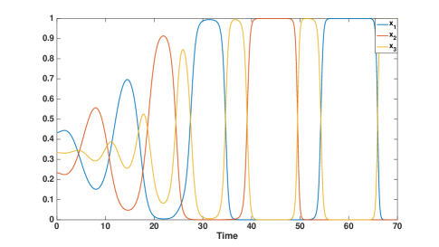
Figure 5: The evolution of the states of the constructed $\delta$-anti-passive game in feedback loop with the non-$\delta$-passive second order replicator dynamics (20).

.

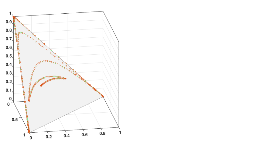
Figure 6: The evolution of the states of the constructed $\delta$-anti-passive game in feedback loop with the non-$\delta$-passive second order replicator dynamics (20) projected into the simplex.

.

V Concluding Remarks

In this paper, passivity analysis for higher order dynamics and games has been presented. The necessary conditions for evolutionary dynamics to exhibit stable behaviors for all higher-order passive games is provided. Methods from robust control analysis are used to show that if an evolutionary dynamic does not satisfy the passivity property, then it is possible to construct a higher-order passive game that results in unstable feedback loop. The results is employed to construct a higher-order passive games for two different dynamics to illustrate the feedback passivity concept in games.

One can conclude similar result (under some detailed conditions) for the nonlinear passive dynamics by constructing linear non-passive system that result in instability with the linearization of the nonlinear system. In other words, the following conjecture is true under some detailed conditions: Conjecture: If a nonlinear system is locally non-passive, i.e., the linearization around an equilibrium point $(x_{0},u_{0})$ is non-passive, then it is possible to construct a passive linear system that results in instability with the nonlinear system. This conjecture was illustrated in our discussion on higher-order dynamics and games.

Similar investigation for first order dynamics was conducted in [9]. They considered similar question raised in this paper, but for class of standard learning dynamics from passivity perspective. Implications of stability for various passive dynamics both analytically and by means of numerical simulations was discussed.

References

- [1] W. H. Sandholm, Population Games and Evolutionary Dynamics. MIT Press, 2010.
- [2] J. Hofbauer and K. Sigmund, Evolutionary Games and Population Dynamics. Cambridge, UK: Cambridge University Press, 1998.
- [3] H. P. Young, Individual Strategy and Social Structure. Princeton, NJ: Princeton University Press, 1998.
- [4] J. M. Smith, Evolution and the Theory of Games. Cambridge University Press, 1982.
- [5] J. Marden and J. S. Shamma, “Game theory and distributed control,” in Handbook of Game Theory, H. P. Young and S. Zamir, Eds. North-Holland, 2015, vol. 4, pp. 861–899.
- [6] D. Fudenberg and D. Levine, The Theory of Learning in Games. Cambridge, MA: MIT Press, 1998.
- [7] S. Hart, “Adaptive heuristics,” Econometrica, vol. 73, no. 5, pp. 1401–1430, 2005.
- [8] H. P. Young, Strategic Learning and its Limits. Oxford University Press, 2005.
- [9] S. Park, “Distributed estimation and stability of evolutionary game dynamics with applications to study of animal motions,” Ph.D. dissertation, University of Maryland, 2015.
- [10] J. Hofbauer and K. Sigmund, “Evolutionary game dynamics,” Bulletin of the American Mathematical Society, vol. 40, no. 4, pp. 479–519, 2003.
- [11] J. Hofbauer and W. H. Sandholm, “Stable games and their dynamics,” Journal of Economic Theory, vol. 144, no. 4, pp. 1665–1693, 2009.
- [12] S. Sato, E. Akiyama, and J. D. Farmer, “Chaos in learning a simple two person game,” Proceedings of the National Academy of Sciences, vol. 99, no. 7, pp. 4748–4751, 2002.
- [13] S. Hart and A. Mas-Colell, “Uncoupled dynamics do not lead to Nash equilibrium,” American Economic Review, vol. 93, no. 5, pp. 1830–1836, 2003.
- [14] D. Fudenberg and D. K. Levine, “Consistency and cautious fictitious play,” Journal of Economic Dynamics and Control, vol. 19, no. 5–7, pp. 1065–1089, 1995.
- [15] S. Hart and A. Mas-Colell, “A general class of adaptative strategies,” Journal of Economic Theory, vol. 98, no. 1, pp. 26–54, 2001.
- [16] M. J. Fox and J. S. Shamma, “Population games, stable games, and passivity,” Games, vol. 4, no. 4, pp. 561–583, 2013.
- [17] J. C. Willems, “Dissipative dynamical systems part I: General theory,” Archive for Rational Mechanics and Analysis, vol. 45, no. 5, pp. 321–351, 1972.
- [18] J. S. Shamma and G. Arslan, “Dynamic fictitious play, dynamic gradient play, and distributed convergence to nash equilibria,” IEEE Transactions on Automatic Control, vol. 50, no. 3, pp. 312–327, 2005.
- [19] G. Arslan and J. S. Shamma, “Anticipatory learning in general evolutionary games,” in 45th IEEE Conference on Decision and Control, San Diego, CA, December 2006, pp. 6289–6294.
- [20] R. Laraki and P. Mertikopoulos, “Higer order game dynamics,” Journal of Economic Theory, vol. 148, no. 6, pp. 2666–2695, 2013.
- [21] J. S. Shamma, “The necessity of the small-gain theorem for time-varying and nonlinear systems,” IEEE Transactions on Automatic Control, vol. 36, no. 10, pp. 1138–1147, 1991.
- [22] J. S. Shamma and R. Zhao, “Fading-memory feedback systems and robust stability,” Automatica, vol. 29, no. 1, pp. 191–200, 1993.
- [23] R. A. Freeman, “On the necessity of the small-gain theorem in the performance analysis of nonlinear systems,” in Proceedings of the 40th IEEE Conference on Decision and Control, Orlando, Florida, December 2001, pp. 51–56.
- [24] A. V. der Schaft, L2-Gain and Passivity Tecniques in Nonlinear Control. Springer Science & Business Media, 2012.
- [25] R. Lozano, B. Brogliato, O. Egeland, and B. Maschke, Dissipative Systems Analysis and Control: Theory and Applications. SpringerScience & Business Media, 2013.
- [26] K. Zhou, J. C. Doyle, and K. Glover, Robust and Optimal Control. Upper Saddle River, NJ: Prentice-Hall, Inc., 1996.
- [27] D. McFadden, “Conditional logit analysis of qualitative choice behavior,” Frontiers in Econometrics, pp. 105–142, 1974.
- [28] P. Schuster and K. Sigmund, “Replicator dynamics,” Journal of Theoretical Biology, vol. 100, no. 3, pp. 533–538, 1983.