On the RR Lyrae stars in globulars: IV. $\omega$ Centauri Optical UBVRI Photometry^*

Abstract

New accurate and homogeneous optical UBVRI photometry has been obtained for variable stars in the Galactic globular $\omega$ Cen (NGC 5139). We secured 8202 CCD images covering a time interval of 24 years and a sky area of 84$\times$48 arcmin. The current data were complemented with data available in the literature and provided new, homogeneous pulsation parameters (mean magnitudes, luminosity amplitudes, periods) for 187 candidate $\omega$ Cen RR Lyrae (RRLs). Among them we have 101 RRc (first overtone), 85 RRab (fundamental) and a single candidate RRd (double-mode) variables. Candidate Blazhko RRLs show periods and colors that are intermediate between RRc and RRab variables, suggesting that they are transitional objects. The comparison of the period distribution and of the Bailey diagram indicates that RRLs in $\omega$ Cen show a long-period tail not present in typical Oosterhoff II (OoII) globulars. The RRLs in dwarf spheroidals and in ultra faint dwarfs have properties between Oosterhoff intermediate and OoII clusters. Metallicity plays a key role in shaping the above evidence. These findings do not support the hypothesis that $\omega$ Cen is the core remnant of a spoiled dwarf galaxy. Using optical Period-Wesenheit relations that are reddening-free and minimally dependent on metallicity we find a mean distance to $\omega$ Cen of 13.71$\pm$0.08$\pm$0.01 mag (semi-empirical and theoretical calibrations). Finally, we invert the I-band Period-Luminosity-Metallicity relation to estimate individual RRLs metal abundances. The metallicity distribution agrees quite well with spectroscopic and photometric metallicity estimates available in the literature.

1 Introduction

The Galactic stellar system $\omega$ Cen lies at the crossroads of several open astrophysical problems. It is the most massive Milky Way globular cluster ($4.05\cdot 10^{6}M_{\odot}[d/(5.5\pm 0.2{\rm\,kpc})]^{3}$ where d is the distance, D’Souza & Rix, 2013) and was the first to show a clear and well defined spread in metal-abundance (Norris & Da Costa, 1995; Johnson & Pilachowski, 2010) in $\alpha$ and in s- and r-process elements (Johnson et al., 2009). On the basis of the above peculiarities it has also been suggested that $\omega$ Cen and a few other massive Galactic Globular Clusters (GGCs) might have been the cores of pristine dwarf galaxies (Da Costa & Coleman, 2008; Marconi et al., 2014).

The distance to $\omega$ Cen has been estimated using primary and geometrical distance indicators. The Tip of the Red Giant Branch (TRGB) was adopted by Bellazzini et al. (2004); Bono et al. (2008b) with distances ranging from 13.65 to 13.70 mag. The K-band Period-Luminosity (PL) relations of RR Lyrae stars (RRLs) have been adopted by Longmore et al. (1990); Sollima et al. (2006b); Bono et al. (2008b). The distance moduli they estimated range from 13.61 to 13.75 mag. On the other hand, $\omega$ Cen distance moduli based on the relations between luminosity and iron abundance for RRLs range from 13.62 to 13.72 mag (Del Principe et al., 2006). The difference in distance between the different methods is mainly due to the intrinsic spread in the adopted diagnostics and in the reddening correction.

Optical PL relations for SX Phoenicis stars were adopted by McNamara (2011) who found a distance of 13.62$\pm$0.05 mag. One eclipsing variable has been studied by Kaluzny et al. (2007), and they found a distance modulus of 13.49$\pm$0.14 mag and 13.51$\pm$0.12 mag for the two components. The key advantage in dealing with eclipsing binaries is that they provide very accurate geometrical distances (Pietrzyński et al., 2013). Estimates based on cluster proper motions provide distance estimates that are systematically smaller than obtained from the other most popular distance indicators (13.27 mag, van Leeuwen et al. (2000); 13.31$\pm$0.04 mag, Watkins et al. (2013)). The reasons for this difference are not clear yet.

The modest distance and the large mass of $\omega$ Cen make this stellar system a fundamental laboratory to constrain evolutionary and pulsation properties of old (t>10 Gyr) low-mass stars. The key advantage in dealing with stellar populations in this stellar system is that they cover a broad range in metallicity (–2.0$\lesssim$ [Fe/H] $\lesssim$–0.5, Pancino et al. (2002); –2.5$\lesssim$ [Fe/H] $\lesssim$+0.5, Calamida et al. (2009); –2.2$\lesssim$ [Fe/H] $\lesssim$–0.6, Johnson & Pilachowski (2010)) and they are located at the same distance (Castellani et al., 2007). Moreover, the high total stellar mass does provide the opportunity to trace fast evolutionary phases (Monelli et al., 2005; Calamida et al., 2008) together with exotic (Randall et al., 2011) and/or compact objects (Bono et al., 2003b).

Exactly for the same reasons mentioned before $\omega$ Cen was a crucial crossroads for RRLs. The first detailed investigation of RRLs was provided more than one century ago in a seminal investigation by Bailey (1902). Using a large set of photographic plates he identified and characterized by eye 128 RRLs, providing periods, amplitudes and a detailed investigation of the shapes of the light curves. In particular, he suggested the presence of three different kind of pulsating variables (RRa, RRb, RRc) in which the luminosity variation amplitude steadily decreases and the shape of the light curve changes from sawtooth to sinusoidal. This investigation was supplemented more than thirty years later by Martin (1938) on the basis of more than 400 photographic plates collected by H. van Gent on a time interval of almost four years and measured with a microdensitomer. He provided homogeneous photometry and very accurate periods for 136 RRL variables.

We needed to wait another half century to have a detailed and almost complete census of RRL in $\omega$ Cen based on CCD photometry, by the OGLE project (Kaluzny et al., 1997, 2004). They collected a large number of CCD images in V and B covering a time interval of three years (Kaluzny et al., 1997) and one and half years (Kaluzny et al., 2004) and provided a detailed analysis of the occurrence of the Blazhko effect (a modulation of the light amplitude on time scales from tens of days to years, Blažko, 1907). A similar analysis was also performed by Weldrake et al. (2007) using the observing facility and photometric system of the MACHO project. They collected 875 optical images covering a period of 25 days.

A detailed near-infrared (NIR) analysis was performed by Del Principe et al. (2006) using time series data collected with SOFI at NTT. They provided homogeneous JK_s photometry for 180 variables and provided a new estimate of the $\omega$ Cen distance modulus using the K-band PL relation (13.77$\pm$0.07 mag). A similar analysis was recently performed by Navarrete et al. (2015) based on a large set of images collected with the VISTA telescope. They provided homogeneous JK_s photometry for 189 probable member RRLs (101 RRc, 88 RRab) and discussed the pulsation properties of the entire sample in the NIR. In particular, they provided new NIR reference lines for Oosterhoff I (OoI) and Oosterhoff II (OoII) clusters. Moreover, they further supported the evidence that RRab in $\omega$ Cen display properties similar to OoII systems. These investigations have been complemented with a detailed optical investigation covering a sky area of more than 50 square degrees by Fernández-Trincado et al. (2015a). They detected 48 RRLs and the bulk of them (38) are located outside the tidal radius. However, detailed simulations of the different Galactic components and radial velocities for a sub-sample of RRLs indicate a lack of tidal debris around the cluster.

This is the fourth paper of a series focussed on homogeneous optical, near-infrared, and mid-infrared photometry of cluster RRLs. The structure of the paper is as follows. In § 2 we present the optical multi-band UBVRI photometry that we collected for this experiment together with the approach adopted to perform the photometry on individual images and on the entire dataset. In subsection 3.1 we discuss in detail the identification of RRLs and the photometry we collected from the literature to provide homogeneous estimates of the RRL pulsation parameters. Subsection 3.2 deals with the period distribution, while subsection 3.3 discusses the light curves and the approach we adopted to estimate the mean magnitudes and the luminosity variation amplitudes. The Bailey diagram (luminosity variation amplitude vs period) is discussed in § 3.4, while the amplitude ratios are considered in § 3.5. Section 4 is focussed on the distribution of RRLs in the color-magnitude diagram (CMD) and on the topology of the instability strip. In § 5 we perform a detailed comparison of the period distribution and the Bailey diagram of $\omega$ Cen RRLs with the similar distributions in nearby gas-poor systems (globulars, dwarf galaxies). Section 6 deals with RRL diagnostics, namely the PL and the Period-Wesenheit (PW) relation, while in § 7 we discuss the new distance determinations to $\omega$ Cen based on optical PW relations. Section 8 deals with the metallicity distribution of the RRLs, based on the I-band PL relation, and the comparison with photometric and spectroscopic estimates available in the literature. Finally, § 9 gives a summary of the current results together with a few remarks concerning the future of this project.

2 Optical photometry

We provide new accurate and homogeneous calibrated multi-band UBVRI photometry for the candidate RRLs in $\omega$ Cen. The sky area covered by our calibrated photometry is roughly 57 $\mkern-4.0mu{}^{\prime}$$\times$56 $\mkern-4.0mu{}^{\prime}$around the cluster center (see the end of this section). We acquired 8202 optical CCD images of $\omega$ Cen from proprietary datasets (6211 images, 76%) and public archives and extracted astrometric and photometric measurements from them using well established techniques (see, e.g., Stetson, 2000, 2005, and references therein). Among these we were able to photometrically calibrate 7766 images (including 320 U-, 2632 B-, 3588 V-, 339 R-, and 887 I-band images) covering a time interval of slightly over 24 years. Table 1 gives the log of observations and a detailed description of the different optical datasets adopted in this investigation. Note that the largest datasets are danish95 (1786 CCD images) and danish98 (1981 CCD images). The danish99 dataset also includes a sizable number of exposures (632 CCD images), but they were collected on two nights separated by seven days. For this reason, the danish99 dataset is very useful to have a guess of the shape of the light curve, but the period determinations based on this dataset in isolation are not as accurate as those based on datasets covering a larger time interval. The B-band photometry based on danish95 and on danish98 images is less accurate when compared with the other datasets. The danish98 dataset showed large variations of the photometric zero-point with position on the chip. The large number of local standards allowed us to take account for this positional effect. The photometry based on all the other datasets was labeled other and provides most of the time interval covered by our photometric catalog. Note that these data were collected with several ground-based telescopes available at CTIO (0.9m, 1.5m, Blanco 4m), ESO (0.9m, MPI/ESO 2.2m, NTT, VLT), and SAAO (1m). In passing we also note that the current dataset was also built up to detect fast evolving objects, i.e., objects experiencing evolutionary changes on relatively short time scales.

The defining of local standards in the field of $\omega$ Cen was performed following the same criteria discussed in our previous work on M4 (free from blending, a minimum of three observations, standard error lower than 0.04 mag and intrinsic variability smaller than 0.05 mag, Stetson et al., 2014a). As a whole 4,180 stars satisfy these requirements and 4,112 of these have high-quality photometry (at least five observations, standard error $<$ 0.02 mag and intrinsic variability smaller than 0.05 mag) in at least two bands: 3,462 in U, 4,112 in B, 4,106 in V, 875 in R, and 3,445 in I.

These stars have been used as a local reference for the photometric calibration of 847,138 stars in the field of $\omega$ Cen from the final ALLFRAME reduction (Stetson, 1994). The median seeing of the different datasets is 1.2^′′, but our 25-th percentile is 0.86^′′, and the 10-th percentile is 0.65^′′. We measured stars in up to 2,000 images covering the innermost cluster regions (13.4^′$\times$13.5^′); this means that the stars located there, were observed in $\sim$200 images with seeing better than 0.65^′′. The cluster regions in which we measured stars in up to 100 images is 36.6^′$\times$31.6^′; this means that roughly ten images were collected with a seeing better than 0.65^′′. The use of ALLFRAME means that detections visible in these images and their positions were also used to fit those same stars in the poorer-seeing images. This analysis resulted in 583,669 stars with calibrated photometry in all three of B, V, and I; 202,239 of them had calibrated photometry in all five of U, B, V, R, and I. A more detailed analysis of the current multiband photometric dataset will be provided in a forthcoming paper (Braga et al. 2016, in preparation).

The astrometry of our photometric catalog is on the system of the USNO A2.0 catalog (Monet et al., 1998). The astrometric accuracy is 0.1^′′and allows us to provide a very accurate estimate of $\omega$ Cen’s centroid. Following the approach applied to Fornax by Stetson et al. (1998b) we found $\alpha_{center}$ = 13^h 26^m 46.71^s, $\delta_{center}$ = –47^∘28 $\mkern-4.0mu{}^{\prime}$59^′′.9. The stars adopted to estimate the position of the cluster center have V-band magnitude between 16 and 20 and are located (with varying weights) up to $\sim$14 $\mkern-4.0mu{}^{\prime}$ from the adopted center. The mean epoch associated to these coordinates is May 2004. New and accurate structural parameters will be provided in a forthcoming paper.

3 RR Lyrae stars

3.1 Identification

We adopted the online reference catalog for cluster variables “Catalogue of Variable Stars in Globular Clusters” by C. Clement (Clement et al., 2001, updated 2015). This catalog lists 456 variables (197 candidate RRLs) within the truncation radius ($r_{t}$=57.03 arcmin, Harris, 1996) of $\omega$ Cen and it is mostly based on the detailed investigations of Kaluzny et al. (2004). This catalog was supplemented with more recent discoveries by Weldrake et al. (2007) and Navarrete et al. (2015). Two candidate field RRLs NV457 and NV458 discovered by Navarrete et al. (2015) were not included in the online catalog. To provide accurate and homogeneous photometry for the entire sample of RRLs along the line of sight of $\omega$ Cen, they were included in the current sample. We have also removed the field star V180 from the sample, following Navarrete et al. (2015) that classify it as a W UMa binary star on the basis of its color and pulsation amplitude. Finally, we have included V175, recently recognized as a field RRL by Fernández-Trincado et al. (2015a), that updated the uncertain classification of this object by Wilkens (1965). We ended up with 199 candidate RRLs. Eight out of the 199 objects are, according to their mean magnitudes and proper motions, candidate field stars (van Leeuwen et al., 2000; Navarrete et al., 2015). Note that we also included two variables with periods similar to RRLs but for which the classification is not well established, namely NV366 (Kaluzny et al., 2004) and the candidate field variable NV433 (Weldrake et al., 2007).

To overcome possible observational biases in the current RRL sample, the identification of variable stars was performed ab initio using the Welch-Stetson (WS, Welch & Stetson, 1993; Stetson, 1996) index. We adopted our own photometric catalog and we identified 176 candidate RRLs they had a WS index larger than 1.1. This list was cross matched with the Clement’s catalog and we found that all of them were already known. We have then compared the individual coordinates based on our astrometric solution with the ones given in the literature and we found that the median difference of the coordinates is 0^′′.41, with a standard deviation from the median of 0^′′.26. The difference for the entire sample is smaller than 2^′′; only for six out of the 176 stars is the difference between 1^′′and 2^′′.

The above data were supplemented with unpublished Walraven WULBV photometry for two RRLs—V55 and V84—collected by J. Lub in 1980-1981 at the Dutch telescope in La Silla. The Walraven photometry was transformed into the standard Johnson-Kron-Cousins photometric system (UBV) using the transformations provided by Brand & Wouterloot (1988). Moreover, we supplemented the photometry of the two variables observed by J. Lub with UBV photoelectric photometry from Sturch (1978). The number of RRLs for which we provide new astrometry is 186, while those for which we provide new photometry is 178.

For nine out of the remaining 21 stars, we were able to recover optical photometry in the literature: a)—V281 and V283 from OGLE (V band, Kaluzny et al., 1997); b)—V80, V177, NV411 and NV433 (V+R band, Weldrake et al., 2007); c)—V172, NV457 and NV458 from CATALINA (V band, Drake et al., 2009, 2013a, 2013b, 2014; Torrealba et al., 2015).

We performed detailed tests concerning the photometric zero-point using the objects in common and we found that there is no difference, within the photometric errors, between the current photometry and the photometry provided by OGLE, CATALINA, Sturch (1978) and by J. Lub. On the other hand, we have not been able to transform into the standard photometric system the photometry collected by Weldrake et al. (2007) for the four variables V80, V177, NV411 and NV433. For these four objects we only provided a homogeneous period determination, while the other five were fully characterized (period, mean magnitude, amplitude).

The positions of $\omega$ Cen RRLs based on our astrometric solution are listed in columns 2 and 3 of Table 2, together with their literature and current pulsation period (columns 4 and 5 in Table 2). The epoch of the mean magnitude along the rising branch (Inno et al., 2015) and of the maximum light are listed in column 6 to 9 of Table 2 together with the photometric band adopted for the measurements. Note that the above epochs have been estimated using the spline fits of the light curves discussed in Section 3.3.

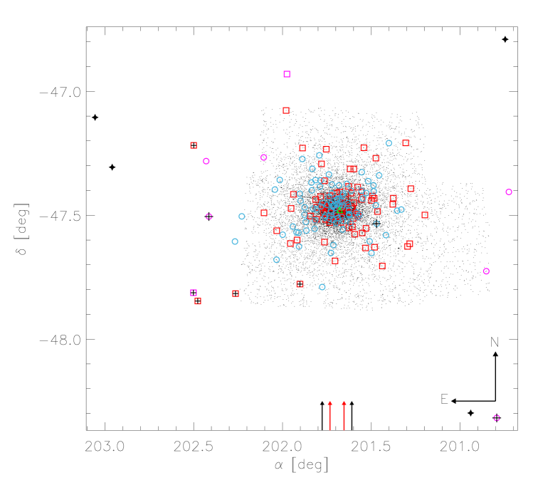
Figure 1: Spatial distribution of the entire sample of $\omega$ Cen RRLs (199). The current optical photometry covers a sky area of $\approx$25 $\mkern-4.0mu{}^{\prime}$across the cluster center. The upward red and black arrows plotted on the right ascension axis display the core and the half-mass radius (Harris, 1996). The black arrows plotted in the bottom right corner display the orientation. The squares and open circles display the position of RRab (90) and RRc (104) variables, respectively. The candidate RRd variable (V142) is marked with a green triangle. Magenta squares (RRab) and circles (RRc) mark the position of the eight variables for which we have retrieved periods and either optical or NIR mean magnitudes in the literature and for which a mode classification is possible. Black stars mark the position of the four variables for which we do not have solid pulsation paramter estimates and mode classification. The pluses mark the position of the eight candidate field RRLs.

The sky distribution of the 187 candidate RRLs for which we have estimated pulsation parameters is shown in Fig. 1, where red squares and light blue circles mark the position of fundamental (RRab) and first-overtone (RRc) RRLs (see §3.2). The candidate RRd variable V142 (see notes on individual variables in the Appendix) is marked with a green triangle.

We retrieved mean optical magnitude and periods from the literature for three variables: V151 (Martin, 1938), V159 (van Gent, 1948) and for V175 (Fernández-Trincado et al., 2015a). Mean NIR magnitudes and periods for five variables (V173, V181, V183, V455, V456) were retrieved from Navarrete et al. (2015). Magenta squares (RRab) and circles (RRc) mark the position of these eight variables. The four candidate variables identified by Wilkens (1965, V171, V178, V179) and by Sawyer Hogg (1973, V182) for which we do not have solid estimates of the pulsation parameters and mode classification are marked with black stars. Among the 195 RRLs for which the pulsation characterization has been performed we have 104 RRc, 90 RRab and a single RRd variable.

We performed a number of statistical tests concerning the radial distribution of RRab and RRc, but no clear difference was found.

3.2 Period distribution

To take full advantage of the observing strategy adopted to collect the time series we used two independent methods to determine the periods: the string method (Stetson, 1996; Stetson et al., 1998a) and our variant of the Lomb-Scargle (LS) method (Scargle, 1982). The key advantages of these methods are: a) they use multi-band photometry simultaneously; b) they take account for intrinsic photometric errors. We have checked that, within 0.002 days, period estimates based on the two methods agree quite well with each other. The periods based on the Lomb-Scargle method also agree with those given in the Clement catalog. The difference between the Lomb-Scargle and the Clement periods is typically smaller than 0.0001 days. Only 28 variables show a difference larger than 0.0001 days, but none has a difference larger than 0.001 days. Table 2 only gives the periods based on the Lomb-Scargle method, because this method was also used for the variables with photometry only available in the literature. A preliminary analysis on the uncertainties of the periods suggests us that they cannot be larger than $1\cdot 10^{-6}$ days.

The period derivatives of RRLs in $\omega$ Cen have been investigated by Jurcsik et al. (2001). They collected photometric data available in the literature covering more than one century. They found that a sizable sample of RRab display a steady increase in their period, thus supporting the redward evolution predicted by Horizontal Branch (HB) models (Bono et al., 2016). On the other hand, the RRc showed irregular trends in period changes. This indicates that period changes are affected by evolutionary effects and by other physical mechanisms that have not been fully constrained (Renzini & Sweigart, 1980). We plan to provide more quantitative constraints of the period changes after the analysis of NIR images we have already collected, since they will allow us to further increase the time interval covered by our homogeneous photometry.

It is well known that $\omega$ Cen hosts a sizable sample of RRc with periods longer than 0.4 days (Kaluzny et al., 2004). To constrain the pulsation mode of the candidate RRLs, we need to take account of their distribution in the Bailey diagram (period vs luminosity variation amplitude, see Section 3.4).

The current data allowed us to confirm the pulsation mode of the current candidate RRLs; they are listed in the last column of Table 3. Using either optical or NIR mean magnitudes (see §3.1) as a selection criterion to discriminate between candidate field and cluster RRLs, we found that the candidate cluster RRLs number 187, and among them 101 are RRc, 85 are RRab and one single candidate RRd variable.

To make the separation between field and cluster stars more clear the former in Fig. 1 were marked with a plus sign. As expected, field candidates tend to be located between the half-mass radius ($r_{h}=$ 5 arcmin, Harris, 1996) and the tidal radius ($r_{t}=$ 1.2 degrees, Marconi et al., 2014) of the cluster.

Note that, according to Weldrake et al. (2007) and to Navarrete et al. (2015), the classification of the variable NV433, that has a peculiar light curve, is unclear. However, its apparent magnitude (K$\sim$14.151 mag Navarrete et al., 2015) seems to suggest that it is a candidate field variable.

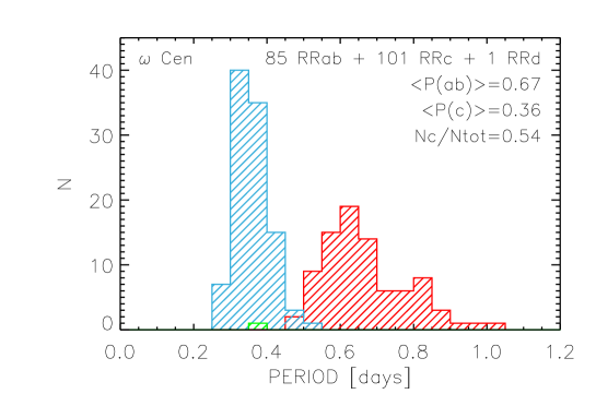
Figure 2: Period distribution for RRab (red) and RRc (light blue) RRLs in $\omega$ Cen. The candidate RRd variable (V142) is plotted in green. The number of RRab, RRc and RRd candidate RRLs are labeled together with the mean periods of RRab and RRc and the ratio between the number of RRc and the total number of RRLs ($N_{c}$/$N_{ab}+N_{d}+N_{c}$). See text for more details.

The period distribution plotted in Fig. 2 shows—as expected—a prominent peak for RRc (light blue shaded area) with roughly 20% of the variables (18 out of 101) with periods longer than 0.4 days.

The RRab show a broad period distribution ranging from 0.47 days to roughly one day (red shaded area). Long-period (P$\geq$0.82–0.85 days) RRLs are quite rare in Galactic globulars. Several of them have also been identified in two peculiar Bulge metal-rich globulars—NGC 6388, NGC 6441 (Pritzl et al., 2001, 2002)—and in the Galactic field (Wallerstein et al., 2009). Whether they are truly long-period RRLs or short-period Type II Cepheids (TIICs) is still a matter of lively debate (Soszyński et al., 2011; Marconi et al., 2011). In the current investigation we are assuming, following the OGLE team, that the transition between RRLs and TIICs takes place across one day. More quantitative constraints on this relevant issue will be addressed in a future paper.

The ratio between the number of RRc and the total number of RRL ($N_{tot}$=$N_{ab}$+$N_{d}$+$N_{c}$) is quite large ($N_{c}$/$N_{tot}=0.54$), roughly $\sim$0.1 larger than the typical ratio of Oosterhoff II (OoII) clusters: $N_{c}$/$N_{tot}\sim 0.44$, while the same ratio in Oosterhoff I (OoI) clusters is $N_{c}$/$N_{tot}\sim 0.29$ Oosterhoff (1939); Castellani & Quarta (1987); Caputo (1990). The mean Fundamental (F) period is $<P_{ab}>=0.668$ days, i.e., quite similar to OoII clusters, since they have $<P_{ab}>\sim 0.651$ days, while OoI clusters have $<P_{ab}>\sim 0.557$ days. The mean First Overtone (FO) period is $<P_{c}>=0.359$ days, once again similar to OoII clusters, since they have $<P_{c}>=0.356$ days, while OoI clusters have $<P_{c}>=0.312$ days. However, these mean parameters should be treated with caution, since they have been estimated using the same selection criteria adopted by Fiorentino et al. (2015), i.e., we only took into account GCs hosting at least 35 RRLs. A more detailed comparison with different Oosterhoff groups and with RRLs in nearby stellar systems is given in Section 5.

3.3 Light curves

The observing strategy of the large optical datasets adopted in this investigation was focussed on RRLs. The main aim was an extensive and homogeneous characterization of their pulsation properties (period, mean magnitudes, amplitudes and epochs of minimum and maximum light). The time coverage (24 years) and the approach adopted to perform simultaneous multiband photometry allow us to provide very accurate period determinations (see Section 3.2).

This experiment was also designed to provide accurate estimates of period variations, but this topic will be addressed in a forthcoming paper. This is the reason why we collected a few hundred phase points in a single band on individual nights. More importantly, we collected more than one thousand phase points on a time interval of one to two weeks. As a whole, this extremely dense sampling provides us very good phase coverage for both short and long-period RRLs. However, the phase coverage is marginally affected by alias in the transition between RRL and short-period TIIC (BL Herculis), i.e., in the period range across $\sim$1.0 day.

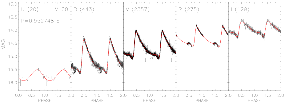
Figure 3: From left to right UBVRI light curves of the RRab variable V100. Red lines show the spline fits adopted to calculate mean magnitudes, luminosity variation amplitudes and the epochs of mean magnitude and maximum light. Data and analytical fits cover two full pulsation cycles. The number of phase points per band are displayed in parentheses. The period is also labeled. The vertical error bars display intrinsic errors of individual data points.

The results of this observing strategy are visible in Figures 3, 4 and 5 that show, from left to right, a selection of optical light curves in the UBVRI bands for a RRL star pulsating in the F mode (V100), in the FO mode (V103) and a RRab variable affected by Blazhko (V120). The number of phase points per band and the period are also labelled. The vertical bars display individual photometric errors. They are of the order of $\sigma_{U}\sim$0.026, $\sigma_{B}\sim$0.025, $\sigma_{V}\sim$0.014, $\sigma_{R}\sim$0.012 and $\sigma_{I}\sim$0.035.

Solid red lines in Figures  3, 4 and 5 show the spline fits that we adopted to derive mean magnitudes, amplitudes and epochs of mean and maximum light of RRLs. The UBVRI mean magnitudes of the candidate RRLs were derived by intensity-averaging the spline fits over a full pulsation cycle. They are listed in columns 2 to 6 of Table 3. The column 12 of the same table gives the photometric quality index of the individual light curves in the different bands. It is zero for no phase coverage, one for poor phase coverage, two for decent coverage and three for good phase coverage. The errors of the mean magnitudes have been determined as the weighted standard deviation between the spline fit and the individual phase points. We found that the errors on average, for good quality light curves, are: $\sigma_{B}=0.02$ mag, $\sigma_{V}=0.01$ mag, $\sigma_{R}=0.01$ mag and $\sigma_{I}=0.03$ mag. The same errors for decent quality light curves are: $\sigma_{U}=0.02$ mag, $\sigma_{B}=0.02$ mag, $\sigma_{V}=0.01$ mag, $\sigma_{R}=0.02$ mag and $\sigma_{I}=0.04$ mag. The mean magnitudes of the objects for which the light curve coverage is poor, typically in the U-band, was estimated as the median of the measurements and their errors range from 0.04 (I band) to 0.11 mag (U band). The luminosity variation amplitudes in the UBVRI bands of the candidate RRLs for which we have either our photometry or literature photometry have been estimated as the difference between the minimum and the maximum of the spline fit. They are listed in columns 7 to 11 of Table 3. Note that the U-band amplitudes are available only for a limited number of variables. Moreover, the minimum and maximum amplitudes of the candidate Blazhko RRLs and of the candidate RRd variable were estimated as the amplitudes of the lower and the upper envelope of the observed data points.

3.4 Bailey diagram

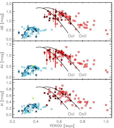
Figure 6: Top: Bailey diagram, B-band amplitude versus period, for candidate $\omega$ Cen RRLs. RRab and RRc stars are plotted as red squares and light blue open circles, respectively. The candidate RRd variable (V142) is marked with a green triangle. Its abscissa is fixed at the period of the main (FO) mode. Candidate Blazhko RRLs are marked with a black cross. The solid black lines overplotted on the RRab stars display the loci typical of OoI and OoII GCs (Cacciari et al., 2005). The solid black lines overplotted on the RRab stars display the loci typical of OoI and OoII GCs (Cacciari et al., 2005). The solid black line overplotted on the RRc stars shows the locus of RRc typical of OoII GCs (Kunder et al., 2013b). Note that the latter relation was originally provided by Kunder et al. (2013b) for the V-band. It was transformed into the B-band using $AB/AV$=1.26. Middle: Same as the top, but for the V-band amplitude. The vertical red bars display the range in luminosity amplitude of candidate Blazhko RRLs. The Oosterhoff relations for RRab stars were originally provided by (Cacciari et al., 2005) for the B-band. They were transformed into the V-band using $AB/AV$=1.25. Bottom: Same as the top, but for the I-band amplitude. The original Oosterhoff relations for RRc and RRab stars were transformed into the I-band using $AI/AV$=0.63 (see § 3.5).

The Bailey diagram—period vs luminosity variation amplitude—is a powerful diagnostic for variable stars, being reddening- and distance-independent (Smith et al., 2011). Moreover, the luminosity variation amplitudes are also minimally affected by possible uncertainties in the absolute photometric zero-point. These advantages become even more compelling when dealing with large cluster samples, and indeed, $\omega$ Cen RRL provides the largest cluster sample after M3 and M62. The data in Fig. 6 show, from top to bottom the amplitudes in B, V and I band. The two solid lines overplotted on the RRab variables display the analytical relations for OoI and OoII clusters derived by Cacciari et al. (2005), while the solid line plotted over the RRc variables is the analytical relation for OoII clusters derived by (Kunder et al., 2013b).

The majority of the RRab of $\omega$ Cen lie along the OoII locus for periods longer than $\sim$0.6 days, and along the OoI locus for shorter periods. On the other hand, RRab with periods longer than 0.80 days show, at fixed period, amplitudes that are systematically larger than typical for OoII clusters. Moreover, they also display a long-period tail not present in typical OoII clusters. The same distribution has already been observed in the $V$-band Bailey diagram provided by Clement & Rowe (2000); Kaluzny et al. (2004). More interestingly, there is evidence that a significant fraction (79%) of candidate Blazhko RRLs (22 out of 28) have periods shorter than 0.6 days. This finding further supports the evidence originally brought forward by Smith (1981) concerning the lack of Blazhko RRLs with a period longer than $\approx$0.7 days. Note that the Blazhkocity (Kunder et al., 2013b) among the RRab of $\omega$ Cen with periods shorter than 0.6 days is of the order of 46%, thus suggesting that $\omega$ Cen is a cluster with a Blazhkocity that is on average 50% larger than other GGCs. However, this finding could be the consequence that time series data of GGCs do not cover with the appropriate cadence large time intervals (Jurcsik et al., 2012).

The above findings together with similar empirical evidence concerning the precise position of RRd variables (Coppola et al., 2015) sheds new light on the topology of the RRL instability strip, and in particular, on the color/effective temperature range covered by the different kind of pulsators.

The RRc (light blue squares) plotted in Fig. 6 display the typical either "hairpin" or "bell" shape distribution. The OoII sequence from Kunder et al. (2013b) appears to be, at fixed pulsation period, the upper envelope of the RRc distribution. Moreover, they seem to belong to two different sub-groups (if we exclude a few long- and short-period outliers): a) short-period—with periods ranging from $\sim$0.30 to $\sim$0.36 days and visual amplitudes ranging from a few hundredths of a magnitude to a few tenths; b) long-period—with periods ranging from $\sim$0.36 to $\sim$0.45 days and amplitudes clustering around $AV\sim$0.5 mag. With the only exception of the metal-rich clusters NGC 6388 (Pritzl et al., 2002) and NGC 6441 (Pritzl et al., 2001), and with V70 in M3 (Jurcsik et al., 2012), $\omega$ Cen is the only GGC where long-period RRc are found (Catelan, 2004b). Theoretical and empirical evidence indicates that the RRc period distribution is affected by metallicity (Dall’Ora et al., 2003). An increase in metal content causes a steady decrease in the pulsation period (Bono et al., 1997b). The above evidence seems to suggest that the dichotomous distribution of RRc might be the consequence of a clumpy distribution in metal abundance (see Section 8). The reader interested in detailed insights on the metallicity dependence of the RRLs position in the Bailey diagram is referred to Navarrete et al. (2015).

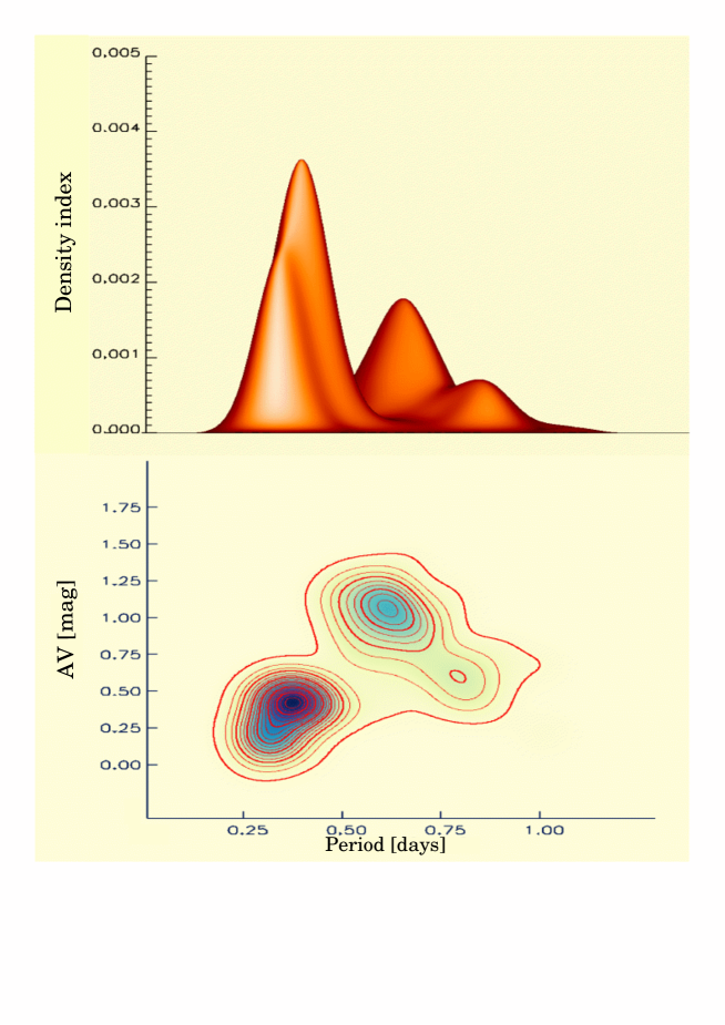
Figure 7: Top: 3D Bailey diagram for candidate $\omega$ Cen RRLs: pulsation period in days, V-band amplitude and the Z-axis in arbitrary units. Bottom: Same as the top, but the view is from the top.

To further constrain the fine structure of the Bailey diagram we plotted the same variables in a 3D plot. The distribution was smoothed with a Gaussian kernel. The top panel of Fig. 7 shows that the distribution is far from being homogeneous, and indeed, both the RRc and the RRab variables show double secondary peaks in the shorter and in the longer period range, respectively. This evidence is further supported by the iso-contours plotted in the bottom panel of the same figure. The iso-contours were estimated running a Gaussian kernel, with unit weight, over the entire sample. In this panel the long-period of RRab variables can also be easily identified.

Despite the fact that the Bailey diagram for $\omega$ Cen RRL shows some peculiarities, these results fully support the OoII classification for $\omega$ Cen RRL suggested by Clement & Rowe (2000) and more recently by Navarrete et al. (2015).

3.5 Luminosity amplitude ratio

The amplitude ratios are fundamental parameters together with the periods and the epoch of a reference phase (luminosity maximum, mean magnitude) for estimating the mean magnitude of variable stars using template light curves. This approach provides mean magnitudes with a precision of a few hundredths of a magnitude from just a few phase points (Jones et al., 1996; Soszyński et al., 2005; Inno et al., 2015). Two key issues that need to be addressed in using the amplitude ratios are possible differences between RRab and RRc variables and the metallicity dependence (Inno et al., 2015). The $\omega$ Cen RRLs play a key role in this context, for both the sample size and the well known spread in iron abundance.

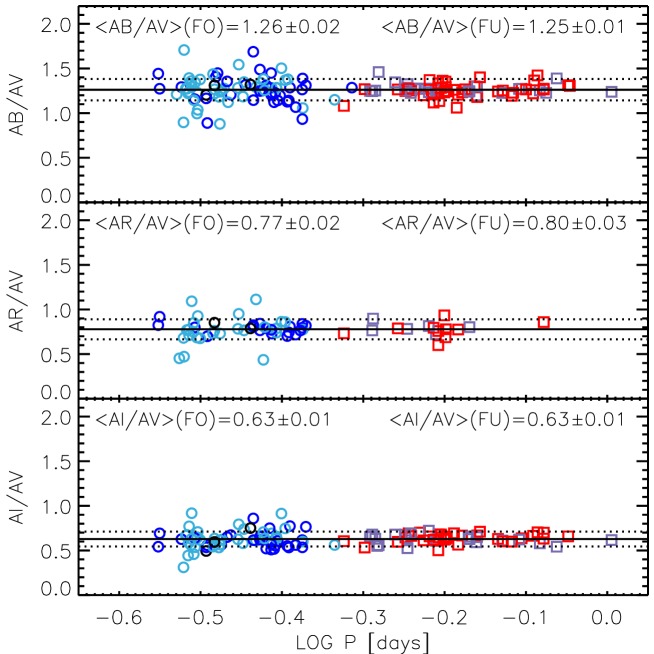
Figure 8: Top: Ratio between the B- and the V-band amplitude versus the pulsation period for candidate $\omega$ Cen RRLs. Metal-poor and metal-rich variables (threshold at [Fe/H] = –1.7) are shown with different colors. Light blue and red symbols display metal-poor RRc and RRab, while blue and violet symbols mark metal-rich RRc and RRab, respectively. Black symbols are for variables with no [Fe/H] estimate. The iron abundances come from R00 and S06 and the adopted values are listed in column 4 of Table 10 (see text for more details concerning iron abundances). The average value of the amplitude ratio for RRab and RRc and the error on the mean are also labeled. The solid line shows the mean value of the global sample (All), while the dashed lines display the standard deviation. Middle: Same as the top, but for the amplitude ratio between R- and V-band. Bottom: Same as the top, but for the amplitude ratio between I- and V-band.

Following the same approach adopted by Kunder et al. (2013b) and Stetson et al. (2014a), we estimated the amplitude ratios in different bands. Fig. 8 shows the mean values of the amplitude ratios: $AB$/$AV$ (top), $AR$/$AV$ (middle) and $AI$/$AV$ (bottom) of $\omega$ Cen RRLs. We included only variables with the best-sampled light curves. We have quantified the goodness of the sampling of the light curve with a quality parameter, based on the number of phase points, the presence of phase gaps and the uncertainties in the magnitudes of the individual phase points. The paucity of RRab variables in the middle panel is due to the fact that our R-band photometry was mostly collected during two single nights. Therefore, the R-band light curves of long-period RRLs are not well-sampled.

The amplitude ratios were estimated using the bi-weight to remove the outliers (Beers et al., 1990; Fabrizio et al., 2011; Braga et al., 2015). The individual values for RRab, RRc and for the global (All) samples are listed in Table 4 together with their errors and standard deviations. The errors account for the uncertainty in the photometry and in the estimate of luminosity maxima and minima. Estimates listed in Table 4 and plotted in Fig. 8 indicate that there is no difference, within the errors, between the RRab and RRc amplitude ratios. Moreover, the data in Fig. 8 show no clear dependence on the metal content: indeed metal-rich ([Fe/H] > –1.70, blue and violet symbols) and metal-poor ([Fe/H] $\leq$ –1.70, light blue and red symbols) display quite similar amplitude ratios.

In passing we note that the RRc amplitude ratios have standard deviations that are larger than the RRab ones. The difference is mainly caused by the fact that short-period RRc are characterized by low-amplitudes and small amplitude changes cause larger fractional variations. The standard deviations of RRab and RRc attain almost identical values if we consider only variables with V-band amplitudes larger than 0.35 mag. The difference is mainly caused by small uncertainties in the luminosity variation amplitudes causing a larger spread in the amplitude ratios.

In summary, the amplitude ratios of $\omega$ Cen RRLs agree quite well with similar estimates for other GGCs available in the literature (Di Criscienzo et al., 2011; Kunder et al., 2013b; Stetson et al., 2014a). To further characterize the possible dependence on metal content of the amplitude ratios we also estimated $AV$/$AI$, $AB$/$AI$ and $AB$/$AR$. The means, their errors and standard deviations are also given in Table 4. We found that the current ratio $AV$/$AI=1.60\pm 0.02$ agrees quite well with the estimate provided by Kunder et al. (2013b, see their Tables 3 and 4). There is one outlier NGC 3201, but this cluster contains only four RRc. The ratio $AB$/$AI=2.00\pm 0.02$ is also in reasonable agreement with literature values. There are two outliers, namely NGC 6715 and NGC 3201, that are classified as Oo Int clusters (see Section 5). The $AB$/$AV\sim 1.25$ ratio agrees well with literature values, but slightly larger values have been found for M22 and NGC 4147 ($AB$/$AV\sim 1.37$). Finally, the ratio $AB$/$AR$ of the RRL in $\omega$ Cen is, within the errors, the same as in M4 (Stetson et al., 2014a).

On the whole the above findings indicate that F and FO amplitude ratios do not depend on the metal content in the range covered by RRL in $\omega$ Cen ([Fe/H]=–2.4$\div$–1.0) and in the other clusters considered ([Fe/H]=–2.4$\div$–1.2, Harris, 1996; Kunder et al., 2013b).

4 The RR Lyrae in the Color-Magnitude Diagram

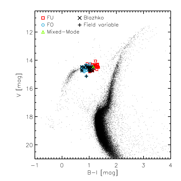
Figure 9: Optical (V,B–I) color-magnitude diagram of $\omega$ Cen. Light blue circles and red squares mark FO and F RRLs. The candidate RRd variable V142 is marked in green. The candidate FO field variable (V168) is marked with a black plus, while the black crosses display candidate Blazhko stars.

The current photometry allowed us to derive an accurate CMD covering not only the bright region typical of RGB and AGB stars (V$\sim$11-12 mag), but also $\sim$3 magnitudes fainter than the main sequence turn-off region. Fig. 9 shows the optical V, B–I CMD of $\omega$ Cen. The stars plotted in the above CMD have been selected using the photometric error ($\sigma_{V}\sim$0.03, $\sigma_{B-I}\sim$0.04 mag), the $\chi$ parameter (< 1.8), quantifying the deviation between the star profile and the adopted Point Spread Function (PSF), and the sharpness ($\bigl{|}sha\bigr{|}$ $<$ 0.7) quantifying the difference in broadness of the individual stars compared with the PSF. In passing we note that PSF photometry of individual images is mandatory to improve the precision of individual measurements of variable stars. The identification and fitting of faint sources located near the variable stars provides an optimal subtraction of light contamination from neighboring stars.

On top of the cluster photometry, Fig. 9 also shows the 170 out of the 195 RRLs for which we estimated both B-, V- and I-band mean magnitudes. The light blue, red and green symbols display RRc, RRab and the candidate RRd variable. The RRc are located, as expected, on the blue (hot) side of the instability strip, while the RRab are in the red (cool) region of the instability strip (Bono et al., 1997c). The crosses mark candidate Blazhko variables. The black plus sign identifies a candidate RRc field variable—V168—with a mean visual magnitude that is $\sim$0.6 mag fainter than cluster variables.

To further define the range in magnitude and colors covered by cluster RRLs, the left panel of Fig.10 shows a zoom across the instability strip. The blue and the red lines display the predicted hot (blue) edge for FO pulsators (FOBE) and the cool (red) edge for F pulsators (FRE). Note that the predicted edges are based on the analytical relations provided by Marconi et al. (2015) (see their Table 5). We assumed a metal content $\log{Z}$ = 0.0006 and an $\alpha$-enhanced chemical mixture ([$\alpha$/Fe]=0.4). This means an iron abundance of [Fe/H]=–1.81 These iron and $\alpha$-element abundances are consistent with the peak in the metallicity distribution of evolved stars in $\omega$ Cen based on recent spectrophotometric (Calamida et al., 2009) and spectroscopic (Johnson & Pilachowski, 2010) measurements. The agreement between theory and observations is remarkable if we take account for the theoretical and empirical uncertainties at the HB luminosity level. The former include a $\sim$50 K uncertainty on the temperature of the computed models, taking account for the adopted step in temperature (Di Criscienzo et al., 2004), plus uncertainties in color-temperature transformations ($\sigma_{B-I}\approx$0.05 mag). The empirical uncertainty on both the FRE and the FOBE is $\sigma_{B-I}\sim$0.05 mag. Note that the possible occurrence of differential reddening ($\Delta$E(B–V)=0.04 mag, (Moni Bidin et al., 2012)) mainly causes an increase in the photometric dispersion across the boundaries of the instability strip. The distribution of the RRLs inside the instability strip shows two interesting empirical features worth being discussed in more detail.

Magnitude distribution—To provide firm estimates of spread in visual magnitude of the $\omega$ Cen RRLs we performed an analytical fit of the observed distribution. The right panel of Fig. 10 shows the observed V magnitude distribution as a blue histogram. To overcome deceptive uncertainties in the criteria adopted to bin the data, we smoothed the distribution assigning to each RRL a Gaussian kernel (Di Cecco et al., 2010) with a $\sigma$ equal to the intrinsic error of the mean magnitude. The red curve was computed by summing the individual Gaussians over the entire dataset. The main peak appears well defined and located at $\sim$14.5 mag. To provide a more quantitative analysis, we fit the smoothed magnitude distribution with four Gaussian functions (purple curves). Note that the number of Gaussians is arbitrary: they were included only to minimize the residuals between analytical and observed distribution. The black solid curve shows the sum of the four Gaussians over the entire magnitude range. The data listed in Table 5 indicate that the two main peaks are located at V$\sim$14.47 and V$\sim$14.56 mag and include a significant fraction of the entire RRL sample, $\approx$51% and $\approx$25%, respectively. The fainter and the brighter peaks are located at V$\sim$14.71 and V$\sim$14.31 mag and roughly include $\approx$11% and $\approx$13% of the RRL entire sample. This suggests the metal-rich and the metal-poor tail produce only a minor fraction of RRLs. The above spread in optical magnitude indicates, for a canonical $M_{V}^{RR}$ vs [Fe/H] relation (Bono et al., 1997a), that $\omega$ Cen RRLs cover a range in iron abundance of the order of 1.5 dex (see also § 8).

Blazhko RR Lyrae—The data in the left panel of Fig. 10, indicate that a significant fraction (39%) of candidate Blazhko RRLs belongs to the fainter peak (V$\geq$14.6 mag). Preliminary evidence of clustering in magnitude and in color of Blazhko RRLs, has been found in M3 by Catelan (2004a), but a Kolmogorov-Smirnov test gave negative results. We have performed the same test on the B–Vand B–Icolor distributions of Blazhko RRLs versus RRab and RRc variables. We found that the probability the color distribution of Blazhko RRLs being equal to the color distribution of RRab and RRc is on average smaller than 1%. Moreover, we also confirm the preliminary empirical evidence based on the Bailey diagram (see § 3.5): they are mainly located between the FO and the F instability region. The above finding suggests that candidate Blazhko RRLs in $\omega$ Cen attain intermediate colors/temperatures.

Moreover, the difference in mean visual magnitude between the fainter (V$\geq$14.6 mag) and the brighter (V$<$14.6 mag) sample is also suggesting that the former ones are slightly more metal-rich. This working hypothesis is supported by metallicity estimates based on spectrophotometric indices (Rey et al., 2000) suggesting, for fainter and brighter Blazhko RRLs, mean metallicities of –1.4$\pm$0.3 and –1.8$\pm$0.1 dex (see, e.g., § 8). Metallicity estimates based on spectroscopic measurements (Sollima et al., 2006a) support the same finding, and indeed the mean iron abundances for fainter and brighter Blazhko RRLs are –1.2$\pm$0.1 and –1.7$\pm$0.2 dex, respectively. In passing, we also note that empirical evidence indicates that the Blazhko phenomenon occurs with higher frequency in more metal-poor environments (Kunder et al., 2013b). Homogeneous and accurate spectroscopic iron abundances are required to further investigate this interesting preliminary result.

5 Comparison with RR Lyrae in globulars and in dwarf galaxies

The large number of RRLs in $\omega$ Cen allows us to perform a detailed comparison with pulsation and evolutionary properties of RRLs in nearby stellar systems. To overcome thorny problems caused by small number statistics we selected, following Fiorentino et al. (2015), only GGCs hosting at least three dozen (35) RRLs. They are 16 out of the $\sim$100 GGCs hosting RRLs (Clement et al., 2001). To characterize the role played by the metallicity in shaping their pulsation properties they were divided, according to their metal content (Harris, 1996), into four different groups:

OoI—including 402 RRab, 6 RRd and 165 RRc with iron abundances ranging from [Fe/H]=–1.00 to –1.50;

OoInt—including 324 RRab, and 50 RRc with iron abundances ranging from [Fe/H]=–1.50 to –1.65;

OoII—including 111 RRab, 28 RRd and 111 RRc with iron abundances ranging from [Fe/H]=–1.65 to –2.40.

OoIII—including 60 RRab, 1 RRd and 41 RRc belonging to the two metal-rich globulars (Pritzl et al., 2001, 2002, 2003) NGC 6388 ([Fe/H]=–0.55) and NGC 6441 ([Fe/H]=–0.46). Note that we did not include the RRLs recently identified in Terzan 10 and in 2MASS-GC 02 by Alonso-García et al. (2015), since these two clusters still lack accurate spectroscopic measurements of the iron abundance.

The data for RRLs in GGCs were complemented with similar data for RRLs in nearby gas-poor stellar systems, namely dwarf spheroidal (dSph) and Ultra Faint Dwarf (UFD) galaxies. Note that we did not apply any selection criterion on the number of RRLs in building up this sample. We ended up with a sample of 1306 RRab, 50 RRd and 369 RRc with iron abundances ranging from [Fe/H]=–2.6 to [Fe/H]=–1.4 (Kirby et al., 2013; McConnachie, 2012; Fabrizio et al., 2015).

The double-mode variables—RRd—pulsate simultaneously in two different radial modes, typically F and FO. However, the latter is, with only a few exceptions (V44 in M3, Jurcsik et al., 2015), the main mode. However, they were not plotted in the Bailey diagram, since the separation of F and FO light curves does require very accurate and well sampled light curves (Coppola et al., 2015). They were also excluded from the period distribution, but included in the RRL population ratio, i.e., the ratio between the number of RRc and the total number of RRLs ($N_{c}/N_{tot}$). We plan to provide a more detailed analysis of RRd variables in a follow-up paper.

In this context it is worth mentioning that the RRLs that in the Clement catalog are classified as second overtones—RRe—were treated as RRc variables. Theoretical and empirical evidence indicates that the steady decrease in the pulsation period of RRc variables is mainly caused by a steady increase in metal content (Bono et al., 1997b). Note that the conclusions concerning the comparison between RRLs in $\omega$ Cen and in the other stellar systems are minimally affected by the inclusion of double-mode and possible candidate second overtone RRLs.

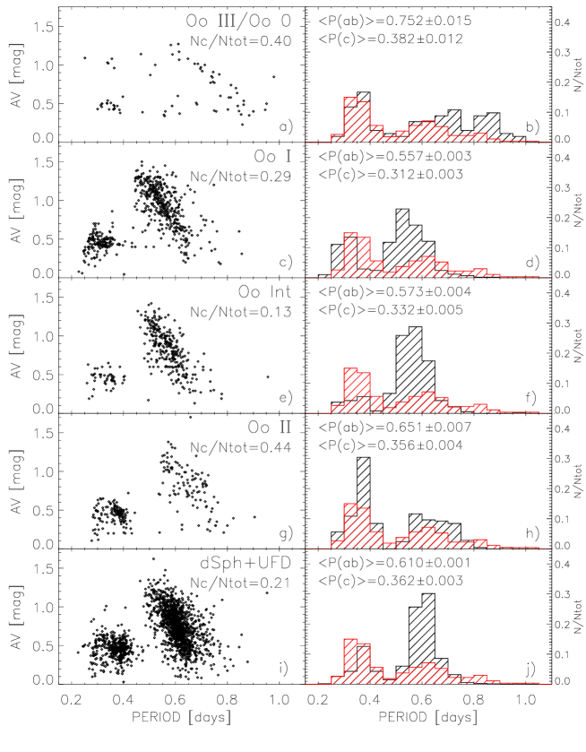
Figure 11: Panel a): Bailey diagram of the RRLs in the two OoIII/Oo0 metal-rich GGCs NGC 6388 and NGC 6441. Panel b): Comparison between the period distribution of RRLs plotted in Panel a) (black shaded area) and in $\omega$ Cen (red shaded area). The mean periods of RRab and RRc and the population ratio (number of RRc over the total number of RRLs) of the two GCs are also labeled. Panel c) and d): Same as a) and b), but for OoI GGCs with more than 35 RRLs. Panel e) and f): Same as a) and b), but for OoInt GGCs with more than 35 RRLs. Panel g) and h): Same as a) and b), but for OoII GGCs with more than 35 RRLs. Panel i) and j): Same as a) and b), but for dwarf spheroidals (dSph) and Ultra-Faint Dwarf (UFD) galaxies.

We estimated the diagnostics adopted to describe the Oosterhoff dichotomy: mean RRab and RRc periods and RRL population ratio for the stellar systems considered here, and their values are listed in Table 6 together with their uncertainties. We have already mentioned in Section 3.4 that $\omega$ Cen RRLs follow quite closely OoII clusters. However, data listed in this table together with the amplitudes and the period distributions plotted in Fig. 11 display several interesting trends worth being discussed.

i)—Linearity—The mean periods display a steady increase when moving from more metal-rich to more metal-poor stellar systems. The exception in this trend is given by the two metal-rich Bulge clusters (NGC 6388, NGC 6441). They are at least a half dex more metal-rich than OoI clusters, but their mean periods are from $\sim$25% (RRc) to $\sim$35% (RRab) longer. In passing we note that the above findings suggest that metal-rich globulars hosting RRLs belong to the Oosterhoff type 0 clusters instead of the OoIII group. This is the reason why their amplitudes and periods were plotted on top of Fig. 11 (see also the discussion in Section 9). On the other hand, the RRL population ratio shows a nonlinear trend, and indeed the OoInt clusters display a well defined minimum when compared with OoI, OoII and OoIII/Oo0 clusters. The decrease ranges from more than a factor of two with OoI to more than a factor of three with OoII and OoIII/Oo0 clusters. The RRLs in dwarf galaxies appear to attain values typical of stellar systems located between OoInt and OoII clusters. Note that the RRc mean period attains very similar values in dwarfs, in OoII clusters and in $\omega$ Cen, thus suggesting a limited sensitivity of this parameter in the more metal-poor regime.

ii)—Nature—The results mentioned in the above paragraph open the path to a long-standing question concerning the nature of $\omega$ Cen, i.e., whether it is a massive globular cluster or the former core of a dwarf galaxy. To further investigate this interesting issue we performed a more quantitative comparison between RRLs in $\omega$ Cen and in the aforementioned gas-poor stellar systems. The data in the left panels of Fig. 11 display two clear features: a) $\omega$ Cen and dwarf galaxies lack of High Amplitude Short Period (HASP) RRLs, i.e., F variables with P$\lesssim$0.48 days and $AV$ $>$ 0.75 mag (Stetson et al., 2014b). Empirical and theoretical evidence indicates that they become more and more popular in stellar systems more metal-rich than [Fe/H]$\approx$ –1.4/–1.5 (Fiorentino et al., 2015). Therefore, the paucity of HASPs in $\omega$ Cen is consistent with previous metallicity estimates available in the literature (Calamida et al., 2009; Johnson & Pilachowski, 2010), and with the current metallicity estimates (see Section 8). We estimated the marginals of the Bailey diagrams plotted in the left panels of the above figure plus $\omega$ Cen and the $\chi^{2}$ analysis indicates that the latter agrees with OoII clusters at the 94% confidence level. The agreement with the other Bailey diagrams is either significantly smaller (39%, OoIII/Oo0; 42%, dwarfs) or vanishing (OoI, OoInt).

On the other hand, the comparison of the period distributions plotted in the right panels of Fig. 11 clearly display that $\omega$ Cen is similar to an OoII cluster. Moreover, RRLs in $\omega$ Cen and in dwarf galaxies also display similar metallicity distributions. However, the coverage of the RRL instability strip in the former system appears to be more skewed toward the FO region than toward the F region as in the latter ones. The above difference is further supported by the stark difference in the population ratio and in the peaks of RRab and RRc period distributions. We also performed the $\chi^{2}$ analysis of the period distributions plotted in the right panels of Fig. 11 and we found that RRLs in $\omega$ Cen agree with OoII clusters at the 80% confidence level. The agreement with the other samples is either at a few percent level or vanishing (dwarfs). Therefore, the working hypothesis that $\omega$ Cen is the core remnant of a spoiled dwarf galaxy (Zinnecker et al., 1988; Freeman, 1993; Bekki & Freeman, 2003) does not find solid confirmation by the above findings. This result is somehow supported by the lack of firm signatures of tidal tails recently found by (Fernández-Trincado et al., 2015a, b) using wide field optical photometry covering more than 50 $deg^{2}$ around the cluster center.

iii)—Nurture—$\omega$ Cen RRLs display a well defined long-period tail (P$>$0.8 days) that is barely present in the RRL samples of the other systems. The exception is, once again, given by the two metal-rich globulars hosting RRLs, namely NGC 6388 and NGC 6441. A detailed analysis of the HB luminosity function is beyond the aim of the current investigation, however, we note that $\omega$ Cen and the two Bulge clusters share an indisputable common feature, i.e., the presence in the HB luminosity function of a well extended blue tail. This suggests us that its presence is more nurture than nature. The environment, and in particular, the high central density, might play a crucial role in the appearance of the blue tail, and in turn in the appearance of long-period RRLs (Castellani et al., 2006). Indeed, it has been suggested (Castellani et al., 2007; Latour et al., 2014) that either binarity or stellar encounters might explain the presence of extended blue tails, and in turn, an increased fraction of blue HB stars evolving from the blue to the red region of the CMD. However, it is worth noting that the above evidence is far from taking account of the current empirical evidence, and indeed the metal-intermediate ([Fe/H]=–1.14 Carretta et al., 2009) globular NGC 2808 hosts 11 RRab variables, but they have periods shorter than 0.62 days (Kunder et al., 2013a). It has also been suggested that a possible spread in helium abundance might also take account for the HB morphology in $\omega$ Cen Tailo et al. (2016), and in turn of the period distribution of RRLs. However, the increase in helium content is degenerate with possible evolutionary effects (Marconi et al., 2011) and we still lack firm conclusions. The reader interested in a recent detailed discussion concerning the Oosterhoff dichotomy and the HB morphology is referred to Jang & Lee (2015).

Finally, we would like to underline that the above results strongly support the idea that only a limited number of GCs are good laboratories to understand the origin of the Oosterhoff dichotomy. The main limitations being statistics and environmental effects. This evidence further suggests that the metallicity is the main culprit in shaping the above empirical evidence, while the HB luminosity function appears to be the next more plausible candidate. In passing, we also mention that a steady increase in helium content has also been suggested to take account of the extended blue tail in Galactic globulars (NGC 2808, D’Antona et al., 2005). The increase in helium content causes a steady increase in the pulsation period of both RRc and RRab variables (Marconi et al., 2011). Firm constraints require detailed sets of synthetic HB models accounting for both the HB morphology and the period distribution (Salaris et al., 2013; Sollima et al., 2014; Savino et al., 2015). We plan to investigate this issue in a forthcoming paper, since $\omega$ Cen is the perfect laboratory to constrain the transition from RRLs to TIICs.

6 RR Lyrae diagnostics

6.1 Period-Luminosity relations

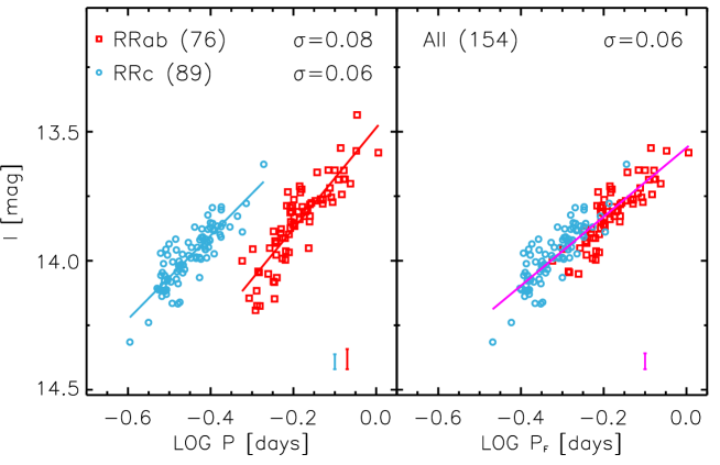
Figure 12: Left: Empirical I-band Period-Luminosity (PL) relation for $\omega$ Cen RRLs. Light blue and red squares mark RRc and RRab variables. The light blue and the red lines display the linear fits, while the vertical bars show the standard deviations, $\sigma$, of the fits. The number of variables adopted in the fits are also labeled. Right: Same as the left, but for the global (RRc$+$RRab) RRL sample. The periods of RRc variables were fundamentalized using $\log{P_{F}}=\log{P_{FO}}+0.127$.

On the basis of both periods and mean magnitudes measured in Section 3.3 and in Section 3.2, we estimated the empirical I-band PL relations of $\omega$ Cen RRLs. Following Braga et al. (2015) and Marconi et al. (2015) we evaluated the PL relations for RRc, RRab and for the global (All) sample. In the global sample the RRc were “fundamentalized”, i.e., we adopted $\log{P_{F}}=\log{P_{FO}}+0.127$ (Iben & Huchra, 1971; Rood, 1973; Cox et al., 1983; Di Criscienzo et al., 2004; Coppola et al., 2015). The coefficients, their errors and the standard deviations of the empirical PL relations are listed in Table 7. The RRLs adopted to estimate the PL relations are plotted in Fig. 12.

Note that we derived the PL relations only in the I-band because theoretical (Bono et al., 2001; Catelan et al., 2004; Marconi et al., 2015) and empirical (Benkő et al., 2011; Braga et al., 2015) evidence indicates that RRLs do not obey to a well defined PL relation in the U, B and V band. Moreover, in the R-band, the dispersion is large ($\sim$0.15 mag) and the slope is quite shallow ($\sim$-0.5 mag).

The standard deviations plotted in the bottom right corner of Fig. 12 and the modest intrinsic error on the mean I-band magnitude discussed in § 3.3 clearly indicate that the dispersion of the empirical I-band PL relation is mainly caused by the spread in metal abundance of $\omega$ Cen RRLs (see Section 8). Indeed, pulsation and evolutionary predictions (Bono et al., 2003a; Catelan et al., 2004; Marconi et al., 2015) indicate that the zero-points of the I-band PL relations do depend on metal abundance. We will take advantage of this dependence to estimate individual RRL metal abundances (see § 8).

6.2 Period-Wesenheit relations

The Period-Wesenheit (PW) relations, when compared with the PL relations, have the key advantage to be reddening-free by construction (Van den Bergh, 1975; Madore, 1982). This difference relies on the assumption that the adopted reddening law is universal (Bono et al., 2010). The pseudo Wesenheit magnitude is defined as

$$W(X,Y-Z)=X+\dfrac{A_{X}}{A_{Y}-A_{Z}}(Y-Z)$$ (1)

where X, Y and Z are the individual magnitudes and $A_{X}$, $A_{Y}$ and $A_{Z}$ are the selective absorption coefficients provided by the reddening law (Cardelli et al., 1989; Fitzpatrick & Massa, 2007). We have adopted the popular reddening law of Cardelli et al. (1989) with $R_{V}=3.06$ and $A_{B}$/$A_{V(Johnson)}$=1.348, $A_{V}$/$A_{V(Johnson)}$=1.016 $A_{I}$/$A_{V(Johnson)}$=0.590). Note that, to match the current optical photometric system (Landolt, 1983, 1992), the original $R_{V}$ value ($R_{V}=3.1$) and the selective absorption ratios provided by Cardelli et al. (1989) were modified accordingly.

Fig. 13 shows the dual—and the triple—band empirical PW relations for $\omega$ Cen RRLs. The coefficients, their errors and the standard deviations of the PW relations are listed in Table 8. The slopes of the PW relations listed in this Table agree, withing the errors, remarkably well with the slope predicted by nonlinear, convective hydrodynamical models of RRLs (Marconi et al., 2015, see their Tables 7 and 8). Indeed, the predicted slopes for the metal independent PW(V,B–V) relations range from –2.8, (FO), to –2.7 (F) and to –2.5 (global), while for the metal-dependent PW(V,B–I) relations they range from –3.1 (FO), to –2.6 (F) and to –2.5 (global). The comparison in the latter case is very plausible, since the coefficient of the meatllicity term for the PW(V,B–I) relations is smaller than 0.1 dex. The predicted slope for FO variables is slightly larger, but this might be due to the limited sample of adopted FO models.

The current empirical slopes for the optical PW relations agree quite well with similar estimates recently provided by Coppola et al. (2015) for more than 90 RRLs of the Carina dSph. They found slopes of –2.7 [global, PW(V,B–V)] and –2.6 [global, PW(V,B–I)], respectively. The outcome is the same if we take account for the thorough analysis performed by Martínez-Vázquez et al. (2015) for the 290 RRLs (clean sample) of Sculptor dSph, namely –2.5 [global, PW(V,B–I)] and –2.7 [global, PW(V,B–I)]. The reader interested in a detailed discussion concerning the physical arguments supporting the universality of the above slope is referred to the recent investigation by Lub (2016).

The data in Fig. 13 display that the standard deviation of the different PW relations steadily decrease if either the effective wavelength of the adopted magnitudes increases (see panels c), d) e) and f)) and/or the difference in effective wavelength of the adopted color increases (see panels d) and h). Finally, we note that the standard deviations of the PW(V,B–V) relations are systematically larger than the other PW relations. The difference is mainly caused by the fact that this PW relation has the largest color coefficient (3.06), and in turn, the largest propagation of the intrinsic errors on mean colors.

7 Distance determination

The $\omega$ Cen RRLs cover a broad range in metal abundance. This means that accurate distance determinations based on diagnostics affected by the metal content do require accurate estimates of individual iron abundances (Del Principe et al., 2006; Bono et al., 2008a). The observational scenario concerning iron abundances of $\omega$ Cen RRLs is far from being ideal. Estimates of the iron abundance for 131 RRLs in $\omega$ Cen were provided by Rey et al. (2000, hereinafter R00) using the hk photometric index introduced by Baird (1996). More recently, Sollima et al. (2006a, hereinafter S06) estimated iron abundances for 74 RRLs in $\omega$ Cen using moderately high-resolution spectra collected with FLAMES at VLT. These iron abundances are listed in columns 1 and 2 of Table 10. The former sample is in the globular cluster metallicity scale provided by Zinn & West (1984, hereinafter ZW84).

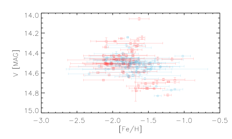
Figure 14: V vs [Fe/H] distribution of $\omega$ Cen RRLs. We adopted iron abundances available in the literature (Rey et al., 2000; Sollima et al., 2006a) rescaled into the Carretta et al. (2009) metallicity scale. The vertical error bars display errors in the mean visual magnitude, while the horizontal ones either the intrinsic error (single measurement) or the standard deviation (two measurements). See text for more details.

They were transformed into the homogeneous and accurate metallicity scale provided by Carretta et al. (2009) using their linear transformation (see their § 5). The iron abundances provided by S06 were estimated following the same approach adopted by Gratton et al. (2003); Carretta et al. (2009). They were transformed into the Carretta’s metallicity scale once accounting for the difference in the solar iron abundance ($log{\epsilon_{Fe_{\odot}}}$=7.52 vs 7.54). Fortunately enough, the two samples have 52 objects in common. We estimated the difference between R00 and S06 and we found $\Delta$[Fe/H]=0.18$\pm$0.03 ($\sigma$=0.20). We rescaled the R00 to the S06 iron abundances and computed the mean for the objects in common (see column 4 in Table 10). Figure 14 shows the entire sample of $\omega$ Cen RRLs (153) for which a metallicity estimate is available in the [Fe/H]–V plane. A glance at the data in this figure shows that the current uncertainties on individual iron abundances are too large to provide precise distance determinations. Indeed, the uncertainties on iron abundances range from less than 0.1 dex to more than 0.5 dex.

The above empirical scenario is further complicated by the evidence that $\omega$ Cen might also be affected by differential reddening (Dickens & Caldwell, 1988; Calamida et al., 2005; Majewski et al., 2012) at a level of $\Delta$E(B-V)=0.03-0.04 mag (Moni Bidin et al., 2012).

To overcome the above thorny problems we decided to take advantage of recent findings concerning the sensitivity of optical and NIR diagnostics on metallicity and reddening to estimate RRL individual distances. Pulsation predictions indicate that the spread in magnitude of optical and NIR PW relations is smaller when compared with the spread typical of optical and NIR PL relations. This finding applies to both RRLs and classical Cepheids. The decrease in magnitude dispersion is mainly caused by the fact that the PW relations mimic a Period-Luminosity-Color (PLC) relation. Thus taking account for the individual position of variable stars inside the instability strip (Bono & Marconi, 1999; Udalski et al., 1999; Soszyński et al., 2009; Marconi et al., 2015). Moreover and even more importantly, theory and observations indicate that the PW(V,B–V  and V,B–I) relations display a minimal dependence on metallicity. Indeed, their metallicity coefficients are at least a factor of two smaller when compared with similar PW relations (Marconi et al., 2015; Coppola et al., 2015; Martínez-Vázquez et al., 2015).

For the reasons already mentioned in § 6.2 (smaller standard deviation, smaller color coefficient) and above, we adopted the PW(V,B–I) relations to estimate the distance to $\omega$ Cen. To quantify possible uncertainties either on the zero-point or on the slope, we estimated the distance using the observed slope and the predicted zero-point (semi-empirical) and predicted PW relation (theoretical, see Table 8 by Marconi et al. (2015)).

Using the metal-independent semi-empirical calibrations obtained using the observed slopes and the predicted zero-points (Marconi et al., 2015) we found that the distance modulus to $\omega$ Cen (see also Table 9) ranges from 13.74$\pm$0.08 (statistical) $\pm$0.01 (systematic) mag (FO) to 13.69$\pm$0.08$\pm$0.01 mag (F) and to 13.71$\pm$0.08$\pm$0.01 mag (global). The statistical error is the dispersion of the distribution of the distance moduli of individual RRLs. The systematic error is the difference between the theoretical and the semi-empirical calibration of the PW(V,B–I) relations. The current estimates agree within 1$\sigma$ and the mean weighted distance modulus is 13.71$\pm$0.08$\pm$0.01 mag. We estimated the distance modulus using also theoretical calibration and we found 13.74$\pm$0.08$\pm$0.01 mag (FO), 13.70$\pm$0.08$\pm$0.01 mag (F) and 13.71$\pm$0.08$\pm$0.01 mag (global). The new distance moduli agree with those based on the semi-empirical calibration and the mean weighted distance modulus is 13.71$\pm$0.08$\pm$0.01 mag.

The distance moduli that we derived, agree quite well with similar estimates based on the K-band PL relation of RRLs provided by Longmore et al. (1990) (13.61 mag), Sollima et al. (2006b) (13.72 mag), (Bono et al., 2008b) (13.75$\pm$0.11 mag), by Del Principe et al. (2006) (13.77$\pm$0.07 mag) and Navarrete et al. (2016) (13.70$\pm$0.03 mag).

A similar remarkable agreement is also found when comparing the current distance moduli with those based on the TRGB provided by Bellazzini et al. (2004) (13.70$\pm$0.11 mag) and by Bono et al. (2008b) (13.65$\pm$0.09 mag). The current estimates also agree within 1$\sigma$ with both distance moduli provided by Kaluzny et al. (2007) using cluster eclipsing binaries—namely $\mu$=13.49$\pm$0.14 and $\mu$=13.51$\pm$0.12 mag—and with the kinematic distance to $\omega$ Cen provided by van de Ven et al. (2006, $\mu$=13.75$\pm$0.13 mag). The kinematic distance method applied to GCs is a very promising and independent primary distance indicator based on the ratio between the dispersions in proper motion and in radial velocity of cluster stars. The key advantage of this diagnostic is that its accuracy is only limited by the precision of the measurements and by the sample size (King & Anderson, 2002). The above difference seems to suggest the possible unrecognized systematic errors. The reader interested in a more detailed discussion concerning the different diagnostics adopted to estimate cluster distances is referred to Bono et al. (2008b).

Note that we are not providing independent distance estimates to $\omega$ Cen using the zero-point based on the five field RRLs for which are available trigonometric parallaxes (Benedict et al., 2011). The reason is twofold: a) preliminary empirical evidence based on optical, NIR and MIR measurements indicates that their individual distances might require a mild revision (Neeley et al. 2016, in preparation); b) we plan to address on a more quantitative basis the accuracy of $\omega$ Cen distance, using optical, NIR and MIR mean magnitudes of RRLs (Braga et al. 2016, in preparation).

8 Metallicity of RR Lyrae stars

Dating back to the spectroscopic surveys of giant stars by Norris et al. (1996) and Suntzeff & Kraft (1996), we have a clear and quantitative evidence that $\omega$ Cen hosts stellar populations characterized by a broad spread in iron abundances. More recently, Fraix-Burnet & Davoust (2015), by analyzing the abundances provided by Johnson & Pilachowski (2010), confirmed the presence of three main populations as originally suggested by Norris & Da Costa (1995), Smith et al. (2000), Pancino et al. (2002) and Vanture et al. (2002). The general accepted scenario is that of a globular with a dominant metal-poor primordial population (–2.0 $<$ [Fe/H] $<$ –1.6) plus a metal-intermediate (–1.6 $<$ [Fe/H] $<$ –1.3) and a relatively metal-rich (–1.3 $<$ [Fe/H] $<$ –0.5) population. The reader is also referred to Calamida et al. (2009), for a detailed discussion concerning the spread in iron abundance based on the Stroemgren metallicity index for a sample of $\sim$4000 stars.

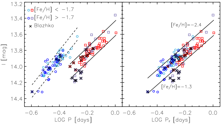
Figure 15: Left: Empirical I-band PL relation for $\omega$ Cen RRLs. Light blue circles and red squares mark variables more metal-poor than [Fe/H] = –1.7, while blue circles and violet squares mark variables more metal rich than [Fe/H] = –1.7. Candidate Blazhko stars are marked with a black cross. The black lines display predicted (Marconi et al., 2015) I-band PLZ relation for F (solid) and FO pulsators at fixed metal abundance [Fe/H] = –2.4 (brighter) and [Fe/H] = –1.3 (fainter). Right: Same as the left, but for the global (RRc$+$RRab) RRL sample. The periods of RRc variables were fundamentalized using $\log{P_{RRab}}=\log{P_{RRc}}+0.127$.

To further constrain the plausibility of the theoretical framework adopted to estimate the distances and to validate the current metallicity scale we compared theory and observations in the $\log P$–$I$ plane. Figure 15 shows predicted I-band empirical PL relation at different iron abundances (see labeled values) together with $\omega$ Cen RRLs. Note that the objects for which are available iron abundance estimates (R00, S06) were plotted using a color code: more metal-poor ([Fe/H] $<$ –1.7) RRLs are marked with light blue (RRc) and red (RRab) colors, while more metal-rich ([Fe/H] $>$ –1.7) with blue (RRc) and violet (RRab) colors. The adopted iron values are based on the R00+S06 homogenized sample, listed in column 4 of Table 10. The data in this figure display two interesting features worth being discussed.

i) Predicted PL relation at different iron abundances and observed range in iron abundance of RRLs agree quite well, and indeed, the former ones bracket the bulk ($\sim$80%) of the RRL sample. Moreover, there is a mild evidence of a ranking in metallicity, indeed more metal-rich RRLs appear—on average—fainter than metal-poor ones. This evidence applies to both RRab ($\Delta I_{poor-rich}\sim 0.15$ mag) and to RRc ($\Delta I_{poor-rich}\sim 0.09$ mag) variables.

ii) Blazhko variables are mostly located between RRc and RRab variables. Moreover, they also appear to be more associated with more metal-poor (14) than with more metal-rich (11) RRLs, the ratio being 1.27. The trend is similar to non-Blazhko RRLs, for which the more metal-poor sample (78) is even larger than the more metal-rich one (50, the ratio is 1.56). Note that we did not take account of RRLs for which iron abundance is not available (35 non-Blazhko and three Blazhko RRLs). It is clear that $\omega$ Cen is the right laboratory to delineate the topology of the instability strip, due to sample size and the broad spread in iron abundance. Its use is currently hampered by the lack of accurate and precise elemental abundances for the entire RRL sample.

On the basis of the above empirical evidence, we decided to take advantage of the accuracy of the distance modulus to $\omega$ Cen and of the sensitivity of the I-band PL relation to provide a new estimate of the iron abundance of individual RRLs. A similar approach was adopted by Martínez-Vázquez et al. (2015) and by Coppola et al. (2015) to estimate the metallicity distribution of RRLs in Sculptor and in Carina, respectively. The absolute I-band magnitudes ($M_{I}$) of RRLs were estimated using the true distance modulus ($\mu$=13.70$\pm$0.02 mag) based on theoretical PW relations (see § 7). In particular, $M_{I}=I-A_{I}-\mu$, where $\mu$ is the true distance modulus and $A_{I}$ the selective absorption in the I-band. We also adopted, according to Thompson et al. (2001); Lub (2002), a cluster reddening of $E(\hbox{\it B--V\/})$ = 0.11 mag. We took also account of the spread in $E(\hbox{\it B--V\/})$ measured by Moni Bidin et al. (2012). According to the reddening law provided by Cardelli et al. (1989), we adopted a ratio $A_{I}$/$A_{V}$ = 0.590. Note that the current value accounts for the current photometric system (see for more details Section 6.2).

Finally, theoretical I-band PLZ relation for F and FO pulsators were inverted to estimate the metallicities of $\omega$ Cen RRLs:

$$\mathrm{[Fe/H]}=\dfrac{M_{I}-b\log{P}-a}{c}$$ (2)

where $a$, $b$ and $c$ are the zero-point, the slope and the metallicity coefficient of the predicted PLZ relations in the form $M_{I}=a+b\log{P}+c\mathrm{[Fe/H]}$. The values of the coefficients $a$, $b$ and $c$ are listed in Table 6 of Marconi et al. (2015). Note that we adopted this relation, because theory and observations indicate that PL relations are less prone to systematic uncertainties introduced by a spread in stellar mass and/or in stellar luminosity due to evolutionary effects (Bono et al., 2001; Bono, 2003). To estimate the iron abundance, we only took into account RRLs with photometric error in the I band smaller than 0.1 mag. To provide a homogeneous metallicity scale for $\omega$ Cen the above estimates (solar iron abundance in number $log{\epsilon_{Fe_{\odot}}}$=7.50, Pietrinferni et al., 2006; Marconi et al., 2015) were rescaled to the homogeneous cluster metallicity scale provided by Gratton et al. (2003); Carretta et al. (2009) ($log{\epsilon_{Fe_{\odot}}}$=7.54).

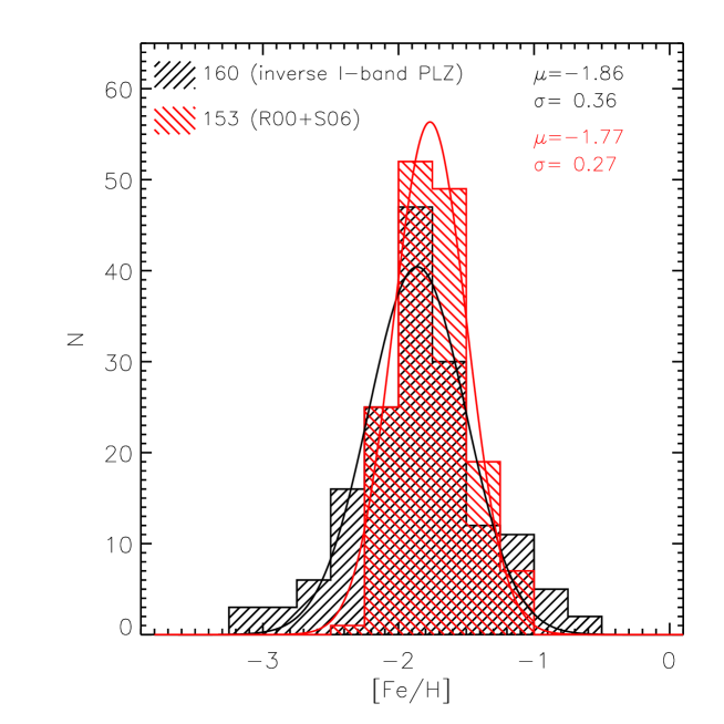
Figure 16: Iron distribution of $\omega$ Cen RRLs. The black shaded area shows iron estimates based on the inversion of theoretical I-band PLZ relations for RRab and RRc variables. The red shaded area shows iron distribution based on measurements available in the literature and based on both spectroscopic (Sollima et al., 2006a) and photometric (Rey et al., 2000) estimates. The current and the literature iron abundances are in the homogeneous cluster metallicity scale provided by Carretta et al. (2009). The red and the black curves display the Gaussian fits of the observed distributions. The means and the $\sigma$s of the two Gaussians are also labelled.

The metallicity distribution based on 160 RRLs is plotted in Fig. 16 as a black shaded area together with the metallicity distribution based on iron abundances provided by R00 and by S06 (red shaded area). We fit the two iron distributions with a Gaussian and we found that current distribution is slightly more metal-poor, indeed the difference in the peaks is $\Delta$[Fe/H]=0.09. The $\sigma$ of the current distribution is larger—0.36 vs 0.27—than the literature one. The difference is mainly caused by the fact that the iron distribution based on S06 and R00 abundances displays a sharp cut-off at [Fe/H]$\sim$–2.3, while the current one attains iron abundances that are 0.5 dex more metal-poor. We double checked the objects located in the metal-poor tail. Nine out of twelve are RRc stars and we found that they mainly belong to the brighter group. There is also marginal evidence for a slightly more extended metal-rich tail, but the difference is caused by a few objects.

In passing, we note that the metal-poor tail is only marginally supported by both spectroscopic and photometric investigations based on cluster red giant stars. Indeed, Calamida et al. (2009) using Stroemgren photometry for $\sim$4000 red giants, found that the metallicity distribution can be fit with seven Gaussians. Their peaks range from [Fe/H]$\sim$–1.7 to [Fe/H]$\sim$+0.2. A similar result was also obtained by Johnson & Pilachowski (2010) using high-resolution spectra of 855 red giants, suggesting iron abundances ranging from [Fe/H] $\sim$ –2.3 to [Fe/H] $\sim$ –0.3 (see also Fraix-Burnet & Davoust, 2015).

As a consequence of the reasonable agreement in the iron distributions, we applied to the current iron distribution the difference in the main peaks and provided a homogeneous metallicity scale. For the objects in common with R00$+$S06 we computed a mean weighted iron abundance and the final values are listed in column 6 of Table 10.

It is worth mentioning that the current approach to estimate RRL iron abundances depends on the adopted distance modulus. A modest increase of 0.05 mag in the true distance modulus implies a systematic shift of $\sim$0.30 dex in the peak of the metallicity distribution. However, the current approach is aimed at evaluating the relative and not the absolute difference in iron abundance. This means that we are mainly interested in estimating either the spread (standard deviation) in iron abundance or the possible occurrence of multiple peaks in the metallicity distribution (Martínez-Vázquez et al., 2015).

9 Summary and final remarks

We present new accurate and homogeneous optical, multi-band—UBVRI—photometry of the Galactic globular $\omega$ Cen. We collected 8202 CCD images that cover a time interval of 24 years and a sky area of 84$\times$48 arcmin across the cluster center. The bulk of these images were collected with the Danish telescope at ESO La Silla as time-series data in three main long runs (more than 4,500 images). The others were collected with several telescopes ranging from the 0.9m at CTIO to the VLT at ESO Cerro Paranal. The final photometric catalog includes more than 180,000 (Danish) and 665,000 (others) stars with at least one measurement in two different photometric bands. The above datasets were complemented with optical time series photometry for RRLs available in the literature. The global photometric catalog allowed us to accomplish the following scientific goals.

Homogeneity—We provide new, homogeneous pulsation parameters for 187 candidate $\omega$ Cen RRLs. All in all the photometry we collected (proprietary$+$literature) covers a time interval of 36 years and the light curves of RRLs have a number of phase points per band that ranges from $\sim$10-40 (U), to$\sim$ 20-770 (B), to $\sim$20-2830 (V), to $\sim$10-280 (R) and to $\sim$10-445 (I). These numbers sum up to more than 300,000 multi-band phase points for RRLs, indicating that this is the largest optical photometric survey ever performed for cluster RRLs (Jurcsik et al., 2012, 2015). The above data allowed us to provide new and accurate estimates of their pulsation parameters (mean magnitudes, luminosity variation amplitudes, epoch of maximum and epoch of mean magnitude).

Period distribution—The key advantage in dealing with $\omega$ Cen is that its RRL sample is the 3^rd largest after M3 (237 RRLs) and M62 (217) among the globulars hosting RRLs. On the basis of the current analysis we ended up with a sample 187 candidate cluster RRLs. Among them 101 pulsate in the first overtone (RRc), 85 in the fundamental (RRab) mode and a single object is a candidate mixed-mode variable (RRd). We estimate the mean periods for RRab and RRc variables and we found that they are $<P_{ab}>=0.668$ days, $<P_{c}>=0.359$ days. The above mean periods and the population ratio, i.e., the ratio between the number of RRc and the total number of RRLs ($N_{c}/(N_{ab}+N_{d}+N_{c})$) support previous findings suggesting that $\omega$ Cen is a Oosterhoff II cluster.

Bailey Diagram—The luminosity variation amplitude vs period plane indicates a clear lack of HASP RRLs, i.e., RRab variables with P$\lesssim$0.48 days and $AV$ $>$ 0.75 mag (Fiorentino et al., 2015). These objects become more popular in stellar systems more metal-rich than [Fe/H] $\approx$ –1.4, thus suggesting that RRL in $\omega$ Cen barely approach this metallicity range. The RRab variables that, from our investigation, appear to be more metal-rich than –1.4, have periods ranging from 0.49 to 0.72 days.

Moreover, we also found evidence that RRc can be split into two different groups: a) short-period—with periods ranging from $\sim$0.30 to $\sim$0.36 days and visual amplitudes ranging from a few hundreths of a magnitude to a few tenths; b) long-period—with periods ranging from $\sim$0.36 to $\sim$0.45 days and amplitudes clustering around $AV\sim$0.5 mag. Theoretical and empirical arguments further support a well defined spread in iron abundance.

Amplitude ratios—The well known spread in iron abundance of $\omega$ Cen stars makes its RRL sample a fundamental test-bench to characterize the possible dependence of amplitude ratios on metal content. We performed a detailed test and we found that both RRab and RRc attain similar ratios: $AB/AV$ = 1.26$\pm$0.01; $AR/AV$ = 0.78$\pm$0.01; $AI/AV$ = 0.63$\pm$0.01. Moreover, they do not display any clear trend with iron abundance.

Visual magnitude distribution—We performed a detailed analysis of the visual magnitude distribution of RRLs and we found that they can be fit with four Gaussians. The two main peaks included a significant fraction of RRL ($\sim$76%) and attain similar magnitudes (V$\sim$14.47, 14.56 mag). The fainter (V$\sim$14.71 mag) and the brighter (V$\sim$14.31 mag) peak include a minor fraction (11%, 13%) of the RRL sample. The above finding is suggestive of a spread in iron abundance of the order of 1.5 dex and paves the way for new solid estimates on the absolute age of the different stellar populations in $\omega$ Cen.

Blazhko RR Lyrae—Empirical evidence based on the location of candidate Blazhko RRLs in the Bailey diagram and in the color-magnitude diagram clearly indicate that they are located between RRc and RRab variables. Indeed, we found that a significant fraction (79%) of them (22 out of 28) have periods shorter than 0.6 days. Moreover, their location inside the instability strip indicates that a significant fraction (39%) of them belongs to the fainter peak (V$\geq$14.6 mag), thus suggesting that this sub-sample is more associated with the more metal-rich stellar component.

Oosterhoff dilemma—Dating back to the seminal investigation by Oosterhoff (1939) in which he recognized that cluster RRLs can be split, according, to their mean periods, into two different groups, the astronomical community undertook a paramount observational effort in order to constrain the physical mechanism(s) driving the empirical evidence. We performed a detailed comparison between the period distribution and the Bailey diagram of $\omega$ Cen RRLs with globulars hosting a sizable sample (>35) of RRLs and with RRLs in nearby dSphs and UFDs. We found, as expected, that the mean F and FO periods display a steady decrease when moving from the more metal-rich (Oosterhoff I) to the more metal-poor (Oosterhoff II) clusters. In this context dSphs and UFDs attain values that are intermediate between the OoInt and the OoII clusters, while $\omega$ Cen appears as the upper envelope of the distribution. On the other hand, the population ratio—$N_{c}/(N_{ab}+N_{d}+N_{c})$—has a nonlinear trend, since it attains a well defined minimum for OoInt clusters. In spite of the possible differences, the iron abundance appears to be the key parameter in driving the transition from short mean periods to long mean periods stellar systems. The above results do not support the working hypothesis that $\omega$ Cen is the core remnant of dwarf galaxy (Bekki & Freeman, 2003). Moreover, there is mounting empirical evidence that cluster RRLs might not be the appropriate sample to address the Oosterhoff dichotomy, since they might be either biased by statistics or affected by environmental effects.

$\omega$ Cen disguised as a dwarf galaxy—The number of globulars hosting long-period (0.82–0.85$\lesssim$P$\lesssim$1 days) RRLs is quite limited. Three honorable exceptions are $\omega$ Cen and the two metal-rich Bulge globulars hosting RRLs, namely NGC 6388 and NGC 6441. The mean periods of the metal-rich clusters appear as an extreme case of OoI clusters. This is the reason why we suggest they should be classified as Oosterhoff type 0 instead of Oosterhoff type III. We note that the main common feature among these clusters is that the HB luminosity function shows a well developed blue tail. This indicates that the appearance of long-period RRLs is more nurture that nature. The environment, and in particular, the high central stellar density, might play a crucial role in the presence of a blue tail, and in turn of long-period RRLs. However, the observational scenario appears much more complex, since the RRLs in the metal-intermediate cluster NGC 2808 hosts 11 RRab variables, but they have periods shorter than 0.62 days (Kunder et al., 2013a).

Distance determination—We take advantage of optical PW relations that are reddening independent by construction and minimally dependent on iron abundance to provide new estimates of the distance to $\omega$ Cen. We adopted both a semi-empirical and a theoretical calibration and we found a true distance modulus of 13.71$\pm$0.08$\pm$0.01 mag. They agree quite well with similar estimates available in the literature. In particular, we found that the agreement is within 1$\sigma$ with the geometrical distances based on eclipsing binaries (13.49$\pm$0.14 / 13.51$\pm$0.12, Kaluzny et al., 2007).

Metallicity distribution—We inverted the I-band PLZ relation for F and FO pulsators to provide individual metallicity estimates for 160 cluster RRLs. We found that the metallicity distribution agrees quite well with the metallicity distribution of RRLs based on spectroscopic measurements (74, S06) and on photometric indicators (131, R00). We also found evidence of a metal-poor tail that is not present in previous spectroscopic investigations of $\omega$ Cen RRLs.

The current long-term photometric surveys are providing new and homogeneous measurements concerning field and cluster stars. The current status is going to experience a quantum jump as soon as the ongoing (Gaia) and near future ground-based experiments will release their data. The project we started more than 15 years ago on $\omega$ Cen, may be defined as a local survey. The number of optical images adopted to individuate main sequence and evolved variable stars have been discussed in detail on Section 2. In dealing with the Danish dataset we analyzed 4539 images and we performed $\approx 2.5\times 10^{8}$ measurements, which means roughly 55,000 stars per image. In dealing with all the other optical datasets we analyzed 3663 images and performed $\approx 1.1\times 10^{8}$ measurements, which means roughly 27,000 stars per image. A similar number of measurements have been also performed in dealing with NIR images. The above numbers indicate once accounting for the preliminary steps in approaching the final photometric catalog, that we are dealing with an experiment that included more than one giga measurements. The results concerning variable and static stars will be addressed in a series of future papers in which we plan to use homogeneous multi-band optical, NIR and MIR photometry.

Appendix A Notes on individual RR Lyrae stars

V4, V25, V44, V88, V90, V91, V271, V272, V273, V276, NV340, NV341, NV349, NV350, NV352— We estimate the pulsation parameters neglecting either the danish95 and/or the danish98 and/or the danish99 datasets, since they are noisy.

V5, V9, V11, V56, V67, V69, V74, V106, V112, V115, V120, V130, V140, V141— We confirm the Blazhko modulations suggested by Kaluzny et al. (2004) and Weldrake et al. (2007) and provide preliminary estimates of B- and/or V-band Blazhko amplitudes (see Table 3).

V10, V24, V32, V47, V58, V64, V70, V71, V77, V81, V82, V87, V89, V95, V123, V124, V126, V131, V136, V145, V147, V153, V155, V156, V157, V158, V166, V270, V275, V289, NV340, NV346, NV347, NV353, NV354— There is mild evidence of a period change.

V11, V94— There is evidence that these variables might be affected by a phase shift. Owing to these variations, the B- and V-band mean magnitudes and amplitudes are based either on the danish95 or on the OGLE dataset.

V22, V30, V32, V94, V261, V275, V280, V291— The current photometry suggests that these objects are new candidate Blazhko variables. The current data do not allow us to support the multi-modality for V261, suggested by Kaluzny et al. (2004) and/or possible variations in the pulsation period. The variables V280 and V291 sow also evidence for a secondary modulations and/or for a phase shift.

V45, V165— Candidate Blazhko variable according to Kaluzny et al. (2004). The current light curves, based only on the other dataset, are poorly sampled and do not allow us to deduce the occurrence of a Blazhko modulation.

V52— The pulsation parameters are based on the other dataset, since the variable is blended in all Danish datasets. Moreover, according to Navarrete et al. (2015), a neighboring star is located at $\sim$0.5^′′ from the RRL variable.

V55— Period, mean magnitudes and amplitudes are based on the photometry by J. Lub and Sturch (1978).

V59, V82, V97— Candidate Blazhko variables according to Kaluzny et al. (2004). The current light curves are well sampled, but they do not show evidence of Blazhko modulation. No firm conclusion can be reached on their Blazhko nature.

V68— This is the brightest (V$\sim$14.24 mag) and the longest period (0.53476174 days) RRc variable. This is an interesting object worth being investigated in more detail.

V73— Candidate Blazhko variable according to Martin (1938). The current light curves are only based on the other dataset. They are poorly sampled and do not allow us to deduce the occurrence of a Blazhko modulation.

V80, V177, NV411, NV433— These stars lie outside the area covered by our images. We only provide a new estimate of the periods from the V+R band light curve by Weldrake et al. (2007). NV433 is also a candidate field variable and the current data do not allow us to address whether it is an RRL (Weldrake et al., 2007; Navarrete et al., 2015).

V84— This star lies outside the area covered by our images. The pulsation parameters are based on Walraven BV-band photoelectric photometry performed by J. Lub, on UBV photoelectric photometry provided by Sturch (1978) and on OGLE V-band photometry (Kaluzny et al., 1997).

V142— Preliminary results concerning the mode identification of V142 indicate that it is the first radial double-mode pulsator in $\omega$ Cen. Note that the double-mode variables found by Olech & Moskalik (2009) are not F+FO pulsators.

V168— This RRL is a candidate field variable (van Leeuwen et al., 2000; Bellini et al., 2009). On the basis of the current V-band mean magnitude we confirm its non-membership. There is mild evidence of a period change.

V172, NV457, NV458— These stars lie outside the area covered by our images. The period, mean magnitude, amplitude and epochs of maximum and minimum light have been derived from V photometry by the CATALINA survey (Drake et al., 2009, 2013a, 2013b, 2014; Torrealba et al., 2015).

V181, V183— These stars lie outside the area covered by our images. On the basis of their position in the K,J–KCMD, these were classified as a candidate field variable stars (Navarrete et al., 2015).

V263, NV366— These variables have periods of 1.01215500 and 0.99992364 days and are located on the transition between RRLs and TIICs. The RRL–TIIC transition will be discussed in a forthcoming paper.

V281, V283— These stars lie outside the area covered by our images. The periods, mean magnitudes, amplitudes and epochs of maximum and minimum light have been derived from V photometry by OGLE (Kaluzny et al., 1997). V283 is also a candidate field variable.

NV351— This variable on our images is heavily blended and we could not derive the mean magnitudes and amplitudes.

Table 1: Log of the observations of $\omega$ Cen in optical bands.

Run	ID	P/A	Dates	Telescope	Camera	U	B	V	R	I	other	multiplex
1	bond24	A	1988 Feb 22–Mar 02	CTIO 0.9m	RCA5	…	3	3	3	3	…
2	bond23	A	1989 Jan 16–25	CTIO 0.9m	RCA5	…	1	1	1	1	…
3	f32	P	1991 Jan 22	CTIO 1.5m	Tek 512	…	3	3	…	…	…
4	emmi6	A	1993 Feb 17–21	ESO NTT 3.6m	EMMI susi3?	…	…	47	…	47	…
5	emmi7	A	1993 Feb 18–21	ESO NTT 3.6m	EMMI susi3?	…	…	2	…	2	…
6	emmi5	A	1993 Jul 15–23	ESO NTT 3.6m	EMMI	…	…	2	…	2	…
7	susi1	A	1994 Dec 26–29	ESO NTT 3.6m	SUSI	…	2	3	…	4	…
8	emmi2	A	1995 Mar 07–10	ESO NTT 3.6m	EMMI	…	…	7	…	7	…
9	danish95	P	1995 May 21–Jun 01	ESO/Danish 1.5m	Thompson CCD#17	…	753	530	…	503	…
10	ct95jun	P	1995 Jun 20–25	CTIO 0.9m	tek2	…	5	5	…	5	…
11	omega	A	1996 Apr 10	CTIO 0.9m	Tek2K_3	…	7	7	…	…	…
12	danish96	P	1996 Mar 22–29	ESO/Danish 1.5m	LORAL2kx2k	…	10	126	…	4	…
13	apr97	A	1997 Apr 12–16	ESO 0.9m	ccd$33	…	…	6	…	6	…
14	bond5	A	1997 Jun 01–02	CTIO 0.9m	Tek2K_3	10	10	10	…	10	…
15	danish98	P	1998 Mar 29–Jun 21	ESO/Danish 1.5m	LORAL2kx2k	…	75	1833	…	73	…
16	bond6	A	1998 Apr 16–22	CTIO 0.9m	Tek2K_3	10	10	12	…	12	…
17	danish99	P	1999 Apr 01–08	ESO/Danish 1.5m	LORAL2kx2k	…	…	354	275	3	…
18	elena	A	1999 May 01/Jul 10–11	MPI/ESO 2.2m	WFI	…	…	8	…	8	24
19	bond4	A	1999 Jun 11–16	CTIO 0.9m	Tek2K_3	1	1	1	…	1	…
20	wfi12	A	1999 Jul 06–12	MPI/ESO 2.2m	WFI	2	4	6	…	4	4	x 8
21	wfi22	A	2000 Feb 25–Mar 01	MPI/ESO 2.2m	WFI	…	4	6	…	3	…	x 8
22	bond7	A	2001 Mar 25–28	CTIO 0.9m	Tek2K_3	1	1	1	…	1	…
23	danish	P	2001 Apr 14–Jul 01	ESO/Danish 1.5m	EEV 2kx4k	…	26	37	23	…	560
24	f31	A	2002 Mar 17	CTIO 0.9m	Tek2K_3	…	…	12	…	…	…
25	fors0204	A	2002 Apr 06–13	ESO VLT 8.0m	FORS2 MIT/LL mosaic	…	28	24	…	6	…	x 2
26	wfi5	A	2002 Jun 17–21	MPI/ESO 2.2m	WFI	11	13	15	…	12	…	x 8
27	wfi8	A	2003 Apr 08–14	MPI/ESO 2.2m	WFI	…	14	14	…	…	…	x 8
28	vimos	A	2003 Jul 27–2006 Mar 04	VLT 8m	VIMOS	13	8	…	…	…	…	x 4
29	fors3	A	2005 Feb 15–17	ESO VLT 8.0m	FORS2	…	…	8	…	…	…	x 2
30	saao	P	2006 Mar 22–26	SAAO 1.0m	STE4 CCD	56	56	68	1	70	…
31	aug08	P	2008 Aug 26–28	CTIO 4.0m	Mosaic2	1	1	1	…	1	1	x 8
32	efosc0904	P	2009 Apr 16–17	ESO NTT 3.6m	EFOSC/1.57 LORAL	…	714	…	…	…	…
33	efosc09	A	2009 Apr 19–29	ESO NTT 3.6m	EFOSC/1.57 LORAL	36	423	40	29	…	…
34	wfi41	A	2012 Feb 22–29	MPI/ESO 2.2m	WFI	5	…	…	…	…	…	x 8

Note. —

1 Observer: H. E. Bond

2 Observer: H. E. Bond

3 Observer: A. R. Walker

4 Observer: G. P. Piotto

5 Observer: G. P. Piotto

6 Observer: “Sav/Zaggia”

7 Observer: Testa; ESO program identification 054.E-0404

8 Observer: Zaggia; ESO program identification 054.E-0337

9 Observer: L. M. Freyhammer

10 Observer: A. R. Walker

11 Observer: Soo-Chang Rey

12 Observer: L. M. Freyhammer

13 Observer: A. Rosenberg

14 Observer: H. E. Bond

15 Observer: L. M. Freyhammer

16 Observer: H. E. Bond

17 Observer: L. M. Freyhammer

18 Observer: E. Pancino; “other” = H$\alpha$

19 Observer: H. E. Bond

20 Observer: unknown; ESO program identification unknown; “other” = 856/14

21 Observer: M. Schirmer ; ESO program identification 164.O-0561(E)

22 Observer: H. E. Bond

23 Observer: L. M. Freyhammer; “other” = no filter

24 Observer: Pablo Candia

25 ESO program identification 60.A-9203(D)

26 ESO program identification 69.D-0582(A)

27 ESO program identification 69.D-0582(A)

28 ESO program identification 071.A-9004(A)

29 ESO program identification 074.D-0187(B)

30 Observer: L. M. Freyhammer

31 Observer: A. R. Walker; proposal identification 155; “other” = DDO51

32 ESO program identification 083.D-0833(A)

33 ESO program identification 083.D-0544(A)

34 ESO program identification 088.A-9012(A)

Table 2: Positions and periods for $\omega$ Cen RRLs.

ID	$\alpha$ (J2000.0)	$\delta$ (J2000.0)	Period		$T_{0}(max)$		$T_{0}(rising)$
	h  m  s	∘ $\mkern-4.0mu{}^{\prime}$ ′′	Literature	LS	band	JD	band	JD
V3	13 25 56.16	–47 25 54.2	0.8413	0.841262	…	…	…	…
V4	13 26 12.94	–47 24 19.2	0.6273	0.627318	…	…	V	49156.5732
V5	13 26 18.34	–47 23 12.8	0.5153	0.515280	V	50975.5712	V	49865.6237
V7	13 27 01.04	–47 14 00.1	0.7130	0.713034	V	49142.5355	V	49082.5766
V8	13 27 48.43	–47 28 20.6	0.5213	0.521326	V	51285.8083	V	49824.5018
V9	13 25 59.59	–47 26 24.4	0.5235	0.523464	…	…	…	…
V10	13 26 07.01	–47 24 37.0	0.3750	0.374882	I	49863.6418	I	52446.5061
V11	13 26 30.56	–47 23 01.9	0.5648	0.564806	…	…	…	…
V12	13 26 27.19	–47 24 06.6	0.3868	0.386767	V	50983.6588	V	51276.7254
V13	13 25 58.19	–47 25 22.0	0.6690	0.669048	…	…	V	51316.5671
V14	13 25 59.67	–47 39 09.8	0.3771	0.377126	…	…	…	…
V15	13 26 27.10	–47 24 38.4	0.8106	0.810654	…	…	…	…
V16	13 27 37.71	–47 37 35.0	0.3302	0.330196	B	51284.7529	B	51285.6659
V18	13 27 45.07	–47 24 56.9	0.6217	0.621686	V	51675.5857	V	51340.4589
V19	13 27 30.13	–47 28 05.7	0.2996	0.299552	V	51305.7769	V	49869.6627
V20	13 27 14.05	–47 28 06.8	0.6156	0.615564	V	50971.6926	V	50971.6481
V21	13 26 11.18	–47 25 59.3	0.3808	0.380809	V	51276.7515	V	50978.4818
V22	13 27 41.05	–47 34 07.9	0.3961	0.396084	…	…	V	51348.5895
V23	13 26 46.50	–47 24 39.6	0.5109	0.510870	V	50971.6918	V	49866.6429
V24	13 27 38.33	–47 34 14.8	0.4623	0.462222	…	…	…	…
V25	13 26 25.52	–47 28 23.7	0.5884	0.588354	I	49861.6692	I	50921.8161
V26	13 26 23.63	–47 26 59.8	0.7847	0.784721	V	50975.6099	V	50978.6516
V27	13 26 26.04	–47 28 17.0	0.6157	0.615693	V	50978.6798	V	51276.5985
V30	13 26 15.94	–47 29 56.5	0.4044	0.404235	V	50971.6349	V	50975.5632
V32	13 27 03.36	–47 21 39.2	0.6204	0.620368	V	49866.7524	V	49863.6101
V33	13 25 51.59	–47 29 06.1	0.6023	0.602333	V	51313.5125	V	51285.7634
V34	13 26 07.20	–47 33 10.8	0.7340	0.733955	V	50984.4808	V	52443.5106
V35	13 26 53.26	–47 22 34.9	0.3868	0.386833	V	51276.6871	V	51276.5919
V36	13 27 10.21	–47 15 29.5	0.3798	0.379813	V	49113.5269	V	49114.5660
V38	13 27 03.24	–47 36 30.3	0.7791	0.779059	V	49862.8101	V	49869.7186
V39	13 27 59.82	–47 34 42.2	0.3934	0.393386	…	…	…	…
V40	13 26 24.57	–47 30 46.7	0.6341	0.634098	V	50983.5875	V	49863.7202
V41	13 27 01.39	–47 31 02.0	0.6629	0.662934	V	50984.6043	V	50984.5522
V44	13 26 22.40	–47 34 35.7	0.5675	0.567536	V	50983.5733	V	50971.6089
V45	13 25 30.87	–47 27 20.8	0.5891	0.589135	…	…	…	…
V46	13 25 30.25	–47 25 51.6	0.6870	0.686962	V	49819.6153	V	49821.6201
V47	13 25 56.49	–47 24 12.3	0.4853	0.485295	…	…	…	…
V49	13 26 07.74	–47 37 55.8	0.6046	0.604645	V	51675.4824	V	51335.6172
V50	13 25 53.94	–47 27 36.1	0.3862	0.386166	…	…	…	…
V51	13 26 42.60	–47 24 21.6	0.5742	0.574142	V	50984.6569	V	51276.8553
V52	13 26 35.17	–47 28 04.3	0.6604	0.660387	…	…	…	…
V54	13 26 23.52	–47 18 48.1	0.7729	0.772909	…	…	…	…
V55	13 25 45.10	–47 42 20.0	0.5817	0.581921	…	…	…	…
V56	13 25 55.46	–47 37 44.3	0.5680	0.568036	…	…	…	…
V57	13 27 49.43	–47 36 50.5	0.7944	0.794422	…	…	V	51317.5478
V58	13 26 13.06	–47 24 03.4	0.3699	0.369922	…	…	V	50971.6570
V59	13 26 18.43	–47 29 47.2	0.5185	0.518551	V	50977.4650	V	51276.6197
V62	13 26 26.59	–47 27 55.8	0.6198	0.619796	V	50984.5398	V	50984.4926
V63	13 25 07.89	–47 36 53.7	0.8259	0.825960	…	…	…	…
V64	13 26 02.18	–47 36 19.5	0.3445	0.344474	…	…	I	49863.7704
V66	13 26 33.04	–47 22 25.6	0.4073	0.407273	…	…	…	…
V67	13 26 28.58	–47 18 47.2	0.5645	0.564449	…	…	…	…
V68	13 26 12.82	–47 19 36.1	0.5346	0.534762	…	…	…	…
V69	13 25 10.95	–47 37 33.2	0.6532	0.653221	…	…	…	…
V70	13 27 27.76	–47 33 43.1	0.3907	0.390591	…	…	I	49862.8163
V71	13 27 08.07	–47 27 52.1	0.3575	0.357649	V	50971.5774	V	49865.6334
V72	13 27 33.04	–47 16 22.6	0.3845	0.384504	…	…	…	…
V73	13 25 53.67	–47 16 10.6	0.5752	0.575204	…	…	…	…
V74	13 27 07.27	–47 17 34.3	0.5032	0.503214	V	51677.5088	V	55711.7447
V75	13 27 19.71	–47 18 46.9	0.4222	0.422142	…	…	…	…
V76	13 26 57.29	–47 20 07.9	0.3380	0.337960	…	…	…	…
V77	13 27 20.88	–47 22 06.0	0.4263	0.426041	…	…	V	50977.4771
V79	13 28 25.06	–47 29 24.8	0.6083	0.608287	V	49832.5177	V	49922.5029
V80	13 28 55.06	–47 30 16.4	0.37718	0.377218	…	…	…	…
V81	13 27 36.65	–47 24 48.8	0.3894	0.389385	…	…	…	…
V82	13 27 35.59	–47 26 30.8	0.3358	0.335765	…	…	…	…
V83	13 27 08.44	–47 21 34.4	0.3566	0.356610	…	…	I	49861.6428
V84	13 24 47.45	–47 29 56.5	0.5799	0.579918	V	49822.6629	V	49833.6112
V85	13 25 06.61	–47 23 33.5	0.7427	0.742749	…	…	…	…
V86	13 27 15.18	–47 26 11.6	0.6478	0.647841	V	50978.6454	V	50978.5945
V87	13 26 57.48	–47 25 35.6	0.3965	0.395941	R	51269.9734	…	…
V88	13 26 55.92	–47 25 16.5	0.6902	0.690211	V	51675.5816	V	51336.6296
V89	13 26 45.97	–47 26 01.1	0.3751	0.374179	R	51269.9529	…	…
V90	13 26 45.74	–47 26 23.5	0.6034	0.603405	V	50985.6623	V	50973.5512
V91	13 26 50.60	–47 26 15.7	0.8952	0.895222	V	51335.4843	V	51675.5464
V94	13 25 57.10	–47 22 46.4	0.2539	0.253934	…	…	…	…
V95	13 25 24.92	–47 28 52.9	0.4051	0.404966	V	51320.6449	V	51307.5743
V96	13 26 39.29	–47 27 03.2	0.6245	0.624528	…	…	V	51276.8216
V97	13 27 08.50	–47 25 31.3	0.6919	0.691890	V	49860.6212	V	51276.8570
V98	13 27 05.85	–47 26 57.0	0.2806	0.280566	R	51269.7700	…	…
V99	13 27 02.15	–47 27 49.2	0.7662	0.766179	V	51339.6367	V	51346.4656
V100	13 27 04.03	–47 27 33.7	0.5527	0.552748	V	50975.6734	V	50975.6290
V101	13 27 30.23	–47 29 51.5	0.3409	0.340947	…	…	V	49869.7149
V102	13 27 22.10	–47 30 12.8	0.6914	0.691396	V	50975.5875	V	50975.5249
V103	13 27 14.28	–47 28 36.7	0.3289	0.328856	V	50977.4642	V	50978.7052
V104	13 28 07.80	–47 33 44.7	0.8665	0.866567	V	49824.5449	V	51316.6254
V105	13 27 46.04	–47 32 44.2	0.3353	0.335331	V	51677.6761	…	…
V106	13 26 59.18	–47 28 12.8	0.5699	0.569903	…	…	V	51305.4665
V107	13 27 14.03	–47 30 58.3	0.5141	0.514104	V	50973.6737	V	49860.6035
V108	13 27 04.69	–47 29 26.0	0.5945	0.594457	V	50971.6508	V	50984.6830
V109	13 27 01.55	–47 29 36.9	0.7441	0.744099	V	50984.6119	V	50984.5494
V110	13 27 02.06	–47 30 07.0	0.3321	0.332102	…	…	V	51276.6422
V111	13 26 49.01	–47 28 40.5	0.7629	0.762901	…	…	…	…
V112	13 26 54.26	–47 30 23.5	0.4744	0.474356	V	49165.5101	V	50985.5829
V113	13 26 56.31	–47 31 47.8	0.5734	0.573376	V	50978.6264	V	50978.5866
V114	13 26 50.12	–47 30 21.3	0.6753	0.675308	V	50978.5500	V	50984.5544
V115	13 26 12.30	–47 34 17.9	0.6305	0.630480	V	50983.6326	V	50983.5881
V116	13 26 35.49	–47 28 07.2	0.7201	0.720134	…	…	…	…
V117	13 26 19.91	–47 29 21.5	0.4216	0.421643	I	49862.6933	I	49861.7506
V118	13 26 40.56	–47 30 19.4	0.6116	0.611620	V	50975.5726	V	50972.4694
V119	13 26 38.30	–47 31 18.3	0.3059	0.305875	B	50983.6283	B	49869.5645
V120	13 26 25.54	–47 32 49.0	0.5485	0.548547	V	51383.4995	V	51218.8794
V121	13 26 28.18	–47 31 51.0	0.3042	0.304182	B	49867.7385	B	49867.6664
V122	13 26 30.32	–47 33 02.5	0.6349	0.634921	…	…	…	…
V123	13 26 51.08	–47 37 13.2	0.4742	0.474857	…	…	…	…
V124	13 26 54.39	–47 39 07.4	0.3319	0.331862	V	51336.5309	V	51695.5318
V125	13 26 48.97	–47 41 03.5	0.5929	0.592878	V	49163.5691	V	49116.6901
V126	13 28 08.12	–47 40 46.2	0.3420	0.341854	…	…	…	…
V127	13 25 19.45	–47 28 37.5	0.3053	0.305273	V	49525.6515	V	49515.5167
V128	13 26 17.75	–47 30 13.5	0.8350	0.834992	V	50984.6784	V	51276.8207
V130	13 26 10.02	–47 13 39.9	0.4932	0.493251	…	…	…	…
V131	13 26 30.07	–47 29 41.1	0.3923	0.392116	V	49862.5642	V	50983.4807
V132	13 26 39.20	–47 29 10.0	0.6557	0.655644	B	49862.6154	B	49867.8041
V134	13 25 13.34	–47 12 28.5	0.6529	0.652918	…	…	…	…
V135	13 26 28.09	–47 29 18.3	0.6326	0.632583	V	50977.4876	V	51276.6459
V136	13 26 31.08	–47 27 40.9	0.3919	0.391926	…	…	R	51269.8385
V137	13 26 31.54	–47 27 04.6	0.3342	0.334210	R	51269.7525	R	51270.0141
V139	13 26 37.75	–47 27 35.4	0.6769	0.676871	V	50978.6914	V	50972.5424
V140	13 26 42.17	–47 30 07.4	0.6198	0.619805	R	51269.8991	…	…
V141	13 26 40.90	–47 29 28.2	0.6974	0.697436	V	50973.6452	V	50975.6468
V142	13 26 42.65	–47 28 43.0	0.3758	0.375867	…	…	…	…
V143	13 26 42.61	–47 27 29.0	0.8207	0.820756	…	…	…	…
V144	13 26 43.05	–47 28 18.0	0.8353	0.835322	…	…	…	…
V145	13 26 51.23	–47 31 08.8	0.3732	0.374104	…	…	R	451269.8875
V146	13 26 52.86	–47 29 28.2	0.6331	0.633097	R	51269.7827	R	451269.7359
V147	13 27 15.90	–47 31 10.1	0.4227	0.422344	V	50978.6557	V	50978.5404
V149	13 27 32.86	–47 13 43.2	0.6827	0.682724	…	…	…	…
V150	13 27 40.24	–47 36 00.2	0.8993	0.899341	V	51286.8153	V	51672.5273
V151	13 28 25.40	–47 16 00.2	0.4078	…	…	…	…	…
V153	13 26 49.67	–47 26 23.8	0.3862	0.386249	…	…	…	…
V154	13 27 03.13	–47 30 33.0	0.3223	0.322338	…	…	…	…
V155	13 26 53.65	–47 24 42.8	0.4139	0.413933	V	50984.6753	V	50971.7192
V156	13 26 47.90	–47 31 52.5	0.3591	0.359071	V	51677.5795	V	51217.8803
V157	13 26 46.48	–47 27 17.7	0.4064	0.405979	V	50971.6121	V	50975.5531
V158	13 26 45.33	–47 30 40.4	0.3673	0.367293	…	…	…	…
V159	13 23 24.44	–47 43 33.1	0.3431	…	…	…	…	…
V160	13 25 36.09	–47 12 32.3	0.3973	0.397263	…	…	…	…
V163	13 25 49.49	–47 20 21.7	0.3132	0.313231	…	…	…	…
V165	13 26 39.40	–47 26 55.8	0.5008	0.500745	…	…	…	…
V166	13 26 45.99	–47 26 15.4	0.3402	0.340208	…	…	…	…
V168	13 25 52.75	–47 32 03.2	0.3213	0.321297	…	…	…	…
V169	13 27 20.46	–47 23 59.5	0.3191	0.319113	…	…	R	51270.0415
V171	13 22 58.93	–46 47 24.8	…	…	…	…	…	…
V172	13 27 55.14	–47 04 38.7	0.73805	0.737928	V	54273.4654	V	53830.6679
V173	13 29 43.24	–47 16 54.1	0.35899	…	…	…	…	…
V175	13 23 10.35	–48 19 04.4	0.31613	…	…	…	…	…
V177	13 29 04.27	–47 36 21.5	0.3147	0.314737	…	…	…	…
V178	13 31 50.27	–47 18 22.4	…	…	…	…	…	…
V179	13 23 45.51	–48 17 52.9	…	…	…	…	…	…
V181	13 30 00.45	–47 48 45.6	0.5884	…	…	…	…	…
V182	13 32 13.42	–47 06 18.6	0.5454	…	…	…	…	…
V183	13 29 39.55	–47 30 18.9	0.2961	…	…	…	…	…
V184	13 27 28.50	–47 31 35.9	0.3034	0.303372	…	…	…	…
V185	13 26 04.09	–47 21 46.9	0.3330	0.333112	…	…	…	…
V261	13 27 15.42	–47 21 29.9	0.4025	0.402524	…	…	…	…
V263	13 26 13.14	–47 26 10.2	1.0122	1.012155	…	…	…	…
V264	13 26 39.66	–47 30 28.5	0.3214	0.321393	R	51270.0231	R	51269.9432
V265	13 26 30.22	–47 28 45.6	0.4226	0.421831	…	…	…	…
V266	13 26 39.63	–47 28 02.0	0.3523	0.352314	…	…	…	…
V267	13 26 40.20	–47 26 36.0	0.3158	0.315827	R	51269.7863	R	51270.0413
V268	13 26 35.13	–47 26 11.2	0.8129	0.812933	V	51319.4966	V	51305.5583
V270	13 26 56.55	–47 30 06.0	0.3127	0.313060	V	50983.5909	V	51276.8595
V271	13 26 47.12	–47 30 04.2	0.4432	0.443130	…	…	…	…
V272	13 26 42.92	–47 25 56.7	0.3115	0.311478	B	50984.5116	B	50985.6849
V273	13 26 54.35	–47 27 08.9	0.3671	0.367132	…	…	…	…
V274	13 26 43.74	–47 22 48.3	0.3111	0.311087	R	51269.9023	R	51269.8313
V275	13 26 49.74	–47 27 37.4	0.3776	0.377768	…	…	…	…
V276	13 27 16.49	–47 33 17.9	0.3078	0.307803	…	…	…	…
V277	13 26 59.97	–47 27 29.5	0.3516	0.351518	…	…	…	…
V280	13 27 09.35	–47 23 06.1	0.2816	0.281663	R	51269.9402	R	51269.8730
V281	13 27 06.29	–47 47 23.1	0.2850	0.285029	…	…	…	…
V283	13 27 36.43	–47 46 40.0	0.5173	0.517349	V	49160.6603	V	49871.4634
V285	13 25 40.12	–47 34 48.5	0.3290	0.329015	…	…	…	…
V288	13 28 10.40	–47 23 47.4	0.2954	0.295567	…	…	…	…
V289	13 28 03.56	–47 21 27.8	0.3081	0.308092	V	51335.6008	V	49886.5767
V291	13 26 38.53	–47 33 28.3	0.3340	0.333987	…	…	…	…
NV339	13 26 29.68	–47 29 52.3	0.3013	0.301324	…	…	R	51269.8675
NV340	13 26 38.93	–47 27 32.8	0.3018	0.301821	…	…	…	…
NV341	13 26 54.65	–47 28 48.3	0.3061	0.306145	…	…	R	51269.7419
NV342	13 27 18.68	–47 28 23.4	0.3084	0.308386	…	…	…	…
NV343	13 26 47.81	–47 29 37.5	0.3102	0.310214	…	…	…	…
NV344	13 26 38.05	–47 24 44.9	0.3138	0.313767	…	…	…	…
NV346	13 26 46.93	–47 28 14.3	0.3276	0.327626	…	…	R	51269.7469
NV347	13 26 50.84	–47 27 46.1	0.3288	0.328912	…	…	R	51269.6745
NV349	13 26 51.81	–47 27 44.2	0.3642	0.364193	…	…	…	…
NV350	13 26 56.39	–47 30 50.5	0.3791	0.379109	V	51276.7921	V	51276.6883
NV351	13 26 42.64	–47 27 35.7	0.3856	0.385149	…	…	…	…
NV352	13 26 54.39	–47 29 12.0	0.3975	0.397561	…	…	…	…
NV353	13 26 43.80	–47 27 56.7	0.4010	0.401849	I	49868.6942	I	49863.7793
NV354	13 26 38.60	–47 25 10.2	0.4199	0.419413	…	…	R	51269.7085
NV357	13 26 17.78	–47 30 24.0	0.2978	0.297778	…	…	V	51306.6406
NV366	13 26 41.57	–47 31 42.3	0.9999	0.999924	…	…	…	…
NV399	13 26 29.54	–47 30 03.0	0.3098	0.309808	V	52743.6880	V	51276.6715
NV411	13 26 40.77	–47 28 17.0	0.8449	0.844273	…	…	…	…
NV433	13 29 03.53	–47 48 58.3	0.6671	0.667130	…	…	…	…
NV455	13 27 53.94	–46 55 43.9	0.9325	…	…	…	…	…
NV456	13 22 14.49	–47 24 21.6	0.3835	…	…	…	…	…
NV457	13 29 54.56	–47 50 46.0	0.50859	0.508615	…	…	…	…
NV458	13 30 00.09	–47 13 5.6	0.62031	0.620309	…	…	V	53877.5014

Table 3: Optical—UBVRI—mean magnitudes and amplitudes for $\omega$ Cen RRLs.

ID	U	B	V	R	I	$AU$	$AB$	$AV$	$AR$	$AI$	$q_{UBVRI}$	Mode
	mag	mag	mag	mag	mag	mag	mag	mag	mag	mag
V3	15.017$\pm$0.015	14.888$\pm$0.005	14.391$\pm$0.004	…	13.685$\pm$0.010	1.054	0.934	0.761	…	0.401	12301	RRab
V4	15.207$\pm$0.185	14.882$\pm$0.005	14.467$\pm$0.009	14.462$\pm$0.180	13.787$\pm$0.018	…	1.525	1.119	…	0.904	23322	RRab
V5	15.303$\pm$0.028	15.197$\pm$0.013	14.702$\pm$0.011	14.359$\pm$0.012	14.174$\pm$0.031	0.972	1.021	0.852-1.271	1.118	0.437	13332	RRab*
V7	15.068$\pm$0.017	14.896$\pm$0.010	14.594$\pm$0.010	…	13.768$\pm$0.012	0.739	0.885	0.950	…	0.293	11301	RRab
V8	15.126$\pm$0.022	15.016$\pm$0.008	14.671$\pm$0.005	…	14.046$\pm$0.014	1.368	1.467	1.263	…	0.695	11302	RRab
V9	15.592$\pm$0.403	15.204$\pm$0.010	14.779$\pm$0.006	14.498$\pm$0.179	14.175$\pm$0.023	…	1.348	0.700-1.170	…	0.516	22322	RRab*
V10	14.869$\pm$0.031	14.826$\pm$0.017	14.505$\pm$0.013	14.027$\pm$0.018	13.919$\pm$0.024	0.694	0.565	0.421	0.539	0.280	12323	RRc
V11	15.045$\pm$0.020	14.866$\pm$0.026	14.476$\pm$0.035	14.406$\pm$0.221	13.886$\pm$0.032	0.675	0.784-1.261	0.453-1.017	…	0.576	22323	RRab*
V12	14.950$\pm$0.024	14.891$\pm$0.016	14.498$\pm$0.008	14.207$\pm$0.009	13.915$\pm$0.030	0.606	0.562	0.438	0.338	0.303	13333	RRc
V13	15.025$\pm$0.022	14.873$\pm$0.007	14.471$\pm$0.004	…	13.828$\pm$0.009	0.934	1.215	0.959	…	0.440	12301	RRab
V14	15.080$\pm$0.029	14.860$\pm$0.067	14.520$\pm$0.024	…	13.994$\pm$0.050	0.737	0.598	0.477	…	0.295	12302	RRc
V15	15.011$\pm$0.025	14.904$\pm$0.024	14.368$\pm$0.010	14.163$\pm$0.091	13.686$\pm$0.034	0.926	0.884	0.724	…	0.481	13323	RRab
V16	15.154$\pm$0.103	14.912$\pm$0.003	14.558$\pm$0.004	…	14.042$\pm$0.013	…	0.685	0.487	…	0.305	23301	RRc
V18	15.216$\pm$0.011	14.841$\pm$0.005	14.551$\pm$0.005	…	13.849$\pm$0.010	1.333	1.307	1.152	…	0.574	22301	RRab
V19	15.455$\pm$0.020	15.133$\pm$0.015	14.829$\pm$0.005	…	14.319$\pm$0.040	0.391	0.571	0.442	…	0.277	12302	RRc
V20	15.158$\pm$0.036	14.990$\pm$0.018	14.540$\pm$0.008	14.209$\pm$0.008	13.898$\pm$0.035	0.888	1.376	1.098	0.948	0.686	12313	RRab
V21	15.046$\pm$0.018	14.698$\pm$0.013	14.431$\pm$0.009	14.135$\pm$0.009	13.908$\pm$0.024	0.555	0.624	0.476	0.376	0.248	12333	RRc
V22	15.131$\pm$0.023	14.857$\pm$0.009	14.545$\pm$0.004	…	13.922$\pm$0.011	0.533	0.528	0.441	…	0.323	12301	RRc*
V23	15.304$\pm$0.017	15.211$\pm$0.021	14.821$\pm$0.011	14.680$\pm$0.264	14.192$\pm$0.029	1.493	1.348	1.079	…	0.705	23323	RRab
V24	15.141$\pm$0.084	14.810$\pm$0.008	14.448$\pm$0.008	…	13.828$\pm$0.009	…	0.469	0.408	…	0.229	22202	RRc
V25	15.209$\pm$0.252	14.889$\pm$0.017	14.470$\pm$0.010	14.065$\pm$0.010	13.894$\pm$0.030	…	1.160	0.912	0.820	0.639	22313	RRab
V26	15.109$\pm$0.021	14.996$\pm$0.010	14.470$\pm$0.008	14.003$\pm$0.013	13.773$\pm$0.015	0.474	0.786	0.618	0.446	0.393	12312	RRab
V27	15.448$\pm$0.019	15.248$\pm$0.024	14.665$\pm$0.012	14.229$\pm$0.011	13.968$\pm$0.032	0.685	0.707	0.562	0.406	0.341	12323	RRab
V30	15.089$\pm$0.147	14.813$\pm$0.021	14.451$\pm$0.010	13.962$\pm$0.009	13.882$\pm$0.031	…	0.443	0.393	0.276	0.216	22333	RRc*
V32	14.990$\pm$0.019	14.860$\pm$0.014	14.485$\pm$0.013	…	13.874$\pm$0.024	1.001	1.437	1.133-1.242	…	0.801	13303	RRab*
V33	14.935$\pm$0.012	14.904$\pm$0.005	14.538$\pm$0.005	…	13.912$\pm$0.013	1.470	1.500	1.177	…	0.727	13301	RRab
V34	15.045$\pm$0.022	14.926$\pm$0.013	14.428$\pm$0.011	…	13.761$\pm$0.019	1.082	0.982	0.790	…	0.497	13303	RRab
V35	15.015$\pm$0.024	14.880$\pm$0.012	14.502$\pm$0.008	14.290$\pm$0.008	13.957$\pm$0.021	0.459	0.599	0.488	0.356	0.291	13333	RRc
V36	15.088$\pm$0.009	14.791$\pm$0.009	14.537$\pm$0.041	14.241$\pm$0.008	13.912$\pm$0.011	0.427	0.574	0.487	0.334	0.321	11311	RRc
V38	15.061$\pm$0.018	14.941$\pm$0.011	14.465$\pm$0.011	…	13.754$\pm$0.021	0.635	0.770	0.606	…	0.377	13303	RRab
V39	15.233$\pm$0.013	14.833$\pm$0.006	14.534$\pm$0.009	…	13.948$\pm$0.011	0.480	0.571	0.500	…	0.303	12202	RRc
V40	15.109$\pm$0.022	14.941$\pm$0.017	14.511$\pm$0.009	13.965$\pm$0.010	13.866$\pm$0.036	1.116	1.394	1.121	0.851	0.714	13313	RRab
V41	15.209$\pm$0.030	14.936$\pm$0.030	14.505$\pm$0.013	…	13.791$\pm$0.042	1.338	1.212	0.983	…	0.656	12302	RRab
V44	15.315$\pm$0.027	15.197$\pm$0.011	14.709$\pm$0.009	13.902$\pm$0.009	14.083$\pm$0.014	1.023	1.252	0.975	0.763	0.599	13322	RRab
V45	15.199$\pm$0.028	14.886$\pm$0.006	14.560$\pm$0.009	…	13.877$\pm$0.007	0.975	1.089	1.110	…	0.502	11101	RRab*
V46	15.152$\pm$0.016	14.957$\pm$0.005	14.501$\pm$0.005	…	13.951$\pm$0.102	1.071	1.238	0.952	…	…	12302	RRab
V47	15.102$\pm$0.113	14.692$\pm$0.009	14.347$\pm$0.004	…	13.778$\pm$0.011	…	0.518	0.403	…	0.253	22201	RRc
V49	15.245$\pm$0.018	15.088$\pm$0.006	14.597$\pm$0.004	…	13.963$\pm$0.025	1.204	1.294	0.944	…	0.621	13302	RRab
V50	15.228$\pm$0.012	14.995$\pm$0.004	14.638$\pm$0.005	14.360$\pm$0.012	13.956$\pm$0.013	0.523	0.668	0.461	0.359	0.235	13312	RRc
V51	15.025$\pm$0.025	14.905$\pm$0.020	14.511$\pm$0.009	14.504$\pm$0.176	13.932$\pm$0.051	1.432	1.478	1.178	…	0.781	13323	RRab
V52	14.870$\pm$0.206	14.648$\pm$0.023	14.245$\pm$0.019	…	13.723$\pm$0.019	…	1.313	1.372	…	0.706	11101	RRab
V54	14.951$\pm$0.025	14.910$\pm$0.004	14.410$\pm$0.006	14.162$\pm$0.163	13.718$\pm$0.012	0.685	0.647	0.636	…	0.409	13211	RRab
V55	15.735$\pm$0.083	15.181$\pm$0.021	14.693$\pm$0.021	…	…	…	1.079	0.845	…	…	23311	RRab
V56	15.386$\pm$0.020	15.203$\pm$0.010	14.757$\pm$0.005	…	14.148$\pm$0.015	0.791	0.657-1.618	0.451-1.117	…	0.507	12202	RRab*
V57	15.156$\pm$0.011	14.974$\pm$0.004	14.469$\pm$0.004	…	13.650$\pm$0.013	0.711	0.755	0.597	…	0.207	13302	RRab
V58	15.158$\pm$0.127	14.791$\pm$0.016	14.454$\pm$0.012	14.130$\pm$0.012	13.948$\pm$0.025	…	0.275	0.213	0.237	0.130	22232	RRc
V59	15.306$\pm$0.423	15.120$\pm$0.059	14.674$\pm$0.028	14.222$\pm$0.015	14.041$\pm$0.026	…	1.136	0.790-1.140	…	0.573	12313	RRab*
V62	15.164$\pm$0.038	14.828$\pm$0.019	14.423$\pm$0.014	14.037$\pm$0.014	13.814$\pm$0.038	0.771	1.439	1.123	0.852	0.727	13333	RRab
V63	15.742$\pm$0.192	14.961$\pm$0.011	14.461$\pm$0.012	…	13.743$\pm$0.012	…	0.606	0.483	…	0.280	22202	RRab
V64	15.013$\pm$0.024	14.886$\pm$0.014	14.541$\pm$0.015	…	14.034$\pm$0.022	0.810	0.585	0.485	…	0.326	23303	RRc
V66	14.963$\pm$0.103	14.865$\pm$0.024	14.479$\pm$0.010	14.215$\pm$0.009	13.881$\pm$0.044	…	0.504	0.392	0.317	0.303	22232	RRc
V67	15.304$\pm$0.013	15.085$\pm$0.006	14.688$\pm$0.005	14.609$\pm$0.097	14.081$\pm$0.018	1.596	1.295	0.919-1.074	…	0.700	13312	RRab*
V68	14.857$\pm$0.172	14.645$\pm$0.006	14.243$\pm$0.004	…	13.627$\pm$0.017	…	0.512	0.378	…	0.171	21301	RRc
V69	15.163$\pm$0.028	14.943$\pm$0.167	14.504$\pm$0.100	…	13.839$\pm$0.020	1.261	1.400	1.018	…	0.638	11101	RRab*
V70	14.980$\pm$0.156	14.810$\pm$0.014	14.466$\pm$0.017	…	13.926$\pm$0.043	…	0.531	0.433	…	0.240	23303	RRc
V71	15.055$\pm$0.188	14.877$\pm$0.022	14.509$\pm$0.013	14.227$\pm$0.013	13.948$\pm$0.041	…	0.558	0.414	0.317	0.306	23333	RRc
V72	15.191$\pm$0.012	14.809$\pm$0.007	14.501$\pm$0.010	…	13.946$\pm$0.017	0.520	0.553	0.431	…	0.323	12202	RRc
V73	15.294$\pm$0.018	15.190$\pm$0.203	14.752$\pm$0.131	…	14.066$\pm$0.078	0.427	…	…	…	…	12202	RRab*
V74	15.199$\pm$0.021	14.944$\pm$0.005	14.620$\pm$0.004	…	13.955$\pm$0.017	1.121	1.532	1.123-1.253	…	0.644	12302	RRab*
V75	15.100$\pm$0.025	14.851$\pm$0.004	14.483$\pm$0.004	14.160$\pm$0.010	13.803$\pm$0.025	0.448	0.529	0.381	0.255	0.347	12211	RRc
V76	14.975$\pm$0.023	14.804$\pm$0.005	14.507$\pm$0.006	…	14.014$\pm$0.013	0.346	0.485	0.380	…	0.270	12201	RRc
V77	15.094$\pm$0.023	14.899$\pm$0.034	14.485$\pm$0.019	14.162$\pm$0.020	13.856$\pm$0.063	0.498	0.514	0.392	0.321	0.300	23222	RRc
V79	…	14.989$\pm$0.097	14.585$\pm$0.015	…	13.787$\pm$0.016	…	1.405	1.163	…	0.527	02301	RRab
V81	15.286$\pm$0.160	14.889$\pm$0.005	14.524$\pm$0.010	…	13.989$\pm$0.020	…	0.532	0.474	…	0.245	23302	RRc
V82	15.115$\pm$0.121	14.825$\pm$0.007	14.520$\pm$0.014	…	14.022$\pm$0.052	…	0.518	0.413	…	0.257	22202	RRc*
V83	15.069$\pm$0.177	14.864$\pm$0.012	14.532$\pm$0.013	…	13.990$\pm$0.024	…	0.616	0.520	…	0.302	23203	RRc
V84	14.786$\pm$0.070	14.735$\pm$0.020	14.265$\pm$0.016	…	…	0.880	0.832	0.655	…	…	12300	RRab
V85	15.427$\pm$0.022	14.946$\pm$0.006	14.513$\pm$0.011	…	13.779$\pm$0.011	0.546	0.536	0.437	…	0.267	12202	RRab
V86	15.097$\pm$0.029	14.976$\pm$0.016	14.509$\pm$0.011	14.279$\pm$0.219	13.810$\pm$0.038	0.959	1.262	1.001	…	0.693	13322	RRab
V87	15.168$\pm$0.019	14.926$\pm$0.017	14.516$\pm$0.009	14.279$\pm$0.009	13.919$\pm$0.024	0.486	0.552	0.460	0.352	0.273	13133	RRc
V88	15.080$\pm$0.023	14.941$\pm$0.005	14.503$\pm$0.004	…	13.849$\pm$0.012	1.083	1.024	0.855	…	0.506	23302	RRab
V89	15.453$\pm$0.266	15.021$\pm$0.018	14.613$\pm$0.014	14.359$\pm$0.012	14.065$\pm$0.037	…	0.574	0.460	0.387	0.301	22232	RRc
V90	15.123$\pm$0.030	14.886$\pm$0.017	14.454$\pm$0.017	14.262$\pm$0.018	13.997$\pm$0.055	1.277	1.395	1.130	0.921	0.816	12333	RRab
V91	15.028$\pm$0.012	14.871$\pm$0.018	14.334$\pm$0.004	14.034$\pm$0.081	13.574$\pm$0.030	0.643	0.772	0.588	…	0.387	13323	RRab
V94	15.333$\pm$0.134	15.049$\pm$0.006	14.763$\pm$0.004	…	14.315$\pm$0.010	…	0.265-0.448	0.172-0.326	…	0.106	21101	RRc*
V95	15.265$\pm$0.011	14.930$\pm$0.004	14.562$\pm$0.004	14.278$\pm$0.083	13.884$\pm$0.101	0.561	0.582	0.422	…	…	13322	RRc
V96	15.156$\pm$0.027	14.883$\pm$0.048	14.457$\pm$0.018	14.352$\pm$0.121	13.809$\pm$0.062	0.925	1.320	1.029	…	0.700	12222	RRab
V97	15.074$\pm$0.326	14.862$\pm$0.017	14.489$\pm$0.008	14.361$\pm$0.102	13.781$\pm$0.033	…	1.110	0.941	…	0.629	23323	RRab*
V98	15.500$\pm$0.015	15.146$\pm$0.004	14.773$\pm$0.005	14.481$\pm$0.036	14.309$\pm$0.017	0.500	0.665	0.461	0.380	0.250	12232	RRc
V99	14.847$\pm$0.039	14.691$\pm$0.008	14.255$\pm$0.004	13.892$\pm$0.271	13.649$\pm$0.017	1.079	1.406	1.145	…	0.503	12221	RRab
V100	15.803$\pm$0.090	15.088$\pm$0.029	14.638$\pm$0.012	14.307$\pm$0.012	13.951$\pm$0.051	…	1.300	1.028	0.810	0.614	13332	RRab
V101	15.095$\pm$0.046	14.891$\pm$0.018	14.563$\pm$0.016	…	14.047$\pm$0.038	1.003	0.534	0.394	…	0.256	12202	RRc
V102	15.164$\pm$0.024	14.979$\pm$0.015	14.519$\pm$0.009	14.114$\pm$0.132	13.827$\pm$0.053	0.648	1.209	0.933	…	0.606	13323	RRab
V103	15.207$\pm$0.013	14.818$\pm$0.023	14.474$\pm$0.012	14.166$\pm$0.011	13.959$\pm$0.038	0.395	0.362	0.297	0.226	0.166	13332	RRc
V104	15.294$\pm$0.102	15.046$\pm$0.004	14.507$\pm$0.004	…	13.701$\pm$0.011	…	0.525	0.378	…	0.205	23302	RRab
V105	15.331$\pm$0.016	15.076$\pm$0.007	14.734$\pm$0.005	…	14.161$\pm$0.011	0.399	0.648	0.461	…	0.260	11302	RRc
V106	15.110$\pm$0.024	14.861$\pm$0.022	14.532$\pm$0.006	14.269$\pm$0.013	13.924$\pm$0.045	1.230	1.089-1.652	1.083-1.282	0.854	0.804	12312	RRab*
V107	15.354$\pm$0.028	15.152$\pm$0.022	14.753$\pm$0.009	14.314$\pm$0.010	14.117$\pm$0.034	1.426	1.457	1.169	0.895	0.793	13333	RRab
V108	15.126$\pm$0.023	14.909$\pm$0.024	14.518$\pm$0.014	14.297$\pm$0.233	13.912$\pm$0.030	1.226	1.340	1.117	…	0.685	13223	RRab
V109	15.127$\pm$0.027	14.852$\pm$0.018	14.426$\pm$0.013	14.064$\pm$0.016	13.764$\pm$0.027	0.759	1.247	0.995	0.857	0.599	13313	RRab
V110	15.126$\pm$0.032	14.917$\pm$0.023	14.609$\pm$0.009	14.235$\pm$0.011	14.089$\pm$0.029	0.749	0.616	0.487	0.454	0.253	11132	RRc
V111	15.123$\pm$0.025	15.037$\pm$0.052	14.461$\pm$0.015	14.135$\pm$0.095	13.739$\pm$0.094	0.651	0.775	0.649	…	0.389	12222	RRab
V112	15.494$\pm$0.022	14.819$\pm$0.021	14.505$\pm$0.019	14.186$\pm$0.018	14.001$\pm$0.034	0.946	1.160-1.358	1.030-1.160	0.818	0.674	13333	RRab*
V113	15.535$\pm$0.286	15.006$\pm$0.024	14.596$\pm$0.013	14.045$\pm$0.013	13.977$\pm$0.032	…	1.532	1.250	0.971	0.865	23313	RRab
V114	15.375$\pm$0.176	14.937$\pm$0.044	14.506$\pm$0.014	14.083$\pm$0.013	13.810$\pm$0.051	…	1.141	0.920	0.721	0.602	23313	RRab
V115	15.085$\pm$0.021	14.959$\pm$0.015	14.504$\pm$0.012	13.645$\pm$0.015	13.860$\pm$0.024	1.353	1.265	0.990-1.160	0.959	0.638	12223	RRab*
V116	15.164$\pm$0.027	14.931$\pm$0.017	14.463$\pm$0.019	…	13.658$\pm$0.024	0.969	1.013	0.653	…	0.726	11101	RRab
V117	15.085$\pm$0.108	14.890$\pm$0.016	14.444$\pm$0.012	13.994$\pm$0.010	13.908$\pm$0.029	…	0.550	0.435	0.346	0.268	22323	RRc
V118	15.044$\pm$0.030	14.963$\pm$0.023	14.428$\pm$0.011	13.979$\pm$0.010	13.734$\pm$0.031	1.041	1.182	1.057	0.840	0.654	12333	RRab
V119	15.238$\pm$0.084	14.902$\pm$0.027	14.614$\pm$0.009	14.191$\pm$0.009	14.094$\pm$0.059	…	0.370	0.299	0.232	0.175	23232	RRc
V120	15.159$\pm$0.027	15.180$\pm$0.018	14.755$\pm$0.008	14.343$\pm$0.034	14.051$\pm$0.038	1.461	0.960-1.661	0.724-1.241	0.668	0.569	13313	RRab*
V121	15.187$\pm$0.164	14.845$\pm$0.023	14.545$\pm$0.010	14.051$\pm$0.009	14.046$\pm$0.049	…	0.364	0.286	0.220	0.193	23232	RRc
V122	15.022$\pm$0.032	14.985$\pm$0.027	14.520$\pm$0.008	14.113$\pm$0.114	13.866$\pm$0.051	1.507	1.359	1.091	…	0.718	13323	RRab
V123	15.056$\pm$0.100	14.835$\pm$0.025	14.457$\pm$0.021	…	13.889$\pm$0.055	…	0.477	0.422	…	0.242	21101	RRc
V124	15.001$\pm$0.039	14.914$\pm$0.004	14.561$\pm$0.004	…	14.167$\pm$0.039	0.761	0.730	0.504	…	…	13303	RRc
V125	14.883$\pm$0.012	15.048$\pm$0.009	14.587$\pm$0.010	…	13.991$\pm$0.178	1.229	1.024	1.202	…	…	12303	RRab
V126	15.294$\pm$0.107	14.866$\pm$0.008	14.566$\pm$0.008	…	14.017$\pm$0.012	…	0.570	0.508	…	0.204	12201	RRc
V127	15.373$\pm$0.009	14.883$\pm$0.008	14.632$\pm$0.013	14.288$\pm$0.037	14.117$\pm$0.008	0.299	0.397	0.325	…	0.144	23332	RRc
V128	14.819$\pm$0.273	14.828$\pm$0.018	14.341$\pm$0.008	13.815$\pm$0.088	13.650$\pm$0.029	…	0.753	0.591	…	0.374	23323	RRab
V130	15.599$\pm$0.323	15.165$\pm$0.011	14.731$\pm$0.011	14.576$\pm$0.076	14.145$\pm$0.016	…	1.223	0.585-1.234	…	0.293	22211	RRab*
V131	15.228$\pm$0.245	14.828$\pm$0.020	14.456$\pm$0.010	14.054$\pm$0.009	13.878$\pm$0.035	…	0.551	0.429	0.338	0.273	22232	RRc
V132	15.208$\pm$0.038	14.836$\pm$0.038	14.427$\pm$0.016	14.031$\pm$0.016	13.736$\pm$0.051	0.864	1.188	0.985	0.764	0.556	13322	RRab
V134	15.402$\pm$0.014	15.030$\pm$0.010	14.501$\pm$0.010	…	13.711$\pm$0.015	0.908	1.049	0.989	…	0.402	22201	RRab
V135	15.135$\pm$0.023	14.904$\pm$0.027	14.301$\pm$0.025	13.672$\pm$0.037	13.764$\pm$0.047	0.947	1.269	0.937	0.645	0.588	12332	RRab
V136	15.018$\pm$0.016	14.712$\pm$0.025	14.321$\pm$0.016	14.015$\pm$0.020	13.823$\pm$0.047	0.319	0.493	0.385	0.285	0.253	12232	RRc
V137	15.064$\pm$0.023	14.890$\pm$0.020	14.540$\pm$0.011	14.248$\pm$0.010	14.034$\pm$0.046	0.503	0.617	0.498	0.364	0.282	12232	RRc
V139	15.175$\pm$0.029	14.845$\pm$0.024	14.324$\pm$0.012	13.964$\pm$0.011	13.606$\pm$0.036	0.892	1.050	0.843	0.676	0.530	12333	RRab
V140	15.293$\pm$0.199	14.671$\pm$0.019	14.368$\pm$0.022	13.712$\pm$0.020	13.794$\pm$0.018	…	1.051	0.493-1.162	0.473	0.396	21122	RRab*
V141	15.175$\pm$0.019	14.916$\pm$0.026	14.459$\pm$0.014	14.101$\pm$0.079	13.776$\pm$0.034	0.693	0.794-1.239	0.568-1.050	…	0.434	13323	RRab*
V142	15.453$\pm$0.222	14.984$\pm$0.013	14.466$\pm$0.017	14.319$\pm$0.017	13.833$\pm$0.038	…	0.590	0.280-0.640	0.350	0.517	21122	RRd
V143	15.008$\pm$0.040	14.874$\pm$0.163	14.284$\pm$0.036	13.752$\pm$0.031	13.563$\pm$0.040	0.957	0.801	0.563	0.411	0.396	13213	RRab
V144	14.973$\pm$0.149	14.967$\pm$0.022	14.429$\pm$0.012	14.064$\pm$0.014	13.684$\pm$0.025	…	0.616	0.487	0.418	0.341	22232	RRab
V145	15.422$\pm$0.177	14.972$\pm$0.029	14.540$\pm$0.017	14.017$\pm$0.026	13.987$\pm$0.051	…	0.637	0.428	0.328	0.266	22233	RRc
V146	15.309$\pm$0.027	14.996$\pm$0.024	14.518$\pm$0.017	14.138$\pm$0.013	13.832$\pm$0.043	0.806	1.381	1.070	0.833	0.688	12322	RRab
V147	15.103$\pm$0.162	14.776$\pm$0.026	14.404$\pm$0.013	13.941$\pm$0.015	13.791$\pm$0.056	…	0.432	0.409	0.317	0.245	22232	RRc
V149	15.137$\pm$0.019	14.953$\pm$0.007	14.507$\pm$0.010	…	13.806$\pm$0.013	0.901	0.889	0.704	…	0.443	11101	RRab
V150	15.057$\pm$0.011	14.746$\pm$0.005	14.282$\pm$0.003	…	13.435$\pm$0.114	0.846	1.000	0.766	…	…	12303	RRab
V153	15.163$\pm$0.043	14.999$\pm$0.013	14.657$\pm$0.011	14.396$\pm$0.011	13.936$\pm$0.013	0.458	0.572	0.475	0.367	0.270	12232	RRc
V154	15.083$\pm$0.022	14.871$\pm$0.019	14.579$\pm$0.008	14.154$\pm$0.011	14.005$\pm$0.032	0.402	0.145	0.163	0.114	0.091	12232	RRc
V155	15.258$\pm$0.164	14.918$\pm$0.018	14.490$\pm$0.010	14.239$\pm$0.010	13.866$\pm$0.026	…	0.447	0.419	0.301	0.235	22333	RRc
V156	…	14.926$\pm$0.004	14.521$\pm$0.004	15.429$\pm$0.043	…	…	0.525	0.399	0.386	…	02310	RRc
V157	15.221$\pm$0.021	14.985$\pm$0.035	14.590$\pm$0.018	14.302$\pm$0.019	13.973$\pm$0.049	0.374	0.524	0.459	0.341	0.245	12332	RRc
V158	15.077$\pm$0.118	14.914$\pm$0.029	14.478$\pm$0.024	14.105$\pm$0.018	13.985$\pm$0.033	…	0.465	0.406	0.327	0.250	22233	RRc
V160	15.196$\pm$0.023	14.870$\pm$0.011	14.491$\pm$0.011	…	13.871$\pm$0.013	0.413	0.576	0.490	…	0.262	11101	RRc
V163	15.191$\pm$0.114	14.824$\pm$0.005	14.538$\pm$0.007	…	14.077$\pm$0.013	…	0.241	0.196	…	0.127	22302	RRc
V165	15.493$\pm$0.025	…	…	14.470$\pm$0.012	…	0.671	…	…	0.510	…	10020	RRab*
V166	…	14.922$\pm$0.015	14.520$\pm$0.005	14.284$\pm$0.012	13.975$\pm$0.035	…	0.160	0.134	0.072	0.063	01111	RRc
V168	15.691$\pm$0.022	15.494$\pm$0.008	15.135$\pm$0.011	14.781$\pm$0.066	14.597$\pm$0.015	0.844	0.578	0.480	…	0.237	12232	RRc
V169	15.204$\pm$0.126	14.876$\pm$0.023	14.588$\pm$0.009	14.357$\pm$0.009	14.082$\pm$0.064	…	0.275	0.229	0.140	0.145	21131	RRc
V172	…	…	14.175$\pm$0.060	…	…	…	…	0.802	…	…	00200	RRab
V184	15.256$\pm$0.110	14.891$\pm$0.014	14.594$\pm$0.017	…	14.138$\pm$0.041	…	0.263	0.206	…	0.137	23302	RRc
V185	15.071$\pm$0.147	14.748$\pm$0.013	14.465$\pm$0.013	…	14.021$\pm$0.018	…	0.162	0.137	…	0.073	22202	RRc
V261	15.137$\pm$0.091	15.011$\pm$0.004	14.562$\pm$0.004	…	13.855$\pm$0.011	…	0.076-0.272	0.040-0.130	…	0.095	21102	RRc*
V263	14.927$\pm$0.052	14.837$\pm$0.012	14.304$\pm$0.009	…	13.582$\pm$0.022	…	0.275	0.222	…	0.137	22202	RRab
V264	15.364$\pm$0.020	15.070$\pm$0.021	14.703$\pm$0.013	…	14.165$\pm$0.047	0.465	0.501	0.430	…	0.230	13302	RRc
V265	15.130$\pm$0.124	14.882$\pm$0.024	14.431$\pm$0.013	14.067$\pm$0.010	13.868$\pm$0.031	…	0.307	0.329	0.276	0.176	23232	RRc
V266	15.180$\pm$0.075	14.859$\pm$0.036	14.519$\pm$0.012	14.218$\pm$0.013	13.980$\pm$0.038	…	0.284	0.184	0.175	0.146	22222	RRc
V267	15.182$\pm$0.016	14.773$\pm$0.078	14.466$\pm$0.012	14.216$\pm$0.013	13.935$\pm$0.075	0.287	0.336	0.244	0.165	0.151	12232	RRc
V268	15.140$\pm$0.018	14.957$\pm$0.004	14.544$\pm$0.004	14.641$\pm$0.133	…	0.547	0.638	0.467	…	…	13320	RRab
V270	15.231$\pm$0.123	14.810$\pm$0.037	14.559$\pm$0.014	14.213$\pm$0.016	13.978$\pm$0.042	…	0.205	0.206	0.141	0.132	22332	RRc
V271	15.181$\pm$0.233	14.972$\pm$0.049	14.492$\pm$0.063	14.219$\pm$0.013	13.869$\pm$0.071	…	0.444	0.300	0.380	0.162	21121	RRc
V272	15.222$\pm$0.083	14.918$\pm$0.013	14.594$\pm$0.019	…	14.113$\pm$0.038	…	0.223	0.166	…	0.089	23302	RRc
V273	15.094$\pm$0.096	14.938$\pm$0.024	14.575$\pm$0.034	14.318$\pm$0.011	13.991$\pm$0.035	…	0.491	0.291	0.240	0.250	22333	RRc
V274	15.107$\pm$0.097	14.889$\pm$0.016	14.579$\pm$0.008	14.381$\pm$0.008	14.130$\pm$0.051	…	0.259	0.224	0.179	0.143	23332	RRc
V275	15.344$\pm$0.178	14.925$\pm$0.027	14.504$\pm$0.014	14.197$\pm$0.013	13.910$\pm$0.041	…	0.409	0.144-0.358	0.129	0.209	22322	RRc*
V276	15.142$\pm$0.105	14.867$\pm$0.005	14.549$\pm$0.007	14.226$\pm$0.035	14.078$\pm$0.013	…	0.269	0.198	…	0.111	22232	RRc
V277	15.127$\pm$0.063	14.797$\pm$0.040	14.463$\pm$0.025	14.158$\pm$0.015	13.930$\pm$0.036	…	0.154	0.120	0.094	0.075	23333	RRc
V280	15.273$\pm$0.111	14.958$\pm$0.017	14.674$\pm$0.025	14.545$\pm$0.017	14.239$\pm$0.034	…	0.219	0.081-0.241	0.158	0.119	01122	RRc*
V281	…	…	14.633$\pm$0.010	…	…	…	…	0.055	…	…	00200	RRc
V283	…	…	18.132$\pm$0.021	…	…	…	…	1.107	…	…	00300	RRab
V285	15.139$\pm$0.015	14.858$\pm$0.007	14.549$\pm$0.009	14.239$\pm$0.011	14.071$\pm$0.011	0.233	0.266	0.210	…	0.133	12232	RRc
V288	15.324$\pm$0.059	14.861$\pm$0.008	14.636$\pm$0.013	…	14.107$\pm$0.033	…	0.115	0.095	…	…	12203	RRc
V289	15.290$\pm$0.017	14.909$\pm$0.003	14.628$\pm$0.004	…	14.056$\pm$0.011	0.287	0.329	0.248	…	0.156	13302	RRc
V291	15.124$\pm$0.085	14.720$\pm$0.023	14.466$\pm$0.028	…	14.002$\pm$0.044	…	0.153	0.174	…	0.107	22202	RRc*
NV339	15.153$\pm$0.108	14.803$\pm$0.024	14.467$\pm$0.013	14.070$\pm$0.015	13.971$\pm$0.046	…	0.121	0.135	0.092	0.042	22232	RRc
NV340	15.252$\pm$0.096	14.851$\pm$0.015	14.556$\pm$0.004	14.121$\pm$0.022	14.057$\pm$0.023	…	0.239	0.140	0.066	0.163	22222	RRc
NV341	15.232$\pm$0.151	14.871$\pm$0.035	14.450$\pm$0.005	13.931$\pm$0.058	14.012$\pm$0.074	…	0.365	0.262	0.186	0.202	22222	RRc
NV342	15.210$\pm$0.311	14.928$\pm$0.005	14.591$\pm$0.004	14.278$\pm$0.012	14.119$\pm$0.015	…	0.266	0.206	0.225	0.189	23332	RRc
NV343	15.183$\pm$0.138	14.860$\pm$0.034	14.567$\pm$0.018	14.278$\pm$0.019	13.956$\pm$0.086	…	0.330	0.288	0.245	0.132	22232	RRc
NV344	15.159$\pm$0.077	14.833$\pm$0.034	14.533$\pm$0.013	14.327$\pm$0.013	14.069$\pm$0.099	…	0.085	0.082	0.076	0.058	22222	RRc
NV346	15.236$\pm$0.020	14.835$\pm$0.085	14.480$\pm$0.014	14.174$\pm$0.018	13.917$\pm$0.093	0.563	0.519	0.361	0.264	0.196	12232	RRc
NV347	15.333$\pm$0.247	14.851$\pm$0.034	14.499$\pm$0.014	14.347$\pm$0.013	13.813$\pm$0.058	…	0.629	0.480	0.409	0.286	22322	RRc
NV349	15.179$\pm$0.104	14.765$\pm$0.068	14.358$\pm$0.040	14.087$\pm$0.049	13.870$\pm$0.109	…	0.355	0.269	0.212	0.202	22222	RRc
NV350	15.018$\pm$0.029	14.877$\pm$0.022	14.496$\pm$0.005	14.044$\pm$0.013	13.877$\pm$0.032	1.106	0.521	0.415	0.333	0.263	12232	RRc
NV351	…	…	…	12.366$\pm$0.015	…	…	…	…	0.085	…	00020	RRc
NV352	15.218$\pm$0.234	14.755$\pm$0.019	14.425$\pm$0.031	14.041$\pm$0.033	13.853$\pm$0.024	…	0.469	0.312	0.266	0.285	22322	RRc
NV353	15.269$\pm$0.244	14.894$\pm$0.031	14.409$\pm$0.025	14.045$\pm$0.036	13.794$\pm$0.056	…	0.498	0.364	0.313	0.272	22222	RRc
NV354	15.190$\pm$0.120	14.909$\pm$0.022	14.485$\pm$0.010	14.207$\pm$0.011	13.899$\pm$0.030	…	0.378	0.383	0.293	0.189	21331	RRc
NV357	15.146$\pm$0.072	14.892$\pm$0.004	14.561$\pm$0.005	14.092$\pm$0.017	14.113$\pm$0.025	…	0.039	0.053	0.024	…	22322	RRc
NV366	14.679$\pm$0.148	14.591$\pm$0.011	14.058$\pm$0.013	13.318$\pm$0.051	13.361$\pm$0.011	…	0.482	0.310	…	0.299	21111	RRab
NV399	15.206$\pm$0.090	14.862$\pm$0.030	14.626$\pm$0.011	14.164$\pm$0.010	14.115$\pm$0.015	…	…	0.084	0.063	…	23323	RRc
NV457	…	…	16.474$\pm$0.120	…	…	…	…	0.957	…	…	00300	RRab
NV458	…	…	15.764$\pm$0.090	…	…	…	…	0.396	…	…	00300	RRab

Table 4: Mean amplitude ratios for RRab, RRc and for the global (All) sample of $\omega$ Cen RRLs.

	RRab		RRc		All
	mean	$\sigma$	mean	$\sigma$	mean	$\sigma$
$AB$/$AV$	1.25$\pm$0.01	0.11	1.26$\pm$0.02	0.16	1.26$\pm$0.01	0.12
$AR$/$AV$	0.80$\pm$0.03	0.10	0.77$\pm$0.02	0.12	0.78$\pm$0.01	0.11
$AI$/$AV$	0.63$\pm$0.01	0.07	0.63$\pm$0.01	0.10	0.63$\pm$0.01	0.08
$AV$/$AI$	1.57$\pm$0.02	0.13	1.63$\pm$0.03	0.23	1.60$\pm$0.02	0.20
$AB$/$AR$	1.59$\pm$0.07	0.28	1.57$\pm$0.04	0.23	1.57$\pm$0.03	0.24
$AB$/$AI$	1.96$\pm$0.02	0.14	2.03$\pm$0.04	0.32	2.00$\pm$0.02	0.26

Table 5: Parameters of the four Gaussians adopted to fit the V-band magnitude distribution of $\omega$ Cen RRLs.

Fit	$\mu$	$\sigma$	$A$	Relative area
1	14.47	0.06	29.95	0.51
2	14.56	0.07	12.62	0.25
3	14.71	0.08	4.81	0.11
4	14.31	0.11	4.01	0.13

Table 6: Pulsation properties of RRLs in different gas poor stellar systems and in $\omega$ Cen.

System	<$P_{c}$>	$N_{c}$	<$P_{ab}$>	$N_{ab}$	$N_{c}$/$N_{tot}$	[Fe/H]
	days		days
OoIII/Oo0
NGC 6388	0.384$\pm$0.017	18	0.739$\pm$0.037	13	0.58	–0.55
NGC 6441	0.380$\pm$0.016	23	0.755$\pm$0.016	47	0.32	–0.45
Total	0.382$\pm$0.012	41	0.752$\pm$0.015	60	0.40	–0.55/–0.45
OoI
NGC 5272	0.328$\pm$0.007	46	0.564$\pm$0.005	135	0.25	–1.50
NGC 5904	0.318$\pm$0.005	38	0.551$\pm$0.008	86	0.31	–1.29
NGC 6121	0.293$\pm$0.011	14	0.548$\pm$0.014	31	0.31	–1.16
NGC 6229	0.336$\pm$0.014	8	0.552$\pm$0.009	29	0.22	–1.47
NGC 6266	0.296$\pm$0.005	35	0.556$\pm$0.008	67	0.34	–1.18
NGC 6362	0.294$\pm$0.009	17	0.547$\pm$0.016	18	0.49	–0.99
NGC 6981	0.320$\pm$0.013	7	0.568$\pm$0.009	36	0.16	–1.42
Total	0.312$\pm$0.003	165	0.557$\pm$0.003	402	0.29	[–1.50,–1.00]
OoInt
IC4499	0.342$\pm$0.008	17	0.581$\pm$0.008	59	0.22	–1.53
NGC 3201	0.330$\pm$0.015	7	0.555$\pm$0.005	72	0.09	–1.59
NGC 6715	0.335$\pm$0.011	11	0.592$\pm$0.008	72	0.13	–1.49
NGC 6934	0.308$\pm$0.014	9	0.574$\pm$0.009	68	0.12	–1.47
NGC 7006	0.333$\pm$0.016	6	0.559$\pm$0.008	53	0.10	–1.52
Total	0.332$\pm$0.005	50	0.573$\pm$0.004	324	0.13	[–1.65,–1.50]
OoII
NGC 4590	0.368$\pm$0.007	15	0.634$\pm$0.020	12	0.39	–2.23
NGC 5024	0.344$\pm$0.007	29	0.661$\pm$0.016	19	0.60	–2.10
NGC 5286	0.333$\pm$0.008	22	0.656$\pm$0.017	30	0.42	–1.69
NGC 7078	0.369$\pm$0.006	45	0.648$\pm$0.008	50	0.40	–2.37
Total	0.356$\pm$0.004	111	0.651$\pm$0.007	111	0.44	[–2.40,–1.70]
UFD+dSph
Bootes	0.366$\pm$0.021	5	0.684$\pm$0.032	7	0.38	–2.55
Canes Venaticorum I	0.378$\pm$0.012	5	0.604$\pm$0.006	18	0.22	–1.98
Canes Venaticorum II	0.358	1	0.743	1	0.50	–2.21
Carina	0.417$\pm$0.029	17	0.634$\pm$0.006	57	0.21	–1.72
Cetus	0.378$\pm$0.004	107	0.613$\pm$0.002	506	0.17	–1.90
Coma Berenices	0.320	1	0.670	1	0.50	–2.60
Draco	0.375$\pm$0.006	30	0.615$\pm$0.003	214	0.11	–1.93
Hercules	0.399$\pm$0.002	3	0.678$\pm$0.013	6	0.33	–2.41
Leo I	0.352$\pm$0.007	28	0.599$\pm$0.005	136	0.17	–1.43
Leo IV	…	0	0.655$\pm$0.028	3	0.17	–2.54
Leo T	…	0	0.603	1	0.17	–2.02
Sculptor	0.336$\pm$0.004	88	0.587$\pm$0.007	133	0.40	–1.68
SEGUE 2	…	0	0.748	1	0.40	–2.22
Tucana	0.353$\pm$0.004	82	0.604$\pm$0.004	216	0.28	–1.95
Ursa Major I	0.402$\pm$0.005	2	0.628$\pm$0.032	5	0.29	–2.18
Ursa Major II	…	0	0.780	1	0.29	–2.47
Total	0.362$\pm$0.003	369	0.610$\pm$0.001	1306	0.21	[–2.60,–1.40]
$\omega$ Cen	0.359$\pm$0.005	101	0.668$\pm$0.013	85	0.54	[–2.00,–0.60]

Table 7: Empirical I-band Period-Luminosity relations of the form $M_{I}$=$a$ + $b\log{P}$ for $\omega$ Cen RRLs.

a	b	$\sigma$	a	b	$\sigma$	a	b	$\sigma$
mag	mag	mag	mag	mag	mag	mag	mag	mag
RRc			RRab			All
13.252	–1.624	0.058	13.485	–1.955	0.078	13.563	–1.335	0.061
$\pm$ 0.047	$\pm$ 0.105		$\pm$ 0.026	$\pm$ 0.129		$\pm$ 0.015	$\pm$ 0.053

Table 8: Empirical optical Period-Wesenheit relations for $\omega$ Cen RRLs.

PW	$\zeta$	a	b	$\sigma$	a	b	$\sigma$	a	b	$\sigma$
		mag	mag	mag	mag	mag	mag	mag	mag	mag
		RRc			RRab			All
Dual-band PW relations
V,B–V	3.06	12.242	-2.750	0.136	12.622	-2.919	0.122	12.670	-2.574	0.132
		$\pm$ 0.110	$\pm$ 0.243		$\pm$ 0.041	$\pm$ 0.204		$\pm$ 0.031	$\pm$ 0.112
I,B–I	0.78	12.070	-2.734	0.081	12.460	-2.868	0.075	12.511	-2.503	0.079
		$\pm$ 0.065	$\pm$ 0.144		$\pm$ 0.025	$\pm$ 0.124		$\pm$ 0.019	$\pm$ 0.068
I,V–I	1.38	11.990	-2.765	0.093	12.442	-2.658	0.086	12.460	-2.443	0.089
		$\pm$ 0.074	$\pm$ 0.165		$\pm$ 0.030	$\pm$ 0.149		$\pm$ 0.021	$\pm$ 0.077
Triple-band PW relations
V,B–I	1.34	12.120	-2.725	0.083	12.514	-2.844	0.079	12.561	-2.486	0.084
		$\pm$ 0.067	$\pm$ 0.147		$\pm$ 0.026	$\pm$ 0.131		$\pm$ 0.020	$\pm$ 0.071

Table 9: True distance moduli to $\omega$ Cen: literature and current estimates.

$\mu_{0}$	E(B–V)	Ref.	Notes
mag	mag
13.61	0.11	Longmore et al. (1990)	(1)
13.65$\pm$0.12	0.13	Thompson et al. (2001)	(2)
13.70$\pm$0.11	0.11$\pm$0.01	Bellazzini et al. (2004)	(3)
13.77$\pm$0.07	0.11$\pm$0.01	Del Principe et al. (2006)	(4)
13.72	0.11$\pm$0.01	Sollima et al. (2006b)	(5)
13.75$\pm$0.13	0.11	van de Ven et al. (2006)	(6)
13.49$\pm$0.14 / 13.51$\pm$0.12	0.131	Kaluzny et al. (2007)	(7)
13.65$\pm$0.09	0.11$\pm$0.02	Bono et al. (2008b)	(8)
13.75$\pm$0.11	0.11$\pm$0.02	Bono et al. (2008b)	(9)
13.70$\pm$0.03	0.12	Navarrete et al. (2016)	(10)
13.71$\pm$0.08$\pm$0.01	…	This paper	(11)
13.71$\pm$0.08$\pm$0.01	…	This paper	(12)

Table 10: Metallicity estimates ([Fe/H]) of candidate $\omega$ Cen RRLs based on spectroscopy (S06) and on photometric indices (R00, our).

	[Fe/H]
ID	S06	Rey	S06$+$Rey	PLI	S06$+$Rey$+$PLI
V3	…	–1.54$\pm$0.05	–1.73$\pm$0.05	–1.59	–1.72$\pm$0.04
V4	…	–1.74$\pm$0.05	–1.95$\pm$0.05	–2.24	–1.96$\pm$0.08
V5	–1.24$\pm$0.11	–1.35$\pm$0.08	–1.43$\pm$0.17	–0.78	–1.22$\pm$0.43
V7	…	–1.46$\pm$0.08	–1.64$\pm$0.08	–1.80	–1.66$\pm$0.07
V8	…	–1.91$\pm$0.28	–2.13$\pm$0.28	–1.49	–1.77$\pm$0.45
V9	…	–1.49$\pm$0.06	–1.67$\pm$0.06	–0.70	–1.62$\pm$0.31
V10	…	–1.66$\pm$0.10	–1.86$\pm$0.10	–1.90	–1.87$\pm$0.02
V11	–1.61$\pm$0.22	–1.67$\pm$0.13	–1.81$\pm$0.15	–2.09	–1.89$\pm$0.18
V12	…	–1.53$\pm$0.14	–1.71$\pm$0.14	–1.71	–1.71$\pm$0.00
V13	…	–1.91$\pm$0.50	–2.13$\pm$0.50	–1.71	–1.80$\pm$0.23
V14	…	–1.71$\pm$0.13	–1.91$\pm$0.13	–1.33	–1.79$\pm$0.34
V15	–1.68$\pm$0.18	–1.64$\pm$0.39	–1.72$\pm$0.07	–1.74	–1.72$\pm$0.01
V16	–1.65$\pm$0.46	–1.29$\pm$0.08	–1.46$\pm$0.05	–1.88	–1.48$\pm$0.11
V18	…	–1.78$\pm$0.28	–1.99$\pm$0.28	–1.90	–1.94$\pm$0.06
V19	…	–1.22$\pm$0.05	–1.37$\pm$0.05	…	–1.37$\pm$0.05
V20	–1.52$\pm$0.34	…	–1.54$\pm$0.34	–1.66	–1.62$\pm$0.08
V21	…	–0.90$\pm$0.11	–1.02$\pm$0.11	–1.87	–1.16$\pm$0.44
V22	–1.60$\pm$0.99	–1.63$\pm$0.17	–1.82$\pm$0.05	–1.51	–1.81$\pm$0.09
V23	–1.35$\pm$0.58	–1.08$\pm$0.14	–1.23$\pm$0.05	–0.71	–1.21$\pm$0.14
V24	…	–1.86$\pm$0.03	–2.08$\pm$0.03	–1.14	–2.07$\pm$0.16
V25	…	–1.57$\pm$0.14	–1.76$\pm$0.14	–1.88	–1.79$\pm$0.07
V26	–1.81$\pm$0.12	–1.68$\pm$0.10	–1.86$\pm$0.04	–1.36	–1.85$\pm$0.11
V27	–1.16$\pm$0.14	–1.50$\pm$0.26	–1.29$\pm$0.30	–1.24	–1.26$\pm$0.03
V30	–1.62$\pm$0.28	–1.75$\pm$0.17	–1.87$\pm$0.20	–1.65	–1.79$\pm$0.15
V32	…	–1.53$\pm$0.16	–1.71$\pm$0.16	–1.77	–1.73$\pm$0.04
V33	–1.58$\pm$0.42	–2.09$\pm$0.23	–2.16$\pm$0.44	–1.66	–1.78$\pm$0.30
V34	…	–1.71$\pm$0.50	–1.91$\pm$0.50	–1.72	–1.76$\pm$0.11
V35	–1.63$\pm$0.36	–1.56$\pm$0.08	–1.74$\pm$0.03	–1.42	–1.74$\pm$0.05
V36	…	–1.49$\pm$0.23	–1.67$\pm$0.23	–1.86	–1.76$\pm$0.14
V38	–1.64$\pm$0.40	–1.75$\pm$0.18	–1.91$\pm$0.16	–1.50	–1.79$\pm$0.26
V39	…	–1.96$\pm$0.29	–2.19$\pm$0.29	–1.37	–1.72$\pm$0.57
V40	–1.62$\pm$0.19	–1.60$\pm$0.08	–1.77$\pm$0.08	–1.72	–1.77$\pm$0.02
V41	…	–1.89$\pm$0.48	–2.11$\pm$0.48	–1.97	–2.00$\pm$0.08
V44	–1.29$\pm$0.35	–1.40$\pm$0.12	–1.54$\pm$0.11	–0.90	–1.44$\pm$0.33
V45	…	–1.78$\pm$0.25	–1.99$\pm$0.25	–1.97	–1.98$\pm$0.02
V46	…	–1.88$\pm$0.17	–2.10$\pm$0.17	…	–2.10$\pm$0.17
V47	…	–1.58$\pm$0.31	–1.77$\pm$0.31	–1.16	–1.40$\pm$0.42
V49	…	–1.98$\pm$0.11	–2.21$\pm$0.11	–1.35	–2.07$\pm$0.45
V50	…	–1.59$\pm$0.19	–1.78$\pm$0.19	–1.44	–1.65$\pm$0.23
V51	–1.84$\pm$0.23	–1.64$\pm$0.21	–1.85$\pm$0.02	–1.75	–1.85$\pm$0.01
V52	…	–1.42$\pm$0.04	–1.59$\pm$0.04	–2.40	–1.61$\pm$0.18
V54	–1.80$\pm$0.23	–1.66$\pm$0.12	–1.85$\pm$0.02	–1.75	–1.85$\pm$0.01
V55	…	–1.23$\pm$0.31	–1.38$\pm$0.31	…	–1.38$\pm$0.31
V56	…	–1.26$\pm$0.15	–1.42$\pm$0.15	–0.52	–1.18$\pm$0.56
V57	…	–1.89$\pm$0.14	–2.11$\pm$0.14	–2.04	–2.09$\pm$0.04
V58	–1.91$\pm$0.31	–1.37$\pm$0.18	–1.64$\pm$0.24	–1.78	–1.71$\pm$0.10
V59	…	–1.00$\pm$0.28	–1.13$\pm$0.28	–1.54	–1.36$\pm$0.29
V62	…	–1.62$\pm$0.29	–1.81$\pm$0.29	–2.13	–1.99$\pm$0.22
V63	…	–1.73$\pm$0.09	–1.94$\pm$0.09	–1.32	–1.87$\pm$0.28
V64	…	–1.46$\pm$0.23	–1.64$\pm$0.23	–1.66	–1.65$\pm$0.01
V66	…	–1.68$\pm$0.34	–1.88$\pm$0.34	–1.61	–1.70$\pm$0.18
V67	–1.19$\pm$0.23	–1.10$\pm$0.50	–1.22$\pm$0.02	–0.94	–1.22$\pm$0.03
V68	…	–1.60$\pm$0.01	–1.79$\pm$0.01	–1.57	–1.79$\pm$0.01
V69	…	–1.52$\pm$0.14	–1.70$\pm$0.14	–1.75	–1.71$\pm$0.03
V70	–1.74$\pm$0.30	–1.94$\pm$0.15	–2.09$\pm$0.23	–1.57	–1.85$\pm$0.36
V71	–1.74$\pm$0.28	…	–1.76$\pm$0.28	–2.01	–1.90$\pm$0.17
V72	…	–1.32$\pm$0.22	–1.48$\pm$0.22	–1.54	–1.51$\pm$0.04
V73	…	–1.50$\pm$0.09	–1.68$\pm$0.09	–0.95	–1.60$\pm$0.33
V74	…	–1.83$\pm$0.36	–2.05$\pm$0.36	–2.18	–2.14$\pm$0.09
V75	–1.82$\pm$0.99	–1.49$\pm$0.08	–1.67$\pm$0.02	–1.92	–1.67$\pm$0.03
V76	…	–1.45$\pm$0.13	–1.63$\pm$0.13	–1.93	–1.69$\pm$0.17
V77	–1.84$\pm$0.43	–1.81$\pm$0.50	–1.93$\pm$0.11	–1.48	–1.86$\pm$0.23
V79	…	–1.39$\pm$0.18	–1.56$\pm$0.18	–2.37	–1.84$\pm$0.54
V81	–1.99$\pm$0.43	–1.72$\pm$0.31	–1.95$\pm$0.06	–1.15	–1.91$\pm$0.26
V82	–1.71$\pm$0.56	–1.56$\pm$0.20	–1.75$\pm$0.01	–1.91	–1.75$\pm$0.01
V83	…	–1.30$\pm$0.22	–1.46$\pm$0.22	–1.73	–1.58$\pm$0.19
V84	…	–1.47$\pm$0.10	–1.65$\pm$0.10	…	–1.65$\pm$0.10
V85	…	–1.87$\pm$0.31	–2.09$\pm$0.31	–1.56	–1.77$\pm$0.37
V86	–1.99$\pm$0.23	–1.81$\pm$0.18	–2.02$\pm$0.01	–1.96	–2.02$\pm$0.00
V87	…	–1.44$\pm$0.19	–1.62$\pm$0.19	–1.53	–1.59$\pm$0.06
V88	…	–1.65$\pm$0.23	–1.85$\pm$0.23	–1.46	–1.67$\pm$0.28
V89	–1.66$\pm$0.23	–1.37$\pm$0.28	–1.62$\pm$0.10	–0.88	–1.52$\pm$0.36
V90	–1.78$\pm$0.31	–2.21$\pm$0.50	–1.98$\pm$0.42	–1.16	–1.37$\pm$0.51
V91	–1.81$\pm$0.30	–1.44$\pm$0.17	–1.67$\pm$0.13	–1.97	–1.73$\pm$0.18
V94	…	–1.00$\pm$0.11	–1.13$\pm$0.11	–1.72	–1.23$\pm$0.31
V95	…	–1.84$\pm$0.55	–2.06$\pm$0.55	…	–2.06$\pm$0.55
V96	…	–1.22$\pm$0.50	–1.37$\pm$0.50	–2.12	–1.97$\pm$0.43
V97	–1.74$\pm$0.17	–1.56$\pm$0.37	–1.76$\pm$0.01	–1.85	–1.76$\pm$0.00
V98	…	–1.05$\pm$0.12	–1.18$\pm$0.12	…	–1.18$\pm$0.12
V99	–1.91$\pm$0.25	–1.66$\pm$0.14	–1.88$\pm$0.04	–2.20	–1.89$\pm$0.07
V100	…	–1.58$\pm$0.14	–1.77$\pm$0.14	–1.80	–1.78$\pm$0.02
V101	…	–1.88$\pm$0.32	–2.10$\pm$0.32	–1.63	–1.81$\pm$0.32
V102	–1.65$\pm$0.16	–1.84$\pm$0.13	–1.90$\pm$0.27	–1.58	–1.73$\pm$0.23
V103	–1.78$\pm$0.27	–1.92$\pm$0.11	–2.10$\pm$0.17	–2.50	–2.23$\pm$0.26
V104	…	–1.83$\pm$0.18	–2.05$\pm$0.18	–1.36	–1.81$\pm$0.46
V105	…	–1.24$\pm$0.18	–1.39$\pm$0.18	–0.94	–1.24$\pm$0.30
V106	–1.90$\pm$0.26	–1.50$\pm$0.23	–1.79$\pm$0.17	–1.83	–1.80$\pm$0.03
V107	…	–1.36$\pm$0.11	–1.53$\pm$0.11	–1.13	–1.46$\pm$0.21
V108	–1.63$\pm$0.13	–1.93$\pm$0.23	–1.77$\pm$0.31	–1.72	–1.74$\pm$0.03
V109	–1.70$\pm$0.07	–1.51$\pm$0.25	–1.72$\pm$0.01	–1.64	–1.72$\pm$0.00
V110	–1.65$\pm$0.52	–2.14$\pm$0.16	–2.33$\pm$0.29	–1.51	–1.86$\pm$0.57
V111	–1.79$\pm$0.09	–1.66$\pm$0.04	–1.85$\pm$0.03	–1.68	–1.85$\pm$0.03
V112	…	–1.81$\pm$0.26	–2.02$\pm$0.26	–2.16	–2.09$\pm$0.10
V113	…	–1.65$\pm$0.34	–1.85$\pm$0.34	–1.49	–1.62$\pm$0.24
V114	–1.61$\pm$0.99	–1.32$\pm$0.30	–1.49$\pm$0.06	–1.78	–1.51$\pm$0.09
V115	–1.64$\pm$0.32	–1.87$\pm$0.01	–2.09$\pm$0.02	–1.78	–2.09$\pm$0.03
V116	–1.11$\pm$0.17	–1.27$\pm$0.44	–1.17$\pm$0.14	–2.41	–1.47$\pm$0.75
V117	…	–1.68$\pm$0.25	–1.88$\pm$0.25	–1.18	–1.53$\pm$0.49
V118	–2.04$\pm$0.14	–1.62$\pm$0.23	–1.99$\pm$0.15	–2.66	–2.17$\pm$0.42
V119	…	–1.61$\pm$0.10	–1.80$\pm$0.10	–2.03	–1.83$\pm$0.11
V120	–1.15$\pm$0.16	–1.39$\pm$0.06	–1.51$\pm$0.18	–1.24	–1.42$\pm$0.18
V121	–1.83$\pm$0.40	–1.46$\pm$0.13	–1.66$\pm$0.09	–2.41	–1.75$\pm$0.34
V122	–1.79$\pm$0.21	–2.02$\pm$0.18	–2.07$\pm$0.31	–1.71	–1.85$\pm$0.25
V123	…	–1.64$\pm$0.01	–1.84$\pm$0.01	–0.53	–1.84$\pm$0.07
V124	…	–1.33$\pm$0.23	–1.49$\pm$0.23	–0.97	–1.25$\pm$0.37
V125	–1.81$\pm$0.38	–1.67$\pm$0.22	–1.86$\pm$0.02	…	–1.86$\pm$0.02
V126	…	–1.31$\pm$0.13	–1.47$\pm$0.13	–1.83	–1.55$\pm$0.21
V127	…	–1.59$\pm$0.08	–1.78$\pm$0.08	–1.88	–1.79$\pm$0.04
V128	…	–1.88$\pm$0.04	–2.10$\pm$0.04	–1.82	–2.09$\pm$0.06
V130	…	–1.46$\pm$0.17	–1.64$\pm$0.17	–1.14	–1.48$\pm$0.33
V131	–1.66$\pm$0.48	–1.56$\pm$0.20	–1.74$\pm$0.03	–1.88	–1.74$\pm$0.02
V132	…	–1.91$\pm$0.20	–2.13$\pm$0.20	–2.35	–2.22$\pm$0.15
V134	…	–1.80$\pm$0.41	–2.01$\pm$0.41	–2.51	–2.38$\pm$0.32
V135	–1.57$\pm$0.18	–2.20$\pm$0.50	–1.69$\pm$0.39	–2.34	–2.15$\pm$0.42
V136	–1.64$\pm$0.37	–1.83$\pm$0.47	–1.81$\pm$0.27	–2.27	–2.06$\pm$0.33
V137	…	–1.19$\pm$0.18	–1.34$\pm$0.18	–1.86	–1.52$\pm$0.35
V139	–1.83$\pm$0.20	–1.46$\pm$0.04	–1.65$\pm$0.06	…	–1.65$\pm$0.06
V140	–1.72$\pm$0.15	…	–1.74$\pm$0.15	–2.24	–1.87$\pm$0.31
V141	–2.20$\pm$0.36	–1.55$\pm$0.36	–1.98$\pm$0.34	–1.85	–1.89$\pm$0.09
V142	–1.81$\pm$0.24	…	–1.83$\pm$0.24	…	–1.83$\pm$0.24
V143	…	–1.87$\pm$0.14	–2.09$\pm$0.14	–2.41	–2.17$\pm$0.19
V144	…	–1.71$\pm$0.12	–1.91$\pm$0.12	–1.62	–1.86$\pm$0.16
V145	…	–1.58$\pm$0.07	–1.77$\pm$0.07	–1.43	–1.75$\pm$0.12
V146	…	…	…	–1.93	–1.93$\pm$0.25
V147	…	–1.66$\pm$0.14	–1.86$\pm$0.14	–2.00	–1.89$\pm$0.08
V149	…	–1.21$\pm$0.24	–1.36$\pm$0.24	–1.76	–1.55$\pm$0.28
V150	…	–1.76$\pm$0.34	–1.97$\pm$0.34	…	–1.97$\pm$0.34
V151	…	…	–1.46$\pm$0.24	…	–1.46$\pm$0.24
V153	…	–1.38$\pm$0.19	–1.55$\pm$0.19	–1.58	–1.56$\pm$0.02
V154	–1.49$\pm$0.23	–1.39$\pm$0.12	–1.55$\pm$0.03	–2.31	–1.56$\pm$0.13
V155	…	–1.46$\pm$0.09	–1.64$\pm$0.09	–1.61	–1.64$\pm$0.02
V156	–1.51$\pm$0.38	–1.40$\pm$0.04	–1.57$\pm$0.01	…	–1.57$\pm$0.01
V157	…	–1.49$\pm$0.10	–1.67$\pm$0.10	–0.98	–1.57$\pm$0.34
V158	–1.64$\pm$0.49	–1.25$\pm$0.06	–1.41$\pm$0.04	–1.57	–1.41$\pm$0.03
V160	…	–1.66$\pm$0.50	–1.86$\pm$0.50	–1.84	–1.85$\pm$0.01
V163	…	–1.18$\pm$0.27	–1.33$\pm$0.27	–1.99	–1.68$\pm$0.46
V166	…	…	…	–2.15	–2.15$\pm$0.25
V169	–1.65$\pm$0.19	…	–1.67$\pm$0.19	–1.83	–1.73$\pm$0.11
V184	…	…	…	–1.78	–1.78$\pm$0.25
V185	…	…	…	–1.98	–1.98$\pm$0.25
V261	–1.50$\pm$0.35	…	–1.52$\pm$0.35	–1.87	–1.75$\pm$0.23
V263	–1.73$\pm$0.19	…	–1.75$\pm$0.19	–1.41	–1.62$\pm$0.23
V264	…	…	…	–1.20	–1.20$\pm$0.25
V265	–2.00$\pm$0.29	…	–2.02$\pm$0.29	–1.47	–1.70$\pm$0.39
V266	…	…	…	–1.89	–1.89$\pm$0.25
V267	–1.62$\pm$0.63	…	–1.64$\pm$0.63	–2.93	–2.76$\pm$0.63
V268	–1.76$\pm$0.24	…	–1.78$\pm$0.24	…	–1.78$\pm$0.24
V270	…	…	…	–2.69	–2.69$\pm$0.25
V271	–1.80$\pm$0.21	…	–1.82$\pm$0.21	–1.12	–1.53$\pm$0.48
V272	…	…	…	–1.78	–1.78$\pm$0.25
V273	…	…	…	–1.53	–1.53$\pm$0.25
V274	…	…	…	–1.67	–1.67$\pm$0.25
V275	–1.66$\pm$0.36	…	–1.68$\pm$0.36	–1.91	–1.83$\pm$0.15
V276	…	…	…	–2.10	–2.10$\pm$0.25
V277	…	…	…	–2.26	–2.26$\pm$0.25
V280	…	…	…	–1.56	–1.56$\pm$0.25
V285	…	…	…	–1.70	–1.70$\pm$0.25
V288	…	…	…	–2.17	–2.17$\pm$0.25
V289	…	…	…	–2.25	–2.25$\pm$0.25
V291	…	…	…	–2.09	–2.09$\pm$0.25
NV339	…	…	…	–3.00	–3.00$\pm$0.25
NV340	…	…	…	–2.38	–2.38$\pm$0.25
NV341	–1.78$\pm$0.59	…	–1.80$\pm$0.59	–2.61	–2.48$\pm$0.41
NV342	–1.71$\pm$0.55	…	–1.73$\pm$0.55	–1.80	–1.79$\pm$0.04
NV343	…	…	…	–2.91	–2.91$\pm$0.25
NV344	–1.52$\pm$0.54	…	–1.54$\pm$0.54	–2.04	–1.95$\pm$0.27
NV346	–1.66$\pm$0.27	…	–1.68$\pm$0.27	–2.82	–2.29$\pm$0.80
NV350	–1.45$\pm$0.40	…	–1.47$\pm$0.40	–2.12	–1.94$\pm$0.41
NV352	…	…	…	–1.97	–1.97$\pm$0.25
NV353	–1.93$\pm$0.31	…	–1.95$\pm$0.31	–2.31	–2.17$\pm$0.25
NV354	–1.73$\pm$0.23	…	–1.75$\pm$0.23	–1.29	–1.54$\pm$0.33
NV357	–1.64$\pm$0.99	…	–1.66$\pm$0.99	–2.08	–2.05$\pm$0.14
NV366	–1.61$\pm$0.14	…	–1.63$\pm$0.14	…	–1.63$\pm$0.14
NV399	–1.70$\pm$0.67	…	–1.72$\pm$0.67	–1.80	–1.79$\pm$0.04

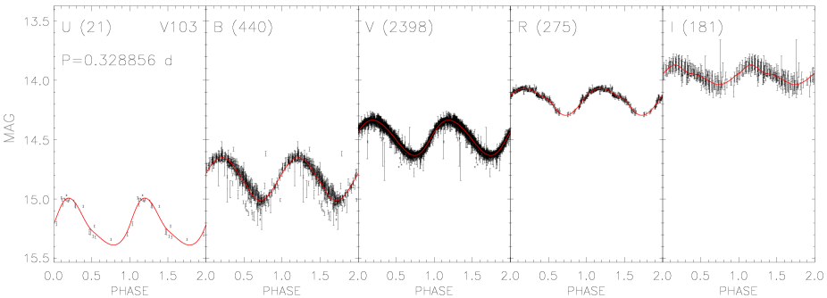
Figure 4: Same as Fig. 3, but for the RRc variable V103.

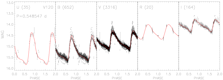
Figure 5: Same as Fig. 3, but for the candidate Blazhko variable V120.

Figure 10: Left: Same as Fig. 9, but zoomed on the RRL instability strip. The blue line shows the predicted First Overtone Blue Edge (FOBE), while the red one the predicted Fundamental Red Edge (FRE) of the instability strip (Marconi et al., 2015). Right: distribution of the V magnitudes of RRLs. The red curve shows the smoothed histogram. The four components of the multi-Gaussian fit are plotted in purple, while the black curve is the sum of the multi-Gaussian fit.

Figure 13: Panel a): Empirical dual-band Period-Wesenheit (PW) (V,B–V) relation for $\omega$ Cen RRLs. Light blue and red squares mark RRc and RRab variables. The light blue and the red lines display the linear fits, while the vertical bars show the standard deviations, $\sigma$, of the fits. The number of variables adopted in the fits are also labeled. Panel b): Same as panel a), but for the global (RRc$+$RRab) RRL sample. The periods of RRc variables were fundamentalized using $\log{P_{F}}=\log{P_{FO}}+0.127$. Panels c) and d): Same as a) and b), but for the PW(I,B–I) relation. Panels e) and f): Same as a) and b), but for the PW(I,V–I) relation. Panels g) and h): Same as a) and b), but for the triple-band PW(V,B–I) relation.

References

- Alonso-García et al. (2015) Alonso-García, J., Dékány, I., Catelan, M., et al. 2015, AJ, 149, 99
- Bailey (1902) Bailey, S. I. 1902, Annals of Harvard College Observatory, 38, 1
- Baird (1996) Baird, S. R. 1996, AJ, 112, 2132
- Beers et al. (1990) Beers, T. C., Flynn, K., & Gebhardt, K. 1990, AJ, 100, 32
- Bellini et al. (2009) Bellini, A., Piotto, G., Bedin, L. R., et al. 2009, A&A, 493, 959
- Bekki & Freeman (2003) Bekki, K., & Freeman, K. C. 2003, MNRAS, 346, L11
- Bellazzini et al. (2004) Bellazzini, M., Ferraro, F. R., Sollima, A., Pancino, E., & Origlia, L. 2004, A&A, 424, 199
- Benedict et al. (2011) Benedict, G. F., McArthur, B. E., Feast, M. W., et al. 2011, AJ, 142, 187
- Benkő et al. (2011) Benkő, J. M., Szabó, R., & Paparó, M. 2011, MNRAS, 417, 974
- Blažko (1907) Blažko, S. 1907, Astronomische Nachrichten, 175, 325
- Bono et al. (1997a) Bono, G., Caputo, F., Cassisi, S., Castellani, V., & Marconi, M. 1997a, ApJ, 479, 279
- Bono et al. (1997b) Bono, G., Caputo, F., Cassisi, S., Incerpi, R., & Marconi, M. 1997b, ApJ, 483, 811
- Bono et al. (1997c) Bono, G., Caputo, F., Castellani, V., & Marconi, M. 1997c, A&AS, 121, 327
- Bono & Marconi (1999) Bono, G., & Marconi, M. 1999, IAUS, 190, 527
- Bono et al. (2001) Bono, G., Caputo, F., Castellani, V., Marconi, M., & Storm, J. 2001, MNRAS, 326, 1183
- Bono (2003) Bono, G. 2003, ASPC, 298, 245
- Bono et al. (2003a) Bono, G., Caputo, F., Castellani, et al. 2003a, MNRAS, 344, 1097
- Bono et al. (2003b) Bono, G., Petroni, S., & Marconi, M. 2003b, ASPC, 292, 71
- Bono et al. (2008a) Bono, G., Caputo, F., Fiorentino, G., Marconi, M., & Musella, I. 2008a, ApJ, 684, 102
- Bono et al. (2008b) Bono, G., Stetson, P. B., Sanna, N., et al. 2008b, ApJ, 686, L87
- Bono et al. (2010) Bono, G., Stetson, P. B., VandenBerg, D. A., et al. 2010, ApJ, 708, L74
- Bono et al. (2016) Bono, G., Pietrinferni, A., Marconi, M., et al. 2016, Commmunications of the Konkoly Observatory Hungary, 105, 149
- Braga et al. (2015) Braga, V. F., Dall’Ora, M., Bono, G., et al. 2015, ApJ, 799, 165
- Brand & Wouterloot (1988) Brand, J., & Wouterloot, J. G. A. 1988, A&AS, 75, 117
- Buonanno et al. (1989) Buonanno, R., Corsi, C. E., & Fusi Pecci, F. 1989, A&A, 216, 80
- Cacciari et al. (2005) Cacciari, C., Corwin, T. M., & Carney, B. W. 2005, AJ, 129, 267
- Calamida et al. (2005) Calamida, A., Stetson, P. B., Bono, G., et al. 2005, ApJ, 634, L69
- Calamida et al. (2008) Calamida, A., Corsi, C. E., Bono, G., et al. 2008, ApJ, 673, L29
- Calamida et al. (2009) Calamida, A., Bono, G., Stetson, P. B., et al. 2009, ApJ, 706, 1277
- Caputo (1990) Caputo, F. 1990, A&A, 239, 137
- Cardelli et al. (1989) Cardelli, J. A., Clayton, G. C., & Mathis, J. S. 1989, ApJ, 345, 245
- Carretta et al. (2009) Carretta, E., Bragaglia, A., Gratton, R. G., et al. 2009, A&A, 505, 117
- Castellani & Quarta (1987) Castellani, V., & Quarta, M. L. 1987, A&AS, 71, 1
- Castellani et al. (2006) Castellani, V., Iannicola, G., Bono, G., et al. 2006, A&A, 446, 569
- Castellani et al. (2007) Castellani, V., Calamida, A., Bono, G., et al. 2007, ApJ, 663, 1021
- Catelan (2004a) Catelan, M. 2004a, ApJ, 600, 409
- Catelan (2004b) Catelan, M. 2004b, ASPC, 310, 113
- Catelan et al. (2004) Catelan, M., Pritzl, B. J., & Smith, H. A. 2004, ApJS, 154, 633
- Clement & Rowe (2000) Clement, C. M., & Rowe, J. 2000, AJ, 120, 2579
- Clement et al. (2001) Clement, C. M., Muzzin, A., Dufton, Q., et al. 2001, AJ, 122, 2587
- Coppola et al. (2015) Coppola, G., Marconi, M., Stetson, P. B., et al. 2015, ApJ, 814, 71
- Cox et al. (1983) Cox, A.N., Hodson, S.W., Clancy, S.P. 1983, ApJ, 266, 94
- D’Antona et al. (2005) D’Antona, F., Bellazzini, M., Caloi, V., et al. 2005, ApJ, 631, 868
- Da Costa & Coleman (2008) Da Costa, G. S., & Coleman, M. G. 2008, AJ, 136, 506
- Dall’Ora et al. (2003) Dall’Ora, M., Ripepi, V., Caputo, F., et al. 2003, AJ, 126, 197
- Del Principe et al. (2006) Del Principe, M., Piersimoni, A. M., Storm, J., et al. 2006, ApJ, 652, 362
- Di Cecco et al. (2010) Di Cecco, A., Bono, G., Stetson, P. B., et al. 2010, ApJ, 712, 527
- Di Criscienzo et al. (2004) Di Criscienzo, M., Marconi, M., & Caputo, F. 2004, ApJ, 612, 1092
- Di Criscienzo et al. (2011) Di Criscienzo, M., Greco, C., Ripepi, V., et al. 2011, AJ, 141, 81
- Dickens & Caldwell (1988) Dickens, R. J., & Caldwell, S. P. 1988, MNRAS, 233, 677
- Drake et al. (2009) Drake, A.J. et al. 2009, ApJ, 696, 870
- Drake et al. (2013a) Drake, A. J., Catelan, M., Djorgovski, S. G., et al. 2013a, ApJ, 763, 32
- Drake et al. (2013b) Drake, A. J., Catelan, M., Djorgovski, S. G., et al. 2013b, ApJ, 765, 154
- Drake et al. (2014) Drake, A. J., Graham, M. J., Djorgovski, S. G., et al. 2014, ApJS, 213, 9
- D’Souza & Rix (2013) D’Souza, R., & Rix, H.-W. 2013, MNRAS, 429, 1887
- Fabrizio et al. (2011) Fabrizio, M., Nonino, M., Bono, G., et al. 2011, PASP, 123, 384
- Fabrizio et al. (2015) Fabrizio, M., Nonino, M., Bono, G., et al. 2015, A&A, 580, A18
- Fernández-Trincado et al. (2015a) Fernández-Trincado, J. G., Vivas, A. K., Mateu, C. E., et al. 2015a, A&A, 574, A15
- Fernández-Trincado et al. (2015b) Fernández-Trincado, J. G., Robin, A. C., Vieira, K., et al. 2015b, A&A, 583, A76
- Fiorentino et al. (2015) Fiorentino, G., Bono, G., Monelli, M., et al. 2015, ApJ, 798, L12
- Fitzpatrick & Massa (2007) Fitzpatrick, E.L., & Massa, D. 2007, ApJ, 663, 320
- Fraix-Burnet & Davoust (2015) Fraix-Burnet, D., & Davoust, E. 2015, MNRAS, 450, 3431
- Freeman (1993) Freeman, K. C. 1993, APSC, 48, 608
- Gratton et al. (2003) Gratton, R. G., Carretta, E., Claudi, R., Lucatello, S., & Barbieri, M. 2003, A&A, 404, 187
- Harris (1996) Harris, W. E. 1996, AJ, 112, 1487
- Inno et al. (2015) Inno, L., Matsunaga, N., Romaniello, M., et al. 2015, A&A, 576, A30
- Iben & Huchra (1971) Iben, I., Jr., & Huchra, J. 1971, A&A, 14, 293
- Jang & Lee (2015) Jang, I. S., & Lee, M. G. 2015, ApJ, 807, 133
- Johnson et al. (2009) Johnson, C. I., Pilachowski, C. A., Michael Rich, R., & Fulbright, J. P. 2009, ApJ, 698, 2048
- Johnson & Pilachowski (2010) Johnson, C. I., & Pilachowski, C. A. 2010, ApJ, 722, 1373
- Jones et al. (1996) Jones, R. V., Carney, B. W., & Fulbright, J. P. 1996, PASP, 108, 877
- Jurcsik et al. (2001) Jurcsik, J., Clement, C., Geyer, E. H., & Domsa, I. 2001, AJ, 121, 951
- Jurcsik et al. (2012) Jurcsik, J., Hajdu, G., Szeidl, B., et al. 2012, MNRAS, 419, 2173
- Jurcsik et al. (2015) Jurcsik, J., Smitola, P., Hajdu, G., et al. 2015, ApJS, 219, 25
- Kaluzny et al. (2002) Kaluzny, J., Thompson, I., Krzeminski, W., et al. 2002, Omega Centauri, A Unique Window into Astrophysics, 265, 155
- Kaluzny et al. (2004) Kaluzny, J., Olech, A., Thompson, I. B., et al. 2004, A&A, 424, 1101
- Kaluzny et al. (2007) Kaluzny, J., Rucinski, S. M., Thompson, I. B., Pych, W., & Krzeminski, W. 2007, AJ, 133, 2457
- Kaluzny et al. (1997) Kaluzny, J., Kubiak, M., Szymanski, M., et al. 1997, A&AS, 125, 343
- King & Anderson (2002) King, I. R., & Anderson, J. 2002, ASPC, 265, 21
- Kirby et al. (2013) Kirby, E. N., Cohen, J. G., Guhathakurta, P., et al. 2013, ApJ, 779, 102
- Kunder et al. (2013a) Kunder, A., Stetson, P. B., Catelan, M., Walker, A. R., & Amigo, P. 2013a, AJ, 145, 33
- Kunder et al. (2013b) Kunder, A., et al. 2013b, AJ, 146, 119
- Landolt (1983) Landolt, A. U. 1983, AJ, 88, 439
- Landolt (1992) Landolt, A. U. 1992, AJ, 104, 340
- Latour et al. (2014) Latour, M., Randall, S. K., Fontaine, G., et al. 2014, ApJ, 795, 106
- Lee et al. (1993) Lee, M. G., Freedman, W. L., & Madore, B. F. 1993, ApJ, 417, 553
- Longmore et al. (1990) Longmore, A. J., Dixon, R., Skillen, I., Jameson, R. F., & Fernley, J. A. 1990, MNRAS, 247, 684
- Lub (2002) Lub, J. 2002, ASPC, 265, 95
- Lub (2016) Lub, J. 2016, Commmunications of the Konkoly Observatory Hungary, 105, 39
- Madore (1982) Madore, B. F. 1982 ApJ, 253, 575
- Majewski et al. (2012) Majewski, S. R., Nidever, D. L., Smith, V. V., et al. 2012, ApJ, 747, L37
- Marconi et al. (2011) Marconi, M., Bono, G., Caputo, F., et al. 2011, ApJ, 738, 111
- Marconi et al. (2014) Marconi, M., Musella, I., Di Criscienzo, M., et al. 2014, MNRAS, 444, 3809
- Marconi et al. (2015) Marconi, M., Coppola, G., Bono, G., et al. 2015, ApJ, 808, 50
- Martin (1938) Martin, W. C. 1938, Annalen van de Sterrewacht te Leiden, 17, 1
- Martínez-Vázquez et al. (2015) Martínez-Vázquez, C. E., Monelli, M., Bono, G., et al. 2015, MNRAS, 454, 1509
- McConnachie (2012) McConnachie, A. W. 2012, AJ, 144, 4
- McNamara (2011) McNamara, D. H. 2011, AJ, 142, 110
- Monelli et al. (2005) Monelli, M., Corsi, C. E., Castellani, V., et al. 2005, ApJ, 621, L117
- Monet et al. (1998) Monet, D. G., et al. 1998, USNO-A2.0 (Washington: US Nav. Obs.)
- Moni Bidin et al. (2012) Moni Bidin, C., Villanova, S., Piotto, G., et al. 2012, A&A, 547, A109
- Navarrete et al. (2015) Navarrete, C., Contreras Ramos, R., Catelan, M., et al. 2015, A&A, 577, A99
- Navarrete et al. (2016) Navarrete, C., Catelan, M., Contreras Ramos, R., Gran, F., & Alonso-Garcia, J. 2016, Commmunications of the Konkoly Observatory Hungary, 105, 45
- Norris & Da Costa (1995) Norris, J. E., & Da Costa, G. S. 1995, ApJ, 447, 680
- Norris et al. (1996) Norris, J. E., Freeman, K. C., & Mighell, K. J. 1996, ApJ, 462, 241
- Olech & Moskalik (2009) Olech, A., & Moskalik, P. 2009, A&A, 494, L17
- Oosterhoff (1939) Oosterhoff, P. T. 1939, The Observatory, 62, 104
- Pancino et al. (2002) Pancino, E., Pasquini, L., Hill, V., Ferraro, F. R., & Bellazzini, M. 2002, ApJ, 568, L101
- Pietrinferni et al. (2006) Pietrinferni, A., Cassisi, S., Salaris, M., Castelli, F. 2006, ApJ, 642, 797
- Pietrzyński et al. (2013) Pietrzyński, G., Graczyk, D., Gieren, W., et al. 2013, Nature, 495, 76
- Pritzl et al. (2001) Pritzl, B. J., Smith, H. A., Catelan, M., & Sweigart, A. V. 2001, AJ, 122, 2600
- Pritzl et al. (2002) Pritzl, B. J., Smith, H. A., Catelan, M., & Sweigart, A. V. 2002, AJ, 124, 949
- Pritzl et al. (2003) Pritzl, B. J., Smith, H. A., Stetson, P. B., et al. 2003, AJ, 126, 1381
- Randall et al. (2011) Randall, S. K., Calamida, A., Fontaine, G., Bono, G., & Brassard, P. 2011, ApJ, 737, L27
- Renzini & Sweigart (1980) Renzini, A., & Sweigart, A. V. 1980, Current Problems in Stellar Pulsation Instabilities, 271
- Rey et al. (2000) Rey, S.-C., Lee, Y.-W., Joo, J.-M., Walker, A., & Baird, S. 2000, AJ, 119, 1824
- Rood (1973) Rood, R.T. 1973, AJ, 184, 815
- Salaris et al. (2013) Salaris, M., de Boer, T., Tolstoy, E., Fiorentino, G., & Cassisi, S. 2013, A&A, 559, A57
- Savino et al. (2015) Savino, A., Salaris, M., & Tolstoy, E. 2015, A&A, 583, A126
- Sawyer Hogg (1973) Sawyer Hogg, H. 1973, Publications of the David Dunlap Observatory, 3, 1
- Scargle (1982) Scargle, J. D. 1982, ApJ, 263, 835
- Schlegel et al. (1998) Schlegel, D. J., Finkbeiner, D. P., & Davis, M. 1998, ApJ, 500, 525
- Smith (1981) Smith, H. A., PASP, 93, 721
- Smith et al. (2000) Smith, V. V., Suntzeff, N. B., Cunha, K., et al. 2000, AJ, 119, 1239
- Smith et al. (2011) Smith, H. A., Catelan, M., & Kuehn, C. 2011, in RR Lyrae Stars, Metal-Poor Stars, and the Galaxy, 5, 17
- Sollima et al. (2006a) Sollima, A., Borissova, J., Catelan, M., et al. 2006a, ApJ, 640, L43
- Sollima et al. (2006b) Sollima, A., Cacciari, C., & Valenti, E. 2006b, MNRAS, 372, 1675
- Sollima et al. (2008) Sollima, A., Cacciari, C., Arkharov, A.A.H., et al. 2008, MNRAS, 384, 1583
- Sollima et al. (2014) Sollima, A., Cassisi, S., Fiorentino, G., et al. 2014, MNRAS, 444, 1862
- Soszyński et al. (2005) Soszyński, I., Gieren, W., & Pietrzyński, G. 2005, PASP, 117, 823
- Soszyński et al. (2009) Soszyński, I., Udalski, A., Szymański, M. K., et al. 2009, Acta Astron., 59, 1
- Soszyński et al. (2011) Soszyński, I., Udalski, A., Pietrukowicz, P., et al. 2011, Acta Astron., 61, 285
- Stetson (1996) Stetson, P. B. 1996, PASP, 108, 851
- Stetson et al. (1998a) Stetson, P. B., Saha, A., Ferrarese, L., et al. 1998, ApJ, 508, 491
- Stetson et al. (1998b) Stetson, P. B., Hesser, J. E., & Smecker-Hane, T. A. 1998, PASP, 110, 533
- Stetson (1994) Stetson, P. B., PASP, 106, 250
- Stetson (2000) Stetson, P. B., PASP, 112, 925
- Stetson (2005) Stetson, P. B., PASP, 117, 563
- Stetson et al. (2014a) Stetson, P. B., Braga, V. F., Dall’Ora, M., et al. 2014a, PASP, 126, 521
- Stetson et al. (2014b) Stetson, P. B., Fiorentino, G., Bono, G., et al. 2014b, PASP, 126, 616
- Sturch (1978) Sturch, C. R. 1978, PASP, 90, 264
- Suntzeff & Kraft (1996) Suntzeff, N. B., & Kraft, R. P. 1996, AJ, 111, 1913
- Tailo et al. (2016) Tailo, M., Di Criscienzo, M., D’Antona, F., Caloi, V., & Ventura, P. 2016, MNRAS, 457, 4525
- Thompson et al. (2001) Thompson, I. B., Kaluzny, J., Pych, W., et al. 2001, AJ, 121, 3089
- Torrealba et al. (2015) Torrealba, G., Catelan, M., Drake, A. J., et al. 2015, MNRAS, 446, 2251
- Udalski et al. (1999) Udalski, A., Szymanski, M., Kubiak, M., et al. 1999, Acta Astron., 49, 201
- van Gent (1948) van Gent, H. 1948, Bull. Astron. Inst. Netherlands, 10, 377
- van Leeuwen et al. (2000) van Leeuwen, F., Le Poole, R. S., Reijns, R. A., Freeman, K. C., & de Zeeuw, P. T. 2000, A&A, 360, 472
- van de Ven et al. (2006) van de Ven, G., van den Bosch, R. C. E., Verolme, E. K., & de Zeeuw, P. T. 2006, A&A, 445, 513
- Van den Bergh (1975) Van den Bergh, S. 1975, Stars and Stellar Systems, 9, 509. Ed. A. Sandage, M. Sandage, and J. Kristian (University of Chicago Press)
- Vanture et al. (2002) Vanture, A. D., Wallerstein, G., & Suntzeff, N. B. 2002, ApJ, 569, 984
- Wallerstein et al. (2009) Wallerstein, G., Kovtyukh, V. V., & Andrievsky, S. M. 2009, ApJ, 692, L127
- Watkins et al. (2013) Watkins, L. L., van de Ven, G., den Brok, M., & van den Bosch, R. C. E. 2013, MNRAS, 436, 2598
- Welch & Stetson (1993) Welch, D. L., & Stetson, P. B. 1993, AJ, 105, 1813
- Weldrake et al. (2007) Weldrake, D. T. F., Sackett, P. D., & Bridges, T. J. 2007, AJ, 133, 1447
- Wilkens (1965) Wilkens, H. 1965, Boletin de la Asociacion Argentina de Astronomia La Plata Argentina, 10, 66
- Zinn & West (1984) Zinn, R., & West, M. J. 1984, ApJS, 55, 45
- Zinnecker et al. (1988) Zinnecker, H., Keable, C. J., Dunlop, J. S., et al. 1988, IAUS, 126, 603