Asset Pricing in a Semi-Markov Modulated Market with Time-dependent Volatility

Coordinator Dr. Anindya Goswami Assistant Professor Department of Mathematics Prof. M. K. Ghosh This thesis is dedicated to my parents. 2016 April

Introduction

In 1973, Black, Scholes and Merton developed a mathematical model for the problem of option pricing, for which they were awarded the Nobel prize in Economics. Since then, numerous different improvements of their theoretical model are being studied. Regime switching models are one such extension of the Black-Scholes model. The goal of this project is to establish the pricing theory of defaultable bonds for a very general kind of regime switching market. Extensive research has been done to study markets with Markov-modulated regime switching. However, it seems that the above problem with semi-Markov regimes has not yet been studied in the literature. A semi-Markov switching has past memory unlike the well studied homogeneous Markov switching which is memoryless. Hence the former has much greater appeal in terms of applicability than the latter. The semi-Markov switching is mathematically more interesting, too, mainly because of non-locality and unboundedness of the infnitesimal generator of the related augmented process. To address this problem, a satisfactory knowledge of continuous time stochastic processes, in particular diffusion processes and Poisson point processes, is necessary. A reasonable understanding of pricing theory in continuous time market model is also essential.

We have successfully represented a large class of semi-Markov processes as solutions of a class of stochastic integral equations. This finding is original in nature and crucial to achieve the main aim of the project.

In the geometric Brownian motion model of asset prices, the drift and the volatility coefficients of the prices are constants. On the other hand, the regime switching model, allows those coefficients to be Markov pure jump processes. We consider a financial market where the asset price dynamics follow a regime switching model where the coefficients depend on a more general, possibly non-Markov pure jump stochastic processes. We further allow the volatility coefficient to depend on time explicitly, to capture periodic fluctuations like Monday effects etc. Under this market assumption we study locally risk minimizing pricing of vanilla options. It is shown that the price function can be obtained by solving a non-local degenerate parabolic PDE. We establish existence and uniqueness of a classical solution of at most linear growth of the PDE. We further show that the PDE is equivalent to a Volterra integral equation of second kind. Thus one can find the price function by solving the integral equation which is computationally more efficient. We finally show that the corresponding optimal hedging can be computed by performing a numerical integration.

Chapter 1 Preliminaries

Definition 1.0.1.

Let $(E,\mathcal{E})$ be an Euclidean measurable space. Let $M_{P}(E)$ be the set of all integer-valued measures on $(E,\mathcal{E})$. We associate $M_{P}(E)$ with a $\sigma$-algebra $\mathcal{M}_{P}(E)$, which is the smallest $\sigma$-algebra on $M_{P}(E)$ that makes the maps $A:M_{P}(E)\rightarrow\mathbb{N}\cup\{0\}$, $m\mapsto m(A)$ measurable for all Borel sets $A$. Let $\mu$ be a Radon measure on $E$. A Poisson random measure with mean measure $\mu$ is a measurable function $\wp:(\Omega,\mathcal{F},P)\rightarrow(M_{P}(E),\mathcal{M}_{P}(E))$ satisfying the following properties:

1. For $A\in\mathcal{E}$ and $k\in\mathbb{N}$,

   $$P[\omega:\wp(\omega)(A)=k]=\begin{cases}e^{-\mu(A)}\frac{(\mu(A))^{k}}{k!},\ &\mu(A)<\infty\\ 0,\ &\mu(A)=\infty.\end{cases}$$ (1.1)

2. For any $m\in\mathbb{N}$, if $A_{1},A_{2},\dots,A_{m}$ are mutually disjoint sets in $\mathcal{E}$, then $\wp(A_{1}),\wp(A_{2}),$
   $\dots,\wp(A_{m})$ are independent random variables.

Definition 1.0.2.

A discrete-time Markov chain is a sequence of random variables $\{X_{n}\}_{n\geq 0}$ satisfying

$$P[X_{n+1}=x\mid X_{0}=x_{0},X_{1}=x_{1},\dots X_{n}=x_{n}]=P[X_{n+1}=x\mid X_{n}=x_{n}],$$

provided both conditional probabilities are well-defined, i.e $P[X_{0}=x_{0},X_{1}=x_{1},\dots X_{n}=x_{n}]>0$.

Definition 1.0.3.

A continuous-time time-homogeneous Markov chain with rate matrix $\Lambda$ is a stochastic process $\{X_{t}\}_{t\geq 0}$ satisfying the following conditions

1. $X_{t}$ is a piecewise constant right-continuous process with left-limits, with discontinuities at a discrete set $\{T_{n}\}_{n\geq 1}$. (This means that $X_{t}$ is a right-continuous process whose left-hand limit exists at all points with probability 1.)

2. The sequence $\{X_{T_{n}}\}_{n=0,1,\dots}$ is a Markov chain with transition matrix $\mathbb{P}=(p_{ij})$, where $p_{ij}=\frac{\lambda_{ij}}{|\lambda_{ii}|}$.

3. $P\left[X_{T_{n+1}}=j,T_{n+1}-T_{n}\leq y|(X_{0},T_{0}),(X_{1},T_{1}),\dots,(X_{T_{n}}=i,T_{n})\right]=p_{ij}(1-e^{\lambda_{ii}y})$.

Definition 1.0.4.

A general continuous-time Markov process is a process $\{X_{t}\}_{t\geq 0}$ on a probability space $(\Omega,\mathcal{F},P)$ and taking values in a measurable space $(S,\mathcal{S})$, satisfying

$$P[X_{t}\in A\mid\mathcal{F}_{s}]=P[X_{t}\in A\mid X_{s}]$$ (1.2)

for all $A\in\mathcal{S}$ and for each $s<t$.

Definition 1.0.5.

A semi-Markov process is a process $\{X_{t}\}_{t\geq 0}$ that satisfies the following properties:

1. $X_{t}$ is a piecewise constant rcll process with discontinuities at a discrete set $\{T_{n}\}_{n\geq 1}$.

2. The transition probabilities satisfy

   $$P\left[X_{T_{n+1}}=j,T_{n+1}-T_{n}\leq y|(X_{0},T_{0}),(X_{1},T_{1}),\dots,(X_{T_{n}},T_{n})\right]$$

   $$= P\left[X_{T_{n+1}}=j,T_{n+1}-T_{n}\leq y|X_{T_{n}}\right].$$ (1.3)

Definition 1.0.6.

A $C_{0}$-semigroup of operators $\{S(t)\}_{t\geq 0}$ on a Banach space $V$ is a map $S:\mathbb{R}_{+}\rightarrow BL(V)$, such that

1. $S_{0}f=f\quad\forall f\in V$,

2. $S_{t+s}=S_{t}\circ S_{s}\quad\forall t,s\geq 0$, and

3. $\|S_{t}f-f\|\rightarrow 0$ as $t\downarrow 0$, for all $f\in V$.

Definition 1.0.7.

Let $\{S(t)\}_{t\geq 0}$ be a $C_{0}$-semigroup of operators. The domain of the infinitesimal generator of the semigroup is defined as

$$\mathcal{D}(\mathcal{A}):=\left\{f\in V\mid\lim_{t\rightarrow 0}\frac{S_{t}f-f}{t}\textrm{ exists}\right\}$$

and the infinitesimal generator of $f$ is the operator $\mathcal{A}$, defined such that

$$\mathcal{A}f:=\lim_{t\rightarrow 0}\frac{S_{t}f-f}{t}$$

for all $f\in\mathcal{D}$.

Chapter 2 Age-dependent processes

2.1 Time-homogeneous Age-dependent processes

We consider a class of stochastic processes which is constructed as a strong solution of a certain set of stochastic integral equations. Let $(\Omega,\mathcal{F},\{\mathcal{F}_{t}\}_{t\geq 0},P)$ be a filtered probability space, and $\chi=\left\{1,2,\dots,k\right\}\subset\mathbb{R}$ be the state space. For $i,j\in\chi$ and $i\neq j$, define

$$\lambda:\chi\times\chi\times\ (0,\infty)\rightarrow[0,\infty)$$ (2.1)

to be a measurable function with

$$\sup_{y\in(0,\infty)}\sum_{j\neq i}\lambda_{ij}(y)<\infty.$$ (2.2)

and

$$\lim\limits_{y\rightarrow\infty}\Lambda_{i}(y)=\infty,\text{\ where\ }\Lambda_{i}(y)=\int_{0}^{y}\sum_{j\neq i}\lambda_{ij}(v)\,dv.$$ (2.3)

The diagonal elements are defined as $\lambda_{ii}(y):=-\sum_{j\neq i}\lambda_{ij}(y)$.

For $i\neq j,y>0$, let $\Lambda_{ij}(y)$ be consecutive (w.r.t the lexicographical ordering) right-open, left-closed intervals of length $\lambda_{ij}(y)$. Define $h:\ \chi\times\mathbb{R}_{+}\times\mathbb{R}\rightarrow\mathbb{R}$ as

$$h(i,y,z)=\sum_{j\neq i\in\chi}(j-i)\mathds{1}_{\Lambda_{ij}(y)}(z)$$ (2.4)

and a function $g:\ \chi\times\mathbb{R}_{+}\times\mathbb{R}\rightarrow\mathbb{R}$ as

$$g(i,y,z)=y\sum_{j\neq i\in\chi}\mathds{1}_{\Lambda_{ij}(y)}(z).$$ (2.5)

.

We consider the following system of coupled stochastic integral equations in $X_{t}$ and $Y_{t}$:

$$X_{t}=X_{0}+\int_{(0,t]}\int_{\mathbb{R}}h(X_{u-},Y_{u-},z)\,\wp(du,dz)$$ (2.6)

$$Y_{t}=Y_{0}+t-\int_{(0,t]}\int_{\mathbb{R}}g(X_{u-},Y_{u-},z)\,\wp(du,dz),$$ (2.7)

where $h$ and $g$ are defined by equations (2.4) and (2.5) respectively, $\wp(du,dz)$ is a Poisson random measure on $\mathbb{R}_{+}\times\mathbb{R}$ with intensity $du\times dz$, and $\{\wp((0.t]\times dz)\}_{t\geq 0}$ is adapted to the filtration $\{\mathcal{F}_{t}\}_{t\geq 0}$.

Theorem 2.1.1.

There exists a unique strong solution to equations (2.6) and (2.7).

Proof. First, we note that (2.2) can be rewritten as:

$$\sum_{j\neq i}\lambda_{ij}(y)<c\ \text{for all }y\in[0,\infty),$$ (2.8)

for some $c>0$. Thus, it follows that

$$\bigcup_{y\in(0,T]}\left[\{y\}\times[0,\sum_{j\neq i}\lambda_{ij}(y)]\right]\subset[0,T]\times[0,c].$$

The interval $[0,c]$ has finite Lebesgue measure $c$. Define $D$ to be the set of all point masses of the measure $\wp(\omega)$:

$$D:=\left\{s\in(0,\infty)|\wp(\omega)(\{s\}\times[0,c])=1\right\}\text{ for any fixed $\omega\in\Omega$}.$$

An illustration of a sample of the points of a Poisson random measure with $c=10$ and $T=1$ is shown in Figure 2.1.

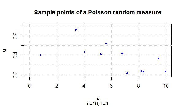
Figure 2.1: A sample of point masses of a Poisson random measure

The set of all transition times of $X(\omega)$ is a subset of $D$. Since the measure of the set $[0,c]$ is finite, $D$ is a discrete set (i.e, $D$ has no limit point) with probability 1. We can thus enumerate the set $D$ as

$$D=\{0,\sigma_{1},\sigma_{2},\dots,\},$$

and it is easy to see that $\sigma_{1},\sigma_{2},\dots$ are stopping times under the filtration $\mathcal{F}_{t}$ of the underlying probability space. Since $D$ is a discrete set,

$$\lim_{n\rightarrow\infty}\sigma_{n}=\infty\ \text{a.s.}$$ (2.9)

We use an iterative argument for proving the existence and uniqueness of a strong solution to (2.6) and (2.7). For a fixed $\omega$, we construct a solution to this pair of equations on the time interval $[0,\sigma_{1}]$. Then we extend this solution to the time interval $(\sigma_{1},\sigma_{2}]$, and so on.

Since

$$\wp(\omega)([0,\sigma_{1})\times[0,c])=0,$$

for $t\in[0,\sigma_{1})$,

$$X_{t}(\omega) =X_{0}+\int_{0}^{t}\int_{[0,c]}h(X_{u-},Y_{u-},z)\,\wp(\omega)(du,dz)$$

$$=X_{0}$$

and

$$Y_{t}(\omega) =Y_{0}+t-\int_{0}^{t}\int_{[0,c]}g(X_{u-},Y_{u-},z)\,\wp(\omega)(du,dz)$$

$$=Y_{0}+t.$$

At $t=\sigma_{1}$,

$$X_{\sigma_{1}}(\omega) =X_{0}+\int_{[0,c]}h(X_{0},Y_{0}+\sigma_{1},z)\,\wp(\omega)(\{\sigma_{1}\}\times dz),$$

$$Y_{\sigma_{1}}(\omega) =Y_{0}+\sigma_{1}-\int_{[0,c]}g(X_{0},Y_{0}+\sigma_{1},z)\,\wp(\omega)(\{\sigma_{1}\}\times dz).$$

Since we have been able to write down the solution in the time interval $[0,\sigma_{1}]$ explicitly, it is obviously unique.

Now we consider the time interval $(\sigma_{1},\sigma_{2}]$. We define the following quantities:

$$\tilde{X}(0) =X(\sigma_{1}),$$

$$\tilde{Y}(0) =Y(\sigma_{1}),$$

$$\tilde{\wp}(ds,dz) =\wp(\sigma_{1}+ds,dz),$$

$$\tilde{\sigma}_{n} =\sigma_{n+1}-\sigma_{1}.$$

Then, $\tilde{D}=\left\{s>0|s+\sigma_{1}\in D\right\}=\{\tilde{\sigma}_{n}\}_{n\geq 1}.$ Now we consider the equations (2.6) and (2.7) on $[0,\tilde{\sigma_{1}}]$, where $X_{0},Y_{0}$ and $\wp$ are replaced by $\tilde{X}(0),\tilde{Y}(0)$ and $\tilde{\wp}$ respectively. If $t\in[0,\tilde{\sigma_{1}})$, then the solution $\tilde{X}_{t}$ is given by

$$\tilde{X}_{t} =\tilde{X}_{0},$$

$$\tilde{Y}_{t} =\tilde{Y}_{0}+t.$$

and for $t=\tilde{\sigma}_{1}$, we have:

$$\tilde{X}_{\tilde{\sigma}_{1}} =\tilde{X}_{0}+\int_{[0,c]}h(\tilde{X}_{0},\tilde{Y}_{0}+\tilde{\sigma}_{1},z)\,\tilde{\wp}(\{\tilde{\sigma}_{1}\}\times dz),$$

$$\tilde{Y}_{\tilde{\sigma}_{1}} =\tilde{Y}_{0}+\tilde{\sigma}_{1}-\int_{[0,c]}g(\tilde{X}_{0},\tilde{Y}_{0}+\tilde{\sigma}_{1},z)\,\tilde{\wp}(\{\tilde{\sigma}_{1}\}\times dz).$$

Therefore, the solution $(X,Y)$ of the original equations can be reconstructed from $(\tilde{X},\tilde{Y})$ by the following relation

$$X_{t} =\begin{cases}X(t),\ t\in[0,\sigma_{1}]\\ \tilde{X}(t-\sigma_{1}),\ t\in(\sigma_{1},\sigma_{2}]\end{cases}$$

$$Y_{t} =\begin{cases}Y(t),\ t\in[0,\sigma_{1}]\\ \tilde{Y}(t-\sigma_{1}),\ t\in(\sigma_{1},\sigma_{2}].\end{cases}$$

This establishes the existence and uniqueness of the strong solution in the time interval $[0,\sigma_{2}]$.

Continuing in this fashion, we can uniquely construct the solution in successive time intervals. By (2.9), this sequence of intervals covers the entire positive real time-axis. Hence, the solution is globally determined. ∎

In the above proof, it is evident that the process $X_{t}$ has almost surely piecewise constant r.c.l.l paths. The points of discontinuity of $X_{t}$ are called transition times.

Definition 2.1.1.

Transition times are elements of an increasing sequence $\{T_{n}\}_{n\geq 1}$ such that $\{T_{n}:n\geq 1\}=\{t>0:X_{t}\neq X_{t-}\}$. We set $T_{0}:=-Y_{0}$. We define the holding times $\tau_{n}:=T_{n}-T_{n-1}$ for all $n\geq 1$.

From the above definitions, it is clear that

$$X_{u}-X_{u-}=\int_{\mathbb{R}}h(X_{u-},Y_{u-},z)\,\wp(\{u\}\times dz)$$

is non-zero if and only if $u=T_{n}$ for some positive integer $n$. This also implies that

$$\int_{\mathbb{R}}g(X_{u-},Y_{u-},z)\,\wp(\{u\}\times dz)=\begin{cases}Y_{u-},\text{ if $u=T_{n}$ for some $n$}\\ 0,\text{ otherwise}.\end{cases}$$

Hence, by induction, we obtain, for any integer $n\geq 0$,

$$Y_{t}=Y_{0}+t-\sum_{r=1}^{n}Y_{T_{r}-}\text{ for }t\in[T_{n},T_{n+1}).$$

Thus, $Y_{t}=0$ iff $t=T_{n}$ for some $n\in\mathbb{N}$, and $Y_{T_{n}-}=T_{n}-T_{n-1}$ for all $n\in\mathbb{N}$. This observation motivates us to define the following:

Definition 2.1.2.

Let $(X_{t},Y_{t})$ be the unique strong solution to equations (2.6) and (2.7). The process $X_{t}$ is then called an “age-dependent process” and $Y_{t}$ is called the “holding time process” corresponding to $X_{t}$.

Theorem 2.1.2.

Let $(X_{t},Y_{t})$ be the unique strong solution to equations (2.6) and (2.7). The process $Z_{t}:=(X_{t},Y_{t})$ is a Markov process.

Proof.  From equations (2.6) and (2.7), we get, for $t<T$,

$${X}_{T} ={X}_{0}+\int_{0}^{T}\int_{\mathbb{R}}h({X}_{u-},{Y}_{u-},z)\,{\wp}(du,dz)$$

$$={X}_{t}+\int_{t}^{T}\int_{\mathbb{R}}h({X}_{u-},{Y}_{u-},z)\,{\wp}(du,dz)$$

and

$${Y}_{T} =Y_{0}+T-\int_{0}^{T}\int_{\mathbb{R}}g({X}_{u-},{Y}_{u-},z)\,{\wp}(du,dz)$$

$$={Y}_{t}+(T-t)-\int_{t}^{T}\int_{\mathbb{R}}g({X}_{u-},{Y}_{u-},z)\,{\wp}(du,dz).$$

From the second property of $\wp$, as in Definition 1.0.1 and from the above expressions, it is thus clear that $Z_{t}$ is a Markov process.∎

It is also easy to see that $Z_{t}$ is strongly Markov.

Theorem 2.1.3.

Let $X_{t}$ be an age-dependent process. Then, $X_{t}$ is a semi-Markov process.

Proof. We have already seen in the proof of Theorem 2.1.1, that $X_{t}$ is a piecewise constant right-continuous process, and the left-hand limits exist. In other words, $X_{t}$ is a càdlàg process.

Next, we show that

$$P[X_{T_{n+1}}=j,T_{n+1}-T_{n}\leq y\mid(X_{T_{0}},{T_{0}}),(X_{T_{1}},{T_{1}}),\dots,(X_{T_{n}},{T_{n}})].$$

$$= P[X_{T_{n+1}}=j,T_{n+1}-T_{n}\leq y\mid X_{T_{n}}].$$ (2.10)

We note that the LHS of (2.10) can be written as

$$P(X_{T_{n+1}}=j\mid(X_{T_{0}},{T_{0}}),(X_{T_{1}},{T_{1}}),\dots,(X_{T_{n}},{T_{n}}),\{T_{n+1}-T_{n}\leq y\})\times$$

$$P[T_{n+1}-T_{n}\leq y\mid(X_{T_{0}},{T_{0}}),(X_{T_{1}},{T_{1}}),\dots,(X_{T_{n}},{T_{n}})]$$ (2.11)

From equation (2.6),

$$X_{T_{n+1}}=X_{T_{n}}+\int_{\mathbb{R}}h(X_{T_{n}},T_{n+1}-T_{n},z)\,\wp(\{T_{n}+(T_{n+1}-T_{n})\}\times dz),$$

since $Y_{T_{n+1}\!-}=T_{n+1}-T_{n}$ and

$$\int_{(T_{n},T_{n+1})}\int_{\mathbb{R}}h(X_{u-},Y_{u-},z)\,\wp(du,dz)=0.$$

Again, since $\wp$ is a Poisson random measure, for any Borel set $B\subset(0,\infty)\times\mathbb{R}$, $\wp((T_{n},0)+B)$ is independent of $\mathcal{F}_{T_{n}}$. Therefore,

$$P(X_{T_{n+1}}=j\mid(X_{T_{0}},{T_{0}}),(X_{T_{1}},{T_{1}}),\dots,(X_{T_{n}},{T_{n}}),\{T_{n+1}-T_{n}\leq y\})$$

$$= P\bigg{(}\int_{\mathbb{R}}h(X_{T_{n}},T_{n+1}-T_{n},z)\,\wp(\{T_{n}+(T_{n+1}-T_{n})\}\times dz)=j-X_{T_{n}}\Big{|}\bigg{.}$$

$$\bigg{.}(X_{T_{0}},{T_{0}}),(X_{T_{1}},{T_{1}}),\dots,(X_{T_{n}},{T_{n}}),\{T_{n+1}-T_{n}\leq y\}\bigg{)}$$

$$= P\left(\int_{\mathbb{R}}h(X_{T_{n}},T_{n+1}-T_{n},z)\,\wp(\{T_{n}+(T_{n+1}-T_{n})\}\times dz)=j-X_{T_{n}}\Big{|}X_{T_{n}},T_{n},\{T_{n+1}-T_{n}\leq y\}\right)$$

$$= P\left(X_{T_{n+1}}=j\mid X_{T_{n}},\{T_{n+1}-T_{n}\leq y\}\right),$$ (2.12)

since the distribution of $\wp(B)$ depends only on the Lebesgue measure of $B$ and thus is invariant under the translation of $B$.

For every $\omega\in\Omega$, equation (2.7) implies that

$$\int_{(T_{n},T_{n}+t]}\int_{\mathbb{R}}g(X_{T_{n}},u-T_{n},z)\,\wp(du,dz)=\begin{cases}0,\text{ for }t<T_{n+1}-T_{n}\\ T_{n+1}-T_{n},\text{ for }t=T_{n+1}-T_{n}.\end{cases}$$

Hence, $T_{n+1}-T_{n}$ is the first non-zero value of the following map

$$t\mapsto\int_{(0,t]}\int_{\mathbb{R}}g(X_{T_{n}},u,z)\,\wp(T_{n}+du,dz).$$

Again, since $\wp(T_{n}+du,dz)$ is independent of $\mathcal{F}_{T_{n}}$ and $T_{n}$, we obtain, from the above,

$$P[T_{n+1}-T_{n}\leq y\mid(X_{T_{0}},{T_{0}}),(X_{T_{1}},{T_{1}}),\dots,(X_{T_{n}},{T_{n}})]$$

$$= P[T_{n+1}-T_{n}\leq y\mid X_{T_{n}}].$$ (2.13)

Thus, using (2.11), (2.12) and (2.13), the LHS of (2.10) is equal to

$$P(X_{T_{n+1}}=j\mid X_{T_{n}},\{T_{n+1}-T_{n}\leq y\})\times P[T_{n+1}-T_{n}\leq y\mid X_{T_{n}}]$$

$$= P(X_{T_{n+1}},T_{n+1}-T_{n}\leq y\mid X_{T_{n}})$$

$$= \text{RHS of equation \eqref{note 1}}.$$

Hence, $X_{t}$ is a semi-Markov process.∎

We define a function $F:[0,\infty)\rightarrow[0,1]$ as $F(y|i):=1-e^{-\Lambda_{i}(y)}$. From (2.3), $\Lambda_{i}(y)$ is an absolutely continuous function of $y$. Thus, $F(y|i)$ is differentiable almost everywhere. Let $f(y|i):=\frac{d}{dy}F(y|i)$. We also define $p_{ij}(y)$, such that

$$p_{ij}(y):=\begin{cases}\dfrac{\lambda_{ij}(y)}{-\lambda_{ii}(y)}\mathds{1}_{(0,\infty)}(-\lambda_{ii}(y)),\ j\neq i\\ \mathds{1}_{\{0\}}(-\lambda_{ii}(y)),\ j=i.\end{cases}$$ (2.14)

This ensures that $[p_{ij}(y)]$ is a probability matrix for all $y$.

Proposition 2.1.4.

1. The function $F$ is the conditional c.d.f of the holding time of the age-dependent process $X_{t}$.

2. $p_{ij}(y)=P[X_{T_{n+1}}=j|X_{T_{n}}=i,Y_{T_{n+1}-}=y]$.

Proof.  The conditional c.d.f of the holding time after the $n$^th transition, given the $n$^th state, is

$$P[\tau_{n+1}\leq y|X_{T_{n}}=i]$$

$$=1-P[\{\text{No transition in }(T_{n},T_{n}+y]\}|X_{T_{n}}=i]$$

$$=1-P[\wp\{(u,z)\in\mathbb{R}_{+}\times\mathbb{R}_{+}|z\in\bigcup_{j\neq i}\Lambda_{ij}(u)\}=0\mid X_{T_{n}}=i],\text{ where $u=s+T_{n}$ and $s\in(0,y)$}$$

$$=1-e^{-\Lambda_{i}(y)}$$

$$=F(y|i).$$

Also, we note that, for $j\neq i$, $P[X_{T_{n+1}}=j|X_{T_{n}}=i,Y_{T_{n+1}-}=y]$ is the probability of the event that a Poisson point mass lies somewhere in $\{\tau_{n}+y\}\times\Lambda_{ij}(y)$, given no transition of $X_{t}$ occurs within time $y$. This probability is

$$\dfrac{|\Lambda_{ij}(y)|}{|\bigcup_{j\neq i}\Lambda_{ij}(y)|}\mathds{1}_{(0,\infty)}(|\bigcup_{j\neq i}\Lambda_{ij}(y)|)$$

$$= \dfrac{\lambda_{ij}(y)}{-\lambda_{ii}(y)}\mathds{1}_{(0,\infty)}(-\lambda_{ii}(y))$$

$$= p_{ij}(y).$$

∎ We note that under the assumptions (2.2) and (2.3), $F(y|i)<1$ for all $y>0$ and $\lim_{y\rightarrow\infty}F(y|i)=1$. Thus, the holding times are unbounded but finite almost surely.

Proposition 2.1.5.

We have, for $y>0$,

$$p_{ij}(y)\dfrac{f(y|i)}{1-F(y|i)}=\begin{cases}\lambda_{ij}(y),\textrm{ for }i\neq j,\\ 0,\textrm{ for }i=j.\end{cases}$$

Proof. 

$$F(y|i):=1-e^{-\Lambda_{i}(y)}.$$

Hence, differentiating w.r.t $y$, we have

$$f(y|i) =-\lambda_{ii}(y)e^{-\Lambda_{i}(y)}$$

$$\frac{f(y|i)}{1-F(y|i)} =-\lambda_{ii}(y).$$ (2.15)

Hence, for $i\neq j$,

$$p_{ij}(y)\dfrac{f(y|i)}{1-F(y|i)}= -\lambda_{ii}(y)\times\dfrac{\lambda_{ij}(y)}{-\lambda_{ii}(y)}\mathds{1}_{(0,\infty)}(-\lambda_{ii}(y))$$

$$= \lambda_{ij}(y),$$

since if $\lambda_{ii}(y)=0$, then for each $j(\neq i),\ \lambda_{ij}(y)=0$. Again, if $\lambda_{ii}(y)=0$, then $p_{ii}(y)=0$ and if if $\lambda_{ii}(y)=0$, then $\frac{f(y|i)}{1-F(y|i)}=0$ from (2.15). Thus

$$p_{ii}(y)\dfrac{f(y|i)}{1-F(y|i)}= 0$$

for all $y>0$. ∎

We can also easily verify, from (2.14), that $\sum_{j\in\chi}p_{ij}(y)=1$.

Theorem 2.1.6.

Let $X_{t}$ be an age-dependent process as described in equations (2.6) and (2.7). Then, its kernel is given by (for $y>0,\ i\neq j$)

$$Q_{ij}(y):=P[X_{T_{n+1}}=j,Y_{T_{n+1}-}\leq y|X_{T_{n}}=i]=\int_{0}^{y}e^{-\Lambda_{i}(s)}\lambda_{ij}(s)\,ds.$$

Proof.  We note that

$$Q_{ij}(y): =P[X_{T_{n+1}}=j,Y_{T_{n+1}-}\leq y|X_{T_{n}}=i]$$

$$=E[P(X_{T_{n+1}}=j,Y_{T_{n+1}-}\leq y|X_{T_{n}}=i,Y_{T_{n+1}-})|X_{T_{n}}=i]$$

$$=\int_{0}^{\infty}\mathds{1}_{[0,y]}(s)P[X_{T_{n+1}}=j|X_{T_{n}}=i,Y_{T_{n+1}-}=s]f(s|i)\,ds$$

$$=\int_{0}^{y}p_{ij}(s)f(s|i)\,ds$$

$$=\int_{0}^{y}(1-F(s|i))\lambda_{ij}(s)\,ds$$

$$=\int_{0}^{y}e^{-\Lambda_{i}(s)}\lambda_{ij}(s)\,ds.$$

∎

It seems that in the literature, for the first time, this class of processes appears as “Age-dependent processes” in [10]. In [19], the class of semi-Markov processes is studied after dividing it into two categories, namely type I and type II. We recognise that the age-dependent process being discussed in this chapter belongs to type II. Here, we present the hierarchy of some important classes of pure jump processes in continuous time.

Pure jump processes

$$\cup$$

Time-homogeneous case

$$\cup$$

Semi-Markov processes

$$\cup$$

Age-dependent case

$$\cup$$

Age-independent case

$$\cup$$

Markov processes

2.2 Time-inhomogeneous Age-dependent processes

It is interesting to note that the construction of age-dependent processes in Section 2.1 can easily be generalised to construct a time-inhomogeneous non-Markov pure jump process. To this end we consider a Poisson random measure $N$ has the form

$$N(dt,dz):=\wp(d\eta(t),dz),$$

where $\eta$ is an increasing differentiable function with $\eta(0)=0$.

This random measure has intensity $\eta^{\prime}(t)\,dt\,dz$, where $\eta^{\prime}$, under the assumption, is a continuous function from $[0,\infty)$ to $(0,\infty)$. Thus,

$$E[N(A)]=\int_{A}\eta(t)dt\,dz$$

for any set $A\in\mathcal{F}$. We consider a new pair of coupled stochastic integral equations in $(\tilde{X}_{t},\tilde{Y}_{t})$:

$$\tilde{X}_{t}=\tilde{X}_{0}+\int_{0}^{t}\int_{\mathbb{R}}h(\tilde{X}_{u^{-}},\tilde{Y}_{u^{-}},z)\,N(du,dz)$$ (2.16)

$$\tilde{Y}_{t}=\tilde{Y}_{0}+t-\int_{0}^{t}\int_{\mathbb{R}}g(\tilde{X}_{u^{-}},\tilde{Y}_{u^{-}},z)\,N(du,dz),$$ (2.17)

where $g$ and $h$ are defined by equations (2.5) and (2.4), respectively.

Theorem 2.2.1.

There exists a unique solution $(\tilde{X}_{t},\tilde{Y}_{t})$ to equations (2.16) and (2.17).

Proof.  The proof can be constructed in a similar way as that of Theorem 2.1.1.

Theorem 2.2.2.

The process $\tilde{Z}_{t}:=(\tilde{X}_{t},\tilde{Y}_{t})$ is a Markov process.

Proof. 

$$\tilde{X}_{T} =\tilde{X}_{0}+\int_{0}^{T}\int_{\mathbb{R}}h(\tilde{X}_{u^{-}},\tilde{Y}_{u^{-}},z)\,N(du,dz)$$

$$=\tilde{X}_{t}+\int_{t}^{T}\int_{\mathbb{R}}h(\tilde{X}_{u^{-}},\tilde{Y}_{u^{-}},z)\,N(du,dz)$$

and

$$\tilde{Y}_{T} =\tilde{Y}_{0}+T-\int_{0}^{T}\int_{\mathbb{R}}g(\tilde{X}_{u^{-}},\tilde{Y}_{u^{-}},z)\,N(du,dz)$$

$$=\tilde{Y}_{t}+(T-t)-\int_{t}^{T}\int_{\mathbb{R}}g(\tilde{X}_{u^{-}},\tilde{Y}_{u^{-}},z)\,N(du,dz).$$

Theorem 2.2.3.

$\tilde{Z}_{t}:=(\tilde{X}_{t},\tilde{Y}_{t})$ is a càdlàg process.

Proof.  This follows from the fact that $\eta^{\prime}$ is bounded on compact sets and $\lambda_{ij}(y)$ being bounded from equation (2.2).

Theorem 2.2.4.

The sequence $\{\tilde{X}_{T_{n}}\}_{n}$ is a Markov chain.

Proof. 

$$P[\tilde{X}_{T_{n+1}}=j|\tilde{X}_{T_{0}},\tilde{X}_{T_{1}},\dots,\tilde{X}_{T_{n}}=i]$$

$$= E[P(\tilde{X}_{T_{n+1}}=j|\mathcal{F}_{T_{n}},T_{n+1},\tilde{X}_{T_{n}})|\tilde{X}_{T_{0}},\tilde{X}_{T_{1}},\dots,\tilde{X}_{T_{n}}=i]$$

$$= E(P[N(\left\{T_{n+1}\right\}\times\Lambda_{ij}(\tau_{n+1}))\neq 0|N(\left\{T_{n+1}\right\}\times\Lambda_{ik}(\tau_{n+1}))\neq 0\mathrm{\ for\ some\ }k]|\tilde{X}_{T_{0}},\tilde{X}_{T_{1}},\dots,\tilde{X}_{T_{n}}=i)$$

$$= E\left[\dfrac{\lambda_{ij}(T_{n+1}-T_{n})}{\sum_{k\neq j}\lambda_{ik}(T_{n+1}-T_{n})}\bigg{|}\tilde{X}_{T_{0}},\tilde{X}_{T_{1}},\dots,\tilde{X}_{T_{n}}=i,\tilde{Y}_{T_{n}}=0\right]$$

$$= E\left[\dfrac{\lambda_{ij}(\tilde{Y}_{T_{n+1}\!-})}{\sum_{k\neq j}\lambda_{ik}(\tilde{Y}_{T_{n+1}\!-})}\bigg{|}\tilde{X}_{T_{n}}=i\right],$$

since the conditional distribution of $\tilde{Y}_{T_{n+1}\!-}$ given $\mathcal{F}_{T_{n}}$ is the same as that given $\tilde{X}_{T_{n}}$. Thus the conditional probability on the LHS depends entirely on $\tilde{X}_{T_{n}}=i$.∎

However, the process $\tilde{X}_{t}$ is not a semi-Markov process. This is because the transition probability can be written as

$$P\Bigg{[}\bigcup_{0<s^{\prime}\leq y}\left\{N\left(\bigcup_{0<s<s^{\prime}}\left\{T_{n}+s\right\}\times\bigcup_{k\neq i}\Lambda_{ik}(s)\right)=0\right\}\bigcap\left\{N\left(\left\{T_{n}+s^{\prime}\right\}\times\Lambda_{ij}(s^{\prime})\right)=1\right\}\Bigg{|}\mathcal{F}_{T_{n}},\tilde{X}_{T_{n}}=i\Bigg{]}$$

$$= P\Bigg{[}\bigcup_{0<s^{\prime}\leq y}\left\{N\left(\bigcup_{0<s<s^{\prime}}\left\{T_{n}+s\right\}\times\bigcup_{k\neq i}\Lambda_{ik}(s)\right)=0\right\}\bigcap\left\{N\left(\left\{T_{n}+s^{\prime}\right\}\times\Lambda_{ij}(s^{\prime})\right)=1\right\}\Bigg{|}\tilde{X}_{T_{n}}=i,T_{n}\Bigg{]}.$$

However, the Poisson random measure $N$ is not translation-invariant with respect to time, unless $\eta^{\prime}$ is a constant. Hence, no further simplification is possible in general.∎

2.3 The Infinitesimal Generator

We will derive an expression for the infinitesimal generator of an augmented age-dependent process. Let $(X_{t},Y_{t})$ be an augmented age-dependent process. Let $\phi:\chi\times[0,\infty)$ be a differentiable function. Then, by Itō’s formula,

$$d\phi(X_{t},Y_{t}) =\frac{\partial\phi}{\partial y}(X_{t},Y_{t})\,dY_{t}^{c}+\phi(X_{t},Y_{t})-\phi(X_{t}-,Y_{t}-)$$

$$=\frac{\partial\phi}{\partial y}(X_{t},Y_{t})\,dt$$

$$+\int_{\mathbb{R}}\left[\phi(X_{t-}+h(X_{t-},Y_{t-},z),Y_{t-}-g(X_{t-},Y_{t-},z))-\phi(X_{t-},Y_{t-})\right](\hat{\wp}(dt,dz)+dt\,dz),$$ (2.18)

where $\hat{\wp}(dt,dz)={\wp}(dt,dz)-dt\,dz$ is the compensated Poisson random measure, with mean zero, independent of $X_{0}$. The process obtained by integrating w.r.t $\hat{\wp}$ is a martingale, $M_{t}$. Hence, we can write

$$d\phi(X_{t},Y_{t})=\frac{\partial\phi}{\partial y}(X_{t},Y_{t})\,dt+\sum_{j\neq X_{t-}}[\phi(j,0)-\phi(X_{t-},Y_{t-})]\lambda_{X_{t-}j}(Y_{t-})\,dt+dM_{t}.$$ (2.19)

Thus, the infinitesimal generator, $\mathcal{L}$, of the augmented age-dependent process is given by the following expression:

$$\mathcal{L}\phi(i,y)=\frac{\partial\phi}{\partial y}(i,y)+\sum_{j\neq i}[\phi(j,0)-\phi(i,y)]\lambda_{ij}(y).$$ (2.20)

2.4 An example

Here we present some example of age-dependent processes with finitely many states. We let the (age-dependent) transition rate matrix be given by

$$\Lambda(y)=\Lambda^{(1)}+y\Lambda^{(2)},$$ (2.21)

where $\Lambda^{(1)}$ and $\Lambda^{(2)}$ are two rate matrices of order $k$. If, in a particular case, $\Lambda^{(2)}=0$, the trivial matrix, then $\Lambda(y)=\Lambda^{(1)}$ for all $y$ and the resulting process becomes Markov. Whereas, the resulting process becomes an age-independent semi-Markov process when $\Lambda^{(1)}=c\Lambda^{(2)}$ for some $c\in\mathbb{R}_{+}$. But of course, in general, $\Lambda(y)$ prescribes an age-dependent process.

The transition probabilities for this process are given by $(i\neq j)$

$$p_{ij}(y)=\frac{\lambda^{(1)}_{ij}+y\lambda^{(2)}_{ij}}{-\lambda^{(1)}_{ii}-y\lambda^{(2)}_{ii}},$$ (2.22)

which depend explicitly on $y$. Hence, the stochastic process with such a distribution of transition times is neither a continuous-time Markov process nor an age-independent semi-Markov process.

For inference purposes, one may consider a parametric family $\Lambda(y)$ given by

$$\Lambda(y)=\Lambda^{(1)}+\Lambda^{(2)}y+\Lambda^{(3)}y^{2}+\dots+\Lambda^{(n+1)}y^{n},\ y>0,$$

where each $\Lambda^{(i)}$ is a rate matrix of order $k$ and taken as a parameter. In other words, one may estimate the transition rate function with polynomials of fixed degree. In such a consideration, the number of undetermined independent parameters would be $(n+1)(k^{2}-k)$. We emphasise that this family includes all Markov processes with $k$ states and all age-independent semi-Markov processes with $k$ states whose hazard rates are polynomials of degree not more than $n$. Of course one may consider

$$\Lambda(y)=\sum\limits_{i=1}^{n+1}\Lambda^{(i)}\theta_{i}(y),$$

where $\{\theta_{i}\}_{i=1}^{n+1}$ is any complete orthonormal basis of $L^{2}([0,\infty))$.

2.5 Motivation for studying semi-Markov modulated markets

In a financial market, there are numerous assets whose dynamics can be modelled by stochastic differential equations (SDEs). The drift and volatility parameters appear to be non constant when verified by empirical data. We aim, in this project, to consider a market model in which these parameters are driven by a class of pure jump processes. In the literature available on this subject, such models are referred to as regime-switching models. Although Markov switching has been better studied in the literature, we, here, aim to consider a larger class of regime switching, viz. “age-dependent processes”. In this section, we further clarify the importance of such considerations.

The difference between markets with Markov-switching and those with semi-Markov-switching is more than superficial. To illustrate the greater applicability of the semi-Markov or age-dependent models, consider a market having only two possible regimes modulated by a semi-Markov process with two states 1 and 2, say. Let $F_{i}$ and $m_{i}$ denote the c.d.f. and mean of holding time at regime $i$ respectively for each $i$. Further assume that there is a $\delta>0$ such that $F_{1}(\delta)=F_{2}(\delta)=0$. Now consider a event $A$ in which a transition takes place at $T-\delta$, where $T$ is the expiry. Then of course there would be no more transition before expiry with probability 1. Thus all the no-arbitrage prices of European call option at time $T-\delta$ are equal to the price suggested by the Black-Scholes-Merton model with fixed parameters of that regime. On the other hand if the regimes of this real market should be modelled by a Markov process whose holding times have means $m_{1}$ and $m_{2}$ respectively, then the q-matrix would be $\left(\begin{array}[]{cc}-\frac{1}{m_{1}}&\frac{1}{m_{1}}\\ \frac{1}{m_{2}}&-\frac{1}{m_{2}}\\ \end{array}\right)$. It is evident that under this Markov switching model the conditional probability of further transition before the expiry, given the event $A$, is nonzero. Hence, the locally risk minimizing price of European call option at time $T-\delta$ should be different from Black-Scholes-Merton price with fixed parameters of that regime.

Such a model may, in some cases, be a better approximation to the real markets than the Markov-switching model. This provides the motivation for studying the pricing problem in a semi-Markov modulated market.

Chapter 3 A non-local parabolic PDE

We consider a partial differential equation that arises in the derivative pricing problem in a market with semi-Markovian regime switching. This is a generalization of the Black-Scholes PDE. Market parameters are seldom constant in reality. Instead, the markets go through various phases or “regimes”, in which each market parameter is more or less constant. We often hear of “bull” markets, “flat” markets and “bear” markets. Also known are low/high interest rate regimes and tight liquidity situations, etc. These can be better modelled by regime-switching models, such as those analysed in [3], [4], [5], [6], [7], [12], [13], [15] and [17]. Various models of regime-switching have been studied. Work has been done on the pricing problem in a Markov-modulated market, for example, in [2]. However, the memoryless property of Markov processes imposes certain restrictions on the model. A semi-Markov regime-switching model allows for greater flexibility and accommodates the impact of business cycles which exhibit duration dependence. In this chapter, we consider the PDE arising from an age-dependent regime-switching model, and show that this PDE is, in fact, equivalent to an equation known as a Volterra equation of the second kind. And thus, we establish the existence of a unique classical solution in an appropriate class of functions. The connection between the PDE and the pricing problem is deferred to the next chapter.

Let $\mathcal{X}:=\{1,2,\ldots,k\}$ be a finite set. We define the following functions

$$r:\chi\rightarrow(0,\infty),\ \mu:(0,\infty)\times\chi\rightarrow(0,\infty),\ \sigma:(0,\infty)\times\chi\rightarrow(0,\infty).$$ (3.1)

with $r(i)\geq 0,~{}\sigma(t,i)>0$ for all $i\in\chi,~{}t\in[0,\infty)$. We consider a differentiable function $\lambda:\mathcal{X}\times\mathcal{X}\times[0,\infty)\to[0,\infty)$ satisfying equation (2.3), and $\lambda_{ii}(y):=-\sum_{j\neq i}\lambda_{ij}(y)$.

The system of differential equations, under consideration is given by

$$\frac{\partial}{\partial t}\varphi(t,s,i,y)+\frac{\partial}{\partial y}\varphi(t,s,i,y)+r(i)s\frac{\partial}{\partial s}\varphi(t,s,i,y)+\frac{1}{2}\sigma^{2}(t,i)s^{2}\frac{\partial^{2}}{\partial s^{2}}\varphi(t,s,i,y)$$

$$+\sum_{j\neq i}\lambda_{ij}(y)\big{(}\varphi(t,s,j,0)-\varphi(t,s,i,y)\big{)}=r(i)~{}\varphi(t,s,i,y),$$ (3.2)

defined on

$$\mathcal{D}:=\{(t,s,i,y)\in(0,T)\times(0,\infty)\times\mathcal{X}\times(0,T)\mid y\in(0,t)\},$$ (3.3)

and with conditions

$$\varphi(T,s,i,y)= K(s);\hskip 21.68121pts\in(0,\infty);\hskip 21.68121pt0\leq y\leq T;\hskip 21.68121pti=1,2,\ldots,k$$ (3.4)

where $K$ is a non-negative function of at most linear growth. This assumption on $K(s)$ is justified since we shall be considering in the next chapters defaultable bonds, which can be written as contingent claims satisfying this condition. Some of the special cases of this equation appear in [6], [17], [15], [5], [9] and [3] for pricing a European contingent claim under certain regime switching market assumptions. Owing to the simplicity of the special case, generally authors refer to some standard results in the theory of parabolic PDE for existence and uniqueness issues. But in its general form which arises in this chapter, no such ready reference is available. So, we produce a self contained proof using Banach fixed point theorem. We accomplish this in two steps. First we consider a Volterra integral equation of second kind and establish existence and uniqueness result of that. Then we show in a couple of propositions, that the PDE and the IE problems are “equivalent”. Thus we obtain the existence and uniqueness of the PDE in Theorem 3.2.2. Some further properties, viz. the positivity and growth property are also obtained. It is also shown here that the partial derivative of the solution constitutes the optimal hedging strategy of the corresponding claim. We further show that the partial derivative of $\varphi$, can be written as an integration involving $\varphi$ which enables one to develop a robust numerical scheme to compute the Greeks. This study paves the way for addressing many other interesting problems involving this new set of PDEs.

3.1 Existence

Consider the following initial value problem which is known as B-S-M PDE for each $i$

$$\frac{\partial\rho_{i}(t,s)}{\partial t}+r(i)s\frac{\partial\rho_{i}(t,s)}{\partial s}+\frac{1}{2}\sigma^{2}(t,i)s^{2}\frac{\partial^{2}\rho_{i}(t,s)}{\partial s^{2}}=r(i)\rho_{i}(t,s)$$ (3.5)

for $(t,s)\in(0,T)\times(0,\infty)$ and $\rho_{i}(T,s)=K(s)$. Here, $K$ is assumed to be a non-negative function of at most linear growth. This has a unique classical solution with at most linear growth (see [16, pg. 202]).

We define a function $L:[0,\infty)\times(0,\infty)\times(0,\infty)\times\chi\times(0,\infty)$, where

$$L(t,x,s,i,v):=\frac{\ln\left(\frac{x}{s}\right)-\int_{t}^{t+v}\left(r(i)-\frac{\sigma^{2}(u,i)}{2}\right)\,du}{\sqrt{\int_{t}^{t+v}\sigma^{2}(u,i)\,du}}.$$ (3.6)

We also define a function

$$\alpha(x;t,s,i,v):=\frac{e^{-\frac{1}{2}L^{2}}}{\sqrt{2\pi}x\sqrt{\int_{t}^{t+v}\sigma^{2}(u,i)\,du}}.$$ (3.7)

For notational convenience, we let $\bar{\sigma}$ denote the quantity $\sqrt{\int_{t}^{t+v}\sigma^{2}(u,i)\,du}$.

Proposition 3.1.1.

The function $\alpha$ is a log-normal probability density function.

Proof.  We at once recognise $\alpha(x;t,s,i,v)$ to be a log-normal density function with the mean of the underlying normal distribution being $\ln(s)+\int_{t}^{t+v}\left(r(i)-\frac{\sigma^{2}(u,i)}{2}\right)\,du$ and the corresponding variance being $\int_{t}^{t+v}\sigma^{2}(u,i)\,du$. ∎

Proposition 3.1.2.

$$L\frac{\partial L}{\partial v}+r(i)\frac{L}{\bar{\sigma}}+\frac{\sigma^{2}(t+v,i)L^{2}}{2\bar{\sigma}^{2}}-\frac{\sigma^{2}(t+v,i)L}{2\bar{\sigma}}=0.$$ (3.8)

Proof.  We differentiate $L(t,x,s,i,v)$ w.r.t $v$ and apply Leibnitz’s rule to get the result. ∎

Set $\mathcal{B}:=\left\{\varphi:\bar{\mathcal{D}}\rightarrow[0,\infty),\mathrm{continuous}\mid\|\varphi\|:=\sup_{\bar{\mathcal{D}}}\mid\frac{\varphi(t,s,i,y)}{1+s}\mid<\infty\right\}$.

Lemma 3.1.3.

Consider the following integral equation

$$\varphi(t,s,i,y)= \frac{1-F(T-t+y\mid i)}{1-F(y\mid i)}\rho_{i}(t,s)+\int_{0}^{T-t}e^{-r(i)v}\frac{f(y+v\mid i)}{1-F(y\mid i)}\times$$

$$\sum_{j\neq i}p_{ij}(y+v)\int_{0}^{\infty}\varphi(t+v,x,j,0)\alpha(x;t,s,i,v)\,dx\,dv$$ (3.9)

Then (i) the problem (3.9) has unique solution in $\mathcal{B}$, (ii) the solution of the integral equation is in $C^{1,2,1}(\mathcal{D})$, and (iii) $\varphi(t,s,i,y)$ is non-negative.

Proof.  (i) We first note that a solution of (3.9) is a fixed point of the operator $A$ and vice versa, where

$$A\varphi(t,s,i,y) := \frac{1-F(T-t+y\mid i)}{1-F(y\mid i)}\rho_{i}(t,s)+\int_{0}^{T-t}e^{-r(i)v}\frac{f(y+v\mid i)}{1-F(y\mid i)}\sum_{j\neq i}p_{ij}(y+v)$$

$$\int^{\infty}_{0}\varphi(t+v,x,j,0)\alpha(x;t,s,i,v)\,dx\,dv.$$

It is easy to check that for each $\varphi\in\mathcal{B}$, $A\varphi:\bar{\mathcal{D}}\to(0,\infty)$ is continuous. The continuity of $A\varphi$ follows from that of $\rho_{i}$.

To prove that $A$ is a contraction in $\mathcal{B}$, we need to show that for $\varphi_{1},\varphi_{2}\in\mathcal{B}$, $||A\varphi_{1}-A\varphi_{2}||\leq J||\varphi_{1}-\varphi_{2}||$ where $J<1$. In order to show existence and uniqueness in the prescribed class, it is sufficient to show that $A$ is a contraction in $\mathcal{B}$. The Banach fixed point theorem ensures existence and uniqueness of the fixed point in $\mathcal{B}$. To show that for $\varphi_{1},\varphi_{2}\in\mathcal{B}$, $||A\varphi_{1}-A\varphi_{2}||\leq J||\varphi_{1}-\varphi_{2}||$ where $J<1$, we compute

$$\|A\varphi_{1}-A\varphi_{2}\|= \sup_{\bar{\mathcal{D}}}\bigg{|}\frac{A\varphi_{1}-A\varphi_{2}}{1+s}\bigg{|}$$

$$= \sup_{\bar{\mathcal{D}}}\bigg{|}\int^{T-t}_{0}e^{-r(i)v}\frac{f(y+v\mid i)}{1-F(y\mid i)}\sum_{j\neq i}p_{ij}(y+v)\times$$

$$\int^{\infty}_{0}(\varphi_{1}-\varphi_{2})(t+v,x,j,0)\frac{\alpha(x;t,s,i,v)}{1+s}dxdv\bigg{|}$$

$$\leq \sup_{\bar{\mathcal{D}}}\bigg{|}\int^{T-t}_{0}e^{-r(i)v}\frac{f(y+v\mid i)}{1-F(y\mid i)}\sum_{j\neq i}p_{ij}(y+v)\int^{\infty}_{0}(1+x)\times$$

$$\sup_{(t^{\prime},x^{\prime},j^{\prime},y^{\prime})\in\bar{\mathcal{D}}}\bigg{|}\frac{\varphi_{1}(t^{\prime},x^{\prime},j^{\prime},y^{\prime})-\varphi_{2}(t^{\prime},x^{\prime},j^{\prime},y^{\prime})}{1+x^{\prime}}\bigg{|}\frac{\alpha(x;t,s,i,v)}{1+s}dxdv\bigg{|}$$

$$= \sup_{\bar{\mathcal{D}}}\bigg{|}\int^{T-t}_{0}e^{-r(i)v}\frac{f(y+v\mid i)}{1-F(y\mid i)}\|\varphi_{1}-\varphi_{2}\|\frac{a(t,s)}{1+s}dv\bigg{|}$$

where,

$$a(t,x,s,i,v):= \int^{\infty}_{0}(1+x)\alpha(x;t,s,i,v)dx$$

$$= 1+\exp\left\{\ln s+r(i)-\int_{t}^{t+v}\frac{\sigma^{2}(u,i)}{2}\,du+\int_{t}^{t+v}\frac{\sigma^{2}(u,i)}{2}\,du\right\}$$

$$= 1+se^{r(i)v}.$$

Thus, $\|A\varphi_{1}-A\varphi_{2}\|\,\leq\,J\|\varphi_{1}-\varphi_{2}\|$ where,

$$J = \sup_{\bar{\mathcal{D}}}\bigg{|}\int^{T-t}_{0}e^{-r(i)v}\frac{f(y+v\mid i)}{1-F(y\mid i)}\frac{1+se^{r(i)v}}{1+s}dv\bigg{|}$$

$$\leq \sup_{\bar{\mathcal{D}}}\bigg{(}\frac{1}{1-F(y\mid i)}\int^{T-t}_{0}f(y+v|i)dv\bigg{)}$$

$$= \sup_{\bar{\mathcal{D}}}\bigg{(}\frac{F\left(y+T-t\mid i\right)-F(y|i)}{1-F\left(y|i\right)}\bigg{)}$$

$$< \frac{1-F(y|i)}{1-F(y|i)}~{}=~{}1$$

using $r(i)\geq 0$ and the properties of $\lambda$ and $F$.

(ii) Using equation(2.3) and smoothness of $\rho_{i}$ for each $i$, the first term on the right hand side is in $C^{1,2,1}(\mathcal{D})$. Under the assumptions on $\lambda$ and $F$, the second term is continuous differentiable in $y$ and twice continuously differentiable in s, follows immediately. The continuous differentiability in $t$ follows from the fact that the term $\varphi(t+v,x,j,0)$ is multiplied by $C^{1}((0,\infty))$ functions in $v$ and then integrated over $v\in(0,T-t)$. Hence $\varphi(t,s,i,y)$ is in $C^{1,2,1}(\mathcal{D})$.

(iii) We have shown that $A:\mathcal{B}\rightarrow\mathcal{B}$ is a contraction. It is evident that equation (3.5) has a non-negative solution. Since all coefficients of the integral equation (3.9) are non-negative, $A\varphi\geq 0$ for $\varphi\geq 0$. Now let $V:=\{\phi\in\mathcal{B}\mid\phi\geq 0\}$. Then, $V$ is a closed subset of $\mathcal{B}$. Consider $A:V\rightarrow V$, and let $v_{0}\in V$. Define a sequence $\{v_{n}\}_{n\geq 0}$, such that $v_{n}:=A^{n}v_{0}$. Then $v_{n}\in V$. We note that

$$\|v_{m+p}-v_{m}\|= \|(A^{p}-I)A^{m}v_{0}\|$$

$$\leq \|(A^{p}-I)\|.\|A\|^{m}.\|v_{0}\|.$$

We have shown that $\|A\varphi_{1}-A\varphi_{2}\|\,\leq\,J\|\varphi_{1}-\varphi_{2}\|$, where $J<1$. Hence $\|A\|<1$, which means $\|v_{m+p}-v_{m}\|\rightarrow 0$ as $m\rightarrow\infty$. Thus, $\{v_{n}\}_{n\geq 0}$ is a Cauchy sequence. Since $V$ is closed, $v_{n}\rightarrow v$, where $v\in V$. The continuity of $A$ implies that $Av_{n}\rightarrow Av$. Also, $Av_{n}=v_{n+1}\rightarrow v$. This means $Av=v$, i.e. $v$ is a fixed point of $A$.

We have already shown that $A$ has a fixed point in $\mathcal{B}$. This fixed point is $v$, which is an element of $V$. In other words, $v$ is non-negative. Thus, we have established that the fixed point of $A$ in $\mathcal{B}$ is non-negative, i.e. $\varphi$ is non-negative.∎

Lemma 3.1.4.

Let $\varphi$ be the solution of equation (3.9). Then

$$\lim_{u\downarrow 0}\int^{\infty}_{0}\varphi(t+u,x,j,0)\alpha(x;t,s,i,u)\,dx=\varphi(t,s,j,0).$$

Proof.  Since $\varphi(t,\cdotp,i,y)$ is of at most linear growth, there exist positive constants $k_{1}$ and $k_{2}$ such that $\varphi(t,s,i,y)\leq k_{1}+k_{2}s$ for all $s$. Let $\{u_{l}\}_{l\in\mathbb{N}}$ be a decreasing sequence on $(0,1)$ such that $u_{l}\rightarrow 0$. Let $\alpha_{l}(x):=\alpha(x;t,s,i,u_{l})$. Since $\alpha_{l}$ is a lognormal density function for each $l$, the sequence $\{\alpha_{l}\}_{l\in\mathbb{N}}$ is uniformly integrable, that is

$$\lim_{k\rightarrow\infty}\sup_{l}\int_{k}^{\infty}x\alpha_{l}(x)\,dx=0.$$

We fix $t$ and $s$. Thus, for any $\epsilon>0$, we can find $K>0$ such that $\int_{K}^{\infty}(k_{1}+k_{2}x)\alpha_{l}(x)\,dx<\epsilon$ for all $l\in\mathbb{N}$. Now let $\{\varphi_{n}\}_{n\in\mathbb{N}}$ be a non-negative increasing sequence of step functions in $x$ converging to $\varphi$ pointwise. Then, given $\epsilon>0$ and $K$, we can find $N$ such that for all $n\geq N$,

$$\int_{0}^{\infty}(\varphi(t+u_{l},x,j,0)-\varphi_{n}(t+u_{l},x,j,0))\alpha_{l}(x)\,dx$$

$$= \int_{0}^{K}(\varphi(t+u_{l},x,j,0)-\varphi_{n}(t+u_{l},x,j,0))\alpha_{l}(x)\,dx+\int_{K}^{\infty}(\varphi(t+u_{l},x,j,0)-\varphi_{n}(t+u_{l},x,j,0))\alpha_{l}(x)\,dx$$

$$\leq \epsilon\alpha_{l}([0,K])+\int_{K}^{\infty}(k_{1}+k_{2}x)\alpha_{l}(x)\,dx+\int_{0}^{K}\left[\varphi(t+u_{l},x,j,0)-\varphi(t,x,j,0)\right]\alpha_{l}(x)\,dx$$

$$< 2\epsilon+\int_{0}^{K}\left[\varphi(t+u_{l},x,j,0)-\varphi(t,x,j,0)\right]\alpha_{l}(x)\,dx,$$

where $\alpha_{l}(A):=\int_{A}\alpha_{l}(x)\,dx$. Also,

$$\int_{0}^{\infty}(\varphi(t+u_{l},x,j,0)-\varphi_{n}(t+u_{l},x,j,0))\alpha_{l}(x)\,dx= \int_{0}^{\infty}\varphi(x)\alpha_{l}(x)\,dx-\sum_{i=1}^{K_{n}}\varphi_{n}(x_{i})\alpha_{l}(I_{i}),$$

where $\varphi_{n}(x)=\sum_{i=1}^{K_{n}}a_{i}\mathds{1}_{I_{i}}(x)$ and $x_{i}\in I_{i}$. As $l\rightarrow\infty$,

$$\alpha_{l}(I_{i})\rightarrow\begin{cases}0,\text{ if }s\notin I_{i},\\ 1,\text{ if }s\in I_{i}.\end{cases}$$

Hence, for each $n$,

$$\lim_{l\rightarrow\infty}\int_{0}^{\infty}\varphi_{n}\alpha_{l}(x)\,dx=\varphi_{n}(s).$$

Thus, for $n\geq N(\epsilon,K)$,

$$0\leq \lim_{l\rightarrow\infty}\int_{0}^{\infty}\varphi(t+u_{l},x,j,0)\alpha_{l}(x)\,dx-\varphi_{n}(s)$$

$$\leq 2\epsilon+\lim_{l\rightarrow\infty}\int_{0}^{K}\left[\varphi(t+u_{l},x,j,0)-\varphi(t,x,j,0)\right]\alpha_{l}(x)\,dx$$

$$= 2\epsilon,$$

since $\varphi(\cdotp,s,i,y)$ is smooth. Thus, $\lim_{n\rightarrow\infty}\varphi_{n}(t,s,j,0)=\lim_{l\rightarrow\infty}\int_{0}^{\infty}\varphi(t+u_{l},x,j,0)\alpha_{l}(x)\,dx$. ∎

Proposition 3.1.5.

The unique solution of (3.9) also solves the initial value problem (3)-(3.4).

Proof. Let $\varphi$ be the solutions of (3.9). Thus using (3.9), $\varphi(T,s,i,y)=\rho_{i}(T,s)=K(s)$, i.e., the condition (3.4) holds. From Lemma 3.1.3 (ii), $\varphi$ is in $C^{1,2,1}(\mathcal{D})$. Hence we can perform the partial differentiations w.r.t. $t$ and $y$ on the both sides of (3.9). We obtain

$$\frac{\partial}{\partial t}\varphi(t,s,i,y)= \frac{f(T-t+y|i)}{1-F(y\mid i)}\rho_{i}(t,s)+\frac{1-F(T-t+y\mid i)}{\left(1-F(y\mid i)\right)}\frac{\partial\rho_{i}(t,s)}{\partial t}-e^{-r(i)(T-t)}\frac{f(y+T-t\mid i)}{1-F(y\mid i)}\times$$

$$\sum_{j\neq i}p_{ij}(y+T-t)\int_{0}^{\infty}\varphi(T,x,j,0)\alpha(x;t,s,i,T-t)dx+\int^{T-t}_{0}e^{-r(i)v}\frac{f(y+v\mid i)}{1-F(y\mid i)}\times$$

$$\sum_{j\neq i}p_{ij}(y+v)\int^{\infty}_{0}\frac{\partial\varphi}{\partial t}(t+v,x,j,0)\alpha(x;t,s,i,v)dxdv$$

$$+\int_{0}^{T-t}e^{-r(i)v}\frac{f(y+v\mid i)}{1-F(y\mid i)}\times\sum_{j\neq i}p_{ij}(y+v)\times$$

$$\int_{0}^{\infty}\varphi(t+v,x,j,0)\alpha(x;t,s,i,v)\left(\frac{\sigma^{2}(t+v,i)-\sigma^{2}(t,i)}{2}\right)\left(\frac{L^{2}}{\bar{\sigma}^{2}}-\frac{L}{\bar{\sigma}}-\frac{1}{\bar{\sigma}^{2}}\right)\,dx\,dv$$ (3.10)

by differentiating w.r.t. $t$ under the sign of integral. Now, before we take the partial derivative w.r.t. $y$ on both sides of (3.9), we first simplify the right-hand side. Let $q_{ij}(y+v):=f(y+v\mid i)p_{ij}(y+v)$. Then

$$\frac{\partial}{\partial y}\varphi(t,s,i,y)= -\frac{f(T-t+y\mid i)}{1-F(y\mid i)}\rho_{i}(t,s)+\frac{1-F(T-t+y\mid i)}{\left(1-F(y\mid i)\right)^{2}}f(y|i)\rho_{i}(t,s)$$

$$+\frac{\partial}{\partial y}\int_{0}^{T-t}e^{-r(i)v}\frac{q_{ij}(y+v)}{1-F(y\mid i)}\int_{0}^{\infty}\varphi(t+v,x,j,0)\alpha(x;t,s,i,v)\,dx\,dv.$$

The last term can be simplified further.

$$\frac{\partial}{\partial y}\int_{0}^{T-t}e^{-r(i)v}\frac{f(y+v\mid i)}{1-F(y\mid i)}\sum_{j\neq i}p_{ij}(y+v)\int_{0}^{\infty}\varphi(t+v,x,j,0)\alpha(x;t,s,i,v)\,dx\,dv$$

$$= \sum_{j\neq i}\frac{\partial}{\partial y}\left[\dfrac{1}{1-F(y\mid i)}\int_{0}^{T-t}\left(e^{-r(i)v}\int_{0}^{\infty}\varphi(t+v,x,j,0)\alpha(x;t,s,i,v)\,dx\right)q_{ij}(y+v)\,dv\right]$$

Let $b_{ij}(v;t,x,s):=e^{-r(i)v}\int_{0}^{\infty}\varphi(t+v,x,j,0)\alpha(x;t,s,i,v)\,dx$. Also let $\tilde{q}_{ij}(y):=\int_{0}^{y}q_{ij}(w)\,dw$, so that $\tilde{q}_{ij}^{\prime}(y)=q_{ij}(y)$. Then, using the integration by parts formula, we get

$$\int_{0}^{T-t}b_{ij}(v;t,x,s)q_{ij}(y+v)\,dv= \left[b_{ij}(v;t,x,s)\tilde{q}_{ij}(y+v)\right]^{T-t}_{0}$$

$$-\int_{0}^{T-t}\frac{\partial{b_{ij}(v;t,x,s)}}{\partial v}\tilde{q}_{ij}(y+v)\,dv.$$

Now,

$$b_{ij}(T-t;t,x,s)\tilde{q}_{ij}(y+T-t)= e^{-r(i)(T-t)}\tilde{q}_{ij}(y+T-t)\int^{\infty}_{0}\varphi(T,x,j,0)\alpha(x;t,s,i,T-t)\,dx$$

while

$$b_{ij}(0;t,x,s)\tilde{q}_{ij}(y)= \tilde{q}_{ij}(y)\left[\lim_{u\downarrow 0}\int^{\infty}_{0}\varphi(t+u,x,j,0)\alpha(x;t,s,i,u)\,dx\right]$$

$$= \tilde{q}_{ij}(y)\varphi(t,s,j,0)$$

by lemma 3.1.4.

Hence, the partial derivative of $\varphi$ w.r.t $y$ is

$$\frac{\partial}{\partial y}\varphi(t,s,i,y)= -\frac{f(T-t+y\mid i)}{1-F(y\mid i)}\rho_{i}(t,s)+\frac{1-F(T-t+y\mid i)}{\left(1-F(y\mid i)\right)^{2}}f(y|i)\rho_{i}(t,s)+\frac{f(y|i)}{1-F(y\mid i)}\times$$

$$\Big{(}\varphi(t,s,i,y)-\frac{1-F(T-t+y\mid i)}{1-F(y\mid i)}\rho_{i}(t,s)\Big{)}+e^{-r(i)(T-t)}\frac{f(T-t+y\mid i)}{1-F(y\mid i)}\times$$

$$\sum_{j\neq i}p_{ij}(y+T-t)\int^{\infty}_{0}\varphi(T,x,j,0)\alpha(x;t,s,i,T-t)\,dx$$

$$-\frac{f(y\mid i)}{1-F(y\mid i)}\sum_{j\neq i}p_{ij}(y)\varphi(t,s,j,0)$$

$$-\int^{T-t}_{0}e^{-r(i)v}\frac{f(y+v\mid i)}{1-F(y\mid i)}\int^{\infty}_{0}\alpha(x;t,s,i,v)\Bigg{\{}-r(i)\sum_{j\neq i}p_{ij}(y+v)\varphi(t+v,x,j,0)$$

$$-\sum p_{ij}(y+v)\varphi(t+v,x,j,0)\left(L\frac{\partial L}{\partial v}+\frac{\sigma^{2}(t+v,i)}{2\bar{\sigma}^{2}}\right)$$

$$+\sum_{j\neq i}p_{ij}(y+v)\frac{\partial{\varphi(t+v,x,j,0)}}{\partial t}\Bigg{\}}\,dx\,dv.$$ (3.11)

By adding equations (3.1) and (3.1), we get

$$\frac{\partial}{\partial t}\varphi(t,s,i,y)+\frac{\partial}{\partial y}\varphi(t,s,i,y)$$

$$= \frac{1-F(T-t+y\mid i)}{1-F(y\mid i)}\frac{\partial\rho_{i}(t,s)}{\partial t}+\frac{f(y|i)}{1-F(y\mid i)}\left(\varphi(t,s,i,y)-\sum_{j\neq i}p_{ij}(y)\varphi(t,s,j,0)\right)$$

$$+\int^{T-t}_{0}e^{-r(i)v}\frac{f(y+v|i)}{1-F(y|i)}\sum_{j\neq i}p_{ij}(y+v)\int_{0}^{\infty}\varphi(t+v,x,j,0)\alpha(x;t,s,i,v)\times$$

$$\left(r(i)+L\frac{\partial L}{\partial v}+\frac{\sigma^{2}(t+v,i)L^{2}}{2\bar{\sigma}^{2}}-\frac{\sigma^{2}(t,i)L^{2}}{2\bar{\sigma}^{2}}-\frac{\sigma^{2}(t+v,i)L}{2\bar{\sigma}}+\frac{\sigma^{2}(t,i)L}{2\bar{\sigma}}+\frac{\sigma^{2}(t,i)}{2\bar{\sigma}^{2}}\right)\,dx\,dv.$$ (3.12)

Now we differentiate both sides of (3.9) w.r.t. $s$ once and twice respectively and obtain

$$\frac{\partial}{\partial s}\varphi(t,s,i,y) = \frac{1-F(T-t+y\mid i)}{1-F(y\mid i)}\frac{\partial\rho_{i}(t,s)}{\partial s}+\int_{0}^{T-t}e^{-r(i)v}\frac{f(y+v\mid i)}{1-F(y\mid i)}\sum_{j\neq i}p_{ij}(y+v)\times$$ (3.13)

$$\int_{0}^{\infty}\varphi(t+v,x,j,0)\alpha(x;t,s,i,v)\frac{L}{s\bar{\sigma}}\,dx\,dv,$$

$$\frac{\partial^{2}}{\partial s^{2}}\varphi(t,s,i,y) = \frac{1-F(T-t+y\mid i)}{1-F(y\mid i)}\frac{\partial^{2}\rho_{i}(t,s)}{\partial s^{2}}+\int_{0}^{T-t}e^{-r(i)v}\frac{f(y+v\mid i)}{1-F(y\mid i)}\sum_{j\neq i}p_{ij}(y+v)\times$$ (3.14)

$$\int_{0}^{\infty}\varphi(t+v,x,j,0)\alpha(x;t,s,i,v)\frac{1}{s^{2}}\left(\frac{L^{2}}{\bar{\sigma}^{2}}-\frac{L}{\bar{\sigma}}-\frac{1}{\bar{\sigma}^{2}}\right)\,dx\,dv.$$

From equations (3.13) and (3.14), we get

$$r(i)s\frac{\partial\varphi}{\partial s}+\frac{1}{2}\sigma^{2}(i)s^{2}\frac{\partial^{2}\varphi}{\partial s^{2}}$$

$$= \frac{1-F(T-t+y\mid i)}{1-F(y\mid i)}\left(r(i)s\frac{\partial\rho_{i}(t,s)}{\partial s}+\frac{1}{2}\sigma^{2}(i)s^{2}\frac{\partial^{2}\rho_{i}(t,s)}{\partial s^{2}}\right)+\int_{0}^{T-t}e^{-r(i)v}\frac{f(y+v\mid i)}{1-F(y|i)}\times$$

$$\sum_{j\neq i}p_{ij}(y+v)\int_{0}^{\infty}\varphi(t+v,x,j,0)\alpha(x;t,s,i,v)\left(\frac{r(i)L}{\bar{\sigma}}+\frac{\sigma^{2}(t,i)L^{2}}{2\bar{\sigma}^{2}}-\frac{\sigma^{2}(t,i)L}{2\bar{\sigma}}-\frac{\sigma^{2}(t,i)}{2\bar{\sigma}^{2}}\right)\,dx\,dv.$$ (3.15)

Finally, from equations (3.9), (3.5), (3.8), (3.1) and (3.1) we get

$$\frac{\partial}{\partial t}\varphi(t,s,i,y)+\frac{\partial}{\partial y}\varphi(t,s,i,y)+r(i)s\frac{\partial}{\partial s}\varphi(t,s,i,y)+\frac{1}{2}\sigma(t,i)^{2}(i)s^{2}\frac{\partial^{2}}{\partial s^{2}}\varphi(t,s,i,y)$$

$$= \frac{1-F(T-t+y\mid i)}{1-F(y\mid i)}\left[\frac{\partial\rho_{i}(t,s)}{\partial t}+r(i)s\frac{\partial\rho_{i}(t,s)}{\partial s}+\frac{1}{2}\sigma^{2}(t,i)s^{2}\frac{\partial^{2}\rho_{i}(t,s)}{\partial s^{2}}\right]-\frac{f(y\mid i)}{1-F(y\mid i)}\times$$

$$\sum_{j\neq i}p_{ij}(y)(\varphi(t,s,j,0)-\varphi(t,s,i,y))+r(i)\left(\varphi(t,s,i,y)-\frac{1-F(T-t+y\mid i)}{1-F(y\mid i)}\rho_{i}(t,s)\right)$$

$$= -\frac{f(y\mid i)}{1-F(y\mid i)}\sum_{j\neq i}p_{ij}(y)(\varphi(t,s,j,0)-\varphi(t,s,i,y))+r(i)\varphi(t,s,i,y).$$

Thus equation (3) holds. ∎

From Lemma 3.1.3 and Proposition 3.1.5 it follows that (3)-(3.4) has a classical solution. We prove uniqueness in the following section.

3.2 Uniqueness

We consider equations (3)-(3.4).

It is interesting to note that although the domain $\mathcal{D}$ has non-empty boundary, we have obtained existence of a unique solution of the IE in the prescribed class without imposing boundary conditions. Furthermore, we shall show that the uniqueness of the IE implies uniqueness of the PDE. This invokes an immediate surprise as we know that boundary condition is important for uniqueness for a non-degenerate parabolic PDE. In this connection, we would like to recall, here the PDE is degenerate. For one part of boundary, i.e $s=0$, coefficients of all the differential operators w.r.t. $s$ vanish. Thus, it is natural to expect that a condition on $s=0$ might not be needed for uniqueness. In other words, the PDE would have non-existence for any boundary condition except possibly only an appropriate one obtained from the terminal condition. We further clarify this apparently vague reasoning with a precise calculation below. Other than $s=0$, the remaining parts of the boundary is due to the boundary of the $y$ variable, i.e $y=0$ and $y=t$. Here the non-rectangular nature of $\mathcal{D}$ becomes apparent. We recall that we address a terminal value problem, thus the range of $y$ shrinks linearly in $t$ as $t$ decreases to zero. On the other hand only the first order differential operator w.r.t. $y$ appears in the PDE. Thus the absence of boundary data is not leading to a under-determined problem.

We consider continuous solutions to the problem (3)-(3.4) on the closure of the domain $\mathcal{D}$, in particular, the set $\{(t,s,i,y)\in\bar{\mathcal{D}}\mid s=0\}$. For $s=0$, the PDE is

$$\left(\frac{\partial}{\partial t}+\frac{\partial}{\partial y}\right)\varphi(t,0,i,y)+\sum_{j\neq i}\lambda_{ij}(y)[\varphi(t,0,j,0)-\varphi(t,0,i,y)]=r_{i}\varphi(t,0,i,y).$$ (3.16)

Let $\hat{\varphi}_{i}(t,y):=\varphi(t,0,i,y)$. Then,

$$\left(\frac{\partial}{\partial t}+\frac{\partial}{\partial y}\right)\hat{\varphi}_{i}(t,y)+\sum_{j\neq i}\lambda_{ij}(y)[\hat{\varphi}_{j}(t,0)-\hat{\varphi}_{i}(t,y)]=r_{i}\hat{\varphi}_{i}(t,y),$$

with the terminal condition $\hat{\varphi}_{i}(T,y)=K(0)$. Now, for any $t_{0}<T$, consider $c_{t_{0}}(t):=t-t_{0}$. Then,

$$\frac{d}{dt}\hat{\varphi}_{i}(t,c_{t_{0}}(t))=\left(\frac{\partial}{\partial t}+\frac{\partial}{\partial y}\right)\hat{\varphi}_{i}(t,c_{t_{0}}(t)).$$

Let $g_{i}(t;t_{0}):=\hat{\varphi}_{i}(t,c_{t_{0}}(t))$. Then

$$\frac{d}{dt}g_{i}(t;t_{0})+\sum_{j\neq i}\lambda_{ij}(c_{t_{0}}(t))[\hat{\varphi}_{j}(t,0)-g_{i}(t)]=r_{i}g_{i}(t;t_{0}).$$

Hence,

$$\frac{dg_{i}(t;t_{0})}{dt}=p(t)g_{i}(t;t_{0})-q(t),\quad g_{i}(T;t_{0})=K(0)$$

where $p(t):=r_{i}+\sum_{j\neq i}\lambda_{ij}(c(t))$ and $q(t):=\sum_{j\neq i}\lambda_{ij}(c(t))\hat{\varphi}_{j}(t,0)$. This is a first-order linear ODE, which can easily be solved to give

$$g_{i}(t;t_{0})=\int_{t}^{T}e^{-\int_{t_{0}}^{u}(r_{i}+\sum_{j\neq i}\lambda_{ij}(c_{t_{0}}(s)))\,ds}\sum_{j\neq i}\lambda_{ij}(c_{t_{0}}(u))\hat{\varphi}_{j}(u,0)\,du-K(0)e^{-\int_{t_{0}}^{u}(r_{i}+\sum_{j\neq i}\lambda_{ij}(c_{t_{0}}(s)))\,ds}.$$

Now, $g_{i}(t_{0},t_{0})=\hat{\varphi}_{i}(t_{0},0)$. Thus, we obtain the following equation for $\hat{\varphi}$:

$$\hat{\varphi}_{i}(t,0)=\int_{t}^{T}e^{-\int_{t}^{u}(r_{i}+\sum_{j\neq i}\lambda_{ij}(c_{t}(s)))\,ds}\sum_{j\neq i}\lambda_{ij}(c_{t}(u))\hat{\varphi}_{j}(u,0)\,du-K(0)e^{-\int_{t}^{u}(r_{i}+\sum_{j\neq i}\lambda_{ij}(c_{t}(s)))\,ds},$$ (3.17)

This is an integral equation in $\hat{\varphi}(t,0)$. If we show that this system of integral equations has a unique solution, our reasoning regarding the redundancy of the boundary condition on $s$ will be justified. To this end, we proceed in a manner similar to the proof of Lemma 3.1.3. We define the operator $A$ to be

$$A\hat{\varphi}_{i}(t,0)=\int_{t}^{T}e^{-\int_{t}^{u}(r_{i}+\sum_{j\neq i}\lambda_{ij}(c_{t}(s)))\,ds}\sum_{j\neq i}\lambda_{ij}(c_{t}(u))\hat{\varphi}_{j}(u,0)\,du-K(0)e^{-\int_{t}^{u}(r_{i}+\sum_{j\neq i}\lambda_{ij}(c_{t}(s)))\,ds}.$$ (3.18)

The solution to equation (3.17) is obviously a fixed point of the operator $A$. If we are able to establish that $A$ is a contraction in the class of functions we are about to consider, Banach fixed point theorem can be used to show that the integral equation (3.17) has a unique solution which is a fixed point of $A$. We define $\Gamma:=\chi\times[0,T]$ to be the domain which we shall now consider. Consider the Banach space $\mathcal{B}=C\left(\Gamma\right)$, endowed with the sup-norm. In order to show that $A$ is a contraction, we need to prove that for $\hat{\varphi}_{1},\hat{\varphi}_{2}\in\mathcal{B}$, $||A\hat{\varphi}^{1}-A\hat{\varphi}^{2}||\leq J||\hat{\varphi}^{1}-\hat{\varphi}^{2}||$ where $J<1$. Now,

$$A(\hat{\varphi}^{1}_{i}-\hat{\varphi}^{2}_{i})= \int_{t}^{T}e^{-\int_{t}^{u}(r_{i}+\sum_{j\neq i}\lambda_{ij}(c_{t}(s)))\,ds}\sum_{j\neq i}\lambda_{ij}(c_{t}(u))\left(\hat{\varphi}^{1}_{j}(u,0)-\hat{\varphi}^{2}_{j}(u,0)\right)\,du$$

$$\leq \int_{t}^{T}e^{-\int_{t}^{u}(r_{i}+\sum_{j\neq i}\lambda_{ij}(c_{t}(s)))\,ds}\sum_{j\neq i}\lambda_{ij}(c_{t}(u))\sup_{u,j}\left(\hat{\varphi}^{1}_{j}(u,0)-\hat{\varphi}^{2}_{j}(u,0)\right)\,du.$$

Since $r(i)>0$ for all $i$,

$$A(\hat{\varphi}^{1}_{i}-\hat{\varphi}^{2}_{i})\leq \|\hat{\varphi}^{1}-\hat{\varphi}^{2}\|\int_{t}^{T}e^{-\int_{t}^{u}(r_{i}+\sum_{j\neq i}\lambda_{ij}(s-t))\,ds}\sum_{j\neq i}\lambda_{ij}(u-t)\,du$$

$$= \|\hat{\varphi}^{1}-\hat{\varphi}^{2}\|\int_{t}^{T}e^{-r_{i}(u-t)}e^{-\int_{t}^{u}\sum_{j\neq i}\lambda_{ij}(s-t)\,ds}\sum_{j\neq i}\lambda_{ij}(u-t)\,du$$

$$< \|\hat{\varphi}^{1}-\hat{\varphi}^{2}\|\int_{t}^{T}e^{-\int_{t}^{u}\sum_{j\neq i}\lambda_{ij}(s-t)\,ds}\sum_{j\neq i}\lambda_{ij}(u-t)\,du$$

$$= \|\hat{\varphi}^{1}-\hat{\varphi}^{2}\|\int_{t}^{T}\frac{d}{du}\left(e^{-\int_{t}^{u}\sum_{j\neq i}\lambda_{ij}(s-t)\,ds}\right)\,du$$

$$= \|\hat{\varphi}^{1}-\hat{\varphi}^{2}\|\left(1-e^{-\int_{t}^{T}\sum_{j\neq i}\lambda_{ij}(s-t)\,ds}\right)$$

$$= J\|\hat{\varphi}^{1}-\hat{\varphi}^{2}\|,$$

where $J=1-e^{-\int_{t}^{T}\sum_{j\neq i}\lambda_{ij}(s-t)\,ds}<1$. This proves that $A$ is, in fact, a contraction. Thus, the uniqueness of $\hat{\varphi}$, the solution to equation (3.17) is established. The uniqueness of $\hat{\varphi}(t_{0},0)$ for all $t_{0}\in[0,T]$ implies the uniqueness of $g(t;t_{0})$ for all $t\geq t_{0}\geq 0$. Also, $\hat{\varphi}_{i}(t,t-t_{0})$ is unique for all $t\in[t_{0},T],~{}t_{0}\in[0,T]$. Since, for $y\in[0,t]$, $\varphi_{i}(t,0,i,y)=\hat{\varphi}_{i}(t,y)=\hat{\varphi}_{i}(t,t-(t-y))$, with $t-y\in[0,t]$, equation (3.16) has a unique solution. Hence, $\varphi(t,s,i,y)$ is unique for $s=0$.

Proposition 3.2.1.

Assume (2.2) and (2.3). We also assume that the transition matrix $\tilde{p}_{ij}:=\int_{0}^{\infty}p_{ij}(y)\,dF_{i}(y)$ is irreducible. Let $\varphi$ be a classical solution of (3)-(3.4). Then (i) $\varphi$ solves the integral equation (3.9); (ii) $\varphi(t,s,i,y)\leq k_{1}+k_{2}s$ for some $k_{1},k_{2}>0$.

Proof. (i) Let $(\tilde{\Omega},\tilde{\mathcal{F}},\tilde{P})$ be a probability space which holds a standard Brownian motion $W$ and the Poisson random measure $\wp$ independent of $W$. Let $\tilde{S}_{t}$ be the strong solution of the following SDE

$$d\tilde{S}_{t}=\tilde{S}_{t}(r(X_{t})dt+\sigma(t,X_{t})dW_{t}),\hskip 21.68121pt\tilde{S}_{0}>0$$

where $X_{t}$ is the age-dependent process given by equations (2.6) and (2.7). Let $\tilde{\mathcal{F}}_{t}$ be the underlying filtration generated by $\tilde{S}_{t}$ and $X_{t}$ satisfying the usual hypothesis. We observe that the process $\{(\tilde{S}_{t},X_{t},Y_{t})\}_{t}$ is Markov with infinitesimal generator $\mathcal{A}_{t}$, where

$$\mathcal{A}_{t}\varphi(s,i,y)= \frac{\partial\varphi}{\partial y}(s,i,y)+r(i)s\frac{\partial\varphi}{\partial s}(s,i,y)+\frac{1}{2}\sigma^{2}(t,i)s^{2}\frac{\partial^{2}\varphi}{\partial s^{2}}(s,i,y)$$

$$+\sum_{j\neq i}\lambda_{ij}(y)\big{(}\varphi(s,j,0)-\varphi(s,i,y)\big{)}$$

for every function $\varphi$ which is compactly supported $C^{2}$ in $s$ and $C^{1}$ in $y$. If $\varphi$ is the classical solution of (3)-(3.4) then by using the Itô’s formula on $N_{t}:=e^{-\int_{0}^{t}r(X_{u})du}\varphi(t,\tilde{S}_{t},X_{t},Y_{t})$, we get

$$dN_{t} = e^{-\int_{0}^{t}r(X_{u})du}\left(-r(X_{t})\varphi(t,\tilde{S}_{t},X_{t},Y_{t})+\frac{\partial\varphi}{\partial t}(t,\tilde{S}_{t},X_{t},Y_{t})+\mathcal{A}_{t}\varphi(t,\tilde{S}_{t},X_{t},Y_{t})\right)dt+dM_{t}$$

where $M_{t}$ is a local martingale. Thus from (3) and above expression, $N_{t}$ is also an $\tilde{\mathcal{F}}_{t}$ local martingale. The definition of $N_{t}$ suggests that there are constants $k_{1}$ and $k_{2}$ such that $|N_{t}|\leq k_{1}+k_{2}\tilde{S}_{t}$ for each $t$, since $\varphi$ has at most linear growth. Again, from the following expression

$$\tilde{S}_{t}=\tilde{S}_{0}\exp\left(\int_{0}^{t}(r(X_{u})-\frac{1}{2}\sigma(u,X_{u})^{2})\,du+\int_{0}^{t}\sigma(u,X_{u})\,dW_{u}\right)$$

one concludes that $\tilde{S}_{t}$ is a submartingale with finite expectation. Therefore Doob’s inequality can be used to obtain $E\sup_{u\in[0,t]}|N_{u}|<\infty$ for each $t$. Thus $\{N_{t}\}_{t}$ is a martingale. Hence

$$\varphi(t,\tilde{S}_{t},X_{t},Y_{t})=e^{\int_{0}^{t}r(X_{u})du}N_{t}=E[e^{\int_{0}^{t}r(X_{u})du}N_{T}\mid\mathcal{F}_{t}]=E[e^{-\int_{t}^{T}r(X_{u})du}K(\tilde{S}_{T})\mid\tilde{S}_{t},X_{t},Y_{t}].$$ (3.19)

By conditioning at transition times and using the conditional lognormal distribution of $\tilde{S}_{t}$, we get

$$\varphi(t,\tilde{S}_{t},X_{t},Y_{t})$$

$$= E[E[e^{-\int_{t}^{T}r(X_{u})du}K(\tilde{S}_{T})\mid\tilde{S}_{t},X_{t}=i,Y_{t},T_{n(t)+1}]\mid\tilde{S}_{t},X_{t}=i,Y_{t}]$$

$$= P(T_{n(t)+1}>T\mid X_{t},Y_{t})E[e^{-\int_{t}^{T}r(X_{u})du}K(\tilde{S}_{T})\mid\tilde{S}_{t},X_{t}=i,Y_{t},T_{n(t)+1}>T]$$

$$+\int_{0}^{T-t}E[e^{-\int_{t}^{T}r(X_{u})du}K(\tilde{S}_{T})\mid\tilde{S}_{t},X_{t},Y_{t},T_{n(t)+1}=t+v]\frac{f(t-T_{n(t)}+v\mid X_{t})}{1-F(Y_{t}\mid X_{t})}dv$$

$$= \frac{1-F(T-T_{n(t)}\mid X_{t})}{1-F(Y_{t}\mid X_{t})}\rho_{X_{t}}(t,\tilde{S}_{t})+\int_{0}^{T-t}e^{-r(X_{t})v}\frac{f(Y_{t}+v\mid X_{t})}{1-F(Y_{t}\mid X_{t})}\times$$

$$\sum_{j\neq i}p_{ij}(Y_{t}+v)\int_{0}^{\infty}E[e^{-\int_{t+v}^{T}r(X_{u})du}K(\tilde{S}_{T})\mid\tilde{S}_{t+v}=x,Y_{t+v}=0,$$

$$X_{t+v}=j,T_{n(t)+1}=t+v]\frac{\exp\{\frac{-1}{2}((\ln(\frac{x}{\tilde{S}_{t}})-\int_{t}^{t+v}(r(i)-\frac{\sigma^{2}(u,i)}{2})\,du)\frac{1}{\sqrt{\int_{t}^{t+v}\sigma^{2}(u,i)\,du}})^{2}\}}{x\sqrt{2\pi}\sqrt{\int_{t}^{t+v}\sigma^{2}(u,i)\,du}}dx\,dv$$

$$= \frac{1-F(T-t+Y_{t}\mid X_{t})}{1-F(Y_{t}\mid X_{t})}\rho_{X_{t}}(t,\tilde{S}_{t})+\int_{0}^{T-t}e^{-r(X_{t})v}\frac{f(Y_{t}+v\mid X_{t})}{1-F(Y_{t}\mid X_{t})}\times$$

$$\sum_{j\neq i}p_{ij}(Y_{t}+v)\int_{0}^{\infty}\varphi(t+v,x,j,0)\frac{e^{\frac{-1}{2}L^{2}}}{x\sqrt{2\pi}\sqrt{\int_{t}^{t+v}\sigma^{2}(u,i)\,du}}\,dx\,dv.$$

Finally by using irreducibility condition (A1), we can replace $(\tilde{S}_{t},X_{t},Y_{t})$ by generic variable $(s,i,y)$ in the above relation and thus conclude that $\varphi$ is a solution of (3.9). Thus (i) holds.

(ii) We note that since $K$ is of at most linear growth, there exist $k_{1},k_{2}>0$ such that $K(s)\leq k_{1}+k_{2}s$ for all $s\geq 0$. Hence,

$$\varphi(t,\tilde{S}_{t},X_{t},Y_{t})= \tilde{E}[e^{-\int_{t}^{T}r(X_{u})\,du}K(\tilde{S}_{T})\mid\tilde{\mathcal{F}}_{t}]$$

$$\leq \tilde{E}[e^{-\int_{t}^{T}r(X_{u})\,du}(k_{1}+k_{2}\tilde{S}_{T})\mid\tilde{\mathcal{F}}_{t}]$$

$$\leq k_{1}+k_{2}\tilde{E}[e^{-\int_{t}^{T}r(X_{u})\,du}\tilde{S}_{T}\mid\tilde{\mathcal{F}}_{t}].$$

Since $\varphi(t,\tilde{S}_{t},X_{t},Y_{t})=\tilde{E}[e^{-\int_{t}^{T}r(X_{u})\,du}K(\tilde{S}_{T})\mid\tilde{\mathcal{F}}_{t}]$, using the martingale property of $e^{-\int_{0}^{t}r(X_{u})\,du}\tilde{S}_{t}$, from equation (3.19) and the above, we get

$$\varphi(t,\tilde{S}_{t},X_{t},Y_{t})\leq k_{1}+k_{2}\tilde{S}_{t}.$$

From equation (3.19), it is evident that $\varphi$ is an expectation of a non-negative quantity, and hence is non-negative. Thus (ii) holds. ∎

Theorem 3.2.2.

The initial-boundary value problem (3)-(3.4) has a unique classical solution in the class of functions with at most linear growth.

Proof. Existence follows from Lemma 3.1.3 and Proposition 3.1.5. For uniqueness, first assume that $\varphi_{1}$ and $\varphi_{2}$ are two classical solutions of (3)-(3.4) in the prescribed class. Then using Proposition 3.2.1, we know that both also solve (3.9). But from Lemma 3.1.3, there is only one such in the prescribed class. Hence $\varphi_{1}=\varphi_{2}$.∎

Remark 3.2.1.

The above theorem can also be proved in a different manner which heavily depends on the mild solution techniques [20] and Proposition 3.1.2 of [1]. Such an alternative approach is taken in [9] to establish well-posedness of a special case of (3)-(3.4). The reason for adopting the present approach is that, it enables us to establish the equivalence between the PDE and an IE in the go. This in tern suggests an alternative expression of partial derivative of the solution. In the next section the importance of such representation is explained.

Chapter 4 The option pricing problem

We concern ourselves with an extension of the widely-studied Black-Scholes model of financial markets. In our model, the market exhibits semi-Markov regime-switching. The Markov-modulated regime-switching model has been studied in [2]. We use age-dependent processes, which have been discussed in Chapter 2 of this thesis, to extend this model.

Various financial instruments are traded in financial markets. Some of these instruments are stocks, bonds, options, futures, swaps, etc. Financial instruments whose price depend on the price of some other commodity are called derivatives. Options and futures are examples of derivatives.

An option is a contract between two parties- the writer of the option, and the holder of the option. The holder of the option purchases the option from the writer at a premium, called the “price” of the option. There are several types of options. The most common are European and American options. These are usually traded on exchanges, and are referred to as “vanilla” options. The other kinds of options are not so common, and are called “exotic” options. All options are further classified into call options and put options. A European call option confers upon its holder the right to buy a certain amount of stock at a fixed price, called the “strike price”, at the time of maturity, while a European put option allows its holder to sell the same.

It is obvious that one must pay a premium to purchase an option. Without the premium, the holder of an option would never suffer a loss, violating the no-arbitrage condition which is satisfied in most real-life markets. The premium must be fair to both the holder as well as the writer of the option. The price of an option is thus the expected value of the discounted price of its corresponding contingent claim in a risk-neutral market.

The Black-Scholes model is a standard model used for pricing European-style options. It makes a number of assumptions, which are stated below:

1. The rate on the riskless asset is constant, and is thus called the risk-free interest rate.

2. The logarithm of the stock price is a geometric Brownian motion (GBM) with constant drift and volatility.

3. The stock is dividend-free.

4. There are no arbitrage opportunities.

5. It is possible to borrow or lend any amount, even fractional, of cash at the risk-free interest rate.

6. It is possible to buy or sell any amount, even fractional, of the stock. This includes the possibility of short selling, i.e the act of selling a stock one does not own.

7. The market is frictionless, i.e devoid of any fees or taxes, etc.

The present price of a European call option, in the Black-Scholes model, can be expressed as

$$\eta(t,s)=\tilde{E}[e^{-r(T-t)}(S_{T}-K)^{+}\mid S_{t}=s],$$

where $\tilde{E}$ is the risk-neutral measure, $r$ is the risk-free interest rate, $S_{t}$ is the stock price at the present time $t$ and $T$ and $K$ are the maturity and the strike price, respectively.

Under the usual notation, the price of a European call option in the Black-Scholes model can also be expressed as the solution to a parabolic partial differential equation, known as the Black-Scholes PDE. This PDE is

$$\frac{\partial\eta(t,s)}{\partial t}+rs\frac{\partial\eta(t,s)}{\partial s}+\frac{1}{2}\sigma^{2}s^{2}\frac{\partial^{2}\eta(t,s)}{\partial s^{2}}=r\eta(t,s),$$ (4.1)

with appropriate terminal conditions.

This PDE is a particular case of (3.5), for a fixed $i$, where $r$ and $\sigma$ are time-independent. Equation (4.1) can be solved analytically to give

$$\eta(t,s)=N\left(\frac{\ln\left(\frac{s}{K}\right)+\left(r+\frac{\sigma^{2}}{2}\right)(T-t)}{\sigma\sqrt{T-t}}\right)s-N\left(\frac{\ln\left(\frac{s}{K}\right)+\left(r-\frac{\sigma^{2}}{2}\right)(T-t)}{\sigma\sqrt{T-t}}\right)Ke^{-r(T-t)},$$ (4.2)

where $N(.)$ is the cumulative distribution function of the standard normal distribution.

However, in practice, few of the conditions of the Black-Scholes model are met. Hence, we consider regime-switching models. Section 2.4 has discussed the motivation behind our study of age-dependent processes.

4.1 The Market Model

Let $\{B_{t}\}_{t\geq 0}$ be the price of money market account at time $t$ where, spot interest rate is $r_{t}=r(X_{t})$ and $B_{0}=1$. Here, $\{X_{t}\}_{t\geq 0}$ is taken to be an age-dependent process discussed in Chapter 2. We have $B_{t}=e^{\int_{0}^{t}r(X_{u})du}$. Let $\{S_{t}\}_{t\geq 0}$ be the price process of the stock, which is governed by a semi-Markov modulated GBM i.e.,

$$dS_{t}=S_{t}~{}(\mu(t,X_{t})dt+\sigma(t,X_{t})dW_{t}),\hskip 21.68121ptS_{0}>0,$$ (4.3)

where $\{W_{t}\}_{t\geq 0}$ is a standard Wiener process independent of $\{X_{t}\}_{t\geq 0}$, $\mu:\mathcal{X}\to\mathbb{R}$ is the drift coefficient and $\sigma:[0,T]\times\mathcal{X}\to(0,\infty)$ corresponds to the volatility. Let $\mathcal{F}_{t}$ be a filtration of $\mathcal{F}$ satisfying usual hypothesis and right continuous version of the filtration generated by $X_{t}$ and $S_{t}$. Clearly the solution of the above SDE is an $\mathcal{F}_{t}$ semimartingale with almost sure continuous paths.

We address the problem of pricing derivatives under the above market assumptions. To this end we recall the quadratic hedging approach in a general market setup below.

4.2 Quadratic Hedging

Let a market consist of two assets $\{S_{t}\}_{t\geq 0}$ and $\{B_{t}\}_{t\geq 0}$ where $S_{t}$ and $B_{t}$ are continuous semi-martingales and $B_{t}$ is of finite variation. An admissible strategy is a dynamic allocation to these assets and is defined as a predictable process $\pi=\{\pi_{t}=(\xi_{t},\varepsilon_{t}),0\leq t\leq T\}$ which satisfies conditions, given in $(A1)$ below. The components $\xi_{t}$ and $\varepsilon_{t}$ denote the amounts invested in $S_{t}$ and $B_{t}$ respectively at time $t$. The value of the portfolio at time t is given by

$$V_{t}=\xi_{t}S_{t}+\varepsilon_{t}B_{t}.$$ (4.4)

Here we assume

• (i) $\xi_{t}$ is square integrable w.r.t $S_{t}$,
  (ii) $E(\varepsilon^{2}_{t})<\infty$,
  (iii) $\exists a>0$ s.t. $P(V_{t}\geq-a,t\in[0,T])=1$.

It can be shown, in a similar vein as in [9], that the market model under consideration admits the existence of an equivalent martingale measure. Hence, under the class of admissible strategies defined above, the market is free of arbitrage opportunities. This allows us to consider pricing using the Föllmer-Schweizer decomposition of the contingent claim.

Let $C_{t}$ be the accumulated additional cash flow due o a strategy $\pi$ at time $t$. Then $V_{t}$ can also be written as sum of two quantities, one is the return of the investment at an earlier instant $t-\Delta$ and the other one is the instantaneous cash flow $(\Delta C_{t})$.

$$ie.\quad V_{t} = \xi_{t-\Delta}S_{t}+\varepsilon_{t-\Delta}B_{t}+\Delta C_{t}$$ (4.5)

$$or\quad\Delta C_{t} = S_{t}(\xi_{t}-\xi_{t-\Delta})+B_{t}(\varepsilon_{t}-\varepsilon_{t-\Delta})$$

which is different from $S_{t-\Delta}(\xi_{t}-\xi_{t-\Delta})+B_{t-\Delta}(\varepsilon_{t}-\varepsilon_{t-\Delta})$. The above observation indicates that the external cash flow can be represented as a stochastic integral (but not in the Itō sense) resembling $S_{t}d\xi_{t}+B_{t}d\varepsilon_{t}$. It would have the same integrator and integrand but would be defined by taking the right end points instead of left end points unlike the Itō integral. However, here we confine ourselves in the formalism of Itō calculus alone. In order to derive an expression using Itō integrals, we note that the equations (4.4) and (4.5) lead to the following discrete equation

$$V_{t}-V_{t-\Delta}=\xi_{t-\Delta}(S_{t}-S_{t-\Delta})+\varepsilon_{t-\Delta}(B_{t}-B_{t-\Delta})+\Delta C_{t}$$

or equivalently the SDE

$$dV_{t}=\xi_{t}dS_{t}+\varepsilon_{t}dB_{t}+dC_{t}.$$ (4.6)

This observation essentially makes the following (see [25] for details) definition, which is standard in the literature, self explanatory.

Definition 4.2.1.

A strategy $\pi=(\xi,\varepsilon)$ is defined to be self financing if

$$dV_{t}=\xi_{t}dS_{t}+\varepsilon_{t}dB_{t},\hskip 21.68121pt\forall t\geq 0.$$

Now using integration by parts rule of Itô integration, we deduce from (4.4)

$$dV_{t}=\xi_{t}dS_{t}+\varepsilon_{t}dB_{t}+S_{t}d\xi_{t}+B_{t}d\varepsilon_{t}+d\langle S,\xi\rangle_{t}+d\langle B,\varepsilon\rangle_{t}.$$

By comparing this with equation (4.6) we get

$$dC_{t}=S_{t}d\xi_{t}+B_{t}d\varepsilon_{t}+d\langle S,\xi\rangle_{t}+d\langle B,\varepsilon\rangle_{t}.$$ (4.7)

Since, $B_{t}$ is of finite variation and of continuous path, $\langle B,\varepsilon\rangle_{t}=0$ for all $t$. We further notice that

$$d((\xi_{t}S^{*}_{t})B_{t})= \xi_{t}S^{*}_{t}\,dB_{t}+B_{t}\,d(\xi_{t}S^{*}_{t})+d\langle\xi S^{*},B\rangle_{t}$$

$$= \xi_{t}S^{*}_{t}\,dB_{t}+B_{t}S^{*}_{t}\,d\xi_{t}+B_{t}\xi_{t}\,dS^{*}_{t}+B_{t}\,d\langle\xi,S^{*}\rangle_{t}+d\langle\xi S^{*},B\rangle_{t}$$ (4.8)

and

$$d(\xi_{t}(S^{*}_{t}B_{t}))= \xi_{t}\,d(S^{*}_{t}B_{t})+S^{*}_{t}B_{t}\,d\xi_{t}+d\langle\xi,S^{*}B\rangle_{t}$$

$$= \xi_{t}B_{t}\,dS^{*}_{t}+\xi_{t}S^{*}_{t}\,dB_{t}+\xi_{t}\,d\langle S^{*},B\rangle_{t}+S^{*}_{t}B_{t}\,d\xi_{t}+d\langle\xi,S^{*}B\rangle_{t}.$$ (4.9)

Thus, from equations (4.8) and (4.9), we get

$$B_{t}\,d\langle\xi,S^{*}\rangle_{t}+d\langle\xi S^{*},B\rangle_{t}=\xi_{t}\,d\langle S^{*},B\rangle_{t}+d\langle\xi,S^{*}B\rangle_{t}.$$ (4.10)

Thus,

$$B_{t}d\langle S^{*},\xi\rangle_{t}= d\langle BS^{*},\xi\rangle_{t}+\xi_{t}d\langle S^{*},B\rangle_{t}-d\langle S^{*}\xi,B\rangle_{t}$$

$$= d\langle S,\xi\rangle_{t},$$

where $S^{*}_{t}:=B_{t}^{-1}S_{t}$. Thus using (4.4) and above identity, equation (4.7) gives

$$dC_{t}= S_{t}\,d\xi_{t}+B_{t}\,d(V_{t}^{*}-\xi_{t}S_{t}^{*})+B_{t}\,d\langle S^{*},\xi\rangle_{t}$$

$$= {S_{t}d\xi_{t}}+B_{t}(dV_{t}^{*}-\xi_{t}dS^{*}_{t}-{S^{*}_{t}d\xi_{t}}-{d\langle S^{*},\xi\rangle_{t}})+B_{t}{d\langle S^{*},\xi\rangle_{t}}$$

$$= B_{t}(dV_{t}^{*}-\xi_{t}dS_{t}^{*})$$

or,

$$\frac{1}{B_{t}}dC_{t}=dV^{*}_{t}-\xi_{t}dS^{*}_{t}.$$ (4.11)

The process $C^{*}_{t}:=C^{*}_{0}+\int^{t}_{0}\frac{1}{B_{t}}dC_{t}$, for obvious reason, is called the discounted cost process which gives the net present value at $t=0$ of the accumulated additional cash flow up to time $t$. If a strategy $\pi$ is self-financing, clearly $C^{*}_{t}(\pi)=$ constant and hence one has from (4.11),

$$dV^{*}_{t}=\xi_{t}dS^{*}_{t}.$$

The Black-Scholes model is an example of what is called a complete market. A complete market is one in which all contingent claims are attainable by self-financing strategies. In many market models, the class of self financing strategies is inadequate to ensure a perfect hedge for a given claim. Such markets are called incomplete. In such a market an optimal strategy is an admissible hedging strategy for which the quadratic residual risk, a measure of the cash flow, is minimized subject to a certain constraint(see [8] for more details). This optimal strategy need not be self-financing. It is shown in [8] that if the market is arbitrage free, the existence of an optimal strategy for hedging an $\mathcal{F}_{T}$ measurable claim $H$, is equivalent to the existence of Föllmer Schweizer decomposition of discounted claim $H^{*}:=B^{-1}_{T}H$ in the form

$$H^{*}=H_{0}+\int^{T}_{0}{\xi^{H^{*}}_{t}}dS^{*}_{t}+L^{H^{*}}_{T},$$ (4.12)

where $H_{0}\in L^{2}(\Omega,\mathcal{F}_{0},P),L^{H^{*}}=\{L^{H^{*}}_{t}\}_{0\leq t\leq T}$ is a square integrable martingale starting with zero and orthogonal to the martingale part of $S_{t}$, and $\xi^{H^{*}}=\{\xi^{H^{*}}_{t}\}_{t\geq 0}$ satisfies A1 (i). Further $\xi^{H^{*}}$ appeared in the decomposition, constitutes the optimal strategy. Indeed the optimal strategy $\pi=(\xi_{t},\varepsilon_{t})$ is given by

$$\xi_{t} := \xi^{H^{*}}_{t},$$

$$V^{*}_{t} := H_{0}+\int^{t}_{0}{\xi_{u}}dS^{*}_{u}+L^{H^{*}}_{t},$$ (4.13)

$$\varepsilon_{t} := V^{*}_{t}-\xi_{t}S^{*}_{t},$$

and $B_{t}V^{*}_{t}$ represents the locally risk minimizing price at time $t$ of the claim $H$. The pricing and hedging problems in any market, especially an incomplete one, can thus be addressed by constructing the Föllmer-Schweizer decomposition of the relevant contingent claim.

Returning to our particular market model as described in Section 4.1, we aim to construct the Föllmer-Schweizer decomposition.

4.3 Hedging and Pricing equations

We seek to find an expression for the optimal hedging strategy for a number of European-type options. In this section, we discuss call, put and barrier options. Options can be categorised, depending on their dependence on the path of the stock price process.

4.3.1 Path-independent options

Path-independent options such as European call/put options and their combinations (butterfly spreads, etc.) are the easiest to price.

Theorem 4.3.1.

Let $\varphi$ be the unique classical solution of (3)-(3.4) in the class of functions with at most linear growth.

1. Let $(\xi,\varepsilon)$ be given by

   $$\xi_{t}:=\frac{\partial\varphi(t,S_{t},X_{t-},Y_{t-})}{\partial s}\textrm{ and }\varepsilon_{t}:=e^{-\int_{0}^{t}r(X_{u})du}(\varphi(t,S_{t},X_{t},Y_{t})-\xi_{t}S_{t}).$$ (4.14)

   Then $(\xi,\varepsilon)$ is the optimal admissible strategy.

2. $\varphi(t,S_{t},X_{t},Y_{t})$ is the locally risk minimizing price of $K(\tilde{S}_{T})$.

Proof. Under the market model, the mean variance tradeoff (MVT) process $\hat{K}_{t}$ (as defined in Pham et al [21]) takes the following form

$$\hat{K}_{t}=\int_{0}^{t}\left(\frac{\mu(s,X_{s})-r(X_{s})}{\sigma(s,X_{s})}\right)^{2}ds.$$

Hence $\hat{K}_{t}$ is bounded and continuous on $[0,T]$. We also know that $S_{t}$ has almost sure continuous paths. Since, $H^{*}\in L^{2}(\Omega,{\cal F},P)$ for $H=K(\tilde{S}_{T})$ we apply corollary 5 and Lemma 6 of [21] to conclude that $H^{*}$ admits a Föllmer-Schweizer decomposition

$$H^{*}=H_{0}+\int_{0}^{T}\xi_{u}^{H^{*}}\left(dA_{u}^{*}+\kappa(u,X_{u})A^{*}_{u}\,du\right)+L^{H^{*}}_{T},$$ (4.15)

with an integrand $\xi^{H^{*}}$ satisfying A1 (i) and $L^{H^{*}}$ being square integrable. Therefore, to prove the theorem it is sufficient to show that

• there exists $\mathcal{F}_{0}$ measurable $H_{0}$ and $\mathcal{F}_{T}$ measurable $L_{T}$ such that $L_{t}:=E[L_{T}\mid\mathcal{F}_{t}]$ is orthogonal to $\int_{0}^{t}\sigma(X_{t})S^{*}_{t}dW_{t}$ i.e., the martingale part of $S^{*}_{t}$ and $H^{*}=H_{0}+\int^{T}_{0}{\xi_{t}}dS^{*}_{t}+L_{T}$;

• $\frac{1}{B_{t}}\varphi(t,S_{t},X_{t-},Y_{t-})=H_{0}+\int^{t}_{0}{\xi_{t}}dS^{*}_{t}+L_{t}$ for all $t\leq T$;

• $\varphi(t,S_{t},X_{t},Y_{t})=B_{t}\varepsilon_{t}+\xi_{t}S_{t}$ for all $t\leq T$;

• $P(\varphi(t,S_{t},X_{t},Y_{t})\geq 0\forall t\leq T)=1$,

where $\varphi$ is the unique classical solution of (3)-(3.4) in the prescribed class and $(\xi,\varepsilon)$ is as in (4.14).

In Lemma 3.1.3 it is shown that $\varphi$ is a non-negative function. Hence (d) holds. From the definition of $\varepsilon_{t}$ in (4.14), (c) follows. Next we show the condition (b). We apply Itô’s formula to $e^{-\int_{0}^{t}r(X_{u})du}\varphi(t,S_{t},X_{t},Y_{t})$ under the measure $P$ to get

$$e^{-\int_{0}^{t}r(X_{u})\,du}\varphi(t,S_{t},X_{t},Y_{t})= \varphi(0,S_{0},X_{0},Y_{0})+\int_{0}^{t}e^{-\int_{0}^{u}r(X_{v})\,dv}\frac{\partial\varphi}{\partial u}(u,S_{u},X_{u-},Y_{u-})\,du$$

$$+\int_{0}^{T}e^{-\int_{0}^{u}r(X_{v})\,dv}\left(-r(X_{u})\right)\varphi(u,S_{u},X_{u-},Y_{u-})\,du$$

$$+\int_{0}^{T}e^{-\int_{0}^{u}r(X_{v})\,dv}\frac{\partial\varphi}{\partial s}(u,S_{u},X_{u-},Y_{u-})\,dS_{u}$$

$$+\frac{1}{2}\int_{0}^{T}e^{-\int_{0}^{u}r(X_{v})\,dv}\frac{\partial^{2}\varphi}{\partial s^{2}}(u,S_{u},X_{u-},Y_{u-})\,d\langle S\rangle_{u}$$

$$+\int_{0}^{T}e^{-\int_{0}^{u}r(X_{v})\,dv}\frac{\partial\varphi}{\partial y}(u,S_{u},X_{u-},Y_{u-})\,dY^{(c)}_{u}$$

$$+\sum_{u\leq t}e^{-\int_{0}^{u}r(X_{v})\,dv}\left(\varphi(u,S_{u},X_{u},Y_{u})-\varphi(u,S_{u},X_{u-},Y_{u-})\right),$$ (4.16)

where $Y^{(c)}_{t}$ is the continuous part of $Y_{t}$. Now,

$$\varphi(u,S_{u},X_{u},Y_{u})-\varphi(u,S_{u},X_{u-},Y_{u-})= \varphi\left(u,S_{u},X_{u-}+\int_{\mathbb{R}}h(X_{u-},Y_{u-},z)\,\wp(du,dz),\right.$$

$$\left.Y_{u-}-\int_{\mathbb{R}}g(X_{u-},Y_{u-},z)\,\wp(du,dz)\right)$$

$$-\varphi(u,S_{u},X_{u-},Y_{u-})$$

$$= \int_{\mathbb{R}}\left[\varphi\left(u,S_{u},X_{u-}+h(X_{u-},Y_{u-},z),Y_{u-}-g(X_{u-},Y_{u-},z)\right)\right.$$

$$-\left.\varphi(u,S_{u},X_{u-},Y_{u-})\right]\,\wp(du,dz)$$

$$= \int_{\mathbb{R}}\left[\varphi\left(u,S_{u},X_{u-}+h(X_{u-},Y_{u-},z),Y_{u-}-g(X_{u-},Y_{u-},z)\right)\right.$$

$$-\left.\varphi(u,S_{u},X_{u-},Y_{u-})\right]\,(\hat{\wp}(du,dz)+\,du\,dz),$$

where $\hat{\wp}$ is the compensated Poisson random measure. We set

$$L_{t} := \int_{0}^{t}e^{-\int_{0}^{u}r(X_{v})dv}\int_{\mathbb{R}}[\varphi(u,S_{u},X_{u-}+h(X_{u-},Y_{u-},z),Y_{u-}-g(X_{u-},Y_{u-},z))$$

$$-\varphi(u,S_{u},X_{u-},Y_{u-})]{\hat{\wp}}(du,dz).$$

From the definitions of $h$ and $g$, we can write

$$X_{u-}+h(X_{u-},Y_{u-},z)= \sum_{j\neq X_{u-}}j\mathds{1}_{\Lambda_{X_{u-}j}(Y_{u-})}(z)+X_{u-}\mathds{1}_{\bigcup_{j\neq i}\Lambda_{X_{u-}j}(Y_{u-})^{c}}(z)$$

and

$$Y_{u-}-g(X_{u-},Y_{u-},z)= Y_{u-}\mathds{1}_{\bigcup_{j\neq i}\Lambda_{X_{u-}j}(Y_{u-})^{c}}(z).$$

Thus,

$$\int_{\mathbb{R}}\left[\varphi\left(u,S_{u},X_{u-}+h(X_{u-},Y_{u-},z),Y_{u-}-g(X_{u-},Y_{u-},z)\right)-\varphi(u,S_{u},X_{u-},Y_{u-})\right]\,du\,dz$$

$$= \sum_{X_{u-}\neq j}\left[\varphi(S_{u},j,0)-\varphi(S_{u},X_{u-},Y_{u-})\right]\lambda_{X_{u-}j}(Y_{u-})\,du.$$

We know that $dS_{t}=S_{t}(\mu(t,X_{t})\,dt+\sigma(t,X_{t})\,dW_{t}$, $d\langle S\rangle_{t}=\sigma^{2}(t,X_{t})\,dt$ and $dY^{(c)}_{t}=dt$. Hence, from (4.16), we get

$$e^{-\int_{0}^{t}r(X_{u})\,du}\varphi(t,S_{t},X_{t},Y_{t})= \varphi(0,S_{0},X_{0},Y_{0})+\int_{0}^{t}e^{-\int_{0}^{u}r(X_{v})\,dv}\times$$

$$\left(\frac{\partial\varphi}{\partial u}+\frac{\partial\varphi}{\partial y}+\mu(u,X_{u})S_{u}\frac{\partial\varphi}{\partial s}+\frac{1}{2}\sigma^{2}(u,X_{u})S_{u}^{2}\frac{\partial^{2}\varphi}{\partial s^{2}}-r(X_{u})\right.$$

$$+\left.\sum_{X_{u-}\neq j}\left[\varphi(S_{u},j,0)-\varphi(S_{u},X_{u-},Y_{u-})\right]\lambda_{X_{u-}j}(Y_{u-})\right)\,du$$

$$+\int_{0}^{t}e^{-\int_{0}^{u}r(X_{v})\,dv}\sigma(u,X_{u})\frac{\partial\varphi}{\partial s}(u,S_{u},X_{u-},Y_{u-})\,dW_{u}+L_{t}.$$

Using (3), this simplifies to

$$\varphi(0,S_{0},X_{0},Y_{0})+\int_{0}^{t}e^{-\int_{0}^{u}r(X_{v})\,dv}(\mu(u,X_{u})-r(X_{u}))S_{u}\frac{\partial\varphi}{\partial s}\,du$$

$$+\int_{0}^{t}e^{-\int_{0}^{u}r(X_{v})\,dv}\sigma(u,X_{u})\frac{\partial\varphi}{\partial s}(u,S_{u},X_{u-},Y_{u-})\,dW_{u}+L_{t}.$$

Now, $S_{t}^{*}=B_{t}^{-1}S_{t}=e^{-\int_{0}^{t}r(X_{u})\,du}S_{t}$. Hence

$$dS_{t}^{*}=e^{-\int_{0}^{t}r(X_{u})\,du}S_{t}((\mu(t,X_{t})-r(X_{t}))\,dt+\sigma(t,X_{t})\,dW_{t}.$$

Thus, we obtain, for all $t<T$

$$e^{-\int_{0}^{t}r(X_{u})\,du}\varphi(t,S_{t},X_{t},Y_{t})= \varphi(0,S_{0},X_{0},Y_{0})+\int_{0}^{t}\frac{\partial\varphi(u,S_{u},X_{u-},Y_{u-})}{\partial s}dS^{*}_{u}+L_{t}.$$

Since, $L_{t}$ is an integral w.r.t. a compensated Poisson random measure, it is a martingale. Again the independence of $W_{t}$ and $\wp$ implies the orthogonality of $L_{t}$ to the martingale part of $S^{*}_{t}$. Thus, we obtain the following F-S decomposition by letting $t\uparrow T$,

$$B_{T}^{-1}K(\tilde{S}_{T})=\varphi(0,S_{0},X_{0},Y_{0})+\int^{T}_{0}{\xi_{t}}dS^{*}_{t}+L_{T}.$$ (4.17)

Thus (a) and (b) hold.∎

Theorem 4.3.2.

Let $\varphi$ be the unique solution of (3)-(3.4). Set

$$\psi(t,s,i,y) := \frac{1-F(T-t+y\mid i)}{1-F(y\mid i)}\frac{\partial\eta_{i}(t,s)}{\partial s}+\int_{0}^{T-t}e^{-r(i)v}\frac{f(y+v\mid i)}{1-F(y\mid i)}\times\sum_{j}p_{ij}(y+v)$$

$$\int_{0}^{\infty}\varphi(t+v,x,j,0)\frac{e^{\frac{-1}{2}L(t,i)^{2}}}{\sqrt{2\pi}xs\bar{\sigma}}\frac{\left(\ln(\frac{x}{s})-(r(i)v-\bar{\sigma}^{2})\right)}{\bar{\sigma}^{2}}dxdv$$

where $(t,s,i,y)\in\mathcal{D}$ and $\bar{\sigma}^{2}=\int_{t}^{t+v}\sigma(u,i)^{2}\,du$. Then $\psi(t,s,i,y)=\frac{\partial}{\partial s}\varphi(t,s,i,y)$.

Proof. We need to show that $\psi$ (as in (4.3.2)) is equal to $\frac{\partial\varphi}{\partial s}$. Indeed, one obtains the RHS of (4.3.2) by differentiating the right side of (3) with respect to $s$. Hence the proof. ∎

Remark 4.3.1.

We have shown that $\frac{\partial}{\partial s}\varphi(t,s,i,y)$ is a necessary quantity to be calculated in order to find the optimal hedging. Attempting to compute $\frac{\partial}{\partial s}\varphi(t,s,i,y)$ using numerical differentiation would increase the sensitivity of $\frac{\partial\varphi}{\partial s}$ to small errors. Equation (4.3.2) gives a better, more robust approach to computing $\frac{\partial}{\partial s}\varphi(t,s,i,y)$, using numerical integration.

4.3.2 Weakly path-dependent options

In this subsection, we consider barrier options. These are the options which are either exercised or allowed to expire immediately upon the stock price hitting a certain “barrier”. There are four types of European barrier options (the barrier is assumed to be $b>0$):

1. Down-and-out: The option becomes worthless if the barrier $S=b$ is reached from above before expiry.

2. Up-and-out: The option becomes worthless if the barrier $S=b$ is reached from below before expiry.

3. Down-and-in: The option becomes worthless unless the barrier $S=b$ is reached from above before expiry.

4. Up-and-in: The option becomes worthless unless the barrier $S=b$ is reached from below before expiry.

The payoff function for barrier options is not solely determined by the stock price at maturity. The option expires, or is immediately exercised (as the case may be), depending on whether the stock price process, $S_{t}$, hits a certain barrier or not. In other words, the payoff is path-dependent. However, the payoff does not depend on the entire history of the stock price; it only depends on a particular attribute of the stock price process. Thus, barrier options are called “weakly path-dependent”.

These barrier conditions can apply to call options as well as put options. We consider the problem of pricing an up-and-out European call option in this subsection. We, however, restrict ourselves to the case where the volatility does not depend explicitly on time, so that $\sigma(t,i)=\sigma(i)$ for all $i$ and $t$. Let the price of the up-and-out European call option be $\varphi_{c}^{uo}$. Then, the contingent claim can be written as

$$H=(S_{T}-K)^{+}\mathds{1}\left\{\max_{t\in[0,T]}S_{t}<b\right\},$$ (4.19)

under the usual notation. We define $\tau:=\min\{t>0:S_{t}=b\}$. Thus, $\tau$ is an $\mathcal{F}_{t}$-stopping time, which is almost surely finite. Now, if $S_{0}\geq b$, then the option will already be in a state of expiry. Hence, we only consider the non-trivial case $S_{0}<b$. In this case, the contingent claim $H$ can be written in an alternative form as

$$H=(S_{T}-K)^{+}\mathds{1}\left\{\tau>T\right\}.$$

The pricing problem for barrier options reduces to the one of solving equation (3.9) on the domain

$$\mathcal{D}_{-}:=\{(t,s,i,y)\in(0,T)\times(0,b)\times\chi\times(0,T)\}$$

with the boundary condition

$$\varphi(t,b,i,y)=0\ \text{for all }t\in(0,T),\ i\in\chi.$$ (4.20)

The analysis we have made in Section 3.2 regarding the redundancy of the boundary condition as $s\downarrow 0$ does not apply here, for $s\uparrow b$, because the pricing PDE does not reduce to an $s$-independent PDE. Hence, the boundary condition (4.20) is necessary.

Lemma 4.3.3.

Consider the following integral equation

$$\varphi_{c}^{uo}(t,s,i,y)= \frac{1-F(T-t+y\mid i)}{1-F(y\mid i)}\eta^{uo}_{c;i}(t,s)+\int_{0}^{T-t}e^{-r(i)v}\frac{f(y+v\mid i)}{1-F(y\mid i)}\times$$

$$\left[\Phi\left(\dfrac{\ln\left(\frac{b}{s}\right)-(r(i)-\frac{\sigma^{2}(i)}{2})v}{\sigma(i)\sqrt{v}}\right)-\exp\left\{\left(\frac{2r(i)}{\sigma^{2}(i)}-1\right)\ln\left(\frac{b}{s}\right)\right\}\times\right.$$

$$\left.\Phi\left(\dfrac{-\ln\left(\frac{b}{s}\right)-(r(i)-\frac{\sigma^{2}(i)}{2})v}{\sigma(i)\sqrt{v}}\right)\right]\times$$

$$\sum_{j\neq i}p_{ij}(y+v)\int_{0}^{b}\varphi_{c}^{uo}(t+v,x,j,0)\alpha(x;s,i,v)\,dx\,dv.$$

Then (i) equation (3) has a unique solution $C(\overline{\mathcal{D_{-}}})$, (ii) the solution of the integral equation is in $C^{1,2,1}(\mathcal{D})$, and (iii) $\varphi(t,s,i,y)$ is non-negative.

Proof.  The proof is similar to that of Lemma 3.1.3.∎

Proposition 4.3.4.

The unique solution of equation (4.3.3) also solves the initial value problem (3)-(4.20).

Proof.  The proof is similar to that of Proposition 3.1.5, albeit slightly less tedious, since $\varphi_{c}^{uo}$ is a bounded function, and also because $\sigma(t,i)=\sigma(i)$ for all $t$ and $i$.∎

Proposition 4.3.5.

Assume (2.2) and (2.3). We also assume that the transition matrix $\tilde{p}_{ij}:=\int_{0}^{\infty}p_{ij}(y)\,dF_{i}(y)$ is irreducible. Let $\varphi$ be a classical solution of (3)-(4.20). Then $\varphi$ solves the integral equation (4.3.3).

Proof.  Much of the proof is similar to that of Proposition 3.2.1. We construct $\tilde{S}_{t}$ as given there. Now if $\varphi^{uo}_{c}$ is the classical solution of (3)-(4.20) then by using the Itô’s formula on $N_{t}:=e^{-\int_{0}^{t}r(X_{u})du}\varphi^{uo}_{c}(t,\tilde{S}_{t},X_{t},Y_{t})$, we get

$$dN_{t} = e^{-\int_{0}^{t}r(X_{u})du}\left(-r(X_{t})\varphi^{uo}_{c}(t,\tilde{S}_{t},X_{t},Y_{t})+\frac{\partial\varphi^{uo}_{c}}{\partial t}(t,\tilde{S}_{t},X_{t},Y_{t})+\mathcal{A}_{t}\varphi^{uo}_{c}(t,\tilde{S}_{t},X_{t},Y_{t})\right)dt+dM_{t}$$

where $M_{t}$ is a local martingale.

Since $\tilde{S}_{t}$ is a martingale and $\varphi^{uo}_{c}$ is a bounded function, $\{N_{t}\}_{t}$ is a martingale. Hence

$$\varphi^{uo}_{c}(t,\tilde{S}_{t},X_{t},Y_{t})= e^{\int_{0}^{t}r(X_{u})du}N_{t}$$

$$= E[e^{\int_{0}^{t}r(X_{u})du}N_{T}\mid\mathcal{F}_{t}]$$

$$= E[e^{-\int_{t}^{T}r(X_{u})du}K(\tilde{S}_{T})\mathds{1}\{\tau>T\}\mid\tilde{S}_{t},X_{t},Y_{t}].$$

By conditioning at transition times and using the conditional lognormal distribution of $\tilde{S}_{t}$, we get

$$\varphi_{c}^{uo}(t,\tilde{S}_{t},X_{t},Y_{t})$$

$$= E[E[e^{-\int_{t}^{T}r(X_{u})du}K(\tilde{S}_{T})\mathds{1}\{\tau>T\}\mid\tilde{S}_{t},X_{t}=i,Y_{t},T_{n(t)+1}]\mid\tilde{S}_{t},X_{t}=i,Y_{t}]$$

$$= P(T_{n(t)+1}>T\mid X_{t},Y_{t})E[e^{-\int_{t}^{T}r(X_{u})du}K(\tilde{S}_{T})\mathds{1}\{\tau>T\}\mid\tilde{S}_{t},X_{t}=i,Y_{t},T_{n(t)+1}>T]$$

$$+\int_{0}^{T-t}E[e^{-\int_{t}^{T}r(X_{u})du}K(\tilde{S}_{T})\mathds{1}\{\tau>T\}\mid\tilde{S}_{t},X_{t},Y_{t},T_{n(t)+1}=t+v]\frac{f(t-T_{n(t)}+v\mid X_{t})}{1-F(Y_{t}\mid X_{t})}dv$$

$$= \frac{1-F(T-T_{n(t)}\mid X_{t})}{1-F(Y_{t}\mid X_{t})}\eta^{uo}_{c;X_{t}}(t,\tilde{S}_{t})+\int_{0}^{T-t}e^{-r(X_{t})v}\frac{f(Y_{t}+v\mid X_{t})}{1-F(Y_{t}\mid X_{t})}\times$$

$$\sum_{j\neq i}p_{ij}(Y_{t}+v)\int_{0}^{\infty}E[e^{-\int_{t+v}^{T}r(X_{u})du}K(\tilde{S}_{T})\mathds{1}\{\tau>T\}\mid\tilde{S}_{t+v}=x,Y_{t+v}=0,$$

$$X_{t+v}=j,T_{n(t)+1}=t+v]\frac{\exp\{-\frac{1}{2}\left((\ln(\frac{x}{\tilde{S}_{t}})-(r(i)-\frac{\sigma^{2}(i)}{2})v)\frac{1}{\sigma(i)\sqrt{v}}\right)^{2}\}}{x\sqrt{2\pi}\sigma(i)\sqrt{v}}dx\,dv,$$

where $\eta^{uo}_{c;X_{t}}(t,\tilde{S}_{t})$ is the Black-Scholes price of a European up-and-out call option with constant interest rate $r(i)$ and time-independent volatility $\sigma(i)$. Thus,

$$\varphi_{c}^{uo}(t,\tilde{S}_{t},X_{t},Y_{t})$$

$$= \frac{1-F(T-t+Y_{t}\mid X_{t})}{1-F(Y_{t}\mid X_{t})}\eta^{uo}_{c;X_{t}}(t,\tilde{S}_{t})+\int_{0}^{T-t}e^{-r(X_{t})v}\frac{f(Y_{t}+v\mid X_{t})}{1-F(Y_{t}\mid X_{t})}\times$$

$$E[e^{-\int_{t+v}^{T}r(X_{u})du}K(\tilde{S}_{T})\mid\tilde{S}_{t+v}=x,Y_{t+v}=0,X_{t+v}=j,T_{n(t)+1}=t+v,\tau>T]\times$$

$$P[\tau>T\mid\tilde{S}_{t+v}=x,Y_{t+v}=0,X_{t+v}=j,T_{n(t)+1}=t+v]\times$$

$$\sum_{j\neq i}p_{ij}(Y_{t}+v)\int_{0}^{b}\varphi_{c}^{uo}(t+v,x,j,0)\frac{e^{\frac{-1}{2}L^{2}}}{x\sqrt{2\pi}\sigma(i)\sqrt{v}}dx\,dv.$$

It can be proved, using the reflection principle, that

$$P\left[\max_{[t,T]}S_{u}<b\mid\tilde{S}_{t+v}=x,Y_{t+v}=0,X_{t+v}=j,T_{n(t)+1}=t+v\right]$$

$$= \left[\Phi\left(\dfrac{\ln\left(\frac{b}{s}\right)-(r(i)-\frac{\sigma^{2}(i)}{2})v}{\sigma(i)\sqrt{v}}\right)-\exp\left\{\left(\frac{2r(i)}{\sigma^{2}(i)}-1\right)\ln\left(\frac{b}{s}\right)\right\}\times\right.$$

$$\left.\Phi\left(\dfrac{-\ln\left(\frac{b}{s}\right)-(r(i)-\frac{\sigma^{2}(i)}{2})v}{\sigma(i)\sqrt{v}}\right)\right],$$

which means

$$\varphi_{c}^{uo}(t,\tilde{S}_{t},X_{t},Y_{t})= \frac{1-F(T-t+Y_{t}\mid X_{t})}{1-F(Y_{t}\mid X_{t})}\eta^{uo}_{c;X_{t}}(t,\tilde{S}_{t})+\int_{0}^{T-t}e^{-r(X_{t})v}\frac{f(Y_{t}+v\mid X_{t})}{1-F(Y_{t}\mid X_{t})}\times$$

$$\left[\Phi\left(\dfrac{\ln\left(\frac{b}{s}\right)-(r(i)-\frac{\sigma^{2}(i)}{2})v}{\sigma(i)\sqrt{v}}\right)-\exp\left\{\left(\frac{2r(i)}{\sigma^{2}(i)}-1\right)\ln\left(\frac{b}{s}\right)\right\}\times\right.$$

$$\left.\Phi\left(\dfrac{-\ln\left(\frac{b}{s}\right)-(r(i)-\frac{\sigma^{2}(i)}{2})v}{\sigma(i)\sqrt{v}}\right)\right]\times$$

$$\sum_{j\neq i}p_{ij}(Y_{t}+v)\int_{0}^{b}\varphi_{c}^{uo}(t+v,x,j,0)\alpha(x;s,i,v)\,dx\,dv.$$

Due to the irreducibility condition (A1), we can replace $\tilde{S}_{t}$, $X_{t}$, and $Y_{t}$ by $s$, $i$, and $y$, respectively. ∎

Theorem 4.3.6.

The initial-boundary value problem (3)-(4.20) has a unique classical solution in the class of functions with at most linear growth.

Proof.  The proof is similar to that of Theorem 3.2.2.∎

Theorem 4.3.7.

Let $\varphi_{c}^{uo}(t,s,i,y)$ denote the unique solution of the problem (3.9,4.20). Then the following statements hold true:

1. $\varphi_{c}^{uo}(t,s,i,y)$ is the locally risk-minimizing option price at time $t$ for an up-and-out European call option with strike price $K$, barrier $b>K$ and maturity $T>t$.

2. An optimal hedging strategy $\pi^{*}=\{\xi^{*}_{t},\eta^{*}_{t}\}$ is given by

   $$\xi^{*}_{t}= \frac{\partial}{\partial s}\varphi_{c}^{uo}(t,S_{t},X_{t-},Y_{t-})\mathds{1}(\tau>T)$$

   $$\eta^{*}_{t}= V_{t}^{*}-\xi^{*}_{t}S^{*}_{t},$$ (4.23)

   where

   $$V_{t}^{*}= \varphi_{c}^{uo}(0,S_{0},X_{0},Y_{0})+\int_{0}^{t}\frac{\partial}{\partial s}\varphi_{c}^{uo}(u,S_{u},X_{u-},Y_{u-})\mathds{1}(\tau>u)\,dS^{*}_{u}$$

   $$+ \int_{0}^{t}\int_{\mathbb{R}}e^{-\int_{0}^{u}r(X_{v})\,dv}\left\{\varphi^{uo}_{c}\left(u,S_{u},X_{u-}+h(X_{u-},Y_{u-},z),Y_{u-}-g(X_{u-},Y_{u-},z)\right)\right.$$

   $$-\left.\varphi_{c}^{uo}(u,S_{u},X_{u-},Y_{u-})\right\}\mathds{1}(\tau>u)\,\hat{\wp}(du,dz).$$

3. The residual risk at time $t$ is given by

   $$R_{t}(\pi^{*})= E\left[\int_{t}^{T}e^{-2\int_{0}^{u}r(X_{v})\,dv}\frac{f(Y_{u}|X_{u})}{1-F(Y_{u}|X_{u})}\times\right.$$

   $$\left.\sum_{j\neq X_{u}}p_{X_{u},j}\left(\varphi^{uo}_{c}(u,S_{u},j,0)-\varphi^{uo}_{c}(u,S_{u},X_{u},Y_{u})\right)^{2}\mathds{1}(\tau>u)\,du\Bigg{|}\mathcal{F}_{t}\right].$$ (4.24)

Proof.  Let $0\leq t\leq T$. We define

$$N_{t}:= e^{-\int_{0}^{t}r(X_{u})\,du}\varphi_{c}^{uo}(t,S_{t},X_{t-},Y_{t-})\mathds{1}(\tau>T)$$

$$= e^{-\int_{0}^{t\wedge\tau}r(X_{u})\,du}\varphi_{c}^{uo}({t\wedge\tau},S_{t\wedge\tau},X_{{t\wedge\tau}},Y_{{t\wedge\tau}}),$$

since $\varphi_{c}^{uo}(\tau,S_{\tau},X_{\tau},Y_{\tau})=0$. By Itō’s formula, we obtain, under $P$,

$$N_{t}= \varphi_{c}^{uo}(0,S_{0},X_{0},Y_{0})+\int_{0}^{t}\frac{\partial}{\partial s}\varphi_{c}^{uo}(u,S_{u},X_{u-},Y_{u-})\mathds{1}(\tau>u)\,dS^{*}_{u}$$

$$+ \int_{0}^{t\wedge\tau}\int_{\mathbb{R}}e^{-\int_{0}^{u}r(X_{v})\,dv}\left\{\varphi^{uo}_{c}\left(u,S_{u},X_{u-}+h(X_{u-},Y_{u-},z),Y_{u-}-g(X_{u-},Y_{u-},z)\right)\right.$$

$$-\left.\varphi_{c}^{uo}(u,S_{u},X_{u-},Y_{u-})\right\}\,\hat{\wp}(du,dz).$$ (4.25)

By Doob’s option sampling theorem, the R.H.S of (4.25) is an $\mathcal{F}_{t}$-martingale under $P$, which is orthogonal to $\{M_{t}\}$ (owing to the independence of $\{W_{t}\}$ and $\hat{\wp}(\cdot,\cdot)$). Thus, as $t\uparrow T$, equation (4.25) provides the Föllmer-Schweizer decomposition of $N_{T}$ (i.e, the discounted contingent claim). Hence, the propositions in Theorem 4.3.7 follow immediately. ∎

4.4 An example of a volatility model

There are many different ways in which the volatility can be modelled. Based on empirical data, several models of volatility can be constructed. We consider, in this section, a kind of “Monday effect”, which is a surge in the volatility of stocks on Monday, due to the two non-trading days preceding it. The volatility can also be assumed to drop throughout the course of a typical week, only to increase sharply at the beginning of the trading week. One of the models which captures this effect is the following:

$$\sigma(t,i)=\sigma(0,i)\left[\alpha+4(1-\alpha)\!\left(t^{\beta}-\frac{1}{2}\right)^{2}\right],$$

where $t$ is the time in weeks and $\alpha$ and $\beta$ are parameters with $0<\alpha<1$ and $\beta>0$. This model assumes the volatility to decrease to a level $\alpha$ times its maximum value, before jumping back up. The minimum volatility is attained at $t=(\frac{1}{2})^{\frac{1}{\beta}}$. In this model, higher values of $\alpha$ indicate lower variation in the volatility, while $\beta$ dictates the position of the volatility trough, with higher values of $\beta$ leading to later troughs.

Here is an example of the volatility model with $\sigma(0,1)=0.2,\ \sigma(0,2)=0.5$ and $\sigma(0,3)=0.3$, with parameters $\alpha=\frac{1}{2}$ and $\beta=3$.

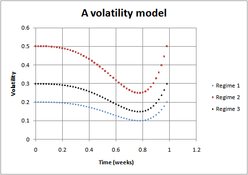
Figure 4.1: Volatility vs. time

Chapter 5 Defaultable bonds

5.1 The Market Model

We consider a market on a probability space $(\Omega,\mathcal{F},P)$, with a finite state space $\chi=\{1,2,\dots,k\}$. The market dynamics are modelled by an age-dependent process $X=\{X_{t}\}_{t\geq 0}$ on $\chi$, as described by equations (2.6) and (2.7). We define the following market parameters as the functions

$$r:\chi\rightarrow(0,\infty),\ \mu:(0,\infty)\times\chi\rightarrow(0,\infty),\ \kappa:(0,\infty)\times\chi\rightarrow\mathbb{R},\ \sigma:(0,\infty)\times\chi\rightarrow(0,\infty).$$ (5.1)

Here, $r,\mu,\kappa,\sigma$ are the interest rate, the drift coefficient, the dividend payout rate and the volatility, respectively.

We consider a structural model of the company’s bond, in which the company defaults on its bond if its asset value drops below a certain threshold. The company’s asset value, $A_{t}$, is assumed to follow a geometric Brownian motion modulated by an age-dependent process $X_{t}$ given by equations (2.6) and (2.7). Thus,

$$dA_{t}=A_{t}\left[\left(\mu(t,X_{t})-\kappa(t,X_{t})\right)\,dt+\sigma(t,X_{t})\,dW_{t}\right],\ A_{0}>0$$ (5.2)

where $\{W_{t}\}_{t\geq 0}$ is a standard Wiener process independent of $X$. The market is also assumed to contain an amount $B_{t}$ a locally risk-free money-market account, where

$$B_{t}=e^{\int_{0}^{t}r(X_{u})\,du}.$$ (5.3)

We use the structural approach to model the credit risk, i.e the risk of the company defaulting on its debt (bonds). We regard the firm’s equity as well as the defaultable bond as contingent claims on the firm’s assets. The equity and the debt of the company are denoted by $E_{t}$ and $D_{t}$, respectively.

5.1.1 Model 1

The first model that we consider is Merton’s classical model ([18]), with a few modifications to account for the fact that the market is modulated by an age-dependent process. We consider a coupon-free bond that can default only on maturity ($t=T$). In the event of a default, the creditors are entitled to the firm’s assets under consideration. Hence, the firm’s equity holders receive a payoff only if $A_{T}>K$, where $K$ is a certain threshold. The total payoff, at maturity, to the equity holders, is

$$E(T,A_{T},X_{T})=(A_{T}-K)^{+}=\max(A_{T}-K,0).$$ (5.4)

The price of the defaultable bond at maturity is given by

$$D(T,A_{T},X_{T})=\min(A_{T},K)=K-(K-A_{T})^{+}.$$ (5.5)

Since the above payoff is the same as that of a portfolio consisting of a default-free loan with face value $K$, maturing at time $T$ and a short European put option on $A_{t}$ with dividend rate $\kappa(t,X_{t})$, strike price $K$ and maturing at time $T$, it suffices to solve the problem of pricing European call options under the same market model. We have done that in 4.3.1. Therefore, we do not produce any further details here.

5.1.2 Model 2

Merton’s classical model does not allow a premature default. It may be that there is a critical threshold below which the firm would be disposed to default on its debt. Such a model is more favourable to the owners of the defaultable bonds. We consider a model where the firm defaults if the asset value $A_{t}$ dips below a critical threshold $J$ for any time $t\in(0,\infty]$, or if the terminal asset value, $A_{T}$ is less than $K$. We assume that $J<K$. Define the following stopping times

$$\tau_{1}=\begin{cases}T,\ \text{if }A_{T}<K\\ \infty,\ \text{otherwise},\end{cases}$$ (5.6)

and $\tau_{2}=\inf\{t\in(0,T]|A_{t}<J\}$. If $A_{t}$ never drops below $J$, we set $\tau_{2}=\infty$. Then the default time, $\tau$, is given by

$$\tau=\min(\tau_{1},\tau_{2}).$$ (5.7)

If the default time is infinity, the firm does not default and the bondholders receive their principal entirely. We can write the value of the defaultable bond at time $T$ as

$$D(T,A_{T},X_{T})=K-(K-A_{T})^{+}+(A_{T}-K)^{+}\mathds{1}(\min_{t\leq T}A_{t}<J).$$ (5.8)

The above payoff can at once be recognised as that of a portfolio consisting of the following three components:

1. A default-free loan of face value $K$, with maturity $T$,

2. A short European put option on $A_{t}$ with dividend rate $\kappa(t,X_{t})$, strike price $K$ and maturing at time $T$, and

3. A long European down-and-out call option with strike price $K$, barrier $J$ and maturing at time $T$.

The value of the defaultable bond under this model is at least as much as that under Merton’s classical model, due to the presence of the third term in (5.8). The bondholders are thus better protected. If the volatility does not depend explicitly on time, i.e. if $\sigma(t,i)=\sigma(i)$ for all $t$ and $i$, then the pricing and hedging problems may be addressed using our analysis in 4.3.2.

5.1.3 Model 3

In this model, the criteria for a default are the same as that for Model 2. The recovery rule, however, is different. In case of a premature default, the bondholders are paid a fraction of the face value of the bond at a pre-determined constant recovery rate, $\delta$, which satisfies the following inequality

$$0\leq\delta\leq\frac{J}{K}\left(\leq 1\right).$$ (5.9)

The procedure for debt recovery is the same as that in Model 2 if the firm defaults at maturity. If the firm does not default, the debt is paid of entirely at maturity. The value of the defaultable bond at maturity can thus be written as

$$D(T,A_{T},X_{T})=\min(A_{T},K)\mathds{1}(\tau\geq T)+\delta KB(\tau,T,X_{\tau})\mathds{1}(\tau<T),$$ (5.10)

where $B(\tau,T,X_{\tau})$ denotes the price at time $\tau$ of a default-free couponless bond with unit face value and maturity $T$. This model is different from the two models previously discussed in that the recovery is at the time of the default, and not necessarily strictly at maturity. As in Model 2, an integral equation formalism can be used in the case where the volatility has no explicit time-dependence.

The market we are considering is incomplete (i.e not all contingent claims can be perfectly hedged by self-financing strategies). This is due to the presence of semi-Markov modulated regime switching. We can, however, minimize the residual risk arising from the incompleteness of the market. We look for the price of derivative securities that minimizes the residual risk. This can be done by considering the Föllmer-Schweizer decomposition of the relevant contingent claim.

References

- [1] Arendt W., Batty C., Hieber, M. and Neubrander, F., Vector-valued Laplace Transforms and Cauchy Problems, Birkhauser 2001.
- [2] Banerjee, Ghosh, Iyer, “Pricing defaultable Bonds in a Markov Modulated Market”, Stochastic Analysis and Applications 30 (2012), 448-475.
- [3] Basak G. K., Ghosh Mrinal K. and Goswami A., Risk minimizing option pricing for a class of exotic options in a Markov-modulated market, Stoch. Ann. App. 29:2(2011), 259-281.
- [4] Buffington J. and Elliott R. J., American options with regime switching, Intl. J. Theor. Appl. Finance 5(2002), 497-514.
- [5] Deshpande A. and Ghosh M. K., Risk minimizing option pricing in a regime switching market, Stoch. Ann. App. 26(2008).
- [6] DiMasi G. B., Kabanov Y. and Runggaldier W. J., Mean-Variance hedging of options on stocks with Markov volatility. Theory Probab. Appl., Vol. 39 (1994), 173-181.
- [7] Elliott R.J., Chan L. and Siu T.K., Option pricing and Esscher transform under regime switching, Annals of Finance 1, 423-432 (2005).
- [8] Föllmer H. and Schweizer, M., Hedging of Contingent Claims under Incomplete Information, Applied Stochastic Analysis, Stochastics Monographs, vol. 5 (1991), 389-414.
- [9] Ghosh M. K. and Goswami A., Risk minimizing option pricing in a semi-Markov modulated market, SIAM J. Control Optim. 48(2009), 1519-1541.
- [10] Ghosh M., Saha S., “Stochastic Processes with Age-Dependent Transition Rates”, Stochastic Analysis and Applications, Taylor & Francis, Vol. 23, No. 5, 2005.
- [11] Goswami A., Patel J., Shevgaonkar P., “A system of degenerate non-local parabolic PDE and application”.
- [12] Guo X. and Zhang Q., Closed form solutions for perpetual American put options with regime switching , SIAM J. Appl. Math 39(2004), 173-181.
- [13] Hunt J. and Devolder P., Semi-Markov regime switching interest rate models and minimal entropy measure, Physica A: Statistical Mechanics and its Applications 390, 15(2011), 3767-3781.
- [14] Ikeda, Watanabe, “Stochastic Differential Equations and Diffusion Processes”, North Holland Mathematical Library, 1981.
- [15] Joberts A. and Rogers L. C. G., Option pricing with Markov-modulated dynamics, SIAM J. Control Optim. 44(2006), 2063-2078.
- [16] Kallianpur Gopinath and Karandikar Rajeeva L., Introduction to Option Pricing Theory, Birkhäuser Boston, 2000.
- [17] Mamon R. S. and Rodrigo M. R., Explicit solutions to European options in a regime switching economy, Operations Research Letters 33(2005), 581-586.
- [18] Merton, R. C. 1974. On the Pricing of Corporate Debt: The Risk Structure of Interest Rates. Journal of Finance. 29:449-470
- [19] Nunn W. R., Desiderio A. M., “Semi-Markov Processes: An Introduction”, Centre for Naval Analyses, CRC 335, July 1977.
- [20] Pazy A., Semigroups of Linear Operators and Applications to Partial Differential Equations, Springer-Verlag, 1983.
- [21] Pham H., Rheinländer T. and Schweizer, M., Mean-variance hedging for continuous processes: new proofs and examples, Finance Stoch.(1998) 173-198.
- [22] Pyke R., Markov renewal processes: definitions and preliminary properties, Ann. Math. Statist. Vol. 32 (1961), pg. 1231–1242.
- [23] Pyke R., Markov renewal processes with finitely many states, Ann. Math. Statist. Vol. 32 (1961), pg. 1243–1259.
- [24] Schweizer M., A Guided Tour through Quadratic Hedging Approaches, E. Jouini, J. Cvitanić, M. Musiela (eds.), Option Priing Interest Rates and Risk Management, Cambridge University Press (2001), 538-574.
- [25] Shiryaev A.N., Essentials of Stochastic Finance: Facts, Models, Theory, 1999.
- [26] Shreve S. E., Stochastic Calculus for Finance-II: Continuous-Time Models, Springer, 113-115.