Transverse velocity shifts in protostellar jets: rotation or velocity asymmetries?

Abstract

Observations of several protostellar jets show systematic differences in radial velocity transverse to the jet propagation direction, which have been interpreted as evidence of rotation in the jets. In this paper we discuss the origin of these velocity shifts, and show that they could be originated by rotation in the flow, or by side to side asymmetries in the shock velocity, which could be due to asymmetries in the jet ejection velocity/density or in the ambient medium. For typical poloidal jet velocities ($\sim 100-200$ km s^-1), an asymmetry $\gtrsim$ 10% can produce velocity shifts comparable to those observed. We also present three dimensional numerical simulations of rotating, precessing and asymmetric jets, and show that, even though for a given jet there is a clear degeneracy between these effects, a statistical analysis of jets with different inclination angles can help to distinguish between the alternative origins of transverse velocity shifts. Our analysis indicate that side to side velocities asymmetries could represent an important contribution to transverse velocity shifts, being the most important contributor for large jet inclination angles (with respect the the plane of the sky), and can not be neglected when interpreting the observations.

1. Introduction

Astrophysical jets can be found in a variety of physical scales, energies and environments. For instance, planetary nebulae, cataclysmic variables, neutron stars and supernovae sometimes show bipolar jets (e.g., Livio, 1999). In active galactic nuclei, we can see accretion powered jets emanating from the central engine (Yuan & Narayan, 2014). In star forming regions, jets are ubiquitous and can be found associated with young stellar objects ranging from brown dwarfs to high mass stars (e.g., Li et al., 2014).

Star forming regions like Orion and Taurus show a wealth of protostellar jets. For more than sixty years they have been studied observationally, theoretically and, more recently, numerically. These different approaches allowed to conclude that protostellar jets are also accretion powered collimated outflows, ejected episodically from the inner part of the accretion disks with the help of a magnetic field. Supersonic variations in the ejection velocity produce Herbig-Haro (HH) objects as emitting post-shock cooling regions (e.g., Reipurth & Bally, 2001).

Some of the HH objects have a knotty structure, while other have a bow-shaped form. It is still a matter of debate whether there is a contribution of a collimated stellar wind component, or a broad, non-collimated disk wind component, and if the ejections are periodic or not. Also, jets launched from the accretion disks are believed to rotate (e.g., Ferreira et al., 2006). If measured, the rotation of the jet with respect to its axis would give an estimation of the amount of angular momentum extracted from the star-disk system. This is a key parameter that can be used to understand the origin of protostellar jets, and might also help to understand the general mechanism responsible for the production of astrophysical jets at different scales.

Recent observations of HH jets show transverse velocity shifts in several emission lines. Davis et al. (2000) first observed a shift in the H₂ lines for the molecular jet HH 212. Bacciotti et al. (2002) observed the DG Tau micro-jet, much closer to the central source and in atomic lines, finding a similar shift in several emission lines. Other authors observed later a larger sample of objects getting similar results: Woitas et al (2005), Coffey et al. (2004, 2007, 2012) for class II objects, Chrysostomou et al. (2008) for Class I objects and Lee et al. (2007, 2008); Choi et al. (2011); Coffey et al. (2011) for class 0 (or 0/I) objects.

From these results, important consequences on the jet ejection mechanism have been inferred. Different models predict that jets are ejected from different regions of the disk. For instance, in the “X-wind” scenario the jet is ejected from the region of interaction between the protostar’s magnetosphere and the disk (Shu et al., 2000), while in the “disk-wind scenario”, the jet is magnetocentrifugally ejected from an extended portion of the disk surface (Blandford & Payne, 1982).

If interpreted as rotation, observations imply a range of ejection radii around $\sim 1$ AU (e.g. Ferreira et al. 2006), therefore excluding the X-wind as possible mechanism for the jet ejection, and favoring the disk-wind scenario. On the other side, recently Lee et al. (2008) determined wind launching radii $\lesssim 0.05-0.30$ AU, consistent with the X-wind model (Shu et al., 2000).

In agreement with the rotation interpretation of the data, jet and counter-jet rotate in the same sense in the Th 28 and RW Aur jets. In both cases, nevertheless, the sense of rotation observed in the disk and the jet are opposite (Cabrit et al., 2006; Louvet et al., 2016). In other cases the observations did not detect any rotation given the limits of resolution of the observations (HH 30 in Pety et al. 2006 and Coffey et al. 2007, HH 212 in Codella et al. 2004, RY Tau in Coffey et al. 2015). Puzzling, recent near-UV observations (Coffey et al., 2012) of the RW Aur jet showed velocity shifts which, if interpreted as rotation, give a sense of rotation consistent with that of the disk (but opposite with respect to previous optical observations), which were not detectable anymore in following-up near-UV observations six months later at levels above the limiting resolution of the observations (Coffey et al., 2012).

While most of the studies have interpreted the presence of velocity shifts as due to the rotation of the jet material, a few works have studied alternative mechanisms. Cerqueira et al. (2006, hereafter CER06), using numerical simulations, showed that jet precession may lead to velocity shifts similar to those observed, while Soker (2005) proposed disk asymmetries as a possible alternative mechanism. Among the observed T Tau jets with velocity shifts, DG Tau has observed precession (Dougados et al., 2000; Lavalley-Fouquet et al., 2000) and the model developed by CER06 may be applied to this jet. Launhardt et al. (2009) have also inferred, through radio observations, that the molecular outflow associated with a T-Tauri star in the CB 26 Bok globule (in Taurus-Aurigae) is rotating. They have suggested that the outflow is also precessing. For these cases, it seems plausible that the effects of precession should be carefully taken into account when considering radial velocity shifts as a fiducial evaluation for jet rotation.

More recently, Pech et al. (2012) investigated the origin of the radial velocity shift (of the order of 2 km s^-1) observed in the HH 797 outflow. In order to explain the observed data, they have considered both precession and rotation, concluding that rotation may probably account for the shifts. It seems at a first glance, however, that the HH 797 jet is precessing, as it is suggested by the wiggling of the outflow far from the driving source (see Figure 1 in Pech et al., 2012).

In this paper we critically analyze the key hypothesis done implicitly when interpreting the observed velocity shifts as rotation: the absence of side to side (i.e., with respect to the jet axis) velocity asymmetries. In particular, we will show analytically (Section 2) and by numerical models (Section 3) that the presence of velocity asymmetries may generate effects resembling those observed, i.e., that there is a degeneracy between toroidal and asymmetric poloidal velocities, which can be disentangled only by a statistical analysis of a large sample of HH jets. In Section 4 we discuss the results, and in Section 5 we draw our conclusion.

2. The origin of transverse velocity shifts in HH jets

Observations of transverse velocity shifts (TVS) are commonly interpreted as evidence of jet rotation. This is valid as long as the dominant component in the radial velocity is the rotation velocity. All the previous observational efforts done in order to estimate the TVS are based on the assumption that the jet velocity is symmetric across the jet radius, and that the TVS are only due to the presence of a given rotational profile. Nevertheless, the poloidal jet velocity, which can have a large variability even for a given jet (Ferreira et al., 2006), is a key point to infer (from the observational point of view; see, for instance, Bacciotti et al., 2002) the region at the surface of the accretion disk where the outflow is actually produced/launched.

A Herbig-Haro jet has a typical poloidal velocity of 100-200 km s^-1 (Reipurth & Bally, 2001). The presence of a side to side (with respect to the jet axis) gradient in the jet velocity (hereafter, a “velocity asymmetry”) can also contribute to the observed TVS. To better illustrate this point, in this section we will compute synthetic position-velocity diagrams and, analyzing them similarly to how is done by observers, we will demonstrate that rotation and velocity asymmetries produce similar TVS. Then, we will show how it is possible to understand the origin of TVS by a statistical analysis of the existing data.

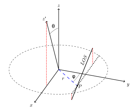
Figure 1.— Schematic representation of the jet geometry. The plane of the sky is represented by the $y,z^{\prime}$ plane. The jet moves along the $z$-axis, with an inclination angle $\theta$ with respect to the plane of the sky. The direction of the line of sight (LOS) is parallel to the planes $xz$, $xz^{\prime}$ and forms an angle $\theta$ with the $xy$ plane.

We consider a jet moving along the $z$-axis with velocity $v_{z}$ and rotating around the $z$-axis with velocity $v_{\phi}$ (see figure 1). Assuming for simplicity that the jet physical parameters (i.e., jet density, temperature, velocity and chemical composition) are independent of $z$, the radial velocity $v_{r}$ (along the line of sight) of a fluid element $P$ is given by

$$v_{r}(y,\phi)=v_{\phi}(r)\cos\phi\cos\theta+v_{z}(r,y,\phi)\sin\theta\;,$$ (1)

where $\theta$ is the inclination angle of the jet with respect to the plane of the sky, $\phi$ is the angle between the segment connecting $P$ with the jet axis and the $y$-axis, $r$ is the distance from $P$ to the jet axis, and $y=r\cos\phi$ (see figure 1).

The emission line intensity per unit velocity $I(y,v)$, observed at a certain distance $y$ from the jet axis, can be computed by integrating the emission coefficient per unit velocity $i(r,v)$ along the line of sight, i.e. by solving the “Abel transform”:

$$I(y,v)=\int_{y}^{\infty}\frac{i(r,v)r}{\sqrt{r^{2}-y^{2}}}dr\;.$$ (2)

We assume that the emission coefficient per unit velocity $i(r,v)$ is related to the emission coefficient $i(r)$ by

$$i(r,v)=i(r)\;e^{-\frac{(v-v_{r})^{2}}{\sigma^{2}}}\;,$$ (3)

where $\sigma^{2}=\sigma^{2}_{\rm flow}+\sigma^{2}_{\rm instr}$ is the sum of the flow and the instrumental velocity dispersion. Typically $\sigma^{2}_{\rm instr}\gg\sigma^{2}_{\rm flow}$, as e.g. $\sigma^{2}_{\rm instr}\approx 50$ km s^-1 for the “Space Telescope Imaging Spectrograph” (STIS) on the Hubble Space Telescope (HST). Therefore, we can assume $\sigma^{2}\approx\sigma^{2}_{\rm instr}$.

By using equations 1 and 3, equation 2 reduces to

$$I(y,v)=\int_{y}^{R}\frac{i(r)e^{-(v-v_{\phi}y/r\cos\theta-v_{z}\sin\theta)^{2}/\sigma^{2}}r}{\sqrt{r^{2}-y^{2}}}dr\;.$$ (4)

We assume a Gaussian dependence for the emissivity $i(r)\propto\exp(-r/r_{0})^{2}$ and a keplerian rotation velocity $v_{\phi}=v_{\phi,0}(r/r_{0})^{-1/2}$ (with $v_{\phi}=v_{\phi,0}(r/r_{0})$ for $r<r_{0}$ to avoid an infinity at $r=0$). The jet velocity $v_{z}$ is in general a complicated function of $r,y,\phi$, e.g. a decreasing function of $r$ and/or asymmetric with respect to $y$ and $\phi$. To focus only on the effects of asymmetries with respect to the main axis of the jet (projected in the plane of the sky) we take a simple jet velocity given by a modified “top-hat” profile, i.e. $v_{z}=v_{z,0}(1-\Delta v_{z,0}x/R_{j})$, being $R_{j}=1$ the jet radius. Other velocity and intensity profiles will give similar (at least qualitatively) results.

We use equation 4 to compute synthetic position-velocity (PV) diagrams. From the PV diagrams we extract intensity profiles at positions symmetric with respect to the jet axis. A systematic gradient in the transverse Doppler profile is what is usually interpreted as rotation in the observations.

Figure 2 shows intensity profiles at $y=\pm\,0.5\,R_{j}$, for a rotating jet with $v_{\phi,0}=200$ km s^-1, $r_{0}=0.001$ (corresponding to $v_{\phi}=9$ km s^-1 at $r=0.5\,R_{j}$, consistent with the toroidal velocity estimated by Coffey et al. 2007), $\Delta v_{z,0}=0$ (left panels), and for a jet with side to side velocity asymmetries with $\Delta v_{z,0}=0.1$, $v_{\phi,0}=0$ (right panels). The poloidal jet velocity is equal to $v_{z_{0}}=200$ km s^-1 in both cases.

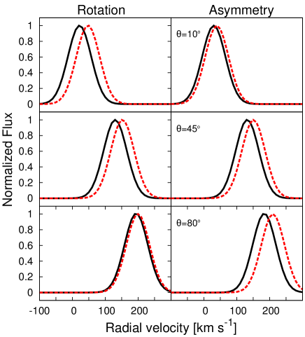
Figure 2.— Intensity profiles of synthetic emission lines computed in positions symmetric with respect to the jet axis (black, full line and red, dashed lines), for a jet with rotation (left panels) and with velocity asymmetries (right), for inclination angles $\theta=10^{\circ},45^{\circ},80^{\circ}$ (upper, middle, lower panels respectively) with respect to the plane of the sky. The radial velocity differences, given by the shifts in the synthetic emission lines, depend strongly on the jet inclination angle. In particular, rotation (asymmetry) produces a larger velocity shift for small (large) jet inclination angles.

Figure 2 shows that unless the jet inclination angle is $\theta\approx 0^{\circ}$ or $\theta\approx 90^{\circ}$, rotation and velocity asymmetries both contribute to the radial velocity shift. Therefore, observations of radial velocity shifts in a jet do not allow to determine with precision the amount of rotation and velocity asymmetry present in the jet, unless the jet is moving nearly in the plane of the sky.

Figure 2 also shows that the TVS produced by rotation and velocity asymmetry strongly depend on the jet inclination angle. In fact, the velocity gradient between two fluid elements located at positions symmetric with respect to the jet axis (i.e. at $\phi=0$, $y=y_{0}$ and $y=-y_{0}$) is given (see equation 1) by:

$$\Delta v_{r} = v_{r}(y_{0},0)-v_{r}(-y_{0},0)=$$ (5)

$$= 2v_{\phi}(r_{0})\cos\theta+\Delta v_{z}\sin\theta$$

where $\Delta v_{z}=v_{z}(y_{0},0)-v_{z}(-y_{0},0)$ is the transverse gradient of the jet velocity.

If the jet is nearly axisymmetric, $\Delta v_{z}\ll v_{\phi}$. In this case $\Delta v_{r}\sim 2v_{\phi}\cos\theta$, and $\Delta v_{r}$ decreases for larger jet inclination angles. If, on the other side, the transverse velocity shift is mainly due to side to side asymmetries in the poloidal component of the jet velocity ($\Delta v_{z}\gg v_{\phi}$), $\Delta v_{r}\sim\Delta v_{z}\sin\theta$ and $\Delta v_{r}$ increases with the inclination angle of the jet.

In general we do not know a priori which velocity component dominates the radial velocity, but we can estimate the relative importance of $v_{\phi}$ vs. $\Delta v_{z}$ by considering jets at different inclination angles, as rotation (if present) will dominate the observed velocity shifts at small inclination angles (i.e., $\Delta v_{r}\propto v_{\phi}$ if $\theta\ll\Delta v_{z}/v_{\phi}$, see equation 5), and velocity asymmetries (if present) will dominate the velocity shifts at large inclination angles (i.e., $\Delta v_{r}\propto\Delta v_{z}$ if $\theta\gg v_{\phi}/\Delta v_{z}$).

Let us consider existing data of TVS determined observationally for atomic lines. The observations were presented by Coffey et al. (2004) and Coffey et al. (2007) and include the CW Tau, DG Tau, HH 30, RW Aur and TH 28 protostellar jets, observed by STIS on the Hubble Space Telescope The HH 30, CW Tau, DG Tau are located in the Taurus molecular cloud at a distance of 140 pc, while Th 28 and RW Aur are located in Lupus 3 (140 pc) and Auriga (170 pc) respectively. The estimated inclination angles are (see Coffey et al. 2004, 2007 and references therein) 1^∘ (HH 30), 10^∘ (Th 28), 41^∘ (CW Tau), 44^∘ (RW Aur), 52^∘ (DG Tau).

To estimate the relative importance of $v_{\phi}$ and $\Delta v_{z}$, we computed, for each jet (see Table 1), the averages of the transverse velocity shifts measured at different distances from the jet axis by Coffey et al. (2004, Table 3) and Coffey et al. (2007, Table 3) for the [O I]$\lambda 6300$, [N II]$\lambda 6583$, [S II]$\lambda 6716$, and [S II]$\lambda 6731$ emission lines. Other emission lines presented by Coffey et al. (2004, 2007) are not included as they are observed in a more limited number of jets.

	$\Delta v_{r}$ for	$\Delta v_{r}$ for	$\Delta v_{r}$ for	$\Delta v_{r}$ for
Jet	[O I]$\lambda$6300	[N II]$\lambda$6583	[S II]$\lambda$6716	[S II]$\lambda$6731
	(km s-1)	(km s-1)	(km s-1)	(km s-1)
HH 30 blue	3.75	1.5	-1.67	-2.4
TH 28 red	13.4	16.5	3	1.2
TH 28 blue	11.5	6.67	…	…
CW Tau blue	14	13.5	…	-2
RW Aur red	15.25	14	-1.5	-1.33
DG Tau blue	17.6	6.67	2.33	2.6

Table 1Observed transverse velocity shifts

In Figure 3 we show the transverse velocity shift $\Delta v_{r}$ as a function of the jet inclination angle for these protostellar jets and the [O I] and [N II] emission lines. The other two lines considered do not show any measurable TVS (see Table 1). For each emission line, we fit the data by using equation 5. To estimate the accuracy of the fit we have computed the parameter $Q$, which is the probability that, given the fit to the data, data with Gaussian noise (assumed here to be 5 km s^-1) have a $\chi^{2}$ larger than the one determined in the fit. Values of $Q\lesssim 1$ indicates an acceptable fit, while smaller values (Q $\approx 0$) indicate that the fit is poor.

The results are the following: for a purely rotating jet, $\Delta v_{r}=2v_{\phi}\cos\theta$, with $v_{\phi}=6.9\pm 1.6$ km s^-1, $Q=0.1$ for the [O I] line, and $v_{\phi}=5.5\pm 1.5$ km s^-1, $Q=0.15$ for the [N II] line. For a jet with velocity asymmetry we get $\Delta v_{r}=\Delta v_{z}\sin\theta$ with $\Delta v_{z}=23.8\pm 4.4$ km s^-1, $Q=0.28$ for the [O I] line, and $\Delta v_{z}=17.5\pm 5.6$ km s^-1, $Q=0.07$ for the [N II] line. The best fit is obtained by including both rotation and velocity asymmetries, with $v_{\phi}=3.7\pm 1.0$ km s^-1, $\Delta v_{z}=15.4\pm 3.2$ km s^-1, $Q=0.8$ for the [O I] line, and $v_{\phi}=3.6\pm 1.9$ km s^-1, $\Delta v_{z}=9.1\pm 6.4$ km s^-1, $Q=0.25$ for the [N II] line.

Fits to the data give typical velocities $v_{\phi}\sim 5$ km s^-1 and $\Delta v_{z}\sim 15$ km s^-1. Although this result should be taken carefully because of the low statistics and the approximations used (e.g., we are assuming that $v_{\phi}$ and $\Delta v_{z}$ are the same for all jets, and this is not necessarily true), it seems to indicate that velocity asymmetries are an important component of the velocity shifts, dominant for jets with “large” inclination angles ($\theta\gtrsim\arctan(2v_{\phi}/\Delta v_{z})$, see equation 5).

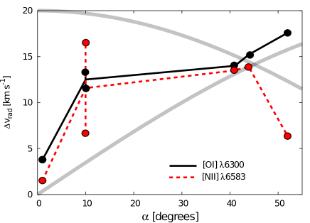
Figure 3.— Comparison of observed shift in the transverse velocity with two simple model represented by $\sin\theta$ and $\cos\theta$ curves for the velocity asymmetry and rotation cases. The data points are from Coffey et al. (2004) and Coffey et al. (2007) and correspond (from left to right) to HH 30 (1^∘), Th 28 (10^∘), CW Tau (41^∘), RW Tau (44^∘), DG Tau (52^∘).

3. Numerical simulations

When the jet inclination is considered, different shock regions, located at different positions $z$ along the direction of propagation of the jet, contribute to the radial velocity. In this Section, we will use three dimensional numerical simulations of protostellar jets to take in account multi-dimensional effects neglected in Section 2.

We have used the Yguazú-a code to simulate jets in three-dimensions. The Yguazú-a is an adaptive grid code that uses a flux vector splitting scheme (see van Albada, van Leer & Roberts, 1982) to evolve the equations of hydrodynamics. At each time step, the code integrates a system of rate equations for 17 atomic/ionic species, namely: H I, H II, He I, He II, He III, C II, C III, C IV, N I, N II, N III, O I, O II, O III, O IV, S II, S III. A non-equilibrium cooling function is then calculated. The detailed reaction equations as well as the cooling function are given in Raga, Navarro-González & Villagrán-Muniz (2000); Raga et al. (2007).

The number of cells in the computational box is ($x$, $y$, $z$) = (128, 128, 512). Each cell has a physical dimension of 8.59$\times 10^{13}$ cm, or 5.7 AU, for all the three dimensions (in a Cartesian coordinate system). A jet with a radius of $R_{j}=37.4$ AU is injected from the $xy$ plane at $z=0$ (see Figure 1), and propagates in the positive $z$ direction. The jet to ambient medium density ratio is given initially by $n=n_{j}/n_{a}=10$, where $n_{j}=1\,000$ cm^-3. The initial jet ionization fraction of H is 0.1. The jet temperature is $T_{j}=10^{4}$ K, and the ambient medium temperature is $T_{a}=10^{3}$ K. The initial setup is equivalent to the one employed in CER06.

We present here the results from four different numerical simulations, differing for the presence (or not) of rotation, precession and side to side velocity asymmetry (see Table 2). The baseline jet velocity (in the $z$ direction) is the same for all the models: 300 km s^-1. Model M1 does not have rotation while the others do have. The model M4 has also a precession (see below). All models have a sinusoidally variable jet velocity (along the $z$ direction):

$$V_{j}\equiv V_{z}=V_{0}\cdot\bigg{[}1+A\,{\rm sin}\bigg{(}\frac{2\pi}{P}t\bigg{)}\bigg{]}\cdot[1+f(y)]$$ (6)

where $V_{0}=300$ km s^-1, $A=0.33$ and $P=8$ yr (these parameters are chosen to reproduce the velocity structure of the DG Tau micro-jet; Dougados et al. 2000; Raga et al. 2001). Models M2, M3 and M4 have $f(y)=0$. This is the typical top-hat profile for the $V_{z}$ adopted in several numerical studies of jets. The model M1 has $f(y)=0.025\;{\rm sign}(y)$, where ${\rm sign}(y)$ is a function that returns the sign of the $y$ coordinate in the computational domain. This implies that at any time step $\Delta V_{z}(t)=0.05\;V_{j}(t)$ in the $yz$ plane. We could expect, then, a maximum side to side jet asymmetry of $\Delta V_{z}=20$ km s^-1. We are artificially introducing an asymmetry between both sides of the jet axis in the jet velocity, without arguing about its nature. Although quite speculative, this model will serve to illustrate what can actually occur if a jet has, for some reason, a side to side asymmetry in shock velocities.

Model	$\tau_{\rm prec}$	$V_{\phi}\times(r/R_{j})$	$\Delta V_{z}$
	(years)	(km s-1)	(km s-1)
M1	0	0	$\leq$ 20
M2	0	$\lesssim$ 10	0
M3	0	8	0
M4	8	8	0

Table 2The simulated models

M2, M3 and M4 are rotating jet models with different rotational velocity profiles ($V_{\phi}=\sqrt{V_{x}^{2}+V_{y}^{2}}$). In model M2 $v_{\phi}$ is given by:

$$V_{\phi}=\frac{V_{j}}{40}$$ (7)

so the rotational velocity will fluctuate in time with values ranging from 5 and 10 km s^-1 (it is constant through the jet cross section). The model M3 is the same model that we have presented in CER06. For this case:

$$V_{\phi}=8~{}{\rm km~{}s}^{-1}\cdot\frac{R_{j}}{r}$$ (8)

where $r=\sqrt{x^{2}+y^{2}}$. As in CER06, profile has been truncated at $R=0.15R_{j}$. The toroidal velocity ranges then from $V_{\phi}=55$ km s^-1 to 8 km s^-1 at the jet radius (see also Cerqueira & de Gouveia Dal Pino, 2004). The model M4 is similar to M3, but the jet is actually precessing with a half opening angle of 5^∘ and with a precessional period of $\tau_{\rm prec}=8$ years.

The strategy that we have used here in order to build the synthetic slits, the synthetic line profiles and to analyze the line profile in terms of its components (low-, medium- and high-velocity component) is the same that we have presented in CER06. Firstly, we calculate the emission coefficients for the [O I] and [S II] emission lines (Raga et al., 2004). To build velocity channel maps (VCM) for a given radial velocity $V_{r}$, the local emissivity is smeared out (in radial velocity, or wavelength) using a Gaussian profile. The broadening of the line profile is estimated using the characteristic sampling (we use $\Delta V_{r}=10$ km s^-1) of our VCMs and the local sound speed, $c_{s}$. We then define the local dispersion of the line profile as $\sigma=\sqrt{\Delta V_{r}^{2}+c_{s}^{2}}$.

To build the line profiles we need to define an artificial slit, which depends on the position in the VCMs, and we need to project our computational box on the plane of the sky. The radial velocity is then the projection of the velocity at a given cell along the line of sight, which can make an arbitrary angle with the $x-$axis. Increasing the inclinations angles will shift the profiles to increasingly negative radial velocities.

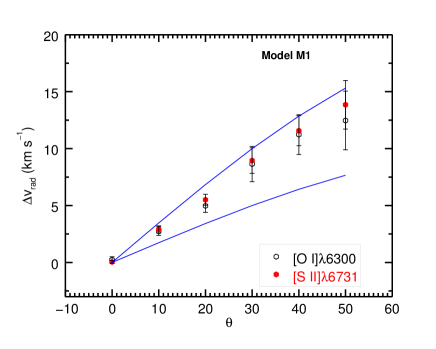
Figure 4.— Radial velocity estimates from different line profiles (filled circles, [S II]6731; open circles, [O I]6300), and for different inclination angles from 0^∘ to $50^{\circ}$, for the model M1 (i.e., the model with side to side shock velocity asymmetries). For each inclination angle, we have used four different regions along the jet, and six different positions across the jet axis to compute $\Delta v_{\rm rad}$. The dispersion in the radial velocity around its mean value is indicated by the error bars for each inclination angle. The solid curves are sine functions with amplitude of 10 and 20 km s^-1.

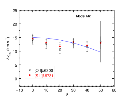
Figure 5.— The same as in Figure 4, but for M2 model (with a jet rotation velocity constant through the jet cross-section). Here, the solid curve is a cosine function with amplitude of 15 km s^-1.

In all models the VCMs were built first for the raw data and then convolved with a profile in order to mimics the instrumental effect on the data. For the convolution procedure we have assumed a Gaussian profile, that goes to zero at 3 pixels of distance from a given point in the map. At the distance of DG Tau, for instance, this corresponds to a point-spread function of $0.1$ arcsec (of FWHM).

The spectra extraction procedure has been already presented in CER06 and is described in detail in the Appendix. Briefly, we define four different regions along the jet axis, and near the jet inlet. These regions have a superposition of one cell along the jet propagation direction. For each one of these regions, we define a $3\times 3$ square region for which a mean spectra is taken (i.e., we sum up nine spectra to increase the signal). To build up the line profile, we use VCM from -400 km s^-1 to 100 km s^-1, with a 10 km s^-1 sampling. We did the same procedure for different inclination angles, namely, 0, 10, 20, 30, 40 and 50 degrees. The convolution procedure and the differences in the inclination angles, as well as the presentation of new models (M1 and M2) is the main difference of these results when compared with those presented in CER06.

In Figure 4 we show the radial velocity shift for model M1, taking into account the [S II] and [O I] emission lines. The dispersion around the mean value is also plotted as vertical, error bars. The results for the non-rotating M1 model in Figure 4 is compared with the functions $20\,\sin\theta$ and $10\,\sin\theta$. They are consistent with a sinusoidal fit, with different amplitudes for the different emission lines.

In Figure 5 we show the same result for the (rotating) M2 model. Now the data are compared with the function $15\cos\theta$. They are consistent with a cosine trend, although slightly below it (for the chosen value of 15 km s^-1 for the amplitude of the oscillation) except at large jet inclination angles. The same behavior is also seen for the M3 model (see Figure 6). A comparison between figure 5 and figure 6 also shows that the result is nearly independent (at least qualitatively) from the particular dependence of the rotation velocity with radius considered. In Figure 7 we show the difference in the radial velocity for the M4 (rotating and precessing model) as a function of the inclination angle. Depicted also in this figure is the cosine function (for the sake of comparison). Figures 5-7 all show an appreciable TVS. These results are in agreement with those presented by CER06, since their M2 and M4 models are the same as the ones in the present paper. Although less evident, we should note that Smith & Rosen (2007) have also found some TVS in their precession model of molecular jet (see their Figure 14, Regions III and IV). Furthermore, the rotating models discussed in Smith & Rosen (2007) and CER06 display signatures for rotation in the TVS analysis that are not precisely equivalent. In this case, however, the initial rotational profile seems to be at the origin of the differences reported, as has been pointed out by Smith & Rosen (2007), and the results obtained by both are consistent with the expected ones taken into account their adopted initial rotational profiles.

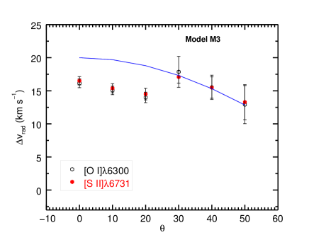
Figure 6.— The same as in Figure 4, but for M3 model (with a jet rotation velocity decreasing as $v_{\phi}\propto r^{-1}$). The solid curve is a cosine function with amplitude of 20 km s^-1.

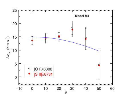
Figure 7.— The same as in Figure 4, but for M4 model (rotating, precessing jet model). The solid curve is a cosine function with amplitude of 15 km s^-1.

4. Discussion

In this paper, we analyze the origin of velocity shifts observed in protostellar jets. Three-dimensional numerical simulations presented in section 3 confirm the results of section 2: radial velocity shifts strongly depend on the jet inclination angle and scale with respect to rotation as $\sim\cos\theta$ and side to side velocity asymmetries as $\sim\sin\theta$.

An interesting difference between the results of the numerical simulations and the observations is the behavior of the velocity shifts for different emission lines. While in the simulations the [O I]$\lambda$6300 and the [S II]$\lambda$6731 emission lines have a similar behavior, in the observations by Coffey et al. (2004, 2007) the [O I]$\lambda$6300 line exhibits velocity shifts much larger than those observed in the [S II]$\lambda$6731 emission line (but these two lines follow a similar behavior in the radial shifts measured by Bacciotti et al. 2002 for the DG Tau micro-jet).

Emission line intensities strongly depend on the jet density profile. The setup of our simulations considers the same abundance for a given atom (with respect to hydrogen) at the jet inlet. In addition, in the simulations presented in this paper we have followed the “standard” recipe of injecting a jet with a top-hat density profile while a “real” jet has a density profile larger on the jet axis (see, e.g., the electron density profile of the HH 30 jet reconstructed by tomographic techniques by De Colle et al. 2010). Therefore, the adopted top-hat velocity and density profiles can actually affect a direct comparison with the observations.

One could think that the results presented in Section 2 depend strongly on the HH 30 data which, moving nearly in the plane of the sky and with very low values of $\Delta v_{r}$, favor a model with low rotation and large velocity asymmetry. This is actually not the case, as the results are not strongly dependent on the HH 30 data. In fact, a fit computed without including the HH 30 emission lines gives $v_{\phi}=5.1\pm 0.7$ km s^-1, $\Delta v_{z}=12.2\pm 2.1$ km s^-1, and $Q=0.96$ for the [O I] line, and $v_{\phi}=5.8\pm 2.2$ km s^-1, $\Delta v_{z}=4.2\pm 6.3$ km s^-1, and $Q=0.40$ for the [N II] line, then confirming that velocity asymmetries are an important component of the radial velocity shifts, at least at large jet inclination angles.

As a consequence, jets with low inclination angles should be preferentially used to properly infer the amount of rotation occurring in the velocity shifts. Among the jets considered here, HH 30 is nearly in the plane of the sky but, as mentioned above, does not show radial velocity shifts larger than the statistical error. Th 28 has a small inclination angle ($\theta\sim 10^{\circ}$) with respect to the plane of the sky, and presents large velocity shifts.

As discussed in section 2, if a side to side spatial asymmetry is present in an emission line profile, it becomes very important to address the effect of the asymmetry (possibly due to an asymmetric shock) on the interpretation of the velocity shift as due to rotation.

In general large scale stellar jets are very asymmetric and irregular, while small scale jets exhibit some degree of symmetry. Several jets among those used to measure rotation in jets show asymmetries in the physical parameters. Coffey et al. (2008), using data from STIS, determined the physical parameters (electron and hydrogen density, temperature, and ionization fraction) from PV diagrams in the red-shifted RW Tau and Th 28 jets, and in the blue-shifted DG Tau, HH 30 and CW Tau jets. Among these jets, Th 28, which, as mentioned above, is the most promising jet to infer rotation from radial velocity shift, presents a very clear side to side asymmetry in the electron density, while temperature and ionization fraction are nearly symmetric. The DG Tau jet presents also a strong asymmetry in the electron density, while HH 30 and RW Aur are nearly symmetric (at least, at the position where the slit is located and with the resolution of STIS). For the Th 28 and DG Tau jets, the more obvious explanation for the origin of the asymmetry in the electron and total density is the existence of an asymmetry in the jet velocity.

Several processes, which can create asymmetries in the jet, have been extensively studied, mainly theoretically. They can be of “internal” origin, i.e. due to a non-symmetric injection velocity from the star disk system (e.g., Soker, 2005) or of “external” origin, i.e. due to the jet environment, originated for instance by hydrodynamics of magnetohydrodynamics instabilities (e.g., “kink” modes), by lateral gradients in the density of a stratified interstellar medium (e.g., Canto & Raga, 1996), the presence of photoionization (Bally et al., 2006; Masciadri & Raga, 2001a), a wind on one side of the jet (e.g., Canto & Raga, 1995; Masciadri & Raga, 2001b; Ciardi et al., 2008), or, in general, the motion of the source with respect to the environment. For example, the HH 30 jet shows a small bending from distances of order of 400 AU from the central source (Anglada et al., 2007). As the effect needed to explain the observed velocity shift is quite small ($\sim 10$% of the observed poloidal jet velocity), the required amount of asymmetry is often smaller than the one discussed in the cited papers.

Several authors (e.g., Anderson et al., 2003; Ferreira et al., 2006; Pesenti et al., 2004) have considered, from the observation of transverse shifts, the implications on the jet ejection models, showing that the observation are consistent with the disk-wind ejection mode. Our results imply that jet rotation, if present, is probably smaller than the values inferred by previous authors. That does not imply necessarily that the rotation at the base of the jet is small. Shocks, jet expansion, entrainment, can all potentially lead to a “loss of memory” of the material with respect to the original rotation, as discussed for instance by Fendt (2011) for magnetohydrodynamics shocks in a helical magnetic field. Recent numerical simulations (Staff et al., 2015) showed that the signature of rotation in the jet can be even non-Keplerian, which means that the signature showed by RW Aur, in which the jet seems to rotate in the sense contrary to the disk rotation can, in fact, occur. This pose an additional difficulty, in our view, to interpret side to side differences in radial velocity as rotation, since we need to trace back the phase of the torsional Alfvèn wave that is actually producing the outflow at a given point in the jet.

Observations of molecular jets in some cases also show small velocity shifts ($\lesssim$ a few km s^-1) which can be interpreted as jet rotation. Although in this paper we have limited our analysis to atomic jets, our conclusions are also applicable to molecular jets, where the rotation features are observed at larger distances from the disk-star system (both along and across the jet axis), i.e. at the “edge” of the jet, where the interaction with the environment is expected to be more important. Zapata et al. (2015) have recently suggested that observed TVS could be originated by rotation of the entrained material.

5. Conclusion

In this paper, we have discussed the uncertainties present when interpreting as rotation the velocity shifts observed in atomic protostellar jets. We have shown that asymmetric shocks, possibly produced as the results of the interaction with the environment or by asymmetries in the ejection velocity from the disk-star system, may produce effects similar to those produced by rotation. We have also quantified, analytically and by detailed numerical simulations, how in jets with large inclination angles transverse velocity shifts may be dominated by jet asymmetries, while rotation, if present, should dominate in jets with low inclination angles.

The main uncertainties in this study reside in the low statistics existing in our analysis (only six jets) and on the fact that we are assuming that rotation and velocity asymmetry are the same for all jets. The analysis presented here does not pretend to be complete, as other factors (e.g., the agreement between the sense of rotation of jet and disk, the poloidal extension of the region showing velocity shifts) should be considered when analyzing the observed TVS. Nevertheless, by analyzing existing data of a limited sample of atomic protostellar jets, we have clearly shown that velocity asymmetries (whatever is their origin) seem to play a very important role in determining the amount of transverse velocity shift present in protostellar jets.

Our results imply that only a detailed modeling of the observations, which include all the effects that can potentially play a role in generating velocity shift, combined possibly with numerical simulations or with novel analysis of the data (e.g., the principal component analysis suggested by Cerqueira et al., 2015), should be used to properly determine the presence of rotation. Additionally, the study of rotation has to proceed carefully in jets that present clear side-to-side asymmetries in line emissivity profiles or in the physical parameters. Jets with low inclination angles and without large asymmetries (e.g., HH 30) are the ideal candidate to be used to determine an upper limit on the rotation, the angular momentum transfer, and, from there, help distinguishing among different jet ejection models.

Our results do now imply that there is not rotation in protostellar jets. On one side, the rotation can be smaller than expected and/or dominated by shock asymmetries. On the other side, magnetic shocks, jet expansion, entrainment, among other phenomena, all lead to a “loss of memory” of the initial rotation of the jet material as it expands to large distances from the jet ejection region.

Appendix A The fitting process

Figure 8 shows the integrated emission maps for models M1 at [O I]$\lambda 6300$ (left) and for M4 (right) at [S II]$\lambda 6731$, for a jet inclination angle (with respect to the line of sight) $\theta=40^{\circ}$. The jet inlet is at $(y,z)=(64,0)$. The slits are placed near the jet origin (as in CER06), but in region IV the slits are already near the first internal working surface (see the [O I] map on the left side of Figure 8).

For a given emission line and inclination angle, we have calculated the radial velocity shift considering six positions, symmetrically disposed with respect to the jet axis, and in four different regions distributed along the jet axis (circles in both panels in Figure 8 indicate the precise position of these slits and give an approximated idea of their aperture size, which is actually $3\times 3$ pixels). For each one of these slits, two gaussians are adjusted to the line profile (a low/moderate velocity component and a high velocity component), and the velocity differences between both sides of the jet axis are calculated using the same gaussian component (in particular, we have used the high-velocity component). A mean value is then calculated considering the different regions (I, II, III and IV) as well as the different slit pairs (S1-S6, S2-S5, S3-S4) for a given model, inclination angle and emission line.

The extracted spectrum (black solid lines) can be seen in Figure 9. The adjusted gaussians have also been plotted in Figure 9 (solid red and blue lines). It is clearly seen that the profiles change from slightly to highly asymmetrical, from the jet inlet (region I) towards the internal working surface (region IV). We can also see that the rotation changes the amplitude and velocity of the peak of the high-velocity component (see the shift in the peak positions in the profiles of Figure 9).

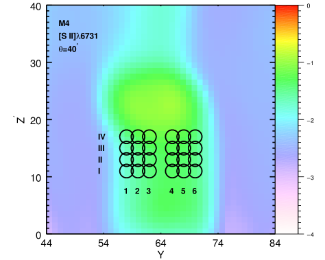
Figure 8.— Normalized and integrated emission line maps for model M1 (left) and M4 (right) for two different lines, [O I]$\lambda 6300$ (left) and [S II]$\lambda 6731$ (right). The jet is inclined $\theta=40^{\circ}$ with respect to the line of sight and the $Y$ and $Z^{\prime}$ coordinates are in code units. The jet inlet is centered at $(y,z)=(64,0)$. In both cases we have superimposed the slit positions (from 1 to 6), symmetrically disposed in both sides of the jet axis, and the four regions (from I to IV).

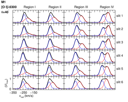
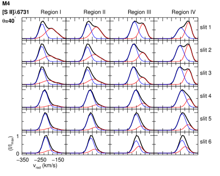
Figure 9.— Line profiles (black solid line) extracted for each slit (slits 1 to 6 from top to bottom, as indicated in the rightmost part of the panels) defined in Figure 8, as well as for each one of the four different regions (from I to IV; from left to right as indicated in the topmost part of the panels) for model M1 (top) and M4 (bottom), for the [O I]$\lambda$6300 (top) and [S II]$\lambda 6731$ (bottom) line profiles (see also Figure 9). Red and blue solid lines represent the profiles for the adjusted gaussians. The intensity in each spectra is normalized to its maximum value and the velocity ranges from -350 km s^-1 to -100 km^-1 (see the left-bottom panel).

References

- Anglada et al. (2007) Anglada, G., López, R., Estalella, R., et al. 2007, AJ, 133, 2799
- Anderson et al. (2003) Anderson, J.M. , Li, Z.-Y., Krasnopolsky, R., & Blandford, R.D., 2003, ApJ, 590, 107
- Bacciotti et al. (2002) Bacciotti, F. , Ray, T.P., Mundt, R., Eisloffel, J., & Solf, J., 2002, ApJ, 576, 222
- Bally et al. (2006) Bally, J., Licht, D., Smith, N., & Walawender, J. 2006, AJ, 131, 473
- Biretta et al. (2016) Biretta, J. et al. 2016, in STIS Instrument Handbook, Version 15.0, (Baltimore: STScI).
- Blandford & Payne (1982) Blandford, R. D., & Payne, D. G. 1982, MNRAS, 199, 883
- Cabrit et al. (2006) Cabrit, S., Pety, J., Pesenti, N., & Dougados, C., 2006, A&A,452, 897
- Canto & Raga (1995) Canto, J., & Raga, A. C. 1995, MNRAS, 277, 1120
- Canto & Raga (1996) Canto, J., & Raga, A. C. 1996, MNRAS, 280, 559
- Cerqueira & de Gouveia Dal Pino (2004) Cerqueira, A.H., & de Gouveia dal Pino, E.M. 2004, A&A, 426, L25
- Cerqueira et al. (2006) Cerqueira, A.H., Velázquez, P.F., Raga, A.C., Vasconcelos, M.J., & De Colle, F., 2006, A&A, 448, 231
- Cerqueira et al. (2015) Cerqueira, A. H., Reyes-Iturbide, J., De Colle, F., & Vasconcelos, M. J. 2015, AJ, 150, 45
- Chrysostomou et al. (2008) Chrysostomou, A., Bacciotti, F., Nisini, B., Ray, T.P., Eisloffel, J., Davis, C.J., & Takami, M., 2008, A&A 482, 575
- Choi et al. (2011) Choi M., Kang, M., & Tatematsu, K. 2011, ApJ, 728, L34
- Ciardi et al. (2008) Ciardi, A., Ampleford, D. J., Lebedev, S. V., & Stehle, C. 2008, ApJ, 678, 968-973
- Codella et al. (2004) Codella, C., Cabrit, S., Gueth, F., Cesaroni, R., Bacciotti, F., Lefloch, B., & McCaughrean, M.J., 2007, A&A, 462, L53
- Coffey et al. (2004) Coffey, D., Bacciotti, F., Woitas, J., Ray, T.P., & Eisloffel, J., 2004, ApJ, 604, 758
- Coffey et al. (2007) Coffey, D., Bacciotti, F., Ray, T.P., Eisloffel, J., & Woitas, J., 2007, ApJ, 663, 350
- Coffey et al. (2008) Coffey, D., Bacciotti, F., & Podio, L., 2008, ApJ, 689, 1112
- Coffey et al. (2011) Coffey, D., Bacciotti, F., Chrysostomou, A., Nisini, B., & Davis, C. 2011, A&A, 526, 40
- Coffey et al. (2012) Coffey, D., Rigliaco, E., Bacciotti, F., Ray, T. P., & Eislöffel, J. 2012, ApJ, 749, 139
- Coffey et al. (2015) Coffey, D., Dougados, C., Cabrit, S., Pety, J., & Bacciotti, F. 2015, ApJ, 804, 2
- Davis et al. (2000) Davis, C.J., Berndsen, A., Smith, M.D., Chrysostomou, A., & Hobson, J., 2000, MNRAS 314, 241
- De Colle et al. (2008) De Colle, F., del Burgo, C., Raga, A.C., 2008, A&A, 485, 765
- De Colle et al. (2010) De Colle, F., del Burgo, C., & Raga, A. C. 2010, ApJ, 721, 929
- Dougados et al. (2000) Dougados, C., Cabrit, S., Lavalley, C., Ménard, F. 2000, A&A, 357, L61
- Fendt (2011) Fendt, C. 2011, ApJ, 737, 43
- Ferreira et al. (2006) Ferreira, J., Dougados, C., & Cabrit, S., 2006, A&A 453, 785–796
- Hartigan & Hillenbrand (2009) Hartigan, P., & Hillenbrand, L. 2009, ApJ, 705, 1388
- Lavalley-Fouquet et al. (2000) Lavalley-Fouquet, C., Cabrit, S., & Dougados, C. 2000, A&A, 356, L41
- Launhardt et al. (2009) Launhardt, R., Pavlyuchenkov, Ya., Gueth, F., Chen, X., Dutrey, A., Guilloteau, S., Henning, Th., Piétu, V., Schreyer, K., Semenov, D. 2009, A&A, 494, 147
- Lee et al. (2007) Lee, C.-F., Ho, P.T.P., Palau, A., Hirano, N., Bourke, T.L., Shang, H., & Zhang, Q., 2007, ApJ, 670, 1188
- Lee et al. (2008) Lee, C.-F., Ho, P.T.P., Bourke, T.L., Hirano, N., Shang, H., & Zhang, Q., 2008, ApJ, 685, 1026
- Li et al. (2014) Li, Z-Y., Banerjee, R., Pudritz, R.E. et al. 2014, in Protostars and Planets VI, University of Arizona Press (2014), eds. H. Beuther, R. Klessen, C. Dullemond, Th. Henning
- Livio (1999) Livio, M. 1999, Physics Reports, 331 (3-5), 225
- Louvet et al. (2016) Louvet, F., Dougados, C., Cabrit, S., et al. 2016, arXiv:1607.08645
- Masciadri & Raga (2001a) Masciadri, E., & Raga, A. C. 2001, A&A, 376, 1073
- Masciadri & Raga (2001b) Masciadri, E., & Raga, A. C. 2001, AJ, 121, 408
- Pech et al. (2012) Pech, G., Zapata, L.A., Loinard, L., & Rodríguez, L.F. 2012, ApJ, 751, 78
- Pesenti et al. (2004) Pesenti, N., Dougados, C., Cabrit, S., Ferreira, J., Casse, F., Garcia, P., & O’Brien, D., 2004, A&A, 416, L9
- Pety et al. (2006) Pety, J., Gueth, F., Guilloteau, S., & Dutrey, A., 2006, A&A, 458, 841
- Pudritz et al. (2007) Pudritz, R.E., Ouyed, R., Fendt, C., & Brandenburg, A., 2007, Protostars and Planets V, 277
- Raga, Navarro-González & Villagrán-Muniz (2000) Raga, A.C., Navarro-González, R. & Villagrán-Muniz, M. 2000, RMxAA, 36, 67
- Raga et al. (2001) Raga, A., Cabrit, S., Dougados, C., & Lavalley, C. 2001, A&A, 367, 959
- Raga et al. (2004) Raga, A.C., Riera, A., Masciadri, E., Beck, T., Böhm, K.H., & Binette, L. 2004, AJ, 127, 1081
- Raga et al. (2007) Raga, A.C., De Colle, F., Kajdic, P., Esquivel, A., & Cantó, J. 2007, A&A, 465, 879
- Reipurth & Bally (2001) Reipurth, B., & Bally, J. 2001, ARA&A, 39, 403
- Shu et al. (2000) Shu, F.H., Najita, J., Shang, H., & Li, Z.-Y., 2000, Protostars and Planets IV, University of Arizona Press, Eds. V. Mannings, A.P. Boss, 789
- Soker (2005) Soker, N., 2005, A&A, 435, 125
- Smith & Rosen (2007) Smith, M.D., Rosen, A., 2007, MNRAS, 378, 691
- Staff et al. (2015) Staff, J.E., Koning, N., Ouyed, R. et al. 2015, MNRAS, 446, 3975
- van Albada, van Leer & Roberts (1982) van Albada, G.D., van Leer, B., & Roberts, W.W.Jr. 1982, A&A, 108, 76
- Yuan & Narayan (2014) Yuan, F. & Narayan, R. 2014, ARA&A, 52, 529
- Woitas et al (2005) Woitas, J., Bacciotti, F., Ray, T.P., Marconi, A., Coffey, D., & Eisloffel, J., 2005, A&A, 432, 149
- Zapata et al. (2015) Zapata, L. A., Lizano, S., Rodríguez, L. F., et al. 2015, ApJ, 798, 131