Analyzing Ozone Conc. by Bayesian Spatio-temporal Quantile Regression

\corraddr

P. Das, Deaprtment of Statistics, North Carolina State University, 2311 Stinson Drive, Raleigh, NC 27695, USA. E-mail: pdas@ncsu.edu

Analyzing Ozone Concentration by Bayesian Spatio-temporal Quantile Regression

P. Das\corrauthΒ and S. Ghosal a b aaaffiliationmark: North Carolina State University, NC 27695, USA
bbaffiliationmark: North Carolina State University, NC 27695, USA
(00 Month 2012; 00 Month 2012; 00 Month 2012)
Abstract

Ground level Ozone is one of the six common air-pollutants on which the EPA has set national air quality standards. In order to capture the spatio-temporal trend of 1-hour and 8-hour average ozone concentration in the US, we develop a method for spatio-temporal simultaneous quantile regression. Unlike existing procedures, in the proposed method, smoothing across the sites is incorporated within modeling assumptions thus allowing borrowing of information across locations, an essential step when the number of samples in each location is low. The quantile function has been assumed to be linear in time and smooth over space and at any given site is given by a convex combination of two monotone increasing functions ΞΎ1subscriptπœ‰1\xi_{1} and ΞΎ2subscriptπœ‰2\xi_{2} not depending on time. A B-spline basis expansion with increasing coefficients varying smoothly over the space is used to put a prior and a Bayesian analysis is performed. We analyze the average daily 1-hour maximum and 8-hour maximum ozone concentration level data of US and California during 2006-2015 using the proposed method. It is noted that in the last ten years, there is an overall decreasing trend in both 1-hour maximum and 8-hour maximum ozone concentration level over the most parts of the US. In California, an overall a decreasing trend of 1-hour maximum ozone level is observed while no particular overall trend has been observed in the case of 8-hour maximum ozone level.

keywords:
B-spline prior; Spatio-temporal quantile regression; Block Metropolis-Hastings; US ozone data.

1 Introduction

In the field of analysis of weather data, greenhouse gas emission data, biological experimental data, MRI scan data, it is of interest to estimate the spatio-temporal dependence structure of the response variable at different levels such as upper and lower extremes. Traditional spatio-temporal mean regression may be inappropriate in this context. For example, if the response variable is highly skewed over the time, spatio-temporal mean regression does not represent a typical relation.

Quantile regression was introduced in Koenkar and Bassett (1978). Generalizations and extensions of quantile regression were proposed from both frequentist and Bayesian perspective (Yu and Moyeed (2001), Kottas and Gelfand (2001), Gelfand and Kottas (2003), Kottas and Krnjajic (2009)). A comprehensive account of various aspects of quantile regression can be found in Koenkar (2005). The above methods were proposed for a single quantile level. The main drawback of separate quantile regression for different levels is that an estimated lower quantile curve may cross an estimated upper quantile curve violating the monotonicity of the quantiles. In addition, a single quantile regression does not allow for joint inference.

Methods addressing the monotonicity issue in estimating multiple quantile regression have also been proposed (He (1997), Neocleous and Portnoy (2008), Takeuchi (2004), Takeuchi etΒ al. (2006), Vapnik (1995), Shim and Lee (2010), Shim etΒ al. (2009), Bondell etΒ al. (2010), Dunson and Taylor (2005)). The non-crossing quantile regression method proposed in Wu and Liu (2009) sequentially updates the quantile curves under the constraint that the higher estimated quantile curves stay above the the lower ones. The problem with this method and the many of the above mentioned non-crossing quantile regression methods is that the estimated values of the quantile curves are dependent on the grid of quantiles where the curves are estimated. For example, using most of the above-mentioned methods, if we estimate the quantile lines for quantile grids T1={0.25,0.5,0.75}subscript𝑇10.250.50.75T_{1}=\{0.25,0.5,0.75\} and T2={0.2,0.5,0.8}subscript𝑇20.20.50.8T_{2}=\{0.2,0.5,0.8\}, the estimates of Ο„=0.5𝜏0.5\tau=0.5 by the two methods would come different, which is not desirable.

Instead of fitting the quantile regression lines for a fixed set of quantiles, a more informative picture emerges by estimating the entire quantile curve (Tokdar and Kadane (2012), Das and Ghosal (2016)). Let Q​(Ο„|x)=inf​{q:P​(Y≀q|X=x)β‰₯Ο„}𝑄conditional𝜏π‘₯infconditional-setπ‘žπ‘ƒπ‘Œconditionalπ‘žπ‘‹π‘₯𝜏Q(\tau|x)=\text{inf}\{q:P(Y\leq q|X=x)\geq\tau\} denote the Ο„πœ\tau-th quantile (0≀τ≀1)0𝜏1(0\leq\tau\leq 1) of a response Yπ‘ŒY at X=x𝑋π‘₯X=x, X𝑋X being the predictor. From Theorem 1 of Tokdar and Kadane (2012) it follows that a linear specification Q​(Ο„|x)=Ξ²0​(Ο„)+x​β1​(Ο„),Ο„βˆˆ[0,1]formulae-sequence𝑄conditional𝜏π‘₯subscript𝛽0𝜏π‘₯subscript𝛽1𝜏𝜏01Q(\tau|x)=\beta_{0}(\tau)+x\beta_{1}(\tau),\;\tau\in[0,1] is monotonically increasing in Ο„πœ\tau for every x∈[0,1]π‘₯01x\in[0,1] if and only if

Q​(Ο„|x)=ΞΌ+γ​x+Οƒ1​x​ξ1​(Ο„)+Οƒ2​(1βˆ’x)​ξ2​(Ο„),𝑄conditional𝜏π‘₯πœ‡π›Ύπ‘₯subscript𝜎1π‘₯subscriptπœ‰1𝜏subscript𝜎21π‘₯subscriptπœ‰2𝜏\displaystyle Q(\tau|x)=\mu+\gamma x+\sigma_{1}x\xi_{1}(\tau)+\sigma_{2}(1-x)\xi_{2}(\tau),

where Οƒ1subscript𝜎1\sigma_{1} and Οƒ2subscript𝜎2\sigma_{2} are some constants and ΞΎ1,ΞΎ2:][0,1]↦[0,1]\xi_{1},\xi_{2}:][0,1]\mapsto[0,1] are monotonically increasing function in Ο„βˆˆ[0,1]𝜏01\tau\in[0,1]. A monotonic transformation of the explanatory and the response variables to unit intervals reduces to this

Q​(Ο„|x)=x​ξ1​(Ο„)+(1βˆ’x)​ξ2​(Ο„),𝑄conditional𝜏π‘₯π‘₯subscriptπœ‰1𝜏1π‘₯subscriptπœ‰2𝜏\displaystyle Q(\tau|x)=x\xi_{1}(\tau)+(1-x)\xi_{2}(\tau), (1)

where ΞΎ1subscriptπœ‰1\xi_{1} and ΞΎ2subscriptπœ‰2\xi_{2} are monotonically increasing bijection from the unit interval to itself. Tokdar and Kadane (2012) took transformed Gaussian process prior to estimate ΞΎ1subscriptπœ‰1\xi_{1} and ΞΎ2subscriptπœ‰2\xi_{2}, while Das and Ghosal (2016) used B-spline basis for that purpose and argued the advantages of using B-spline basis over transformed Gaussian process prior.

Consider the scenario where time is the explanatory variable and the values of the response variables corresponding to time-points are available for different spatial locations. The methods of estimating a single quantile regression curve has been extended to analyze spatial data (Lee and Neocleous (2010), Oh etΒ al. (2011), Sobotka and Kneib (2012)). Various methods for modeling spatially varying distribution function have been proposed in last decade (Dunson and Park (2008), Gelfand etΒ al. (2005), Reich and Fuentes (2007), Griffin and Steel (2006)). As mentioned in Reich (2012), these methods treat the conditional distribution of the response at each spatial location as unknown quantities and are estimated from the data.

One of the first work addressing the non-crossing issue of the spatial quantile regression was proposed in Reich etΒ al. (2011). They proposed a two-stage method and ensured monotonicity of the estimated quantile functions using the Bernstein polynomial basis function. Reich (2012) assumed separate non-crossing quantile functions for each spatial location which evolves over time. Spatial smoothing was performed using Gaussian process priors. Separate analysis for each spatial location may be sensitive to small sample sizes at individual locations. While this method allows estimation at all quantile levels, post-estimation processing step makes the quantification of uncertainty difficult. Instead of estimating the quantile function for a set of grid-points, the estimation of the entire quantile function is more informative. To address the small area estimation problem, instead of assuming unrelated quantile functions for each spatial locations, we assume that the quantile function is smooth over space and linear in time. For any given spatial location, the estimated quantile function has the same form as in Equation (1). Similar to Das and Ghosal (2016), the monotonicity constraint on the curves ΞΎ1subscriptπœ‰1\xi_{1} and ΞΎ2subscriptπœ‰2\xi_{2} are obtained through B-spline basis expansion with coefficients (which are functions of the spatial location) increasing and lying in the unit interval. The coefficients of the B-spline basis expansion over the d𝑑d-dimensional space are modeled by the tensor product of univariate B-splines basis functions. A closed form expression for the likelihood function is obtained in terms of the parameters in d𝑑d independent simplexes whose dimensions depend of the degree of the used B-spline basis functions. Unlike the methods proposed in Reich etΒ al. (2011) and Reich (2012), the main advantage of this method is that once we estimate the parameters of the model, estimated response variable can be found for any spatial location, time and quantiles without further kriging or interpolation, and hence allows proper uncertainty quantification within the Bayesian paradigm. Most importantly, the approach incorporates small area estimation issues automatically in its modeling approach.

2 Ozone in troposphere

Ozone can be naturally found in the troposphere and other parts of the atmosphere. While, more ozone concentration in the stratosphere is desirable as it helps absorb the ultra-violet radiation, higher ozone concentration level in the troposphere is harmful for living beings. Ozone occurs naturally in the troposphere in low concentration. There are mainly two sources of tropospheric ozone. A significant amount of ozone is released by plants and soil. Other than that, sometimes ozone migrates down to the troposphere from the stratosphere. However, the extent of ground-level naturally occurring ozone concentration is not considered a threat to living beings and the environment.

On the other hand, ozone is a byproduct of many human activities. Increasing automobiles and industries are the main source the β€œbad” ozone at the ground-level. As mentioned in an online article111Source http://www.windows2universe.org/earth/Atmosphere/ozone_tropo.html&edu=high, current ground-level ozone concentration has doubled since 1900. Although no single source emits ozone directly, it is generated when the hydrocarbons and nitrogen-oxides, emitted by automobiles, fuel power plants and other industrial machineries, interact with each other in the presence of sunlight, specifically the ultra-violet (UV) ray. In general, ozone level reaches its highest level during the summer season. Typically, in the span of a day, ozone level reaches its highest level during mid and late afternoon.

Recently tropospheric ozone has been related to many health problems and environmental issues. Exposure to higher level of ozone might cause respiratory problems. In plants, it slows down growth and photosynthesis and damages internal cells. High ground-level ozone also damages textile dyes, rubbers and fibers and a few genre of paints.

Because of its unstable nature, there is no existing way to move the tropospheric ozone to the stratosphere which can be thought as the ideal way to deal with this environmental hazard. Under the Clean Air act, the US Environment Protection Agency (EPA) considers tropospheric ozone as one of the six pollutants considered to be harmful to human health and environment. Proposed ozone standards can be found in this site222Source https://www.epa.gov/sites/production/files/2016-04/documents/20151001basicsfs.pdf (accessed 11-26-2016) which says an area would meet the ozone standards if the 4th highest maximum daily 8-hour ozone concentration each year, averaged over three years, is 70 ppb (parts per billion) or below. In this paper, we develop a spatio-temporal quantile regression model for measuring the ozone concentration level over the US and California during the period 2006-2015.

Let Q​(Ο„|x,𝐳)𝑄conditional𝜏π‘₯𝐳Q(\tau|x,\mathbf{z}) denote the Ο„πœ\tau-th quantile of the response variable i.e., ozone concentration level at location 𝐳𝐳\mathbf{z} and time-point xπ‘₯x. We assume a linear dependence structure of the dependent variable on time and the quantile function is smooth over the space. In our model, the quantile function is given by

Q​(Ο„|x,𝐳)=Ξ²0​(Ο„,𝐳)+x​β1​(Ο„,𝐳)​forβ€‹Ο„βˆˆ[0,1].𝑄conditional𝜏π‘₯𝐳subscript𝛽0𝜏𝐳π‘₯subscript𝛽1𝜏𝐳for𝜏01\displaystyle Q(\tau|x,\mathbf{z})=\beta_{0}(\tau,\mathbf{z})+x\beta_{1}(\tau,\mathbf{z})\;\text{for}\;\tau\in[0,1]. (2)

3 Proposed Bayesian Method

Our explanatory variable X𝑋X is time. Let {Xl​i}i=1nlsuperscriptsubscriptsubscript𝑋𝑙𝑖𝑖1subscript𝑛𝑙\{X_{li}\}_{i=1}^{n_{l}} and {Yl​i}i=1nlsuperscriptsubscriptsubscriptπ‘Œπ‘™π‘–π‘–1subscript𝑛𝑙\{Y_{li}\}_{i=1}^{n_{l}} denote the values of X𝑋X and Yπ‘ŒY at location 𝐳l=(z1​l,…,zd​l)subscript𝐳𝑙subscript𝑧1𝑙…subscript𝑧𝑑𝑙\mathbf{z}_{l}=(z_{1l},\ldots,z_{dl}) for l=1,…,L𝑙1…𝐿l=1,\ldots,L, and let nlsubscript𝑛𝑙n_{l} denote the sample size at location 𝐳lsubscript𝐳𝑙\mathbf{z}_{l}. By a monotonic transformation, X𝑋X, Yπ‘ŒY and each coordinates of the spatial locations are transformed to take values in the unit intervals. From Theorem 1 of Tokdar and Kadane (2012), it follows that a linear specification Q​(Ο„|x)=Ξ²0​(Ο„)+x​β1​(Ο„),Ο„βˆˆ[0,1]formulae-sequence𝑄conditional𝜏π‘₯subscript𝛽0𝜏π‘₯subscript𝛽1𝜏𝜏01Q(\tau|x)=\beta_{0}(\tau)+x\beta_{1}(\tau),\;\tau\in[0,1] is monotonically increasing in Ο„πœ\tau for every x∈[0,1]π‘₯01x\in[0,1] if and only if

Q​(Ο„|x)=x​ξ1​(Ο„)+(1βˆ’x)​ξ2​(Ο„)​forβ€‹Ο„βˆˆ[0,1],x∈[0,1]formulae-sequence𝑄conditional𝜏π‘₯π‘₯subscriptπœ‰1𝜏1π‘₯subscriptπœ‰2𝜏for𝜏01π‘₯01\displaystyle Q(\tau|x)=x\xi_{1}(\tau)+(1-x)\xi_{2}(\tau)\;\text{for}\;\tau\in[0,1],\;x\in[0,1] (3)

where ΞΎ1,ΞΎ2:[0,1]↦[0,1]:subscriptπœ‰1subscriptπœ‰2maps-to0101\xi_{1},\xi_{2}:[0,1]\mapsto[0,1] are monotonically increasing in Ο„βˆˆ[0,1]𝜏01\tau\in[0,1]. Let 𝐙=(z1,…,zd),zi∈[0,1]formulae-sequence𝐙subscript𝑧1…subscript𝑧𝑑subscript𝑧𝑖01\mathbf{Z}=(z_{1},\ldots,z_{d}),z_{i}\in[0,1] for i=1,…,d𝑖1…𝑑i=1,\ldots,d, denote the spatial location (site) where the response variable is measured. We assume that the dependence structure of the quantile function at any site 𝐙=𝐳𝐙𝐳\mathbf{Z}=\mathbf{z} is given by

Q​(Ο„|x,𝐳)=x​ξ1​(Ο„,𝐳)+(1βˆ’x)​ξ2​(Ο„,𝐳),Ο„βˆˆ[0,1],x,y∈[0,1],𝐳∈[0,1]d,formulae-sequence𝑄conditional𝜏π‘₯𝐳π‘₯subscriptπœ‰1𝜏𝐳1π‘₯subscriptπœ‰2𝜏𝐳formulae-sequence𝜏01π‘₯formulae-sequence𝑦01𝐳superscript01𝑑\displaystyle Q(\tau|x,\mathbf{z})=x\xi_{1}(\tau,\mathbf{z})+(1-x)\xi_{2}(\tau,\mathbf{z}),\;\tau\in[0,1],\;x,y\in[0,1],\;\mathbf{z}\in[0,1]^{d}, (4)

where ΞΎ1​(β‹…,𝐳),ΞΎ2​(β‹…,𝐳)subscriptπœ‰1⋅𝐳subscriptπœ‰2⋅𝐳\xi_{1}(\cdot,\mathbf{z}),\xi_{2}(\cdot,\mathbf{z}) are monotonic functions from [0,1]01[0,1] to [0,1]01[0,1]. For any fixed 𝐳𝐳\mathbf{z}, equation (4) can be reframed as

Q​(Ο„|x,𝐳)=Ξ²0​(Ο„,𝐳)+x​β1​(Ο„,𝐳),Ο„βˆˆ[0,1],x,y∈[0,1],formulae-sequence𝑄conditional𝜏π‘₯𝐳subscript𝛽0𝜏𝐳π‘₯subscript𝛽1𝜏𝐳formulae-sequence𝜏01π‘₯𝑦01\displaystyle Q(\tau|x,\mathbf{z})=\beta_{0}(\tau,\mathbf{z})+x\beta_{1}(\tau,\mathbf{z}),\;\tau\in[0,1],\;x,y\in[0,1], (5)

where Ξ²0​(Ο„,𝐳)=ΞΎ2​(Ο„,𝐳)subscript𝛽0𝜏𝐳subscriptπœ‰2𝜏𝐳\beta_{0}(\tau,\mathbf{z})=\xi_{2}(\tau,\mathbf{z}) and Ξ²1​(Ο„,𝐳)=ΞΎ1​(Ο„,𝐳)βˆ’ΞΎ2​(Ο„,𝐳)subscript𝛽1𝜏𝐳subscriptπœ‰1𝜏𝐳subscriptπœ‰2𝜏𝐳\beta_{1}(\tau,\mathbf{z})=\xi_{1}(\tau,\mathbf{z})-\xi_{2}(\tau,\mathbf{z}) denote the slope and the intercept of type quantile regression.

A B-spline basis expansion is one of the most convenient approaches for estimating a function on bounded interval. To estimate ΞΎ1​(β‹…,𝐳)subscriptπœ‰1⋅𝐳\xi_{1}(\cdot,\mathbf{z}) and ΞΎ2​(β‹…,𝐳)subscriptπœ‰2⋅𝐳\xi_{2}(\cdot,\mathbf{z}) in Equation (4), we use a B-spline basis expansion. Taking the coefficients of the B-splines basis functions in increasing order we ensure the monotonicity of these two above-mentioned functions and any monotone increasing function can be approximated through a monotone linear combination of B-splines (Boor (2001)). Das and Ghosal (2016) argued the advantages of using B-spline over Gaussian process for estimating the quantile functions. More specifically, using B-splines allows their equation (10) to be solved analytically, significantly reducing the cost of likelihood evaluation compared with Tokdar and Kadane (2012). We use quadratic B-spline because then equation (10), which is crucial for the likelihood evaluation, reduces to a quadratic equation.

3.1 Prior

Let 0=t0<t1<β‹―<tp1=10subscript𝑑0subscript𝑑1β‹―subscript𝑑subscript𝑝110=t_{0}<t_{1}<\cdots<t_{p_{1}}=1 be the equidistant knots on the interval [0,1]01[0,1] such that tiβˆ’tiβˆ’1=1/p1subscript𝑑𝑖subscript𝑑𝑖11subscript𝑝1t_{i}-t_{i-1}=1/p_{1} for i=1,…,p1𝑖1…subscript𝑝1i=1,\ldots,p_{1}. For B-spline of degree m1subscriptπ‘š1m_{1}, the number of basis functions is J1=p1+m1subscript𝐽1subscript𝑝1subscriptπ‘š1J_{1}=p_{1}+m_{1}. Let {Bj,m1​(β‹…)}j=1p1+m1superscriptsubscriptsubscript𝐡𝑗subscriptπ‘š1⋅𝑗1subscript𝑝1subscriptπ‘š1\{B_{j,m_{1}}(\cdot)\}_{j=1}^{p_{1}+m_{1}} be the basis functions of B-splines of degree m1subscriptπ‘š1m_{1} on [0,1]01[0,1] on the above-mentioned equidistant knots. The basis expansion of the quantile functions at site 𝐳𝐳\mathbf{z} is given by the relations

ΞΎ1​(Ο„,𝐳)subscriptπœ‰1𝜏𝐳\displaystyle\xi_{1}(\tau,\mathbf{z}) =βˆ‘j=1p1+m1ΞΈj​(𝐳)​Bj,m1​(Ο„), 0=ΞΈ1​(𝐳)<β‹―<ΞΈp1+m1​(𝐳)=1,formulae-sequenceabsentsuperscriptsubscript𝑗1subscript𝑝1subscriptπ‘š1subscriptπœƒπ‘—π³subscript𝐡𝑗subscriptπ‘š1πœβ€„0subscriptπœƒ1𝐳⋯subscriptπœƒsubscript𝑝1subscriptπ‘š1𝐳1\displaystyle=\sum_{j=1}^{p_{1}+m_{1}}\theta_{j}(\mathbf{z})B_{j,m_{1}}(\tau),\;0=\theta_{1}(\mathbf{z})<\cdots<\theta_{p_{1}+m_{1}}(\mathbf{z})=1,
ΞΎ2​(Ο„,𝐳)subscriptπœ‰2𝜏𝐳\displaystyle\xi_{2}(\tau,\mathbf{z}) =βˆ‘j=1p1+m1Ο•j​(𝐳)​Bj,m1​(Ο„), 0=Ο•1​(𝐳)<β‹―<Ο•p1+m1​(𝐳)=1,formulae-sequenceabsentsuperscriptsubscript𝑗1subscript𝑝1subscriptπ‘š1subscriptitalic-ϕ𝑗𝐳subscript𝐡𝑗subscriptπ‘š1πœβ€„0subscriptitalic-Ο•1𝐳⋯subscriptitalic-Ο•subscript𝑝1subscriptπ‘š1𝐳1\displaystyle=\sum_{j=1}^{p_{1}+m_{1}}\phi_{j}(\mathbf{z})B_{j,m_{1}}(\tau),\;0=\phi_{1}(\mathbf{z})<\cdots<\phi_{p_{1}+m_{1}}(\mathbf{z})=1, (6)

where the coefficients {ΞΈj​(𝐳)}j=1p1+m1superscriptsubscriptsubscriptπœƒπ‘—π³π‘—1subscript𝑝1subscriptπ‘š1\{\theta_{j}(\mathbf{z})\}_{j=1}^{p_{1}+m_{1}} and {Ο•j​(𝐳)}j=1p1+m1superscriptsubscriptsubscriptitalic-ϕ𝑗𝐳𝑗1subscript𝑝1subscriptπ‘š1\{\phi_{j}(\mathbf{z})\}_{j=1}^{p_{1}+m_{1}} are dependent on the spatial location of the data-points. To put priors on {ΞΈj​(𝐳)}j=1k1+m1superscriptsubscriptsubscriptπœƒπ‘—π³π‘—1subscriptπ‘˜1subscriptπ‘š1\{\theta_{j}(\mathbf{z})\}_{j=1}^{k_{1}+m_{1}} and {Ο•j​(𝐳)}j=1k1+m1superscriptsubscriptsubscriptitalic-ϕ𝑗𝐳𝑗1subscriptπ‘˜1subscriptπ‘š1\{\phi_{j}(\mathbf{z})\}_{j=1}^{k_{1}+m_{1}}, we use d𝑑d-fold tensor product of B-spline basis functions. Thus for the spatial location 𝐳=(z1,…,zd)𝐳subscript𝑧1…subscript𝑧𝑑\mathbf{z}=(z_{1},\ldots,z_{d}), the basis expansion is given by

ΞΈj​(𝐳)subscriptπœƒπ‘—π³\displaystyle\theta_{j}(\mathbf{z}) =βˆ‘k1=1p2+m2β€¦β€‹βˆ‘kd=1p2+m2Ξ±j​k1​⋯​kd​Bk1,m2​(z1)​⋯​Bkd,m2​(zd),j=1,…,p2+m2,formulae-sequenceabsentsuperscriptsubscriptsubscriptπ‘˜11subscript𝑝2subscriptπ‘š2…superscriptsubscriptsubscriptπ‘˜π‘‘1subscript𝑝2subscriptπ‘š2subscript𝛼𝑗subscriptπ‘˜1β‹―subscriptπ‘˜π‘‘subscript𝐡subscriptπ‘˜1subscriptπ‘š2subscript𝑧1β‹―subscript𝐡subscriptπ‘˜π‘‘subscriptπ‘š2subscript𝑧𝑑𝑗1…subscript𝑝2subscriptπ‘š2\displaystyle=\sum_{k_{1}=1}^{p_{2}+m_{2}}\ldots\sum_{k_{d}=1}^{p_{2}+m_{2}}\alpha_{jk_{1}\cdots k_{d}}B_{k_{1},m_{2}}(z_{1})\cdots B_{k_{d},m_{2}}(z_{d}),\;j=1,\ldots,p_{2}+m_{2},
Ο•j​(𝐳)subscriptitalic-ϕ𝑗𝐳\displaystyle\phi_{j}(\mathbf{z}) =βˆ‘k1=1p2+m2β€¦β€‹βˆ‘kd=1p2+m2Ξ²j​k1​⋯​kd​Bk1,m2​(z1)​⋯​Bkd,m2​(zd),j=1,…,p2+m2,formulae-sequenceabsentsuperscriptsubscriptsubscriptπ‘˜11subscript𝑝2subscriptπ‘š2…superscriptsubscriptsubscriptπ‘˜π‘‘1subscript𝑝2subscriptπ‘š2subscript𝛽𝑗subscriptπ‘˜1β‹―subscriptπ‘˜π‘‘subscript𝐡subscriptπ‘˜1subscriptπ‘š2subscript𝑧1β‹―subscript𝐡subscriptπ‘˜π‘‘subscriptπ‘š2subscript𝑧𝑑𝑗1…subscript𝑝2subscriptπ‘š2\displaystyle=\sum_{k_{1}=1}^{p_{2}+m_{2}}\ldots\sum_{k_{d}=1}^{p_{2}+m_{2}}\beta_{jk_{1}\cdots k_{d}}B_{k_{1},m_{2}}(z_{1})\cdots B_{k_{d},m_{2}}(z_{d}),\;j=1,\ldots,p_{2}+m_{2},

where {Bk,m2​(β‹…)}k=1p2+m2superscriptsubscriptsubscriptπ΅π‘˜subscriptπ‘š2β‹…π‘˜1subscript𝑝2subscriptπ‘š2\{B_{k,m_{2}}(\cdot)\}_{k=1}^{p_{2}+m_{2}} are B-spline basis functions of degree m2subscriptπ‘š2m_{2} on [0,1]01[0,1] with equidistant knots 0=s1<β‹―<sp2=10subscript𝑠1β‹―subscript𝑠subscript𝑝210=s_{1}<\cdots<s_{p_{2}}=1 and siβˆ’siβˆ’1=1/p2subscript𝑠𝑖subscript𝑠𝑖11subscript𝑝2s_{i}-s_{i-1}=1/p_{2} for i=1,…,p2𝑖1…subscript𝑝2i=1,\ldots,p_{2}. To ensure the constraints of {ΞΈj​(𝐳)}j=1p1+m1superscriptsubscriptsubscriptπœƒπ‘—π³π‘—1subscript𝑝1subscriptπ‘š1\{\theta_{j}(\mathbf{z})\}_{j=1}^{p_{1}+m_{1}} and {Ο•j​(𝐳)}j=1p1+m1superscriptsubscriptsubscriptitalic-ϕ𝑗𝐳𝑗1subscript𝑝1subscriptπ‘š1\{\phi_{j}(\mathbf{z})\}_{j=1}^{p_{1}+m_{1}} mentioned in Equation (6), it is sufficient to ensure the following constraints

0=Ξ±1​k1​⋯​kd<β‹―<Ξ±(p1+m1)​k1​⋯​kd=1, 0=Ξ²1​k1​⋯​kd<β‹―<Ξ²(p1+m1)​k1​⋯​kd=1,formulae-sequence0subscript𝛼1subscriptπ‘˜1β‹―subscriptπ‘˜π‘‘β‹―subscript𝛼subscript𝑝1subscriptπ‘š1subscriptπ‘˜1β‹―subscriptπ‘˜π‘‘1 0subscript𝛽1subscriptπ‘˜1β‹―subscriptπ‘˜π‘‘β‹―subscript𝛽subscript𝑝1subscriptπ‘š1subscriptπ‘˜1β‹―subscriptπ‘˜π‘‘1\displaystyle 0=\alpha_{1k_{1}\cdots k_{d}}<\cdots<\alpha_{(p_{1}+m_{1})k_{1}\cdots k_{d}}=1,\;0=\beta_{1k_{1}\cdots k_{d}}<\cdots<\beta_{(p_{1}+m_{1})k_{1}\cdots k_{d}}=1, (8)

for {k1,…,kd}∈{1,…,(p2+m2)}dsubscriptπ‘˜1…subscriptπ‘˜π‘‘superscript1…subscript𝑝2subscriptπ‘š2𝑑\{k_{1},\ldots,k_{d}\}\in\{1,\ldots,(p_{2}+m_{2})\}^{d}.

Suppose that we have data for L𝐿L spatial sites 𝐳1,…,𝐳Lsubscript𝐳1…subscript𝐳𝐿\mathbf{z}_{1},\ldots,\mathbf{z}_{L} and at the l𝑙l-th site, {Xl​i,Yl​i}i=1nlsuperscriptsubscriptsubscript𝑋𝑙𝑖subscriptπ‘Œπ‘™π‘–π‘–1subscript𝑛𝑙\{X_{li},Y_{li}\}_{i=1}^{n_{l}} denote the values of the explanatory variable (time) and the response variable, nlsubscript𝑛𝑙n_{l} being the number of data-points for l=1,…,L𝑙1…𝐿l=1,\ldots,L, the log-likelihood is given by (see Appendix for the derivation)

βˆ’βˆ‘l=1Lβˆ‘i=1nllog{Xl​iβˆ‘j=2p1+m1ΞΈjβˆ—(𝐳l)Bjβˆ’1,m1βˆ’1(Ο„Xl​i(Yl​i,𝐳l))\displaystyle-\sum_{l=1}^{L}\sum_{i=1}^{n_{l}}\log\bigg{\{}X_{li}\sum_{j=2}^{p_{1}+m_{1}}\theta^{*}_{j}(\mathbf{z}_{l})B_{j-1,m_{1}-1}(\tau_{X_{li}}(Y_{li},\mathbf{z}_{l}))
+(1βˆ’Xl​i)βˆ‘j=2p1+m1Ο•jβˆ—(𝐳l)Bjβˆ’1,m1βˆ’1(Ο„Xl​i(Yl​i,𝐳l))},\displaystyle+(1-X_{li})\sum_{j=2}^{p_{1}+m_{1}}\phi^{*}_{j}(\mathbf{z}_{l})B_{j-1,m_{1}-1}(\tau_{X_{li}}(Y_{li},\mathbf{z}_{l}))\bigg{\}}, (9)

where

ΞΈjβˆ—β€‹(𝐳)=(p1+m1)​(ΞΈj​(𝐳)βˆ’ΞΈjβˆ’1​(𝐳)),Ο•jβˆ—β€‹(𝐳)=(p1+m1)​(Ο•j​(𝐳)βˆ’Ο•jβˆ’1​(𝐳)),formulae-sequencesubscriptsuperscriptπœƒπ‘—π³subscript𝑝1subscriptπ‘š1subscriptπœƒπ‘—π³subscriptπœƒπ‘—1𝐳subscriptsuperscriptitalic-ϕ𝑗𝐳subscript𝑝1subscriptπ‘š1subscriptitalic-ϕ𝑗𝐳subscriptitalic-ϕ𝑗1𝐳\displaystyle\theta^{*}_{j}(\mathbf{z})=(p_{1}+m_{1})(\theta_{j}(\mathbf{z})-\theta_{j-1}(\mathbf{z})),\;\phi^{*}_{j}(\mathbf{z})=(p_{1}+m_{1})(\phi_{j}(\mathbf{z})-\phi_{j-1}(\mathbf{z})),

for j=2,…,p1+m1𝑗2…subscript𝑝1subscriptπ‘š1j=2,\ldots,p_{1}+m_{1}. and Ο„Xl​i​(Yl​i,𝐳l)subscript𝜏subscript𝑋𝑙𝑖subscriptπ‘Œπ‘™π‘–subscript𝐳𝑙\tau_{X_{li}}(Y_{li},\mathbf{z}_{l}) is the solution of

Yl​i=Xl​i​ξ1​(Ο„,𝐳l)+(1βˆ’Xl​i)​ξ2​(Ο„,𝐳l).subscriptπ‘Œπ‘™π‘–subscript𝑋𝑙𝑖subscriptπœ‰1𝜏subscript𝐳𝑙1subscript𝑋𝑙𝑖subscriptπœ‰2𝜏subscript𝐳𝑙\displaystyle Y_{li}=X_{li}\xi_{1}(\tau,\mathbf{z}_{l})+(1-X_{li})\xi_{2}(\tau,\mathbf{z}_{l}). (10)

The parameters of the log-likelihood are given by Equation (8). We note that once we fix the values of k1,…,kdsubscriptπ‘˜1…subscriptπ‘˜π‘‘k_{1},\ldots,k_{d}, the vector of spacings of the coefficients Ξ±1​k1​⋯​kd,subscript𝛼1subscriptπ‘˜1β‹―subscriptπ‘˜π‘‘\alpha_{1k_{1}\cdots k_{d}}, …,…\ldots, Ξ±(p1+m1)​k1​⋯​kdsubscript𝛼subscript𝑝1subscriptπ‘š1subscriptπ‘˜1β‹―subscriptπ‘˜π‘‘\alpha_{(p_{1}+m_{1})k_{1}\cdots k_{d}} lie on the unit simplex. The same is true for Ξ²1​k1​⋯​kd,subscript𝛽1subscriptπ‘˜1β‹―subscriptπ‘˜π‘‘\beta_{1k_{1}\cdots k_{d}}, …,…\ldots, Ξ²(p1+m1)​k1​⋯​kdsubscript𝛽subscript𝑝1subscriptπ‘š1subscriptπ‘˜1β‹―subscriptπ‘˜π‘‘\beta_{(p_{1}+m_{1})k_{1}\cdots k_{d}}. Define

Ξ³j​k1​⋯​kd=Ξ±(j+1)​k1​⋯​kdβˆ’Ξ±j​k1​⋯​kd,Ξ΄j​k1​⋯​kd=Ξ²(j+1)​k1​⋯​kdβˆ’Ξ²j​k1​⋯​kd,formulae-sequencesubscript𝛾𝑗subscriptπ‘˜1β‹―subscriptπ‘˜π‘‘subscript𝛼𝑗1subscriptπ‘˜1β‹―subscriptπ‘˜π‘‘subscript𝛼𝑗subscriptπ‘˜1β‹―subscriptπ‘˜π‘‘subscript𝛿𝑗subscriptπ‘˜1β‹―subscriptπ‘˜π‘‘subscript𝛽𝑗1subscriptπ‘˜1β‹―subscriptπ‘˜π‘‘subscript𝛽𝑗subscriptπ‘˜1β‹―subscriptπ‘˜π‘‘\displaystyle\gamma_{jk_{1}\cdots k_{d}}=\alpha_{(j+1)k_{1}\cdots k_{d}}-\alpha_{jk_{1}\cdots k_{d}},\;\delta_{jk_{1}\cdots k_{d}}=\beta_{(j+1)k_{1}\cdots k_{d}}-\beta_{jk_{1}\cdots k_{d}}, (11)

for j=1,…,p1+m1βˆ’1𝑗1…subscript𝑝1subscriptπ‘š11j=1,\ldots,p_{1}+m_{1}-1 and {k1,…,kd}∈{1,…,(p2+m2)}dsubscriptπ‘˜1…subscriptπ‘˜π‘‘superscript1…subscript𝑝2subscriptπ‘š2𝑑\{k_{1},\ldots,k_{d}\}\in\{1,\ldots,(p_{2}+m_{2})\}^{d}. Hence for each combination of {k1,…,kd}∈{1,…,(p2+m2)}dsubscriptπ‘˜1…subscriptπ‘˜π‘‘superscript1…subscript𝑝2subscriptπ‘š2𝑑\{k_{1},\ldots,k_{d}\}\in\{1,\ldots,(p_{2}+m_{2})\}^{d}, we have

βˆ‘j=1p1+m1βˆ’1Ξ³j​k1​⋯​kd=1​and​γj​k1​⋯​kdβ‰₯0,βˆ‘j=1p1+m1βˆ’1Ξ΄j​k1​⋯​kd=1​and​δj​k1​⋯​kdβ‰₯0.formulae-sequencesuperscriptsubscript𝑗1subscript𝑝1subscriptπ‘š11subscript𝛾𝑗subscriptπ‘˜1β‹―subscriptπ‘˜π‘‘1andsubscript𝛾𝑗subscriptπ‘˜1β‹―subscriptπ‘˜π‘‘0superscriptsubscript𝑗1subscript𝑝1subscriptπ‘š11subscript𝛿𝑗subscriptπ‘˜1β‹―subscriptπ‘˜π‘‘1andsubscript𝛿𝑗subscriptπ‘˜1β‹―subscriptπ‘˜π‘‘0\displaystyle\sum_{j=1}^{p_{1}+m_{1}-1}\gamma_{jk_{1}\cdots k_{d}}=1\;\text{and}\;\gamma_{jk_{1}\cdots k_{d}}\geq 0,\;\sum_{j=1}^{p_{1}+m_{1}-1}\delta_{jk_{1}\cdots k_{d}}=1\;\text{and}\;\delta_{jk_{1}\cdots k_{d}}\geq 0. (12)

Thus we note that the parameters of the log-likelihood can be divided into 2Γ—(p2+m2)d2superscriptsubscript𝑝2subscriptπ‘š2𝑑2\times(p_{2}+m_{2})^{d} unit simplex blocks. We consider uniform Dirichlet prior on the unit simplex blocks {Ξ³j​k1​⋯​kd}j=1p1+m1βˆ’1superscriptsubscriptsubscript𝛾𝑗subscriptπ‘˜1β‹―subscriptπ‘˜π‘‘π‘—1subscript𝑝1subscriptπ‘š11\{\gamma_{jk_{1}\cdots k_{d}}\}_{j=1}^{p_{1}+m_{1}-1} and {Ξ΄j​k1​⋯​kd}j=1p1+m1βˆ’1superscriptsubscriptsubscript𝛿𝑗subscriptπ‘˜1β‹―subscriptπ‘˜π‘‘π‘—1subscript𝑝1subscriptπ‘š11\{\delta_{jk_{1}\cdots k_{d}}\}_{j=1}^{p_{1}+m_{1}-1} for {k1,…,kd}∈{1,…,(p2+m2)}dsubscriptπ‘˜1…subscriptπ‘˜π‘‘superscript1…subscript𝑝2subscriptπ‘š2𝑑\{k_{1},\ldots,k_{d}\}\in\{1,\ldots,(p_{2}+m_{2})\}^{d}. As mentioned in the earlier section, m1subscriptπ‘š1m_{1} is taken to be 2. The degree of the basis functions corresponding to each spatial coordinates has been considered to be cubic (i.e., m2=3subscriptπ‘š23m_{2}=3).

4 Simulation study

In this section we compare the estimation performance estimation of the proposed method, i.e., Spline Spatio-temporal Quantile Regression (SSTQR) with piece-wise Gaussian Basis function Spatio-temporal Quantile Regression (GBSTQR) (Reich (2012)) based on simulation. For the proposed SSTQR method, we consider both likelihood based and Bayesian approaches. Finding the maximum likelihood estimate (MLE) can be seen as an optimization problem of maximizing an objective function of a constrained parameter space which is given by a collection of unit simplex blocks. Since the evaluation of the likelihood involves integration and linear search, it is hard to check whether the likelihood function is convex or not. Instead of using convex optimization algorithms, global or non-convex optimization algorithms are more reasonable in this scenario. Das (2016b) proposed an efficient global optimization technique on a hyper-rectangular parameter space which has been shown to work faster and than existing global optimization techniques, namely Genetic Algorithm (Fraser (1957), Bethke (1980), Goldberg (1989)) and Simulated annealing (Kirkpatrick etΒ al. (1983), Granville etΒ al. (1994)) yielding better solutions. Das (2016c) modified that algorithm for the case where the sample space is given by an unit simplex. Following that paper, Das (2016a) proposed β€˜Greedy Coordinate Descent of Varying Step sizes on Multiple Simplexes’ (GCDVSMS) algorithm which efficiently minimizes any non-convex (or, maximizes any non-concave) objective function of parameters given by a collection of unit simplex blocks. The main idea of GCDVSMS algorithm is making jumps of varying step-sizes within each unit simplex blocks parallelly and searching for the most favorable direction of movement. In this algorithm, every time a local solution is found, coordinate-wise jumps of various step-sizes are performed until a better solution is found. To find the MLE in this case, GCDVSMS algorithm is used. The values of the tuning parameters in GCDVSMS algorithm are chosen as follows; initial global step size sinitial=1subscript𝑠initial1s_{\text{initial}}=1, step decay rate for the first run ρ1=2subscript𝜌12\rho_{1}=2, step decay rate for other runs ρ2=1.5subscript𝜌21.5\rho_{2}=1.5, step size threshold Ο•=10βˆ’1italic-Ο•superscript101\phi=10^{-1}, sparsity threshold Ξ»=10βˆ’2πœ†superscript102\lambda=10^{-2}, the convergence criteria controlling parameters tol_fun_1=tol_fun_2=10βˆ’1absentsuperscript101=10^{-1}, maximum number of iterations inside each run max_iter=5000max_iter5000\textit{max\_iter}=5000, maximum number of allowed runs max_runs=200max_runs200\textit{max\_runs}=200.

We consider the spatial locations are uniformly distributed over the unit square i.e., [0,1]2superscript012[0,1]^{2}. Number of spatial locations is taken to be L=50𝐿50L=50. For simulation purpose, three different numbers of equidistant temporal data-points for each site have been considered which are n=5,10,20𝑛51020n=5,10,20 (note that, nl=nsubscript𝑛𝑙𝑛n_{l}=n for l=1,…,50𝑙1…50l=1,\ldots,50). Let {𝐳l}l=1Lsuperscriptsubscriptsubscript𝐳𝑙𝑙1𝐿\{\mathbf{z}_{l}\}_{l=1}^{L} denote the spatial locations of the available sites of data where 𝐳l=(zl​1,zl​2)subscript𝐳𝑙subscript𝑧𝑙1subscript𝑧𝑙2\mathbf{z}_{l}=(z_{l1},z_{l2}) is a two-tuple such that 0≀zl​1,zl​2≀1formulae-sequence0subscript𝑧𝑙1subscript𝑧𝑙210\leq z_{l1},z_{l2}\leq 1 for l=1,…,L𝑙1…𝐿l=1,\ldots,L. Consider the spatial quantile function Q​(Ο„|x,𝐳)=x​ξ1​(Ο„,𝐳)+(1βˆ’x)​ξ2​(Ο„,𝐳)𝑄conditional𝜏π‘₯𝐳π‘₯subscriptπœ‰1𝜏𝐳1π‘₯subscriptπœ‰2𝜏𝐳Q(\tau|x,\mathbf{z})=x\xi_{1}(\tau,\mathbf{z})+(1-x)\xi_{2}(\tau,\mathbf{z}) where

ΞΎ1​(Ο„,𝐳)=subscriptπœ‰1𝜏𝐳absent\displaystyle\xi_{1}(\tau,\mathbf{z})= (1βˆ’π³l​1+𝐳l​22)​τ2+𝐳l​1​log⁑(1+Ο„)2​log⁑(2)+𝐳l​22​τ3,1subscript𝐳𝑙1subscript𝐳𝑙22superscript𝜏2subscript𝐳𝑙11𝜏22subscript𝐳𝑙22superscript𝜏3\displaystyle(1-\frac{\mathbf{z}_{l1}+\mathbf{z}_{l2}}{2})\tau^{2}+\mathbf{z}_{l1}\frac{\log(1+\tau)}{2\log(2)}+\frac{\mathbf{z}_{l2}}{2}\tau^{3},
ΞΎ2​(Ο„,𝐳)=subscriptπœ‰2𝜏𝐳absent\displaystyle\xi_{2}(\tau,\mathbf{z})= (1βˆ’π³l​22)​sin⁑(π​τ2)+𝐳l​22​(eΟ„βˆ’1)(eβˆ’1).1superscriptsubscript𝐳𝑙22πœ‹πœ2superscriptsubscript𝐳𝑙22superscriptπ‘’πœ1𝑒1\displaystyle(1-\mathbf{z}_{l2}^{2})\sin(\frac{\pi\tau}{2})+\mathbf{z}_{l2}^{2}\frac{(e^{\tau}-1)}{(e-1)}. (13)

Note that for any given 𝐳∈[0,1]2𝐳superscript012\mathbf{z}\in[0,1]^{2}, ΞΎ1​(β‹…,𝐳)subscriptπœ‰1⋅𝐳\xi_{1}(\cdot,\mathbf{z}) and ΞΎ1​(β‹…,𝐳)subscriptπœ‰1⋅𝐳\xi_{1}(\cdot,\mathbf{z}) are strictly increasing function from [0,1]01[0,1] to [0,1]01[0,1] satisfying ΞΎ1​(0,𝐳)=ΞΎ2​(0,𝐳)=0subscriptπœ‰10𝐳subscriptπœ‰20𝐳0\xi_{1}(0,\mathbf{z})=\xi_{2}(0,\mathbf{z})=0 and ΞΎ1​(1,𝐳)=ΞΎ2​(1,𝐳)=1subscriptπœ‰11𝐳subscriptπœ‰21𝐳1\xi_{1}(1,\mathbf{z})=\xi_{2}(1,\mathbf{z})=1. Since the quantile function is the inverse of the cumulative distribution function, taking U∼U​(0,1)similar-toπ‘ˆπ‘ˆ01U\sim U(0,1), Q​(U|x,𝐳)𝑄conditionalπ‘ˆπ‘₯𝐳Q(U|x,\mathbf{z}) has conditional quantile function Q​(Ο„|x,𝐳)𝑄conditional𝜏π‘₯𝐳Q(\tau|x,\mathbf{z}). For each locations {𝐳l}l=1Lsuperscriptsubscriptsubscript𝐳𝑙𝑙1𝐿\{\mathbf{z}_{l}\}_{l=1}^{L}, we considered the same set of equidistant time-points such that 0=xl​1<β‹―<xl​n=10subscriptπ‘₯𝑙1β‹―subscriptπ‘₯𝑙𝑛10=x_{l1}<\cdots<x_{ln}=1 and (xl​iβˆ’xl​(iβˆ’1))=1/(nβˆ’1)subscriptπ‘₯𝑙𝑖subscriptπ‘₯𝑙𝑖11𝑛1(x_{li}-x_{l(i-1)})=1/(n-1) for i=2,…,n𝑖2…𝑛i=2,\ldots,n. We simulate the response variable Yπ‘ŒY using the equation

yl​i=xl​i​ξ1​(Ul​i,𝐳l)+(1βˆ’xl​i)​ξ2​(Ul​i,𝐳l),l=1,…,L,i=1,…,n.formulae-sequencesubscript𝑦𝑙𝑖subscriptπ‘₯𝑙𝑖subscriptπœ‰1subscriptπ‘ˆπ‘™π‘–subscript𝐳𝑙1subscriptπ‘₯𝑙𝑖subscriptπœ‰2subscriptπ‘ˆπ‘™π‘–subscript𝐳𝑙formulae-sequence𝑙1…𝐿𝑖1…𝑛\displaystyle y_{li}=x_{li}\xi_{1}(U_{li},\mathbf{z}_{l})+(1-x_{li})\xi_{2}(U_{li},\mathbf{z}_{l}),\;l=1,\ldots,L,\;i=1,\ldots,n.

where Ul​i∼U​(0,1)similar-tosubscriptπ‘ˆπ‘™π‘–π‘ˆ01U_{li}\sim U(0,1) for l=1,…,L,i=1,…,nformulae-sequence𝑙1…𝐿𝑖1…𝑛l=1,\ldots,L,\;i=1,\ldots,n. Using both methods, for each of the locations with the number of data-points n=5,10,20𝑛51020n=5,10,20, the quantile curves are estimated for the quantiles {Ο„t}t=1Tsuperscriptsubscriptsubscriptπœπ‘‘π‘‘1𝑇\{\tau_{t}\}_{t=1}^{T} where Ο„t=0.05​tsubscriptπœπ‘‘0.05𝑑\tau_{t}=0.05t and T=19𝑇19T=19. The above-mentioned simulation study is repeated S=50𝑆50S=50 times under different random number generating seeds. Let at the s𝑠s-th simulation study with fixed number of data-points (n=5,10,20𝑛51020n=5,10,20) at each site, the estimated intercept and slope at Ο„tsubscriptπœπ‘‘\tau_{t}-th quantile and location 𝐳lsubscript𝐳𝑙\mathbf{z}_{l} are Ξ²^0(s)​(Ο„t,𝐳l)superscriptsubscript^𝛽0𝑠subscriptπœπ‘‘subscript𝐳𝑙\hat{\beta}_{0}^{(s)}(\tau_{t},\mathbf{z}_{l}) and Ξ²^1(s)​(Ο„t,𝐳l)superscriptsubscript^𝛽1𝑠subscriptπœπ‘‘subscript𝐳𝑙\hat{\beta}_{1}^{(s)}(\tau_{t},\mathbf{z}_{l}) respectively for s=1,…,S𝑠1…𝑆s=1,\ldots,S, t=1,…,T𝑑1…𝑇t=1,\ldots,T and l=1,…,L𝑙1…𝐿l=1,\ldots,L. Q​(Ο„t|x,𝐳l)𝑄conditionalsubscriptπœπ‘‘π‘₯subscript𝐳𝑙Q(\tau_{t}|x,\mathbf{z}_{l}) denotes the true value of the Ο„tsubscriptπœπ‘‘\tau_{t}-th quantile at location 𝐳lsubscript𝐳𝑙\mathbf{z}_{l} at time-point X=x𝑋π‘₯X=x and Q^1(s)​(Ο„t|x,𝐳l)superscriptsubscript^𝑄1𝑠conditionalsubscriptπœπ‘‘π‘₯subscript𝐳𝑙\hat{Q}_{1}^{(s)}(\tau_{t}|x,\mathbf{z}_{l}) is the estimated value of it based on s𝑠s-th simulation study. Then the average of mean squared error (MSE) of the slope, intercept and the quantile value at a given time-point X=x𝑋π‘₯X=x are given by

T1=subscript𝑇1absent\displaystyle T_{1}= 1S​L​Tβ€‹βˆ‘s=1Sβˆ‘l=1Lβˆ‘t=1T(Ξ²0​(Ο„t,𝐳l)βˆ’Ξ²^0(s)​(Ο„t,𝐳l))21𝑆𝐿𝑇superscriptsubscript𝑠1𝑆superscriptsubscript𝑙1𝐿superscriptsubscript𝑑1𝑇superscriptsubscript𝛽0subscriptπœπ‘‘subscript𝐳𝑙superscriptsubscript^𝛽0𝑠subscriptπœπ‘‘subscript𝐳𝑙2\displaystyle\frac{1}{SLT}\sum_{s=1}^{S}\sum_{l=1}^{L}\sum_{t=1}^{T}(\beta_{0}(\tau_{t},\mathbf{z}_{l})-\hat{\beta}_{0}^{(s)}(\tau_{t},\mathbf{z}_{l}))^{2}
T2=subscript𝑇2absent\displaystyle T_{2}= 1S​L​Tβ€‹βˆ‘s=1Sβˆ‘l=1Lβˆ‘t=1T(Ξ²1​(Ο„t,𝐳l)βˆ’Ξ²^1(s)​(Ο„t,𝐳l))21𝑆𝐿𝑇superscriptsubscript𝑠1𝑆superscriptsubscript𝑙1𝐿superscriptsubscript𝑑1𝑇superscriptsubscript𝛽1subscriptπœπ‘‘subscript𝐳𝑙superscriptsubscript^𝛽1𝑠subscriptπœπ‘‘subscript𝐳𝑙2\displaystyle\frac{1}{SLT}\sum_{s=1}^{S}\sum_{l=1}^{L}\sum_{t=1}^{T}(\beta_{1}(\tau_{t},\mathbf{z}_{l})-\hat{\beta}_{1}^{(s)}(\tau_{t},\mathbf{z}_{l}))^{2}
Tx=subscript𝑇π‘₯absent\displaystyle T_{x}= 1S​L​Tβ€‹βˆ‘s=1Sβˆ‘l=1Lβˆ‘t=1T(Q​(Ο„t|x,𝐳l)βˆ’Q^(s)​(Ο„t|x,𝐳l))2.1𝑆𝐿𝑇superscriptsubscript𝑠1𝑆superscriptsubscript𝑙1𝐿superscriptsubscript𝑑1𝑇superscript𝑄conditionalsubscriptπœπ‘‘π‘₯subscript𝐳𝑙superscript^𝑄𝑠conditionalsubscriptπœπ‘‘π‘₯subscript𝐳𝑙2\displaystyle\frac{1}{SLT}\sum_{s=1}^{S}\sum_{l=1}^{L}\sum_{t=1}^{T}(Q(\tau_{t}|x,\mathbf{z}_{l})-\hat{Q}^{(s)}(\tau_{t}|x,\mathbf{z}_{l}))^{2}.
Sample size (per site) Methods MSE
Ξ²0​(Ο„,𝐳)subscript𝛽0𝜏𝐳\beta_{0}(\tau,\mathbf{z}) Ξ²1​(Ο„,𝐳)subscript𝛽1𝜏𝐳\beta_{1}(\tau,\mathbf{z}) Q​(Ο„|0.2,𝐳)𝑄conditional𝜏0.2𝐳Q(\tau|0.2,\mathbf{z}) Q​(Ο„|0.5,𝐳)𝑄conditional𝜏0.5𝐳Q(\tau|0.5,\mathbf{z}) Q​(Ο„|0.8,𝐳)𝑄conditional𝜏0.8𝐳Q(\tau|0.8,\mathbf{z})
n=5𝑛5n=5 SSTQR (ML) 0.0265 0.0437 0.0194 0.0154 0.0192
SSTQR (Bayes) 0.0410 0.0162 0.0103 0.0076 0.0122
GBSTQR 0.2014 0.0349 0.0471 0.1159 0.2209
n=10𝑛10n=10 SSTQR (ML) 0.0248 0.0340 0.0187 0.0146 0.0166
SSTQR (Bayes) 0.0290 0.0127 0.0081 0.0055 0.0082
GBSTQR 0.6000 0.0241 0.0658 0.2337 0.5097
n=20𝑛20n=20 QSSTQR (ML) 0.0186 0.0239 0.0145 0.0119 0.0136
SSTQR (Bayes) 0.0154 0.0100 0.0072 0.0052 0.0061
GBSTQR 0.0685 0.0171 0.0165 0.0398 0.0754
Table 1: Average MSE (based on S=50𝑆50S=50 repetitions of simulation study) of estimated slope, intercept and estimated quantile function value at three time-points X=0.2,0.5,0.8𝑋0.20.50.8X=0.2,0.5,0.8 using SSTQR (both MLE based and Bayesian approach) and GBSTQR over all L=50𝐿50L=50 locations and T=19𝑇19T=19 quantile levels Ο„=0.05,0.10,…,0.95𝜏0.050.10…0.95\tau=0.05,0.10,\ldots,0.95.

For SSTQR (Bayes) method, 10000 iterations are performed and the first 1000 iterations are disregarded as burn-in. In the Table (1), the comparison of average MSE of estimated slope, intercept and estimated quantile curve value at three time-points X=0.2,0.5,0.8𝑋0.20.50.8X=0.2,0.5,0.8 over all locations are provided for both of the above-mentioned methods. Since we are using quadratic B-spline for the quantile basis functions and cubic B-spline for the coordinate-wise spatial basis functions, m1=2subscriptπ‘š12m_{1}=2, m2=3subscriptπ‘š23m_{2}=3. To select the optimum number of knots, we use the Akaike information criterion (AIC). In this simulation study, we consider the cases p1=p2=3,4,5,6formulae-sequencesubscript𝑝1subscript𝑝23456p_{1}=p_{2}=3,4,5,6 and selected the model with best value of AIC.

It is noted that both SSTQR (Bayes) and SSTQR (ML) perform generally better than GBSTQR. SSTQR (Bayes) performs slightly better than SSTQR (ML) which beats the GBSTQR method in performance. It should be also noted that the optimization in the ML estimation can be considerably more challenging than obtaining samples since the negative likelihood is possibly non-convex with multiple local maxima. To find the ML estimate, we solve 250-1024 dimensional constrained black-box optimization problem (for p1,p2=3,4,5,6formulae-sequencesubscript𝑝1subscript𝑝23456p_{1},p_{2}=3,4,5,6).

5 Analysis of ozone concentration data of the US

Ozone concentration data of the US over the last several years can be found at the US EPA website333Source https://www3.epa.gov/airquality/airdata/ad_data.html. The yearly averages of the daily maximum of observed hourly ozone concentration values between 9:00 AM and 8:00 PM (Daily 1-hour maximum average ozone concentration) and the daily maximum of 8 hour running average of observed hourly ozone concentration values (Daily 8-hour maximum average ozone concentration) have been collected at around 1629 sites all over the US in the last several years. As mentioned in the EPA website444Sourcehttps://www3.epa.gov/region1/airquality/avg8hr.html, in 1997, EPA replaced the previous 1-hour ozone standard with 8-hour standard (which is supposed to be more protective) at a level of 84 parts per billion (ppb). 8-hour primary standard is considered to be met at any given site if the 3-year mean of the annual fourth-highest daily maximum 8-hour average ozone concentration is less than or equal to the proposed level, i.e., 84 ppb as per EPA standard announced in 1997. Later in 2008, EPA changed the 8-hour ozone concentration standard to 75 ppb and in 2015, it was decreased to 70 ppb due to emergence of more scientific evidence regarding the effects of ozone on public health and welfare. As mentioned in a news article Barboza (2015), environmentalists and health advocacy groups including the American Lung Association endorsed 8-hour ozone standard to be 60 ppb. But Barboza (2015) mentioned as per EPA data from 2014, more than 40 million people, or in other words, about 1 in every 8 people of the US lives in the counties with air pollution levels exceeding the previous ozone standard of 75 ppb.

Here an analysis of the spatio-temporal trend of daily 1-hour maximum average and daily 8-hour maximum average ozone concentration for the last 10 years, i.e., during the period 2006-2015, has been provided using the proposed method. It should be noted that in the given dataset, each site does not have the data for all the years considered while some of the sites have multiple observations recorded at the same year measured using different measuring instruments. With the proposed method, these cases can be handled automatically without any further required modifications. For the analysis, the Markov Chain Monte Carlo (MCMC) has been initialized at the SSTQR (ML) estimate obtained using the GCDVSMS algorithm proposed in Das (2016a) with the values of the tuning parameters as mentioned in the earlier section. For this analysis, 10000 iterations have been performed disregarding the first 1000 iterations as burn-in. The number of knots of the B-spline basis functions has been chosen based on the AIC criterion as mentioned in Section 4.
Refer to caption
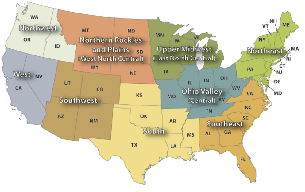
Figure 1: Climate region-wise division of the US.

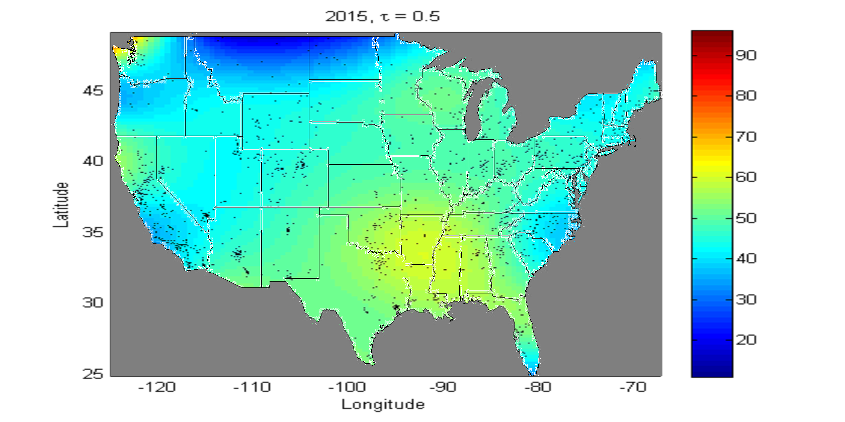
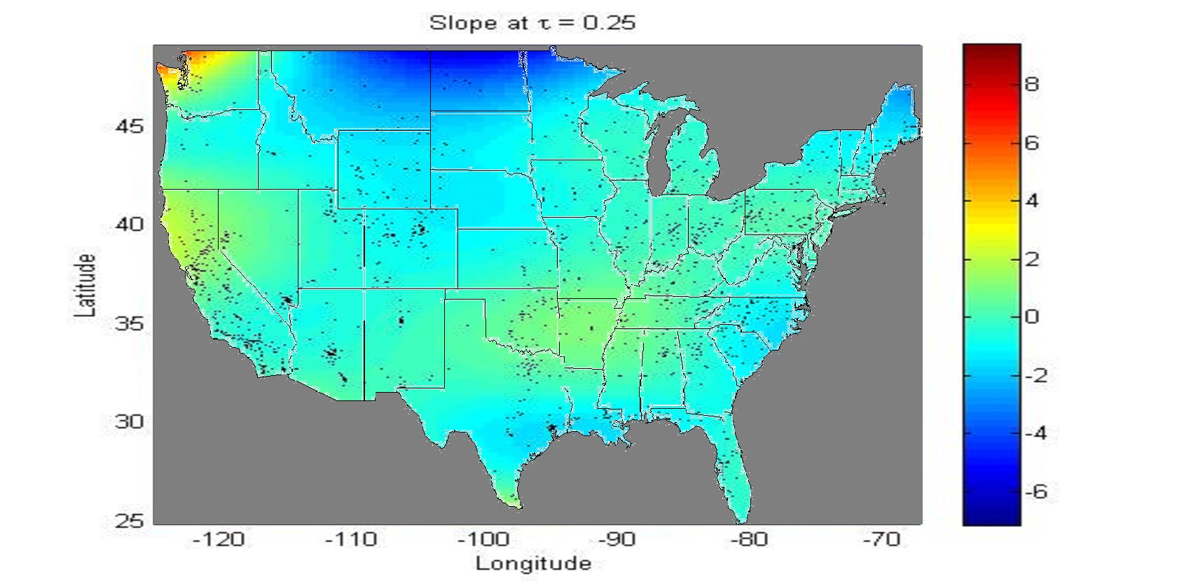
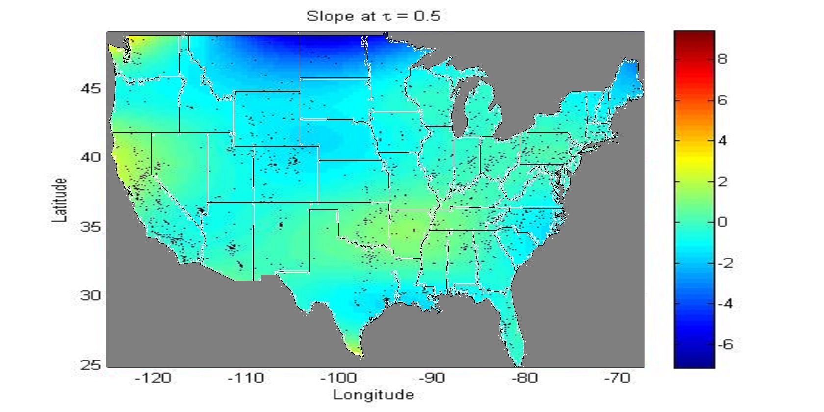
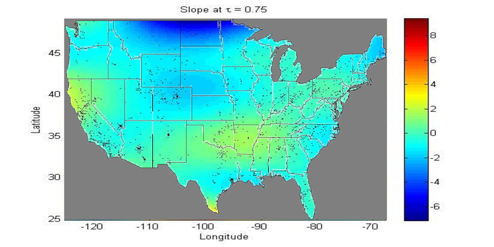
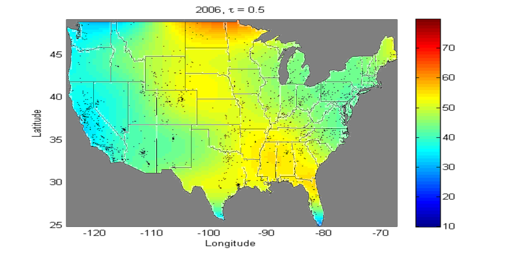
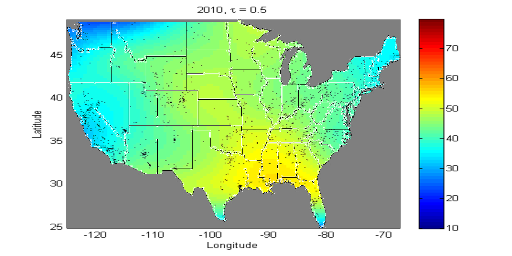
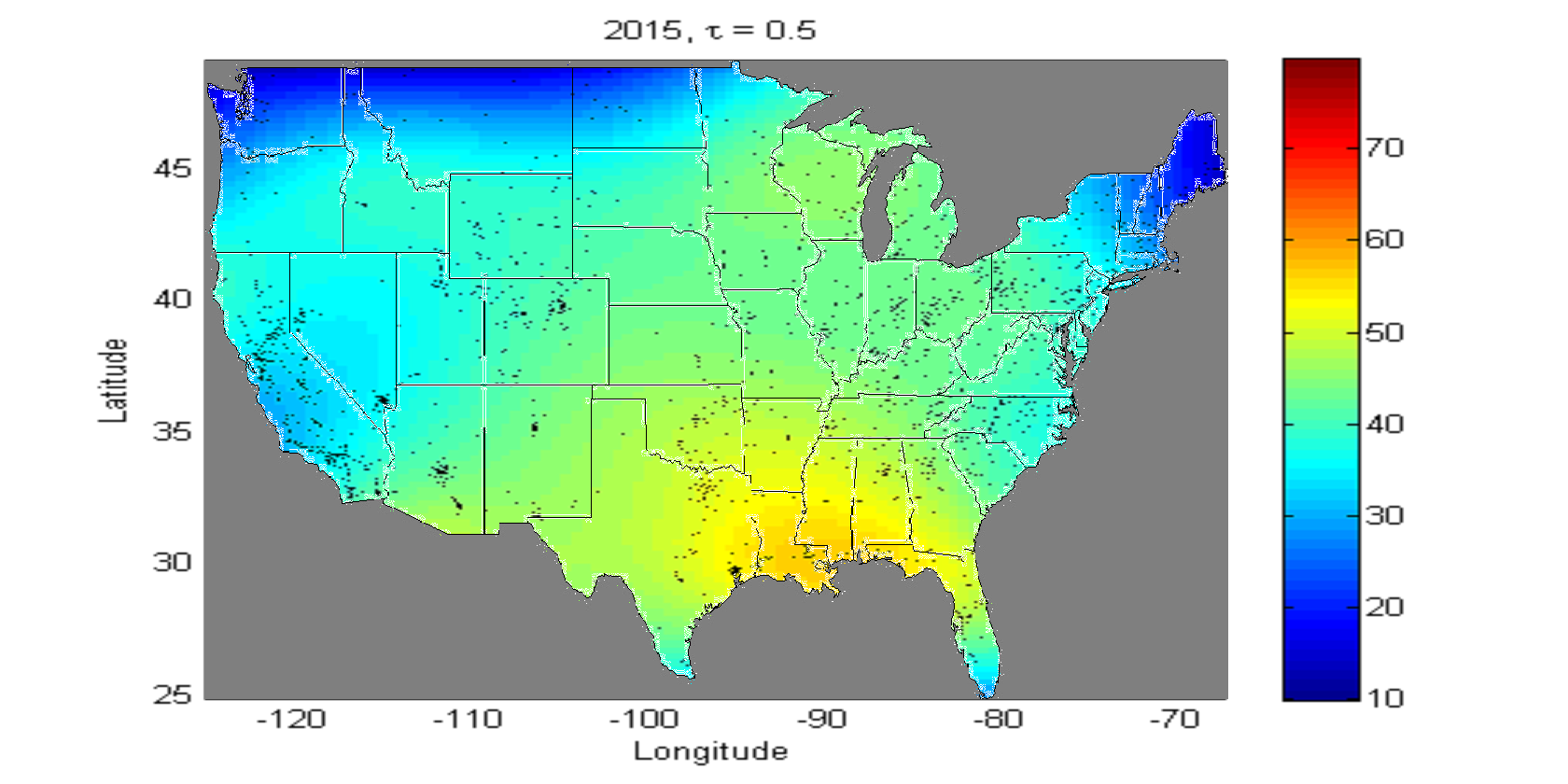
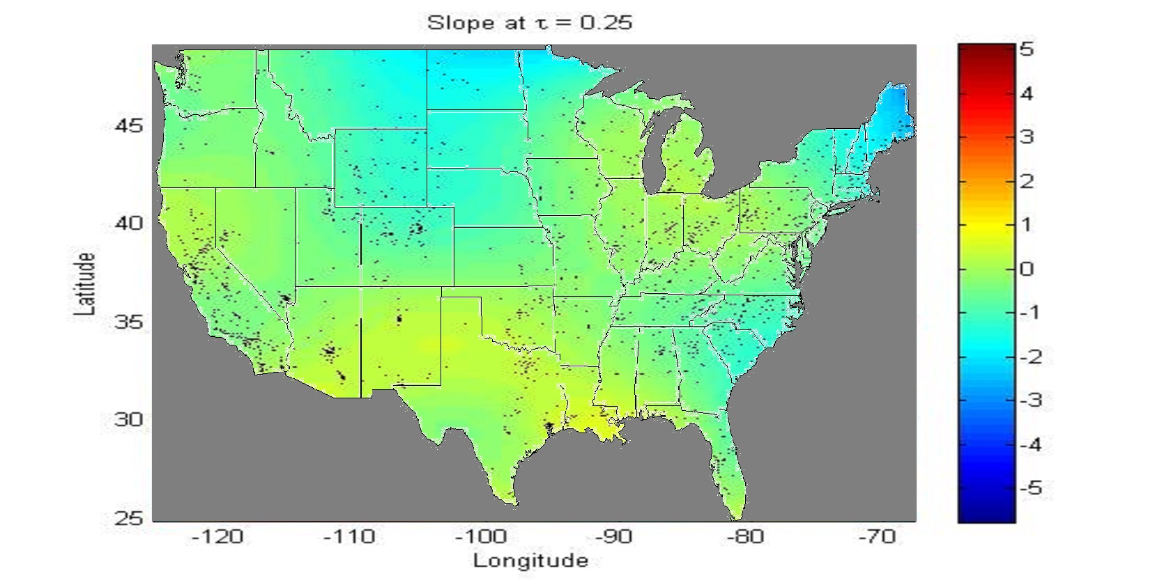
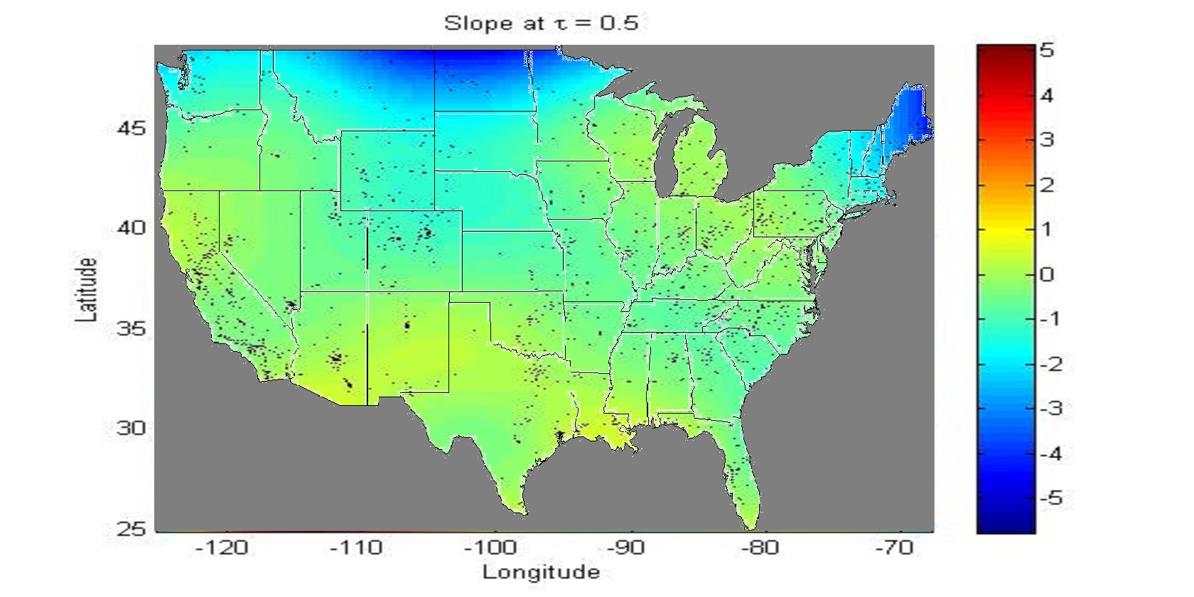
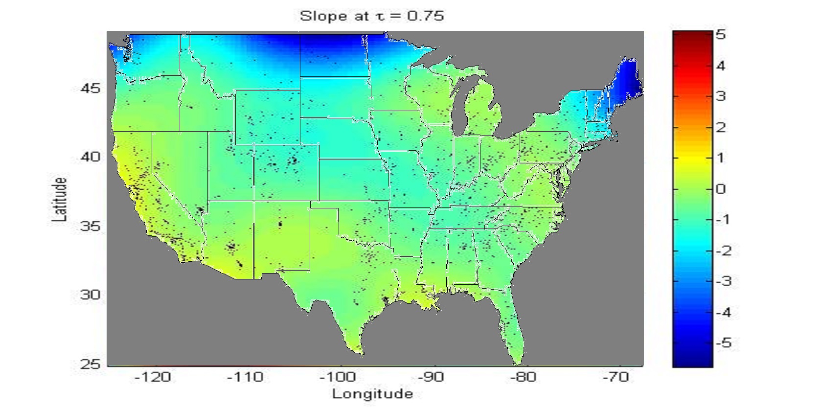
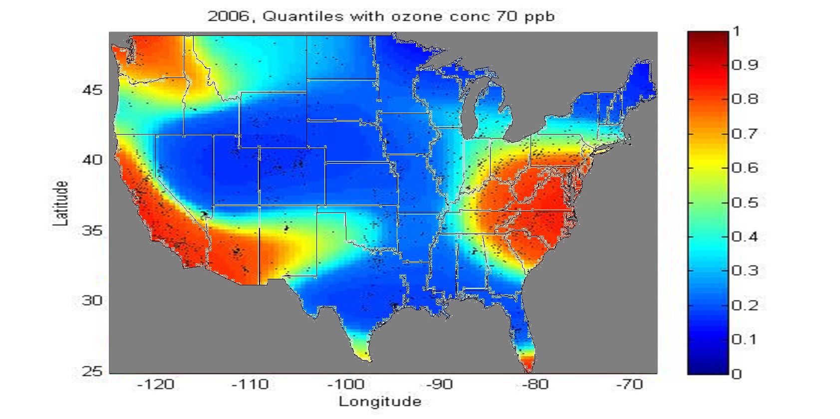
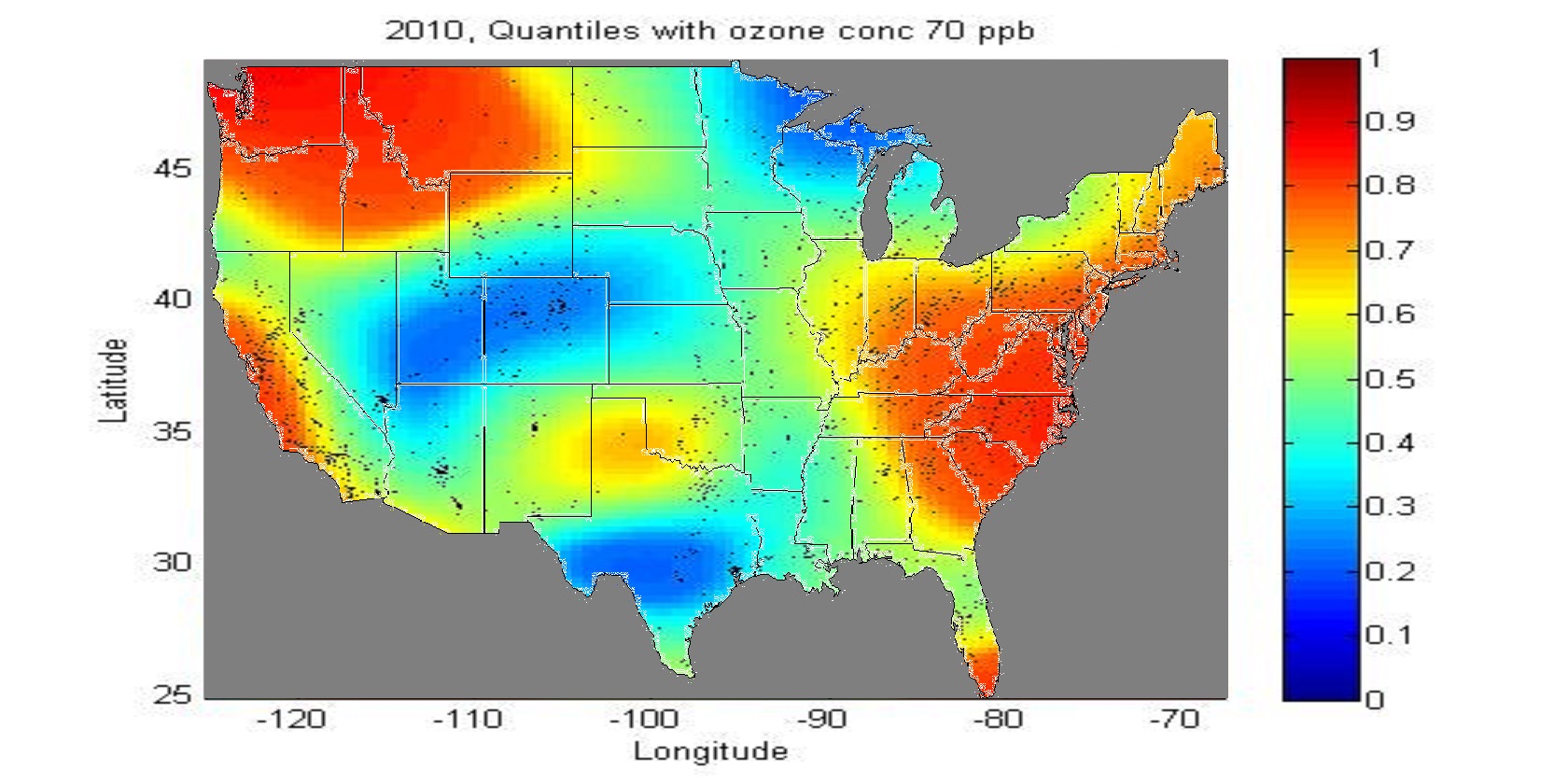
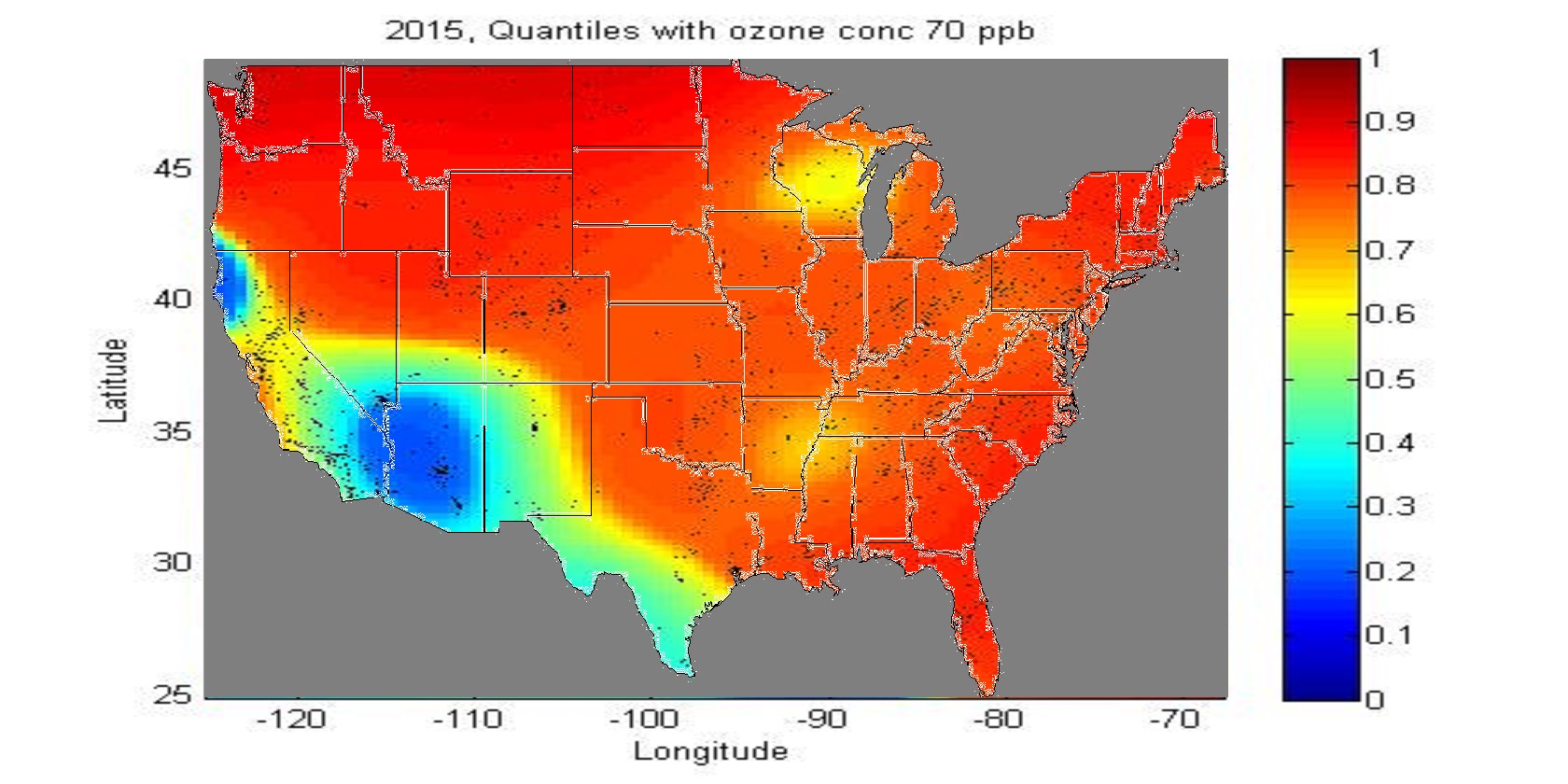
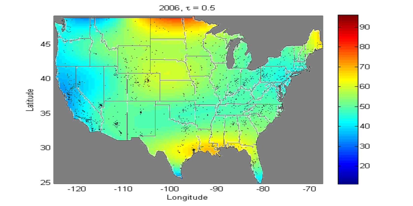
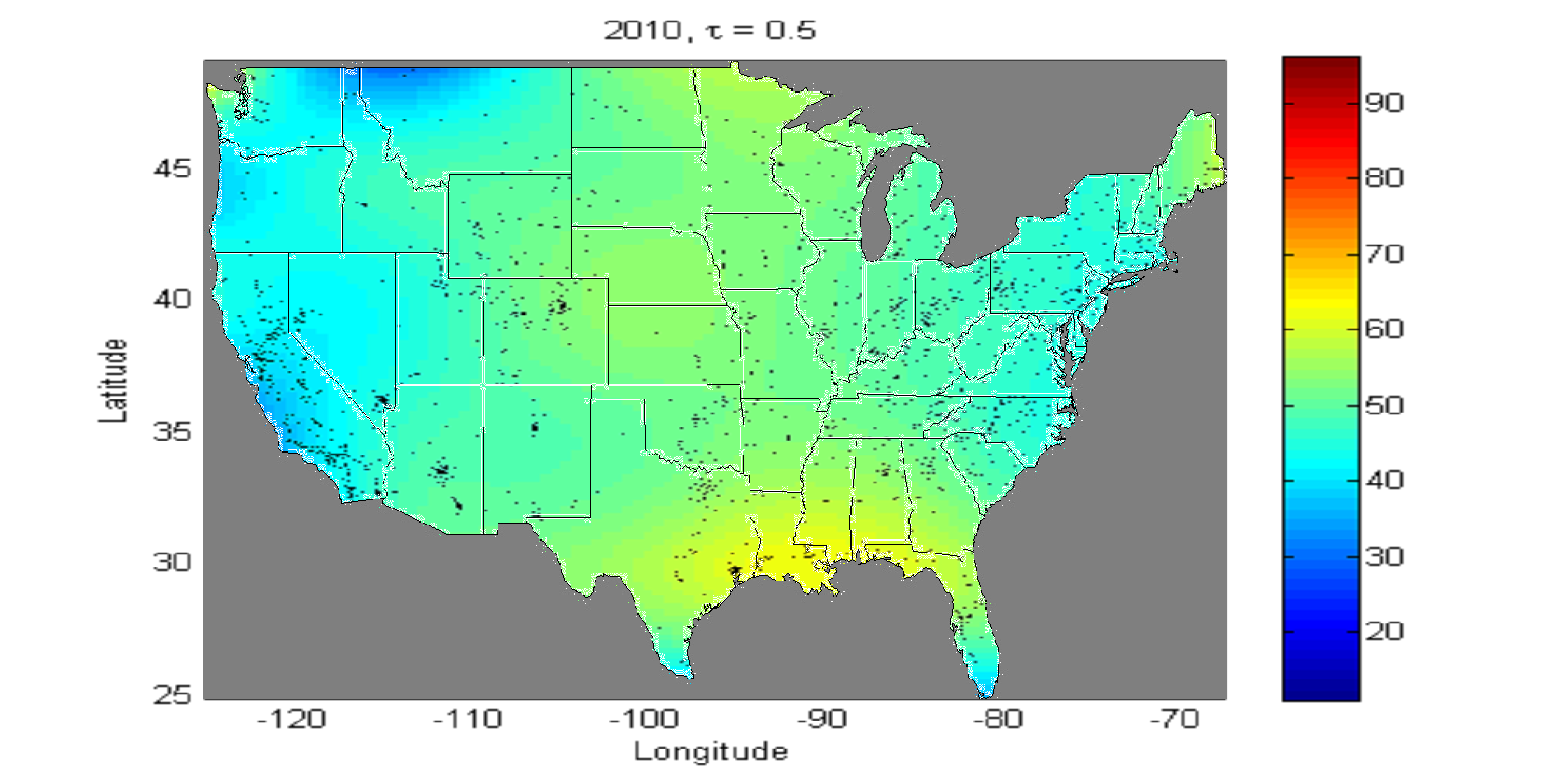
For the years 2006, 2010 and 2015 the daily 1-hour maximum and 8-hour maximum average ozone concentration are plotted over the US at the median level. It is noted that in the most of the parts of the US the daily 1-hour maximum average ozone concentration has decreased over time. Specifically the decreasing trend of 1-hour concentration is noticeable in the West North Central, Upper Midwest, Northeast and southern part of the South climate regions (see Figure 1, 2). The daily 8-hour maximum average ozone concentration level also has an overall decreasing trend over the time period considered. The 8-hour concentration has decreased quite a bit in the upper Northwest and West North Central regions. Besides, it has also decreased in the Northeast, South and Southeast regions (see Figures 4, 5). In Figure 6 we also show the quantile levels across the US where the 4th highest daily 8-hour maximum ozone concentration is 70 ppb. It is noted that over the last ten years the 4th highest daily 8-hour maximum ozone concentration in the US has generally a decreasing trend since 70 ppb ozone concentration is attained at relatively higher quantiles in the latter years.
Refer to caption
(a) Year : 2006,Ο„=0.52006𝜏0.52006,\tau=0.5
Refer to caption
(b) Year : 2010,Ο„=0.52010𝜏0.52010,\tau=0.5
Refer to caption
(c) Year : 2015,Ο„=0.52015𝜏0.52015,\tau=0.5
Figure 2: Daily 1-hour maximum average ozone concentration (in ppb) of the US in 2006, 2010 and 2015 at Ο„=0.5𝜏0.5\tau=0.5. The dots denote weather stations where data have been collected.
Refer to caption
(a) Slope at Ο„=0.25𝜏0.25\tau=0.25
Refer to caption
(b) Slope at Ο„=0.5𝜏0.5\tau=0.5
Refer to caption
(c) Slope at Ο„=0.75𝜏0.75\tau=0.75
Figure 3: Yearly rate of change of daily 1-hour maximum average ozone concentration (in ppb/year) of the US at Ο„=0.25,0.5,0.75𝜏0.250.50.75\tau=0.25,0.5,0.75. The dots denote weather stations where data have been collected.
Refer to caption
(a) Year : 2006,Ο„=0.52006𝜏0.52006,\tau=0.5
Refer to caption
(b) Year : 2010,Ο„=0.52010𝜏0.52010,\tau=0.5
Refer to caption
(c) Year : 2015,Ο„=0.52015𝜏0.52015,\tau=0.5
Figure 4: Daily 8-hour maximum average ozone concentration (in ppb) of the US in 2006, 2010 and 2015 at Ο„=0.5𝜏0.5\tau=0.5. The dots denote weather stations where data have been collected.
Refer to caption
(a) Slope at Ο„=0.25𝜏0.25\tau=0.25
Refer to caption
(b) Slope at Ο„=0.5𝜏0.5\tau=0.5
Refer to caption
(c) Slope at Ο„=0.75𝜏0.75\tau=0.75
Figure 5: Yearly rate of change of daily 8-hour maximum average ozone concentration (in ppb/year) of the US at Ο„=0.25,0.5,0.75𝜏0.250.50.75\tau=0.25,0.5,0.75. The dots denote weather stations where data have been collected.
Refer to caption
(a) 2006, quantiles at 4th highest 8-hr max ozone conc. 70 ppb
Refer to caption
(b) 2010, quantiles at 4th highest 8-hr max ozone conc. 70 ppb
Refer to caption
(c) 2015, quantiles at 4th highest 8-hr max ozone conc. 70 ppb
Figure 6: Quantiles at which 4th highest daily 8-hour maximum ozone concentration (in ppb) of the US is 70 ppb in 2006, 2010 and 2015.

6 Analysis of ozone concentration data of California

As mentioned in Barboza (2015), California has the worst smog in the US and it does not meet the existing smog limits. It also says that the air quality is the worst in the inland valleys, where pollution from vehicles and factories yields ozone in the presence of sunlight and that ozone is blown and trapped against the mountains. Some of the areas in California are so polluted that as per EPA, they are expected to meet the standards only by 2037, needing 12 more years to recover unlike the rest of the nation. According to the state Air Resources Board, about one-third population of California live in communities where the pollution level exceeds federal standards. As mentioned in the California Environmental Protection Agency site555Sourcehttps://www.arb.ca.gov/research/aaqs/caaqs/ozone/ozone.htm, in April 2005, the Air Resources Board retained the previous 1-hour ozone standard of 90 ppb and set a new 8-hour standard of 70 ppb. This ozone standard review was also mandated by the Children’s Environmental Health Protection Act.
Refer to caption
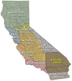
Figure 7: Region-wise division of California.
Refer to caption
(a) Year : 2006,Ο„=0.52006𝜏0.52006,\tau=0.5
Refer to caption
(b) Year : 2010,Ο„=0.52010𝜏0.52010,\tau=0.5
Refer to caption
(c) Year : 2015,Ο„=0.52015𝜏0.52015,\tau=0.5
Refer to caption
(d) Slope at Ο„=0.25𝜏0.25\tau=0.25
Refer to caption
(e) Slope at Ο„=0.5𝜏0.5\tau=0.5
Refer to caption
(f) Slope at Ο„=0.75𝜏0.75\tau=0.75
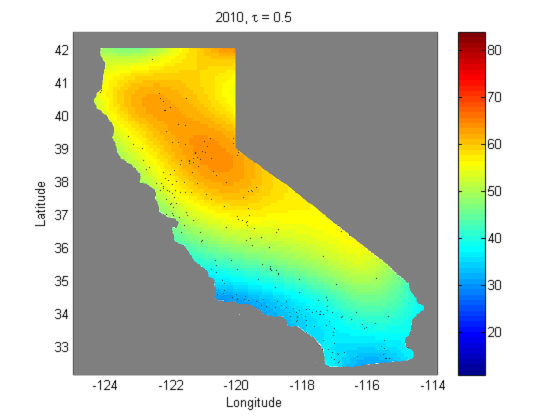
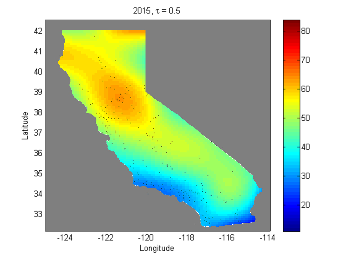
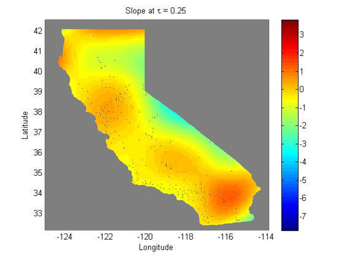
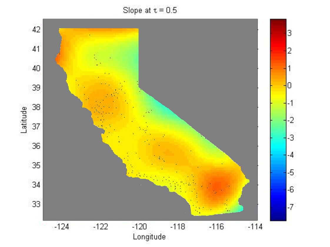
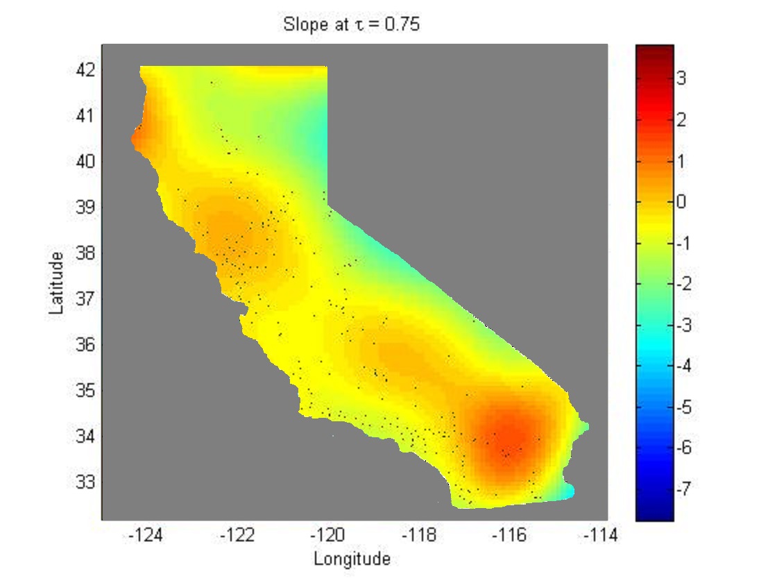
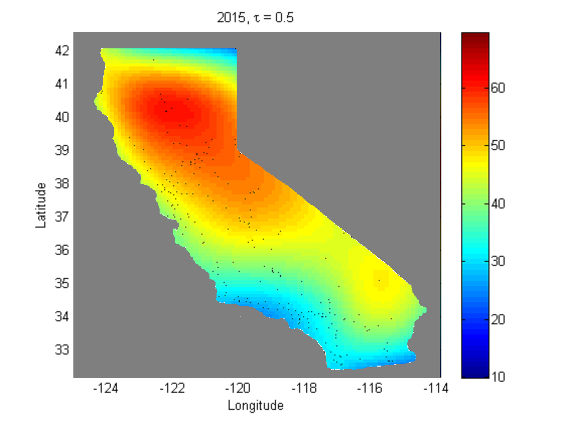
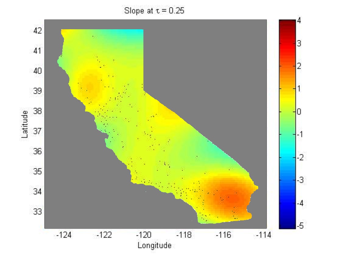
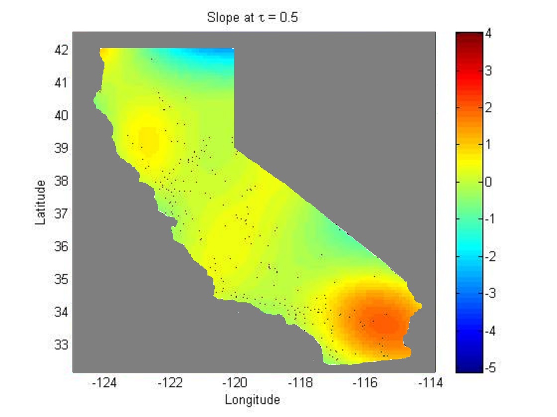
Figure 8: (a-c) Daily 1-hour maximum average ozone concentration (in ppb) of California in 2006, 2010 and 2015 at Ο„=0.5𝜏0.5\tau=0.5. (d-f) Yearly rate of change of daily 1-hour maximum average ozone concentration (in ppb/year) of California at Ο„=0.25,0.5,0.75𝜏0.250.50.75\tau=0.25,0.5,0.75.The dots denote weather stations where data have been collected.

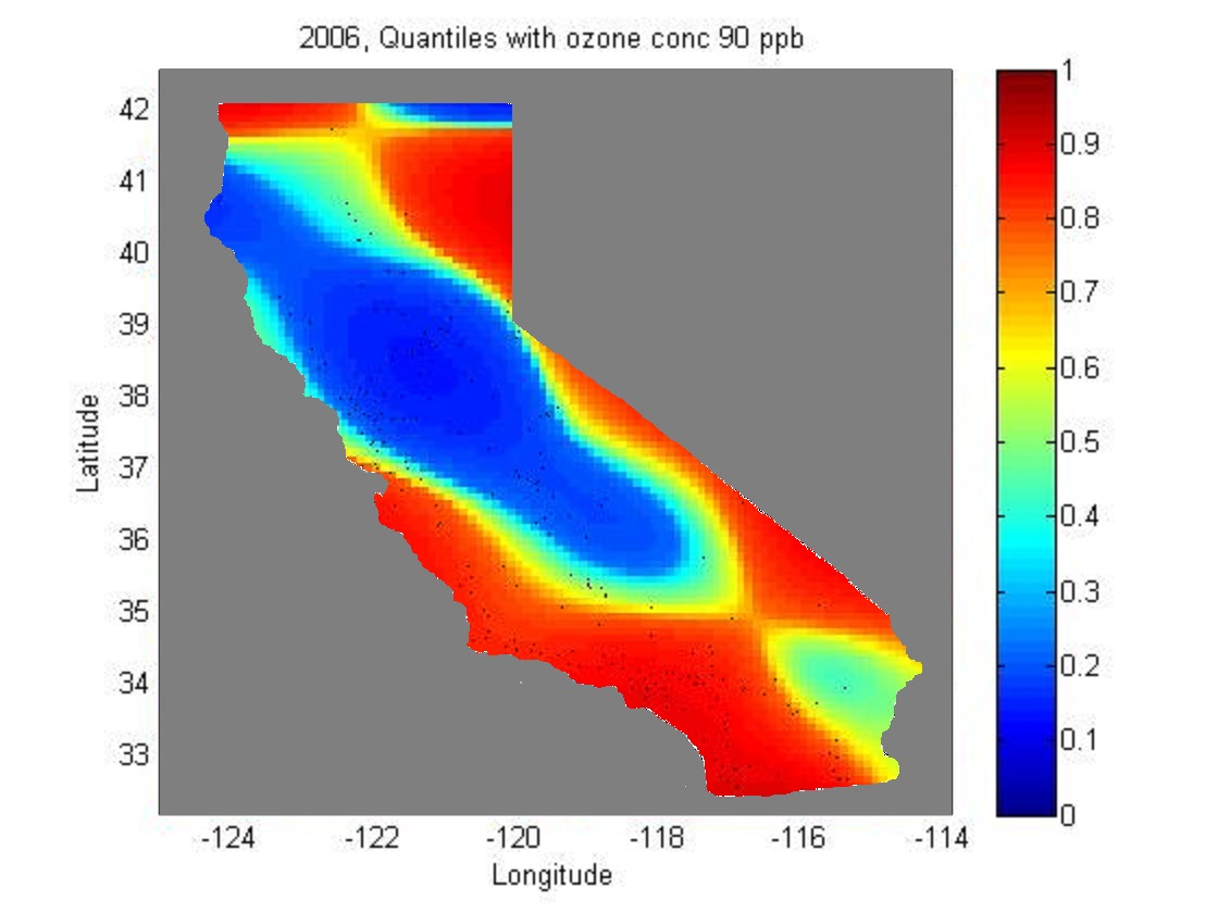
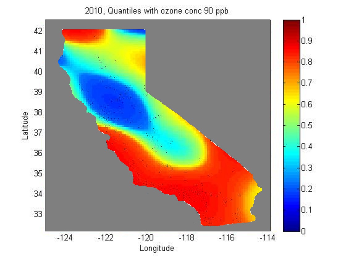
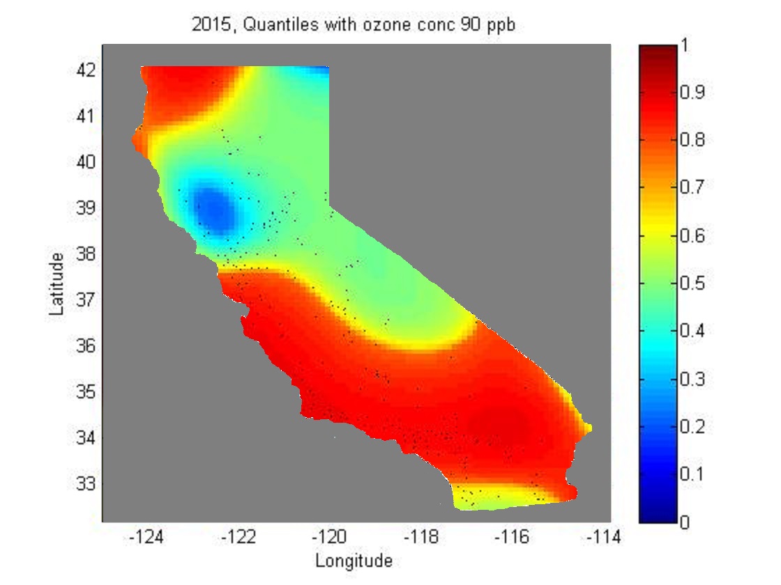
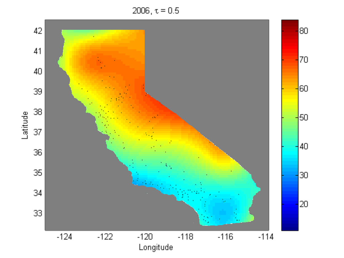
In this section, the spatio-temporal trend of daily 1-hour maximum and 8-hour maximum average ozone concentration data of California are analyzed over the time period 2006-2015 and spatial plots are shown for the years 2006, 2010 and 2015 at 505050-th quantile level. For those three years, we also show the quantile levels across California where the 4th highest daily 8-hour maximum ozone concentration is 70 ppb and 4th highest daily 1-hour maximum ozone concentration is 90 ppb. Similar to the previous section, the SSTQR (Bayes) method is used for the analysis and SSTQR (ML) estimate is used as the starting point of the MCMC chain. In this case also 10000 iterations are performed and the first 1000 iterations are disregarded as burn-in. It is noted that overall there is a decreasing trend of daily 1-hour maximum average concentration level at both the quantile levels considered. Specifically in the Northern California, Sacramento Region, Central Valley, High Sierra Desert, Los Angeles and San Diego (see Figures 7, 8) the 1-hour maximum average ozone concentration has noticeably decreased over time. It is also noted that in the Inland Empire region, it has a slightly increasing trend over time. As mentioned earlier, unlike in other parts of the US, Air Resources Board retained 1-hour ozone standard in California and its 8-hour standard has been 70 ppb for the last ten years while till September 2015, 8-hour standard for the rest of the country has been greater than or equal to 75 ppm. Thus to comply with the stricter rules, tighter controls on factories, vehicles, power plants and other emitters of smog-forming pollutants, the overall daily 1-hour maximum average ozone concentration of California shows a decreasing trend.
Refer to caption
(a) Year : 2006,Ο„=0.52006𝜏0.52006,\tau=0.5
Refer to caption
(b) Year : 2010,Ο„=0.52010𝜏0.52010,\tau=0.5
Refer to caption
(c) Year : 2015,Ο„=0.52015𝜏0.52015,\tau=0.5
Refer to caption
(d) Slope at Ο„=0.25𝜏0.25\tau=0.25
Refer to caption
(e) Slope at Ο„=0.5𝜏0.5\tau=0.5
Refer to caption
(f) Slope at Ο„=0.75𝜏0.75\tau=0.75
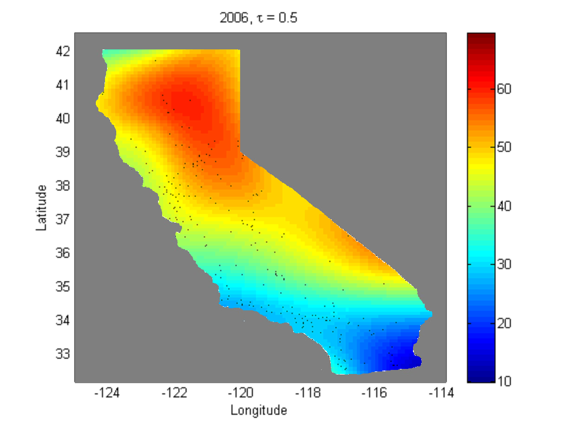
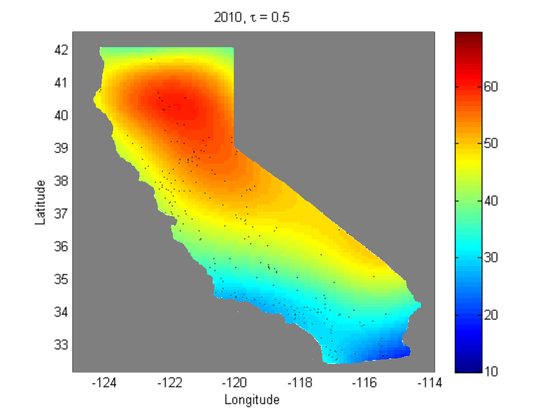
Figure 9: (a-c) Daily 8-hour maximum average ozone concentration (in ppb) of California in 2006, 2010 and 2015 at Ο„=0.5𝜏0.5\tau=0.5. (d-f) Yearly rate of change of daily 8-hour maximum average ozone concentration (in ppb/year) of California at Ο„=0.25,0.5,0.75𝜏0.250.50.75\tau=0.25,0.5,0.75.The dots denote weather stations where data have been collected.

The change in daily 8-hour maximum average ozone concentration varies a lot spatially over the time and there no particular temporal trend is observed for California as whole (see Figure 9). In the High Sierra Desert and north-east part of Northern California, the 8-hour maximum average ozone concentration has a decreasing trend over time at both the quantiles. On the other hand, in Sacramento Region, Inland Empire and San Diego, it has an increasing trend over the time. Not much temporal variations have been observed in the Bay Area and the Central Coast for both 1-hour maximum and 8-hour maximum average ozone concentration levels. In High Sierra Desert and Inland Empire, this ozone concentration level is changing rapidly.
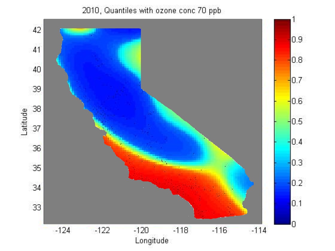
Refer to caption
(a) 2006, quantiles at 4th highest 8-hr max ozone conc. 70 ppb
Refer to caption
(b) 2010, quantiles at 4th highest 8-hr max ozone conc. 70 ppb
Refer to caption
(c) 2015, quantiles at 4th highest 8-hr max ozone conc. 70 ppb
Refer to caption
(d) 2006, quantiles at 4th highest 1-hr max ozone conc. 90 ppb
Refer to caption
(e) 2010, quantiles at 4th highest 1-hr max ozone conc. 90 ppb
Refer to caption
(f) 2015, quantiles at 4th highest 1-hr max ozone conc. 90 ppb
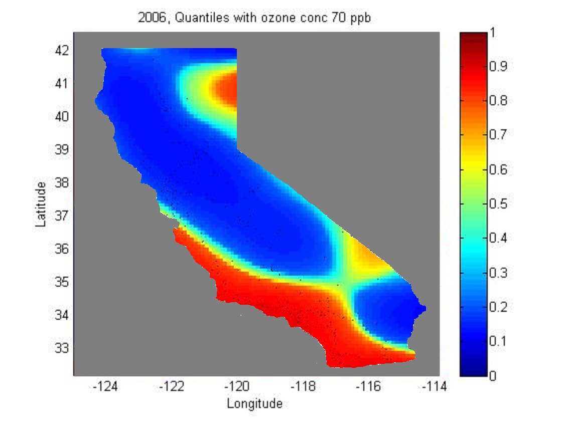
Figure 10: (a-c) Quantiles at which 4th highest daily 8-hour maximum ozone concentration (in ppb) of California is 70 ppb in 2006, 2010 and 2015. (d-f) Quantiles at which 4th highest daily 1-hour maximum ozone concentration (in ppb) of California is 90 ppb in 2006, 2010 and 2015.

In Figures 10(a), 10(b) and 10(c) it is noted that in Northern California, Bay Area, Sacramento Region and in the upper part of the Central Valley, the 4th highest daily 8-hour maximum ozone concentration threshold, i.e., 70 ppb is achieved at very lower quantile levels. In Los Angeles and San Diego area this threshold value is achieved at a higher quantile level. In Figures 10(d), 10(e) and 10(f) we note that at the junction of Bay Area, Sacramento Region, south Northern California and upper Central Valley the 4th highest daily 1-hour maximum ozone concentration threshold, i.e., 90 ppb is achieved at a lower quantile level compared to other parts of California. It is also noted that with time, the ozone concentration is decreasing in this region. In southern part of California, the threshold of daily 1-hour maximum ozone concentration is met at higher quantile level indicating that southern California is performing better in maintaining the ozone concentration level below recommended threshold level. But in San Diego area a strictly increasing pattern of ozone concentration is noted.

7 Discussion

As long as spatio-temporal regression is concerned, one of the major issues is the presence of missing temporal data at some locations. One way to solve this problem is to replace the missing data by estimated value based on the available data. It makes more sense to fit the model on the available data without using extrapolation or estimated missing values of data. In our regression model, the number of time-points of available data at various sites can be different (see equation (9)). This problem does not arise in the proposed method.

When the sample size is small at a location, in the method of Reich (2012), the estimated separate temporal quantile regression curve at that location will be widely affected by sampling fluctuations. If a lot of temporal data are missing at some locations, or when our data size is available only at a few temporal points, in spite of fitting separate quantile curves for all sites, it is desirable to fit a quantile curve considering the available data of all the sites together. Thus, estimation at the neighborhood of the locations with small temporal data can be improved by borrowing strength from neighboring sites. Hence the proposed method yields better estimates and is less affected by missing data and scarcity often.

In some approaches to spatio-temporal regression and time-series analysis, the temporal data are required to be obtained periodically. However in the proposed method, the temporal data are not required to be periodic. Thus we conclude that the proposed approach gives a natural Bayesian method for estimation and uncertainty quantification for simultaneous spatial quantile regression. The proposed method allows the data to be flexible with respect to missingness, monotonicity and low-sample size at individual locations. The method improves the quality of the inference by borrowing strength across all locations and all quantile levels by incorporating a natural non-parametric smoothing in its prior construction. By using B-spline functions in its smoothing, the method allows a relatively more efficient approach to likelihood evaluation compared with an analogous procedure based on Gaussian procedures.

As mentioned in Barboza (2015), according to the EPA ozone level has decreased by about one-third over the US since 1980 by imposing regulations targeting emissions from cars, factories, consumer products and other sources of pollutants. In this analysis, it is observed that overall there is a decreasing trend in the daily 1-hour and 8-hour maximum average ozone concentration levels in the US during the period 2006-2015. Specifically, in the lest ten years, the ozone concentration has decreased considerably in the northern part of the US. In California, it is noted that there is an overall decreasing trend in the 1-hour concentration while there is no specific trend for the 8-hour concentration and the trend varies a lot spatially. According to Barboza (2015), except for a few places in California, the rest of the US is expected to comply with the EPA ozone standards by 2025. Some of the most polluted areas in Southern California and the San Joaquin Valley are expected to comply with it by 2037.

Acknowledgements

This project was partially supported by NSF grant number DMS 1510238.

References

  • Barboza (2015) Barboza T. 2015. New attack on California’s dirty air, Los Angeles Times, Available at http://www.latimes.com/local/lanow/la-me-ln-what-new-smog-rules-mean-for-california-air-pollution-20150930-story.html.
  • Bethke (1980) Bethke A. 1980. Genetic algorithms as function optimizers, Available at https://deepblue.lib.umich.edu/handle/2027.42/3572.
  • Bondell etΒ al. (2010) Bondell HD, Reich RJ, Wang H. 2010. Non-crossing quantile regression curve estimation, Biometrika, 97: 825–838.
  • Chib and Greenberg (1995) Chib S, Greenberg E. 1995. Understanding the Metropolis-Hastings algorithm, The American Statistician, 49(4): 327–335.
  • Das (2016a) Das P. 2016. Black-box optimization on multiple simplex constrained blocks, arXiv:1609.02249v1.
  • Das (2016b) Das P. 2016. Derivative-free efficient global optimization of function of parameters from bounded intervals, arXiv:1604.08616v1.
  • Das (2016c) Das P. 2016. Derivative-free efficient global optimization on high-dimensional simplex, arXiv:1604.08636v1.
  • Das and Ghosal (2016) Das P, Ghosal S. 2016. Bayesian quantile regression using random B-spline series prior,Computational Statistics and Data Analysis (To appear, DOI : 10.1016/j.csda.2016.11.014) arXiv:1609.02950v1.
  • Boor (2001) Boor C. 2001. A Practical Guide to Splines, Revised Edition, New-York : Springer.
  • Dunson and Taylor (2005) Dunson DB, Taylor J. 2005. Approximate Bayesian inference for quantiles, Journal of Nonparametric Statistics, 17(3): 385–400.
  • Dunson and Park (2008) Dunson DB, Park J. 2008. Kernel stick-breaking processes, Biometrika, 95: 307–323.
  • Fraser (1957) Fraser A. 1957. Simulation of genetic systems by automatic digital computers, Australian Journal of Biological Sciences, 10: 484–491.
  • Gelfand and Kottas (2003) Gelfand AE, Kottas A. 2003. Bayesian semiparametric regression model for median residual life, Scandinavian Journal of Statistics, 30(4): 651–665.
  • Gelfand etΒ al. (2005) Gelfand AE, Kottas A, MacEachern SN. 2005. Bayesian non-parametric spatial modeling with Dirichlet process mixing, Journal of the American Statistical Association, 100: 1021–1035.
  • Goldberg (1989) Goldberg D. 1989. Genetic Algorithms in Search, Optimization and Machine Learning, Addison-Wesley Publishing Company.
  • Granville etΒ al. (1994) Granville V, Krivanek M, Rasson J. 1994. Simulated annealing: A proof of convergence, IEEE Transactions on Pattern Analysis and Machine Intelligence, 16: 652–656.
  • Griffin and Steel (2006) Griffin JE, Steel MFJ. 1994. Order-based dependent Dirichlet processes, Journal of the American Statistical Association, 101: 179–194.
  • He (1997) He X. 1997. Quantile curves without crossing, American Statistician, 51: 186–192.
  • Kirkpatrick etΒ al. (1983) Kirkpatrick S, Gelatt Jr C, Vecchi M. 1983. Optimization by Simulated Annealing, Australian Journal of Biological Sciences, 220: 671–680.
  • Koenkar (2005) Koenkar R. 2005. Quantile Regression, London: Cambridge University Press.
  • Koenkar and Bassett (1978) Koenkar R, Bassett G. 1978. Regression quantiles, Econometrica, 46: 33–50.
  • Kottas and Gelfand (2001) Kottas A, Gelfand A. 2001. Bayesian semiparametric median regression modeling, Journal of the American Statistical Association, 96: 1458–1468.
  • Kottas and Krnjajic (2009) Kottas A, Krnjajic M. 2009. Bayesian semiparametric modelling in quantile regression, Scandinavian Journal of Statistics, 36: 297–319.
  • Lee and Neocleous (2010) Lee D, Neocleous T. 2010. Bayesian quantile regression for count data with application to environmental epidemiology, Journal of the Royal Statistical Society: Series C, 59: 905–920.
  • Neocleous and Portnoy (2008) Neocleous T, Portnoy S. 2008. Quantile curves without crossing, Statistics and Probability Letters, 78: 1226–1229.
  • Oh etΒ al. (2011) Oh H, Lee T, Nychka D. 2011. Fast non-parametric quantile regression with arbitrary smoothing methods, Journal of Computational and Graphical Statistics, 20: 510–526.
  • Reich (2012) Reich BJ. 2012. Spatiotemporal quantile regression for detecting distributional changes in environmental processes, Journal of Royal Statistical Society Series C (Applied Statistics), 61(4): 535–553.
  • Reich and Fuentes (2007) Reich BJ, Fuentes M. 2007. A multivariate semiparametric Bayesian spatial modeling framework for hurricane surface wind fields, the Annals of Applied Statistics, 1: 249–264.
  • Reich etΒ al. (2011) Reich B, Fuentes M, Dunson D. 2011. Bayesian spatial quantile regression, Journal of the American Statistical Association, 106(493): 6–20.
  • Shim etΒ al. (2009) Shim J, Hwang C, Seok K. 2009. Non-crossing quantile regression via doubly penalized kernel machine, Computational Statistics, 24: 83–94.
  • Shim and Lee (2010) Shim J, Lee J. 2010. Restricted support vector quantile regression without crossing, Journal of the Korean Data and Information Science Society, 21(6): 1319–1325.
  • Sobotka and Kneib (2012) Sobotka F, Kneib T. 2012. Geoadditive expectile regression, Computational Statistics and Data Analysis, 56(4): 755–767.
  • Takeuchi (2004) Takeuchi I. 2004. Non-crossing quantile regression curves by support vector and its effcient implementation, Proceedings of 2004 IEEE IJCNN, 1: 401–406.
  • Takeuchi etΒ al. (2006) Takeuchi T, Le Q, Sears T, Smola AJ. 2006. Noparametric quantile estimation, Journal of Machine Learning Research, 7: 1231–1264.
  • Tokdar and Kadane (2012) Tokdar S, Kadane JB. 2012. Simultaneous linear quantile regression : a semiparametric Bayesian approach, Bayesian Analysis, 7(1): 51–72.
  • Vapnik (1995) Vapnik V. 1995. The Nature of Statistical Learning Theory, New York: Springler-Verlag.
  • Wu and Liu (2009) Wu Y, Liu Y. 2009. Stepwise multiple quantile regression estimation using non-crossing constraints, Statistics and Its Inference, 2: 299–310.
  • Yu and Moyeed (2001) Yu K, Moyeed RA. 2001. Bayesian quantile regression, Statistics and Probability Letters, 54: 437–447.

Appendix A Likelihood computation

Recall, 0=t0<t1<β‹―<tp1=10subscript𝑑0subscript𝑑1β‹―subscript𝑑subscript𝑝110=t_{0}<t_{1}<\cdots<t_{p_{1}}=1 are the equidistant knots on the interval [0,1]01[0,1] such that tiβˆ’tiβˆ’1=1/p1subscript𝑑𝑖subscript𝑑𝑖11subscript𝑝1t_{i}-t_{i-1}=1/p_{1} for i=1,…,p1𝑖1…subscript𝑝1i=1,\ldots,p_{1} and {Bj,m1​(β‹…)}j=1p1+m1superscriptsubscriptsubscript𝐡𝑗subscriptπ‘š1⋅𝑗1subscript𝑝1subscriptπ‘š1\{B_{j,m_{1}}(\cdot)\}_{j=1}^{p_{1}+m_{1}} are the basis functions of B-splines of degree m1subscriptπ‘š1m_{1} on [0,1]01[0,1] on the above-mentioned equidistant knots. Then Equation (4) can be written as

Q(Ο„|\displaystyle Q(\tau| x,𝐳)\displaystyle x,\mathbf{z})
=x​ξ1​(Ο„,𝐳)+(1βˆ’x)​ξ2​(Ο„,𝐳)absentπ‘₯subscriptπœ‰1𝜏𝐳1π‘₯subscriptπœ‰2𝜏𝐳\displaystyle=x\xi_{1}(\tau,\mathbf{z})+(1-x)\xi_{2}(\tau,\mathbf{z})
=xβ€‹βˆ‘j=1p1+m1ΞΈj​(𝐳)​Bj,m1​(Ο„)+(1βˆ’x)β€‹βˆ‘j=1p1+m1Ο•j​(𝐳)​Bj,m1​(Ο„)absentπ‘₯superscriptsubscript𝑗1subscript𝑝1subscriptπ‘š1subscriptπœƒπ‘—π³subscript𝐡𝑗subscriptπ‘š1𝜏1π‘₯superscriptsubscript𝑗1subscript𝑝1subscriptπ‘š1subscriptitalic-ϕ𝑗𝐳subscript𝐡𝑗subscriptπ‘š1𝜏\displaystyle=x\sum_{j=1}^{p_{1}+m_{1}}\theta_{j}(\mathbf{z})B_{j,m_{1}}(\tau)+(1-x)\sum_{j=1}^{p_{1}+m_{1}}\phi_{j}(\mathbf{z})B_{j,m_{1}}(\tau)
=xβ€‹βˆ‘j=1p1+m1Bj,m1​(Ο„)β€‹βˆ‘k1=1p2+m2β€¦β€‹βˆ‘kd=1p2+m2Ξ±j​k1​⋯​kd​Bk1,m2​(z1)​⋯​Bkd,m2​(zd)absentπ‘₯superscriptsubscript𝑗1subscript𝑝1subscriptπ‘š1subscript𝐡𝑗subscriptπ‘š1𝜏superscriptsubscriptsubscriptπ‘˜11subscript𝑝2subscriptπ‘š2…superscriptsubscriptsubscriptπ‘˜π‘‘1subscript𝑝2subscriptπ‘š2subscript𝛼𝑗subscriptπ‘˜1β‹―subscriptπ‘˜π‘‘subscript𝐡subscriptπ‘˜1subscriptπ‘š2subscript𝑧1β‹―subscript𝐡subscriptπ‘˜π‘‘subscriptπ‘š2subscript𝑧𝑑\displaystyle=x\sum_{j=1}^{p_{1}+m_{1}}B_{j,m_{1}}(\tau)\sum_{k_{1}=1}^{p_{2}+m_{2}}\ldots\sum_{k_{d}=1}^{p_{2}+m_{2}}\alpha_{jk_{1}\cdots k_{d}}B_{k_{1},m_{2}}(z_{1})\cdots B_{k_{d},m_{2}}(z_{d})
+(1βˆ’x)β€‹βˆ‘j=1p1+m1Bj,m1​(Ο„)β€‹βˆ‘k1=1p2+m2β€¦β€‹βˆ‘kd=1p2+m2Ξ²j​k1​⋯​kd​Bk1,m2​(z1)​⋯​Bkd,m2​(zd)1π‘₯superscriptsubscript𝑗1subscript𝑝1subscriptπ‘š1subscript𝐡𝑗subscriptπ‘š1𝜏superscriptsubscriptsubscriptπ‘˜11subscript𝑝2subscriptπ‘š2…superscriptsubscriptsubscriptπ‘˜π‘‘1subscript𝑝2subscriptπ‘š2subscript𝛽𝑗subscriptπ‘˜1β‹―subscriptπ‘˜π‘‘subscript𝐡subscriptπ‘˜1subscriptπ‘š2subscript𝑧1β‹―subscript𝐡subscriptπ‘˜π‘‘subscriptπ‘š2subscript𝑧𝑑\displaystyle+(1-x)\sum_{j=1}^{p_{1}+m_{1}}B_{j,m_{1}}(\tau)\sum_{k_{1}=1}^{p_{2}+m_{2}}\ldots\sum_{k_{d}=1}^{p_{2}+m_{2}}\beta_{jk_{1}\cdots k_{d}}B_{k_{1},m_{2}}(z_{1})\cdots B_{k_{d},m_{2}}(z_{d}) (14)

We evaluate the likelihood by a similar approach of Tokdar and Kadane (2012) and Das and Ghosal (2016). Suppose that we have data for L𝐿L spatial sites z1,…,zLsubscript𝑧1…subscript𝑧𝐿z_{1},\ldots,z_{L} and at the l𝑙l-th site, {Xl​i,Yl​i}i=1nlsuperscriptsubscriptsubscript𝑋𝑙𝑖subscriptπ‘Œπ‘™π‘–π‘–1subscript𝑛𝑙\{X_{li},Y_{li}\}_{i=1}^{n_{l}} denote the values of the explanatory variable (time) and the response variable, nlsubscript𝑛𝑙n_{l} being the number of data-points for l=1,…,L𝑙1…𝐿l=1,\ldots,L, the likelihood is given by ∏l=1L{∏i=1nlf​(Yl​i|Xl​i,𝐳l)}superscriptsubscriptproduct𝑙1𝐿superscriptsubscriptproduct𝑖1subscript𝑛𝑙𝑓conditionalsubscriptπ‘Œπ‘™π‘–subscript𝑋𝑙𝑖subscript𝐳𝑙\prod_{l=1}^{L}\bigg{\{}\prod_{i=1}^{n_{l}}f(Y_{li}|X_{li},\mathbf{z}_{l})\bigg{\}} where

f​(Yl​i|Xl​i,𝐳l)=(βˆ‚βˆ‚Ο„β€‹Q​(Ο„|Xl​i,𝐳l)|Ο„=Ο„X​(Yl​i,𝐳l))βˆ’1,l=1,…,L,i=1,…,nl.formulae-sequence𝑓conditionalsubscriptπ‘Œπ‘™π‘–subscript𝑋𝑙𝑖subscript𝐳𝑙superscriptevaluated-atπœπ‘„conditional𝜏subscript𝑋𝑙𝑖subscriptπ³π‘™πœsubscriptπœπ‘‹subscriptπ‘Œπ‘™π‘–subscript𝐳𝑙1formulae-sequence𝑙1…𝐿𝑖1…subscript𝑛𝑙\displaystyle f(Y_{li}|X_{li},\mathbf{z}_{l})=\bigg{(}\frac{\partial}{\partial\tau}Q(\tau|X_{li},\mathbf{z}_{l})\bigg{|}_{\tau=\tau_{X}(Y_{li},\mathbf{z}_{l})}\bigg{)}^{-1},\;l=1,\ldots,L,\;i=1,\ldots,n_{l}.

Now,

log⁑f​(Yl​i|Xl​i,𝐳l)=𝑓conditionalsubscriptπ‘Œπ‘™π‘–subscript𝑋𝑙𝑖subscript𝐳𝑙absent\displaystyle\log f(Y_{li}|X_{li},\mathbf{z}_{l})= βˆ’log⁑(βˆ‚βˆ‚Ο„β€‹Q​(Ο„|Xl​i,𝐳l)|Ο„=Ο„Xl​i​(Yl​i,𝐳l))evaluated-atπœπ‘„conditional𝜏subscript𝑋𝑙𝑖subscriptπ³π‘™πœsubscript𝜏subscript𝑋𝑙𝑖subscriptπ‘Œπ‘™π‘–subscript𝐳𝑙\displaystyle-\log\bigg{(}\frac{\partial}{\partial\tau}Q(\tau|X_{li},\mathbf{z}_{l})\bigg{|}_{\tau=\tau_{X_{li}}(Y_{li},\mathbf{z}_{l})}\bigg{)}
=\displaystyle= βˆ’log⁑{Xl​iβ€‹βˆ‚βˆ‚Ο„β€‹ΞΎ1​(Ο„,𝐳l)+(1βˆ’Xl​i)β€‹βˆ‚βˆ‚Ο„β€‹ΞΎ2​(Ο„,𝐳l)}|Ο„=Ο„Xl​i​(Yl​i,𝐳l)evaluated-atsubscriptπ‘‹π‘™π‘–πœsubscriptπœ‰1𝜏subscript𝐳𝑙1subscriptπ‘‹π‘™π‘–πœsubscriptπœ‰2𝜏subscriptπ³π‘™πœsubscript𝜏subscript𝑋𝑙𝑖subscriptπ‘Œπ‘™π‘–subscript𝐳𝑙\displaystyle-\log\bigg{\{}X_{li}\frac{\partial}{\partial\tau}\xi_{1}(\tau,\mathbf{z}_{l})+(1-X_{li})\frac{\partial}{\partial\tau}\xi_{2}(\tau,\mathbf{z}_{l})\bigg{\}}\bigg{|}_{\tau=\tau_{X_{li}}(Y_{li},\mathbf{z}_{l})} (15)

where Ο„Xl​i​(Yl​i,𝐳l)subscript𝜏subscript𝑋𝑙𝑖subscriptπ‘Œπ‘™π‘–subscript𝐳𝑙\tau_{X_{li}}(Y_{li},\mathbf{z}_{l}) is the solution of

Yl​i=Xl​i​ξ1​(Ο„,𝐳l)+(1βˆ’Xl​i)​ξ2​(Ο„,𝐳l).subscriptπ‘Œπ‘™π‘–subscript𝑋𝑙𝑖subscriptπœ‰1𝜏subscript𝐳𝑙1subscript𝑋𝑙𝑖subscriptπœ‰2𝜏subscript𝐳𝑙\displaystyle Y_{li}=X_{li}\xi_{1}(\tau,\mathbf{z}_{l})+(1-X_{li})\xi_{2}(\tau,\mathbf{z}_{l}). (16)

For any given location 𝐙=𝐳𝐙𝐳\mathbf{Z}=\mathbf{z}, since ΞΎ1​(β‹…,𝐳)subscriptπœ‰1⋅𝐳\xi_{1}(\cdot,\mathbf{z}) and ΞΎ2​(β‹…,𝐳)subscriptπœ‰2⋅𝐳\xi_{2}(\cdot,\mathbf{z}) are strictly monotonic, their convex combination is also strictly monotonic. Hence there will exist a unique solution of equation (16). Using the properties of derivative of B-spline (Boor (2001)) we have

dd​t​ξ1​(t,𝐳)=dd​tβ€‹βˆ‘j=1p1+m1ΞΈj​(𝐳)​Bj,m1​(t)=βˆ‘j=2p1+m1ΞΈjβˆ—β€‹(𝐳)​Bjβˆ’1,m1βˆ’1​(t),𝑑𝑑𝑑subscriptπœ‰1𝑑𝐳𝑑𝑑𝑑superscriptsubscript𝑗1subscript𝑝1subscriptπ‘š1subscriptπœƒπ‘—π³subscript𝐡𝑗subscriptπ‘š1𝑑superscriptsubscript𝑗2subscript𝑝1subscriptπ‘š1subscriptsuperscriptπœƒπ‘—π³subscript𝐡𝑗1subscriptπ‘š11𝑑\displaystyle\frac{d}{dt}\xi_{1}(t,\mathbf{z})=\frac{d}{dt}\sum_{j=1}^{p_{1}+m_{1}}\theta_{j}(\mathbf{z})B_{j,m_{1}}(t)=\sum_{j=2}^{p_{1}+m_{1}}\theta^{*}_{j}(\mathbf{z})B_{j-1,m_{1}-1}(t),
dd​t​ξ2​(t,𝐳)=dd​tβ€‹βˆ‘j=1p1+m1Ο•j​(𝐳)​Bj,m1​(t)=βˆ‘j=2p1+m1Ο•jβˆ—β€‹(𝐳)​Bjβˆ’1,m1βˆ’1​(t),𝑑𝑑𝑑subscriptπœ‰2𝑑𝐳𝑑𝑑𝑑superscriptsubscript𝑗1subscript𝑝1subscriptπ‘š1subscriptitalic-ϕ𝑗𝐳subscript𝐡𝑗subscriptπ‘š1𝑑superscriptsubscript𝑗2subscript𝑝1subscriptπ‘š1subscriptsuperscriptitalic-ϕ𝑗𝐳subscript𝐡𝑗1subscriptπ‘š11𝑑\displaystyle\frac{d}{dt}\xi_{2}(t,\mathbf{z})=\frac{d}{dt}\sum_{j=1}^{p_{1}+m_{1}}\phi_{j}(\mathbf{z})B_{j,m_{1}}(t)=\sum_{j=2}^{p_{1}+m_{1}}\phi^{*}_{j}(\mathbf{z})B_{j-1,m_{1}-1}(t), (17)

where

ΞΈjβˆ—β€‹(𝐳)=(p1+m1)​(ΞΈj​(𝐳)βˆ’ΞΈjβˆ’1​(𝐳)),Ο•jβˆ—β€‹(𝐳)=(p1+m1)​(Ο•j​(𝐳)βˆ’Ο•jβˆ’1​(𝐳)),formulae-sequencesubscriptsuperscriptπœƒπ‘—π³subscript𝑝1subscriptπ‘š1subscriptπœƒπ‘—π³subscriptπœƒπ‘—1𝐳subscriptsuperscriptitalic-ϕ𝑗𝐳subscript𝑝1subscriptπ‘š1subscriptitalic-ϕ𝑗𝐳subscriptitalic-ϕ𝑗1𝐳\displaystyle\theta^{*}_{j}(\mathbf{z})=(p_{1}+m_{1})(\theta_{j}(\mathbf{z})-\theta_{j-1}(\mathbf{z})),\;\phi^{*}_{j}(\mathbf{z})=(p_{1}+m_{1})(\phi_{j}(\mathbf{z})-\phi_{j-1}(\mathbf{z})),

for j=2,…,p1+m1𝑗2…subscript𝑝1subscriptπ‘š1j=2,\ldots,p_{1}+m_{1}. Now, using equation (15) and (17), we have

log⁑f​(Yl​i|Xl​i,𝐳l)=𝑓conditionalsubscriptπ‘Œπ‘™π‘–subscript𝑋𝑙𝑖subscript𝐳𝑙absent\displaystyle\log f(Y_{li}|X_{li},\mathbf{z}_{l})= βˆ’log{Xl​iβˆ‘j=2p1+m1ΞΈjβˆ—(𝐳l)Bjβˆ’1,m1βˆ’1(Ο„Xl​i(Yl​i,𝐳l))\displaystyle-\log\bigg{\{}X_{li}\sum_{j=2}^{p_{1}+m_{1}}\theta^{*}_{j}(\mathbf{z}_{l})B_{j-1,m_{1}-1}(\tau_{X_{li}}(Y_{li},\mathbf{z}_{l}))
+(1βˆ’Xl​i)βˆ‘j=2p1+m1Ο•jβˆ—(𝐳l)Bjβˆ’1,m1βˆ’1(Ο„Xl​i(Yl​i,𝐳l))}.\displaystyle+(1-X_{li})\sum_{j=2}^{p_{1}+m_{1}}\phi^{*}_{j}(\mathbf{z}_{l})B_{j-1,m_{1}-1}(\tau_{X_{li}}(Y_{li},\mathbf{z}_{l}))\bigg{\}}. (18)

Hence the total log-likelihood is given by

βˆ‘l=1Lβˆ‘i=1nllog⁑f​(Yl​i|Xl​i,𝐳l)=superscriptsubscript𝑙1𝐿superscriptsubscript𝑖1subscript𝑛𝑙𝑓conditionalsubscriptπ‘Œπ‘™π‘–subscript𝑋𝑙𝑖subscript𝐳𝑙absent\displaystyle\sum_{l=1}^{L}\sum_{i=1}^{n_{l}}\log f(Y_{li}|X_{li},\mathbf{z}_{l})= βˆ’βˆ‘l=1Lβˆ‘i=1nllog{Xl​iβˆ‘j=2p1+m1ΞΈjβˆ—(𝐳l)Bjβˆ’1,m1βˆ’1(Ο„Xl​i(Yl​i,𝐳l))\displaystyle-\sum_{l=1}^{L}\sum_{i=1}^{n_{l}}\log\bigg{\{}X_{li}\sum_{j=2}^{p_{1}+m_{1}}\theta^{*}_{j}(\mathbf{z}_{l})B_{j-1,m_{1}-1}(\tau_{X_{li}}(Y_{li},\mathbf{z}_{l}))
+(1βˆ’Xl​i)βˆ‘j=2p1+m1Ο•jβˆ—(𝐳l)Bjβˆ’1,m1βˆ’1(Ο„Xl​i(Yl​i,𝐳l))}.\displaystyle+(1-X_{li})\sum_{j=2}^{p_{1}+m_{1}}\phi^{*}_{j}(\mathbf{z}_{l})B_{j-1,m_{1}-1}(\tau_{X_{li}}(Y_{li},\mathbf{z}_{l}))\bigg{\}}. (19)

We note that the parameters of the likelihood are the coefficients of the B-spline basis expansion of {ΞΈj​(𝐳)}j=1p1+m1superscriptsubscriptsubscriptπœƒπ‘—π³π‘—1subscript𝑝1subscriptπ‘š1\{\theta_{j}(\mathbf{z})\}_{j=1}^{p_{1}+m_{1}} and {Ο•j​(𝐳)}j=1p1+m1superscriptsubscriptsubscriptitalic-ϕ𝑗𝐳𝑗1subscript𝑝1subscriptπ‘š1\{\phi_{j}(\mathbf{z})\}_{j=1}^{p_{1}+m_{1}} which are

0=Ξ±1​k1​⋯​kd<β‹―<Ξ±(p1+m1)​k1​⋯​kd=1,0subscript𝛼1subscriptπ‘˜1β‹―subscriptπ‘˜π‘‘β‹―subscript𝛼subscript𝑝1subscriptπ‘š1subscriptπ‘˜1β‹―subscriptπ‘˜π‘‘1\displaystyle 0=\alpha_{1k_{1}\cdots k_{d}}<\cdots<\alpha_{(p_{1}+m_{1})k_{1}\cdots k_{d}}=1,
0=Ξ²1​k1​⋯​kd<β‹―<Ξ²(p1+m1)​k1​⋯​kd=1,0subscript𝛽1subscriptπ‘˜1β‹―subscriptπ‘˜π‘‘β‹―subscript𝛽subscript𝑝1subscriptπ‘š1subscriptπ‘˜1β‹―subscriptπ‘˜π‘‘1\displaystyle 0=\beta_{1k_{1}\cdots k_{d}}<\cdots<\beta_{(p_{1}+m_{1})k_{1}\cdots k_{d}}=1, (20)

for {k1,…,kd}∈{1,…,(p2+m2)}dsubscriptπ‘˜1…subscriptπ‘˜π‘‘superscript1…subscript𝑝2subscriptπ‘š2𝑑\{k_{1},\ldots,k_{d}\}\in\{1,\ldots,(p_{2}+m_{2})\}^{d}.

Appendix B Block Metropolis-Hastings MCMC algorithm

Recall that

Ξ³j​k1​⋯​kd=Ξ±(j+1)​k1​⋯​kdβˆ’Ξ±j​k1​⋯​kd,Ξ΄j​k1​⋯​kd=Ξ²(j+1)​k1​⋯​kdβˆ’Ξ²j​k1​⋯​kd,formulae-sequencesubscript𝛾𝑗subscriptπ‘˜1β‹―subscriptπ‘˜π‘‘subscript𝛼𝑗1subscriptπ‘˜1β‹―subscriptπ‘˜π‘‘subscript𝛼𝑗subscriptπ‘˜1β‹―subscriptπ‘˜π‘‘subscript𝛿𝑗subscriptπ‘˜1β‹―subscriptπ‘˜π‘‘subscript𝛽𝑗1subscriptπ‘˜1β‹―subscriptπ‘˜π‘‘subscript𝛽𝑗subscriptπ‘˜1β‹―subscriptπ‘˜π‘‘\displaystyle\gamma_{jk_{1}\cdots k_{d}}=\alpha_{(j+1)k_{1}\cdots k_{d}}-\alpha_{jk_{1}\cdots k_{d}},\;\delta_{jk_{1}\cdots k_{d}}=\beta_{(j+1)k_{1}\cdots k_{d}}-\beta_{jk_{1}\cdots k_{d}}, (21)

for j=1,…,p1+m1βˆ’1𝑗1…subscript𝑝1subscriptπ‘š11j=1,\ldots,p_{1}+m_{1}-1 and {k1,…,kd}∈{1,…,(p2+m2)}dsubscriptπ‘˜1…subscriptπ‘˜π‘‘superscript1…subscript𝑝2subscriptπ‘š2𝑑\{k_{1},\ldots,k_{d}\}\in\{1,\ldots,(p_{2}+m_{2})\}^{d}. It is noted that {Ξ³j​k1​⋯​kd}j=1p1+m1βˆ’1superscriptsubscriptsubscript𝛾𝑗subscriptπ‘˜1β‹―subscriptπ‘˜π‘‘π‘—1subscript𝑝1subscriptπ‘š11\{\gamma_{jk_{1}\cdots k_{d}}\}_{j=1}^{p_{1}+m_{1}-1} and {Ξ΄j​k1​⋯​kd}j=1p1+m1βˆ’1superscriptsubscriptsubscript𝛿𝑗subscriptπ‘˜1β‹―subscriptπ‘˜π‘‘π‘—1subscript𝑝1subscriptπ‘š11\{\delta_{jk_{1}\cdots k_{d}}\}_{j=1}^{p_{1}+m_{1}-1} are on the unit simplex for any given {k1,…,kd}∈{1,…,(p2+m2)}dsubscriptπ‘˜1…subscriptπ‘˜π‘‘superscript1…subscript𝑝2subscriptπ‘š2𝑑\{k_{1},\ldots,k_{d}\}\in\{1,\ldots,(p_{2}+m_{2})\}^{d}. We use Block Metropolis-Hastings Monte Carlo Markov Chain (MCMC) algorithm (see Chib and Greenberg (1995)) for sampling from the posterior distribution. Note that, the number of unit simplex blocks is (p2+m2)dsuperscriptsubscript𝑝2subscriptπ‘š2𝑑(p_{2}+m_{2})^{d}. In MCMC, a move is initiated on each unit simplex block in a loop. During the updating stage of a single unit-simplex block, similar to the updating strategy used in Das and Ghosal (2016), independent sequences {Uj}j=1p1+m1βˆ’1superscriptsubscriptsubscriptπ‘ˆπ‘—π‘—1subscript𝑝1subscriptπ‘š11\{U_{j}\}_{j=1}^{p_{1}+m_{1}-1} and {Wj}j=1p1+m1βˆ’1superscriptsubscriptsubscriptπ‘Šπ‘—π‘—1subscript𝑝1subscriptπ‘š11\{W_{j}\}_{j=1}^{p_{1}+m_{1}-1} are generated from U​(1/r,r)π‘ˆ1π‘Ÿπ‘ŸU(1/r,r) for some r>1π‘Ÿ1r>1. For given {k1,…,kd}∈{1,…,(p2+m2)}dsubscriptπ‘˜1…subscriptπ‘˜π‘‘superscript1…subscript𝑝2subscriptπ‘š2𝑑\{k_{1},\ldots,k_{d}\}\in\{1,\ldots,(p_{2}+m_{2})\}^{d}, define Vj=Ξ³j​k1​⋯​kd​Ujsubscript𝑉𝑗subscript𝛾𝑗subscriptπ‘˜1β‹―subscriptπ‘˜π‘‘subscriptπ‘ˆπ‘—V_{j}=\gamma_{jk_{1}\cdots k_{d}}U_{j} and Tj=Ξ΄j​k1​⋯​kd​Wjsubscript𝑇𝑗subscript𝛿𝑗subscriptπ‘˜1β‹―subscriptπ‘˜π‘‘subscriptπ‘Šπ‘—T_{j}=\delta_{jk_{1}\cdots k_{d}}W_{j} for j=1,…,p1+m1βˆ’1𝑗1…subscript𝑝1subscriptπ‘š11j=1,\ldots,p_{1}+m_{1}-1. The proposal moves Ξ³j​k1​⋯​kd↦γj​k1​⋯​kdβˆ—maps-tosubscript𝛾𝑗subscriptπ‘˜1β‹―subscriptπ‘˜π‘‘superscriptsubscript𝛾𝑗subscriptπ‘˜1β‹―subscriptπ‘˜π‘‘\gamma_{jk_{1}\cdots k_{d}}\mapsto\gamma_{jk_{1}\cdots k_{d}}^{*} and Ξ΄j​k1​⋯​kd↦δj​k1​⋯​kdβˆ—maps-tosubscript𝛿𝑗subscriptπ‘˜1β‹―subscriptπ‘˜π‘‘superscriptsubscript𝛿𝑗subscriptπ‘˜1β‹―subscriptπ‘˜π‘‘\delta_{jk_{1}\cdots k_{d}}\mapsto\delta_{jk_{1}\cdots k_{d}}^{*} are given by

Ξ³j​k1​⋯​kdβˆ—=Vjβˆ‘i=1p1+m1βˆ’1Vi,Ξ΄j​k1​⋯​kdβˆ—=Tjβˆ‘i=1p1+m1βˆ’1Ti,j=1,…,p1+m1βˆ’1.formulae-sequencesuperscriptsubscript𝛾𝑗subscriptπ‘˜1β‹―subscriptπ‘˜π‘‘subscript𝑉𝑗superscriptsubscript𝑖1subscript𝑝1subscriptπ‘š11subscript𝑉𝑖formulae-sequencesuperscriptsubscript𝛿𝑗subscriptπ‘˜1β‹―subscriptπ‘˜π‘‘subscript𝑇𝑗superscriptsubscript𝑖1subscript𝑝1subscriptπ‘š11subscript𝑇𝑖𝑗1…subscript𝑝1subscriptπ‘š11\displaystyle\gamma_{jk_{1}\cdots k_{d}}^{*}=\frac{V_{j}}{\sum_{i=1}^{p_{1}+m_{1}-1}V_{i}},\;\delta_{jk_{1}\cdots k_{d}}^{*}=\frac{T_{j}}{\sum_{i=1}^{p_{1}+m_{1}-1}T_{i}},\;j=1,\ldots,p_{1}+m_{1}-1. (22)

The conditional distribution of {Ξ³j​k1​⋯​kdβˆ—}j=1p1+m1βˆ’1superscriptsubscriptsuperscriptsubscript𝛾𝑗subscriptπ‘˜1β‹―subscriptπ‘˜π‘‘π‘—1subscript𝑝1subscriptπ‘š11\{\gamma_{jk_{1}\cdots k_{d}}^{*}\}_{j=1}^{p_{1}+m_{1}-1} given {Ξ³j​k1​⋯​kd}j=1p1+m1βˆ’1superscriptsubscriptsubscript𝛾𝑗subscriptπ‘˜1β‹―subscriptπ‘˜π‘‘π‘—1subscript𝑝1subscriptπ‘š11\{\gamma_{jk_{1}\cdots k_{d}}\}_{j=1}^{p_{1}+m_{1}-1} is given by (see appendix of Das and Ghosal (2016) for the derivation)

f​(Ξ³.k1β‹―kdβˆ—|Ξ³.k1β‹―kd)=(rr2βˆ’1)p1+m1βˆ’1​{∏j=1p1+m1βˆ’1Ξ³j​k1​⋯​kd}βˆ’1​(D1βˆ’D2)(p1+m1βˆ’1),\displaystyle f(\mathbf{\gamma}_{.k_{1}\cdots k_{d}}^{*}|\mathbf{\gamma}_{.k_{1}\cdots k_{d}})=\bigg{(}\frac{r}{r^{2}-1}\bigg{)}^{p_{1}+m_{1}-1}\bigg{\{}\prod\limits_{j=1}^{p_{1}+m_{1}-1}\gamma_{jk_{1}\cdots k_{d}}\bigg{\}}^{-1}\frac{(D_{1}-D_{2})}{(p_{1}+m_{1}-1)}, (23)

where

D1=subscript𝐷1absent\displaystyle D_{1}= (min0≀j≀p1+m1βˆ’1⁑r​γj​k1​⋯​kdΞ³j​k1​⋯​kdβˆ—)p1+m1βˆ’1,superscriptsubscript0𝑗subscript𝑝1subscriptπ‘š11π‘Ÿsubscript𝛾𝑗subscriptπ‘˜1β‹―subscriptπ‘˜π‘‘superscriptsubscript𝛾𝑗subscriptπ‘˜1β‹―subscriptπ‘˜π‘‘subscript𝑝1subscriptπ‘š11\displaystyle\Big{(}\min_{0\leq j\leq p_{1}+m_{1}-1}\ \frac{r\gamma_{jk_{1}\cdots k_{d}}}{\gamma_{jk_{1}\cdots k_{d}}^{*}}\Big{)}^{p_{1}+m_{1}-1},
D2=subscript𝐷2absent\displaystyle D_{2}= (max0≀j≀p1+m1βˆ’1⁑γj​k1​⋯​kdr​γj​k1​⋯​kdβˆ—)p1+m1βˆ’1.superscriptsubscript0𝑗subscript𝑝1subscriptπ‘š11subscript𝛾𝑗subscriptπ‘˜1β‹―subscriptπ‘˜π‘‘π‘Ÿsuperscriptsubscript𝛾𝑗subscriptπ‘˜1β‹―subscriptπ‘˜π‘‘subscript𝑝1subscriptπ‘š11\displaystyle\Big{(}\max_{0\leq j\leq p_{1}+m_{1}-1}\frac{\gamma_{jk_{1}\cdots k_{d}}}{r\gamma_{jk_{1}\cdots k_{d}}^{*}}\Big{)}^{p_{1}+m_{1}-1}.

The conditional distribution of {Ξ΄j​k1​⋯​kdβˆ—}j=1p1+m1βˆ’1superscriptsubscriptsuperscriptsubscript𝛿𝑗subscriptπ‘˜1β‹―subscriptπ‘˜π‘‘π‘—1subscript𝑝1subscriptπ‘š11\{\delta_{jk_{1}\cdots k_{d}}^{*}\}_{j=1}^{p_{1}+m_{1}-1} can be found in a similar way. The updated values of {Ξ±j​k1​⋯​kd}j=1p1+m1βˆ’1superscriptsubscriptsubscript𝛼𝑗subscriptπ‘˜1β‹―subscriptπ‘˜π‘‘π‘—1subscript𝑝1subscriptπ‘š11\{\alpha_{jk_{1}\cdots k_{d}}\}_{j=1}^{p_{1}+m_{1}-1},{Ξ²j​k1​⋯​kd}j=1p1+m1βˆ’1superscriptsubscriptsubscript𝛽𝑗subscriptπ‘˜1β‹―subscriptπ‘˜π‘‘π‘—1subscript𝑝1subscriptπ‘š11\{\beta_{jk_{1}\cdots k_{d}}\}_{j=1}^{p_{1}+m_{1}-1}, denoted by {Ξ±j​k1​⋯​kdβˆ—}j=1p1+m1βˆ’1superscriptsubscriptsubscriptsuperscript𝛼𝑗subscriptπ‘˜1β‹―subscriptπ‘˜π‘‘π‘—1subscript𝑝1subscriptπ‘š11\{\alpha^{*}_{jk_{1}\cdots k_{d}}\}_{j=1}^{p_{1}+m_{1}-1},{Ξ²j​k1​⋯​kdβˆ—}j=1p1+m1βˆ’1superscriptsubscriptsubscriptsuperscript𝛽𝑗subscriptπ‘˜1β‹―subscriptπ‘˜π‘‘π‘—1subscript𝑝1subscriptπ‘š11\{\beta^{*}_{jk_{1}\cdots k_{d}}\}_{j=1}^{p_{1}+m_{1}-1}, can be found from {Ξ³j​k1​⋯​kdβˆ—}j=1p1+m1βˆ’1superscriptsubscriptsubscriptsuperscript𝛾𝑗subscriptπ‘˜1β‹―subscriptπ‘˜π‘‘π‘—1subscript𝑝1subscriptπ‘š11\{\gamma^{*}_{jk_{1}\cdots k_{d}}\}_{j=1}^{p_{1}+m_{1}-1} and {Ξ΄j​k1​⋯​kdβˆ—}j=1p1+m1βˆ’1superscriptsubscriptsubscriptsuperscript𝛿𝑗subscriptπ‘˜1β‹―subscriptπ‘˜π‘‘π‘—1subscript𝑝1subscriptπ‘š11\{\delta^{*}_{jk_{1}\cdots k_{d}}\}_{j=1}^{p_{1}+m_{1}-1} using the relation

Ξ±j​k1​⋯​kdβˆ—=βˆ‘i=1jΞ³i​k1​⋯​kdβˆ—,Ξ²j​k1​⋯​kdβˆ—=βˆ‘i=1jΞ΄i​k1​⋯​kdβˆ—,j=1,…,p1+m1βˆ’1.formulae-sequencesuperscriptsubscript𝛼𝑗subscriptπ‘˜1β‹―subscriptπ‘˜π‘‘superscriptsubscript𝑖1𝑗superscriptsubscript𝛾𝑖subscriptπ‘˜1β‹―subscriptπ‘˜π‘‘formulae-sequencesuperscriptsubscript𝛽𝑗subscriptπ‘˜1β‹―subscriptπ‘˜π‘‘superscriptsubscript𝑖1𝑗superscriptsubscript𝛿𝑖subscriptπ‘˜1β‹―subscriptπ‘˜π‘‘π‘—1…subscript𝑝1subscriptπ‘š11\displaystyle\alpha_{jk_{1}\cdots k_{d}}^{*}=\sum_{i=1}^{j}\gamma_{ik_{1}\cdots k_{d}}^{*},\;\beta_{jk_{1}\cdots k_{d}}^{*}=\sum_{i=1}^{j}\delta_{ik_{1}\cdots k_{d}}^{*},\quad j=1,\ldots,p_{1}+m_{1}-1.

The likelihood can be expressed as the function of {Ξ±j​k1​⋯​kd,Ξ²j​k1​⋯​kd}j=1p1+m1βˆ’1superscriptsubscriptsubscript𝛼𝑗subscriptπ‘˜1β‹―subscriptπ‘˜π‘‘subscript𝛽𝑗subscriptπ‘˜1β‹―subscriptπ‘˜π‘‘π‘—1subscript𝑝1subscriptπ‘š11\{\alpha_{jk_{1}\cdots k_{d}},\beta_{jk_{1}\cdots k_{d}}\}_{j=1}^{p_{1}+m_{1}-1} assuming the values of the other unit simplex blocks to be fixed. Hence, it can be also expressed as a function of {Ξ³j​k1​⋯​kd,Ξ΄j​k1​⋯​kd}j=1p1+m1βˆ’1superscriptsubscriptsubscript𝛾𝑗subscriptπ‘˜1β‹―subscriptπ‘˜π‘‘subscript𝛿𝑗subscriptπ‘˜1β‹―subscriptπ‘˜π‘‘π‘—1subscript𝑝1subscriptπ‘š11\{\gamma_{jk_{1}\cdots k_{d}},\delta_{jk_{1}\cdots k_{d}}\}_{j=1}^{p_{1}+m_{1}-1}. Let L​(Ξ³.k1β‹―kd,Ξ΄.k1β‹―kd)L(\gamma_{.k_{1}\cdots k_{d}},\delta_{.k_{1}\cdots k_{d}}) and L​(Ξ³.k1β‹―kdβˆ—,Ξ΄.k1β‹―kdβˆ—)L(\gamma^{*}_{.k_{1}\cdots k_{d}},\delta^{*}_{.k_{1}\cdots k_{d}}) denote the likelihood at {Ξ³j​k1​⋯​kd,\{\gamma_{jk_{1}\cdots k_{d}}, Ξ΄j​k1​⋯​kd}j=1p1+m1βˆ’1\delta_{jk_{1}\cdots k_{d}}\}_{j=1}^{p_{1}+m_{1}-1} and {Ξ³j​k1​⋯​kdβˆ—,Ξ΄j​k1​⋯​kdβˆ—}j=1p1+m1βˆ’1superscriptsubscriptsubscriptsuperscript𝛾𝑗subscriptπ‘˜1β‹―subscriptπ‘˜π‘‘subscriptsuperscript𝛿𝑗subscriptπ‘˜1β‹―subscriptπ‘˜π‘‘π‘—1subscript𝑝1subscriptπ‘š11\{\gamma^{*}_{jk_{1}\cdots k_{d}},\delta^{*}_{jk_{1}\cdots k_{d}}\}_{j=1}^{p_{1}+m_{1}-1} respectively fixing the values of the parameters of the other unit simplex blocks. The acceptance probability in the Block Metropolis-Hastings algorithm for the update step of the corresponding block is given by Pa=min⁑{p,1}subscriptπ‘ƒπ‘Žπ‘1P_{a}=\min\{p,1\} where

p=𝑝absent\displaystyle p= L​(Ξ³.k1β‹―kdβˆ—,Ξ΄.k1β‹―kdβˆ—)​π​(Ξ³.k1β‹―kdβˆ—)​π​(Ξ΄.k1β‹―kdβˆ—)​f​(Ξ³.k1β‹―kd|Ξ³.k1β‹―kdβˆ—)​f​(Ξ΄.k1β‹―kd|Ξ΄.k1β‹―kdβˆ—)L​(Ξ³.k1β‹―kd,Ξ΄.k1β‹―kd)​π​(Ξ³.k1β‹―kd)​π​(Ξ΄.k1β‹―kd)​f​(Ξ³.k1β‹―kdβˆ—|Ξ³.k1β‹―kd)​f​(Ξ΄.k1β‹―kdβˆ—|Ξ΄.k1β‹―kd)\displaystyle\frac{L(\gamma^{*}_{.k_{1}\cdots k_{d}},\delta^{*}_{.k_{1}\cdots k_{d}})\pi(\gamma^{*}_{.k_{1}\cdots k_{d}})\pi(\delta^{*}_{.k_{1}\cdots k_{d}})f(\mathbf{\gamma}_{.k_{1}\cdots k_{d}}|\mathbf{\gamma}^{*}_{.k_{1}\cdots k_{d}})f(\mathbf{\delta}_{.k_{1}\cdots k_{d}}|\mathbf{\delta}^{*}_{.k_{1}\cdots k_{d}})}{L(\gamma_{.k_{1}\cdots k_{d}},\delta_{.k_{1}\cdots k_{d}})\pi(\gamma_{.k_{1}\cdots k_{d}})\pi(\delta_{.k_{1}\cdots k_{d}})f(\mathbf{\gamma}_{.k_{1}\cdots k_{d}}^{*}|\mathbf{\gamma}_{.k_{1}\cdots k_{d}})f(\mathbf{\delta}_{.k_{1}\cdots k_{d}}^{*}|\mathbf{\delta}_{.k_{1}\cdots k_{d}})}
=\displaystyle= L​(Ξ³.k1β‹―kdβˆ—,Ξ΄.k1β‹―kdβˆ—)​f​(Ξ³.k1β‹―kd|Ξ³.k1β‹―kdβˆ—)​f​(Ξ΄.k1β‹―kd|Ξ΄.k1β‹―kdβˆ—)L​(Ξ³.k1β‹―kd,Ξ΄.k1β‹―kd)​f​(Ξ³.k1β‹―kdβˆ—|Ξ³.k1β‹―kd)​f​(Ξ΄.k1β‹―kdβˆ—|Ξ΄.k1β‹―kd)\displaystyle\frac{L(\gamma^{*}_{.k_{1}\cdots k_{d}},\delta^{*}_{.k_{1}\cdots k_{d}})f(\mathbf{\gamma}_{.k_{1}\cdots k_{d}}|\mathbf{\gamma}^{*}_{.k_{1}\cdots k_{d}})f(\mathbf{\delta}_{.k_{1}\cdots k_{d}}|\mathbf{\delta}^{*}_{.k_{1}\cdots k_{d}})}{L(\gamma_{.k_{1}\cdots k_{d}},\delta_{.k_{1}\cdots k_{d}})f(\mathbf{\gamma}_{.k_{1}\cdots k_{d}}^{*}|\mathbf{\gamma}_{.k_{1}\cdots k_{d}})f(\mathbf{\delta}_{.k_{1}\cdots k_{d}}^{*}|\mathbf{\delta}_{.k_{1}\cdots k_{d}})}

and Ο€πœ‹\pi denotes the prior density. Since we take uniform Dirichlet prior on the unit simplex blocks {Ξ³j​k1​⋯​kd}j=1p1+m1βˆ’1superscriptsubscriptsubscript𝛾𝑗subscriptπ‘˜1β‹―subscriptπ‘˜π‘‘π‘—1subscript𝑝1subscriptπ‘š11\{\gamma_{jk_{1}\cdots k_{d}}\}_{j=1}^{p_{1}+m_{1}-1} and {Ξ΄j​k1​⋯​kd}j=1p1+m1βˆ’1superscriptsubscriptsubscript𝛿𝑗subscriptπ‘˜1β‹―subscriptπ‘˜π‘‘π‘—1subscript𝑝1subscriptπ‘š11\{\delta_{jk_{1}\cdots k_{d}}\}_{j=1}^{p_{1}+m_{1}-1}, each unit simplex block is updating one at a time in a loop.