Semilocal exchange hole with an application to range-separation density functional

Abstract

Exchange-correlation hole is a central concept in density functional theory. It not only provides justification for an exchange-correlation energy functional, but also serves as a local ingredient in nonlocal range-separation density functional. However, due to the nonlocal nature, modelig the conventional exact exchange hole presents a great challenge to density functional theory. In this work, we propose a semilocal exchange hole underlying the Tao-Perdew-Staroverov-Scuseria (TPSS) meta-GGA functional. The present model is distinct from previous models at small separation between an electron and the hole around the electron. It is also different in the way it interpolates between the rapidly varying iso-orbital density and the slowly varying density, which is determined by the wave vector analysis based on the exactly solvable infinite barrier model for jellium surface. Our numerical tests show that the exchange hole generated from this model mimics the conventional exact exchange hole quite well for atoms. Finally, as a simple application, we apply the hole model to construct a TPSS-based range-separation functional. Our tests show that this TPSS-based range-separation functional can substantially improve TPSS band gaps and barrier heights, without losing much accuracy of molecular atomization energies.

I Introduction

Kohn-Sham density functional theory (DFT) ks65 ; Parr89 ; RMDreizler90 is a mainstream electronic structure theory, due to the useful accuracy and high computational efficiency. Formally it is exact, but in practice the exchange-correlation energy component, which accounts for all many-body effects, has to be approximated as a functional of the electron density. Development of reliable exchange-correlation energy functionals for a wide class of problems has been the central task of DFT. Many density functionals have been proposed PW86 ; B88 ; LYP88 ; BR89 ; B3PW91 ; B3LYP ; PBE96 ; VSXC98 ; HCTH ; PBE0 ; HSE03 ; AE05 ; MO6L ; TPSS03 ; revTPSS ; PBEsol ; SCAN15 ; Kaup14 ; Tao-Mo16 , and some of them have achieved remarkable accuracy in condensed matter physics or quantum chemistry or both.

According to the local ingredients, density functionals can be classified into two broad categories: semilocal and nonlocal. Semilocal functionals make use of the local electron density, density derivatives, and/or the orbital kinetic energy density as inputs, such as the LSDA (local spin-density approximation) VWN80 ; PW92 , GGA (generalized-gradient approximation) PBE96 ; PW91 ; ZWu06 and meta-GGA TPSS03 ; MO6L ; SCAN15 ; Tao-Mo16 . Due to the simplicity in theoretical development, relatively easy numerical implementation, and cheap computational cost, semilocal functionals have been widely-used in electrunic structure calculations CJCramer09 ; Quest12 ; Yangreview ; Becke14 . Indeed, semilocal DFT can give a quick and often accurate prediction of many properties such as atomization energies VNS03 ; PHao13 ; LGoerigk10 ; LGoerigk11 , bond lengths CAdamo10 ; YMo16 , lattice constants Csonka09 ; PBlaha09 ; FTran16 , cohesive energies VNS04 , etc.

Semilocal DFT has achieved high level of sophistication and practical success for many problems in chemistry, physics, and materials science, but it encounters difficulty in the prediction of reaction barrier heights, band gaps, charge transfer, and excitation energies. A proper description of these properties requires electronic nonlocality information PSTS08 , which is absent in semilocal functionals. Nonlocality effect can be accounted for via mixing some amount of exact exchange into a semilocal DFT. This leads to the development of hybrid PBE0 ; B3PW91 ; VNS03 ; JJaramillo03 and range-separation functionals HSE03 ; Truhlar11 . The former involves the exact exchange energy or energy density, while the latter involves the exact as well as approximate semilocal exchange holes.

There are three general ways to develop the exchange hole: One is from paradigm systems such as the slowly varying density PW86 ; PBY96 ; Taobook10 and one-electron density BR89 , another is from the reverse engineering approach EP98 ; tpsshole ; Lucian13 , and the third is from the density matrix expansion Tao-Mo16 . However, semilocal exchange holes developed with the reverse engineering approach may not be in the gauge of the conventional exchange hole. In the construction of the semilocal exchange hole, one must impose the hole to recover the underlying semilocal exchange energy density, which is usually not in the same gauge of the conventional exchange energy density, due to the integration by parts performed in the development of semilocal DFT. Examples include the PBE GGA EP98 and TPSS meta-GGAs tpsshole ; Lucian13 exchange holes. Many range-separation functionals have been proposed LKronik11 ; RBaer10 ; JCTC16 ; Kresse11 , and some of them have obtained great popularity in electronic structure calculations.

Semilocal exchange hole in the gauge of the conventional exchange is of special interest in DFT. In this work, we aim to develop an exchange hole, which reproduces the TPSS exchange functional. To ensure that our model hole is in the conventional gauge, we not only impose the exact constraints in the conventional gauge (e.g., correct short-range behaviour without integration by parts) on the hole model, but also alter the TPSS exchange energy density by adding the Tao-Perdew-Staroverov-Scuseria gauge function tsspg08 with a modification for improving the density tail behaviour of the original gauge function. The change in the local exchange energy density does not alter the integrated TPSS exchange energy, but it largely improves the agreement of the model hole with the conventional exact exchange hole. Furthermore, the hole model can generate the exact system-averaged exchange hole by replacing the TPSS exchange energy density with the gauge-corrected TPSS exchange energy density but with the TPSS part replaced by the conventional exact exchange energy density. Finally, as a simple application, we apply our semilocal exchange hole to construct a range-separation functional. This TPSS-based range-separation functional yields band gaps of semiconductors and barrier heights in much better agreement with experimental values, without losing much accuracy of molecular atomization energies.

II Conventional exact exchange hole

For simplicity, we consider a spin-unpolarized density ($n_{\uparrow}=n_{\downarrow}$). For such a density, the exchange (x) energy can be written as

$$E_{\rm x}[n] = \int d^{3}r~{}n({\bf r})\epsilon_{\rm x}({\bf r})$$ (1)

$$= \int d^{3}r~{}n({\bf r})\frac{1}{2}\int d^{3}u\frac{\rho_{\rm x}({\bf r},{\bf r}+{\bf u})}{u},$$

where $n({\bf r})=n_{\uparrow}+n_{\downarrow}$ is the total electron density, $\epsilon_{\rm x}({\bf r})$ is the conventional exchange energy per electron, or loosely speaking exchange energy density, and $\rho_{\rm x}({\bf r},{\bf r}+{\bf u})$ is the exchange hole at ${\bf r}+{\bf u}$ around an electron at ${\bf r}$. It is conventionally defined by

$$\rho_{\rm x}({\bf r},{\bf r}+{\bf u})=-\frac{|\gamma_{1}({\bf r},{\bf r}+{\bf u})|^{2}}{2n({\bf r})}.$$ (2)

Here $\gamma_{1}({\bf r},{\bf u})$ is the Kohn-Sham single-particle density matrix defined by

$$\gamma_{1}({\bf r},{\bf u})=2\sum_{i}^{\rm occpu}\phi_{i}({\bf r})^{*}\phi_{i}({\bf r}+{\bf u}),$$ (3)

with $\phi_{i}({\bf r})$ being the occupied Kohn-Sham orbitals. According to the expression (1), we can regard the exchange energy as the electrostatic interaction between reference electrons and their associated exchange hole. Therefore, an exchange energy functional cannot be fully justified unless the underlying exchange hole has been found.

The exchange hole for a spin-unpolarized density can be generalized to any spin polarization with the spin-scaling relation OP79

$$\rho_{\rm x}[n_{\uparrow},n_{\downarrow}]=\frac{n_{\uparrow}}{n}\rho_{\rm x}[2n_{\uparrow}]+\frac{n_{\downarrow}}{n}\rho_{\rm x}[2n_{\downarrow}].$$ (4)

Therefore, in the development of the exchange hole, we only need to consider a spin-compensated density. Performing the spherical average of the exchange hole over the direction of separation vector ${\bf u}$, the exchange part of Eq. (1) may be rewritten as

$$E_{\rm x}[n]=\int_{0}^{\infty}du~{}4\pi u^{2}\int d^{3}r~{}n({\bf r})\frac{\langle\rho_{\rm x}({\bf r},u)\rangle_{\rm sph}}{2u},$$ (5)

where $\langle\rho_{\rm x}({\bf r},u)\rangle_{\rm sph}$ is the spherical average of the exchange hole defined by

$$\langle\rho_{\rm x}({\bf r},u)\rangle_{\rm sph}=\int\frac{d\Omega_{{\bf u}}}{4\pi}\rho_{\rm x}({\bf r},{\bf r}+{\bf u}).$$ (6)

This suggests that the exchange energy does not depend on the detail of the associated hole. Re-arranging Eq. (5) leads to a simple expression

$$E_{\rm x}[n]=N\int du~{}4\pi u^{2}\frac{\langle\rho_{\rm x}(u)\rangle}{2u},$$ (7)

where $\langle\rho_{\rm xc}(u)\rangle$ is the system average of the exchange hole defined by

$$\langle\rho_{\rm x}(u)\rangle=\frac{1}{N}\int d^{3}r~{}n({\bf r})\langle\rho_{\rm x}({\bf r},u)\rangle_{\rm sph}.$$ (8)

Here $N=\int d^{3}~{}n({\bf r})$ is the number of electrons of a system.

Although the conventional exchange hole of Eq. (2) satisfies the sum rule,

$$\int d^{3}u~{}\rho_{\rm x}({\bf r},{\bf u})=-1,$$ (9)

the most important property of the exchange hole, the exchange hole under a general coordinate transformation does not. Nevertheless, its system average always satisfies the sum rule

$$\int d^{3}u~{}\langle\rho_{\rm x}(u)\rangle=-1.$$ (10)

This is a constraint that has been imposed in the development of semilocal exchange hole. While the exchange energy is uniquely defined, the exchange energy density $\epsilon_{\rm x}({\bf r})$ and the exchange hole $\rho_{\rm x}({\bf r},{\bf r}+{\bf u})$ are not. For example, these local quantities can be altered by a general coordinate transformation, or arbitrarily adding the Laplacian of the electron density, without changing the exchange energy tsspg08 ; KBurke98 .

III Constraints on the exchange hole

The conventional exchange hole is related to the pair distribution function $g_{x}({\bf r},{\bf r}^{\prime})$ by

$$n({\bf r})\rho_{\rm x}({\bf r},{\bf r}^{\prime})=n({\bf r})n({\bf r}^{\prime})g_{x}({\bf r},{\bf r}^{\prime}).$$ (11)

In general, a semilocal exchange hole can be written as

$$n({\bf r})\rho_{\rm x}({\bf r},{\bf r}+u)=n^{2}({\bf r})J_{\rm x}(s,z,u_{f}),$$ (12)

where $J(s,z,u_{f})$ is the shape function that needs to be constructed, with $s=|\nabla n|/(2k_{f}n)$ being the dimensionless reduced density gradient, $k_{f}=(3\pi^{2}n)^{1/3}$ being the Fermi wave vector, $z=\tau_{W}/\tau$, and $u_{f}=k_{f}u$. Here $\tau_{W}=|\nabla n|^{2}/8n$ is the von Weizäscker kinetic energy density, and $\tau$ is the Kohn-Sham orbital kinetic energy density given by

$$\tau({\bf r})=\sum_{i}^{\rm occup.}|\nabla\phi_{i}({\bf r})|^{2}.$$ (13)

Here $\phi_{i}$ are the occupied Kohn-Sham orbitals with spin summed over.

III.1 Constraints on the shape function

We will seek for a shape function that satisfies the following constraints:

1. On-top value

   $$J(s,z,0)=-1/2.$$ (14)

2. In the uniform-gas limit,

   $$J^{\rm unif}(u_{f})=-\frac{9}{2}\bigg{[}\frac{{\rm sin}(u_{f})-{\rm cos}(u_{f})}{u_{f}^{3}}\bigg{]}.$$ (15)

3. Normalization

   $$\frac{4}{3\pi}\int_{0}^{\infty}du_{f}~{}u_{f}^{2}J(s,z,u_{f})=-1.$$ (16)

4. Negativity

   $$J(s,z,u_{f})\leq 0.$$ (17)

5. Energy constraint

   $$\frac{8}{9}\int_{0}^{\infty}du_{f}~{}u_{f}J(s,z,u_{f})=-F_{x}^{\rm TPSS}(s,z).$$ (18)

6. Small-$u$ behaviour

   $$\lim_{u_{f}\to 0}\frac{\partial^{2}J(s,z,u_{f})}{\partial u_{f}^{2}}=L(s,z),$$ (19)

   where $L(s,z)$ will be discussed below. This is a constraint for the conventional exchange hole. That means no integration by parts is performed.

7. In the large-gradient limit, the TPSS enhancement factor approaches PBE enhancement factor. In this limit, the TPSS shape function should also approach the PBE shape function, i.e.,

   $$\lim_{s\to\infty}J(s,z,u_{f})=J^{\rm PBE}(s,u_{f}).$$ (20)

Among these constraints, (vi) is for the conventional exchange hole, while (vii) is a constraint used in the development of TPSS functional. These two constraints will be discussed in detail below. In previous works tpsshole ; Lucian13 , constraint (vi) was used with integration by parts and thus is not for the conventional exchange hole, and (vii) was not considered.

III.2 Small-$u$ behaviour and large-gradient limit

Expanding the spherically-averaged exchange hole up to second order in $u$ yields

$$\langle\rho_{x}({\bf r},u)\rangle_{\rm sph} = -\frac{1}{2}n+\frac{1}{12}\bigg{[}4\bigg{(}\tau-\frac{|\nabla n|^{2}}{8n}\bigg{)}-\nabla^{2}n\bigg{]}$$ (21)

$$\times u^{2}+\cdots$$

Since the Laplacian of the density tends to negative infinity at a nucleus, the negativity of the exchange hole in the small-$u$ expansion of Eq. (21) is not ensured. Therefore, we must eliminate it. In previous works, the Laplacian of the density was eliminated by integration by parts tpsshole . In order to model the conventional exchange hole, instead of performing integration by parts, here we eliminate it with the second-order gradient expansion of the kinetic energy density,

$$\tau\approx\tau^{\rm unif}+|\nabla n|^{2}/(72n)+\nabla^{2}n/6,$$ (22)

which is exact for slowly varying densities. This technique has been used in the development of TPSS TPSS03 and other semilocal functionals PKZB ; revTPSS as well as in the construction of electron localization indicator TLZR15 .

Substituting Eqs. (21) into Eq. (12) and eliminating the Laplacian $\nabla^{2}n$ via (22) yields the small-$u$ expansion of the shape function

$$J(s,z,u_{f}) = -\frac{1}{2}+\frac{1}{6}\Big{(}-\frac{3}{10}\frac{\tau}{\tau^{uni}}+\frac{9}{10}-\frac{5}{6}s^{2}\Big{)}u_{f}^{2}$$ (23)

$$+ \cdots$$

leading to

$$L(s,z)=-\frac{1}{3}\Big{(}\frac{3}{10}\frac{\tau}{\tau^{uni}}-\frac{9}{10}+\frac{5}{6}s^{2}\Big{)}.$$ (24)

For one- or two-electron densities, $L(s,z)$ reduces to

$$L(s,z=1)=\frac{3}{2}\Big{(}\frac{1}{5}-\frac{8}{27}s^{2}\Big{)},$$ (25)

while for the uniform gas, $L(s=0,z=0)=\frac{1}{5}$. Note that $\lim_{s\to 0}L(s,z=1)\neq\lim_{s\to 0}L(s,z=0)$.

In the large-gradient limit, the TPSS shape function should recover the PBE shape function. This requires that $L(s,z)$ must be merged smoothly with the PBE small-$u$ behaviour,

$$L^{\rm PBE}(s)=\Big{(}\frac{1}{5}-\frac{2}{27}s^{2}\Big{)}.$$ (26)

We can achieve this with

$$L^{\rm TPSS} = \frac{1}{2}{\rm erfc}\bigg{(}\frac{s^{2}-s_{0}^{2}}{s_{0}}\bigg{)}L(s,z)$$ (27)

$$+ \bigg{[}1-\frac{1}{2}{\rm erfc}\bigg{(}\frac{s^{2}-s_{0}^{2}}{s_{0}}\bigg{)}\bigg{]}L^{\rm PBE}(s),$$

where ${\rm erfc}(x)$ is the complementary error function defined by

$${\rm erfc}(x)=1-{\rm erf}(x)=\frac{2}{\pi}\int_{x}^{\infty}dt~{}e^{-t^{2}}.$$ (28)

$s_{0}=6$ is a switching parameter that defines the point at which the small-$u$ behaviour smoothly changes from TPSS to PBE. This choice of $s_{0}$ ensures that the small-$u$ behaviour of our shape function is essentially determined by Eq. (23), while it merges into the PBE shape function in the large-gradient limit.

IV Shape function for the TPSS exchange hole

IV.1 TPSS shape function

The shape function for the TPSS exchange hole is assumed to take the following form

$$J^{\rm TPSS}(u_{f}s,z) = \bigg{[}-\frac{9}{4u_{f}^{4}}\bigg{(}1-e^{-Au_{f}^{2}}\bigg{)}$$ (29)

$$+ \bigg{(}\frac{9A}{4u_{f}^{2}}+B+C(s,z)u_{f}^{2}+G(s,z)u_{f}^{4}$$

$$+ K(s,z)u_{f}^{6}\bigg{)}e^{-Du_{f}^{2}}\bigg{]}e^{-H(s,z)u_{f}^{2}},$$

where $A=0.757211$, $B=-0.106364$, $D=0.609650$ are determined by the conditions for the uniform electron gas, while the functions $C(s,z)$, $G(s,z)$ and $K(s,z)$ are determined by constraints (iii), (v) and (vi). They can be analytically expressed in terms of $H(s,z)$ as

$$C = \frac{1}{8}\Big{(}4L+3A^{3}+9A^{2}H-9AD^{2}-18ADH$$ (30)

$$+ 8B\lambda\Big{)}$$

$$G = -\frac{63}{8}\lambda^{3}\Bigg{(}F_{x}^{\rm TPSS}+A{\rm ln}\Big{(}\frac{\beta}{\lambda}\Big{)}+H{\rm ln}\Big{(}\frac{\beta}{H}\Big{)}\Bigg{)}$$ (31)

$$- \frac{24}{5}\lambda^{\frac{7}{2}}\Bigg{(}\frac{3A}{\sqrt{H}+\sqrt{\beta}}-\sqrt{\pi}\Bigg{)}+\frac{603}{40}A\lambda^{3}$$

$$- \frac{19}{10}B\lambda^{2}-\frac{11}{10}C\lambda$$

$$K = \frac{8}{35}\lambda^{\frac{9}{2}}\Bigg{(}\frac{3A}{\sqrt{H}+\sqrt{\beta}}-\sqrt{\pi}\Bigg{)}-\frac{12}{35}A\lambda^{4}$$ (32)

$$- \frac{8}{105}B\lambda^{3}-\frac{4}{35}C\lambda^{2}-\frac{2}{7}G\lambda,$$

where $\lambda=D+H(s,z)$ and $\beta=A+H(s,z)$. Following the procedure of Constantin, Perdew, and Tao tpsshole for the construction of the original TPSS shape function, here we determine $s$-dependence of $H(s,z)$ by fitting to the two-electron hydrogen-like density, while $z$-dependence is determined by the wave vector analysis of the surface energy.

Table 1: Parameters of the TPSS shape function $H(s,z=1)$ of Eq. (35) and PBE shape function $H(s)$ of Eq. (34) determined by a fit to the two-electron exponential density.

$H(s,z=1)$ of Eq. (35)								$H(s)$ of Eq. (34)
$h_{0}$	$h_{1}$	$h_{2}$	$h_{3}$	$d_{0}$	$d_{1}$	$d_{2}$	$d_{3}$		$p_{1}$	$p_{2}$	$p_{3}$	$p_{4}$	$p_{5}$	$p_{6}$
0.0060	2.8916	0.7768	2.0876	13.695	$-0.2219$	4.9917	0.7972		0.0302	$-0.1035$	0.1272	0.1203	0.4859	0.1008

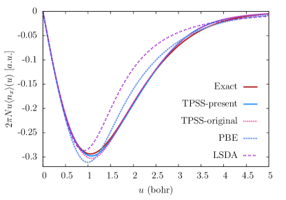
Figure 1: System averaged exchange hole for the LSDA, PBE GGA, and TPSS meta-GGA for the two-electron exponential density. TPSS-original represents the original TPSS hole model of Constantin, Perdew, and Tao tpsshole , while TPSS-present represents the present TPSS hole model. The area under the curve is the exchange energy (in hartree): $E_{\rm x}^{\rm LSDA}=-0.5361$, $E_{\rm x}^{\rm PBE}=-0.6117$, $E_{\rm x}^{\rm TPSS}=-0.6250$, and $E_{\rm x}^{\rm ex}=-0.6250$. Both the original and present TPSS holes yield the same exchange energy, due to the same energy constraint.

IV.2 Gradient dependence of $H(s,z)$

In so-orbital regions where $z\approx 1$ (e.g., core and density tail regions), we assume that the function $H(s,z=1)$ takes the form of

$$H(s,z=1)=\frac{h_{0}+h_{1}s^{2}+h_{2}s^{4}+h_{3}s^{6}}{d_{0}+d_{1}s^{2}+d_{2}s^{4}+d_{3}s^{6}}.$$ (33)

In the large-gradient regime, the function $H(s,z=1)$ should recover the PBE $H(s)$ function Henderson08

$$H^{\rm PBE}(s)=\frac{p_{1}s^{2}+p_{2}s^{4}+p_{3}s^{6}}{1+p_{4}s^{2}+p_{5}s^{4}+p_{6}s^{6}}.$$ (34)

For any density between the two regimes, we take the interpolation formula,

$$H(s,z=1) = \frac{1}{2}{\rm erfc}\bigg{(}\frac{s^{2}-s_{0}^{2}}{s_{0}}\bigg{)}\mathscr{H}(s,z=1)$$ (35)

$$+ \bigg{[}1-\frac{1}{2}{\rm erfc}\bigg{(}\frac{s^{2}-s_{0}^{2}}{s_{0}}\bigg{)}\bigg{]}H^{\rm PBE}(s).~{}~{}~{}~{}~{}~{}$$

Finally, we insert Eq. (35) into Eqs. (30)-(32) and perform the fitting procedure by minimizing the following quantity

$$\sum_{i}u_{i}\bigg{(}\big{\langle}\rho_{\rm x}^{\rm TPSS}(u_{i})\big{\rangle}_{\rm sph}-\big{\langle}\rho_{\rm x}^{\rm exact}(u_{i})\big{\rangle}_{\rm sph}\bigg{)}^{2}$$ (36)

where $\langle\rho_{\rm x}(u)\rangle_{\rm sph}$ is the system average of the exchange hole defined by Eq. (8). It can be expressed in terms of the shape function as $\langle\rho_{\rm x}(u)\rangle_{\rm sph}=(1/N)\int d^{3}rn({\bf r})^{2}J(s,z,u_{f})$. For numerical convenience, we replace the integral with discretsized summation. All the parameters for $H(s,z=1)$ and $H(s)$ are listed in Table 1.

Figure 1 shows the system-averaged exchange hole for the two-electron exponential density evaluated with different hole models, compared to the exact one. We can observe from Fig. 1 that the present TPSS hole is slightly closer to the conventional exact hole than the original TPSS hole, but it is much closer than the PBE GGA and LSDA holes.

IV.3 Infinite barrier model and wave vector analysis for surface energy

For iso-orbital regions, the $s$-dependence of $H(s,z)$ is determined by fitting the model hole to the conventional exact exchange hole for the two-electron exponential density. In the uniform-gas limit, our exchange hole should correctly reduce to the LDA. This requires that $H(s,z)$ vanishes in this limit. To fulfill these considerations, we assume that

$$H(s,z)=H(s,z=1)z^{m},$$ (37)

where $m$ is an integer. In order to determine $m$, we follow the procedure of Ref. tpsshole to study the wave-vector analysis (WVA) of the surface energy. But instead of using the jellium surface model with linearly increasing barrier, here we employ the exactly solvable infinite barrier model (IBM). Since the single-particle density matrix and hence the electron density of IBM is analytically known, this allows us to obtain insight into the $z$-dependence of $H(s,z)$ from this model more easily.

Let us consider a uniform gas of noninteracting electrons subject to the infinite potential barrier perpendicular to the $x$ axis ($V\to\infty$ for $x<0$). The one-particle density matrix is given by LMiglio81 ; IDMoore76

$$\gamma_{1}({\bf r},{\bf r}^{\prime}) = \bar{n}\bigg{[}J(u_{f})-J\bigg{(}\sqrt{u_{f}^{2}+4x_{f}x_{f}^{\prime}}\bigg{)}\bigg{]}\Theta(x)$$ (38)

$$\times \Theta(x^{\prime})$$

where $\Theta(x)$ is a step function, with $\Theta(x)=1$ for $x>0$ and $\Theta(x)=0$ for $x\leq 0$. $\bar{n}$ is the average bulk valence electron density, $x_{f}=xk_{f}$, $x_{f}^{{}^{\prime}}=x^{\prime}k_{f}$, $u_{f}=|{\bf r}-{\bf r}^{\prime}|k_{f}$, and

$$J(\xi)=3j_{1}(\xi)/\xi,$$ (39)

with $j_{1}(\xi)={\rm sin}(\xi)/\xi^{2}-{\rm cos}(\xi)/\xi$ being the first-order spherical Bessel function. The electron density can be obtained from the single-particle density matrix by taking $u=|{\bf r}^{\prime}-{\bf r}|=0$ in Eq. (38). This yields

$$n(x)=\bar{n}[1-J(2x_{f})]\Theta(x).$$ (40)

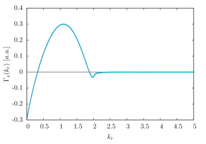
Figure 2: $\Gamma(k)$ of Eq. (44) and smooth fit.

The WVA for the surface exchange energy density is given by tpsshole

$$\gamma_{x}(k)=\int_{0}^{\infty}du~{}8k_{f}u^{2}b_{x}(u)\frac{sin(ku)}{ku}$$ (41)

where

$$b_{x}(u)=\int_{-\infty}^{\infty}dx~{}n(x)\bigg{[}\rho_{x}(x,u)-\rho_{x}^{\rm unif}(u)\bigg{]}.$$ (42)

The exchange hole $\rho_{x}(x,u)$ of IBM can be obtained from the one-particle density matrix of Eq. (38). With some algebra, we can express the WVA surface exchange energy as Langreth82

$$\sigma_{x}=\frac{1}{2}\int_{0}^{\infty}dk_{r}\,\gamma_{x}(k_{r}),$$ (43)

where $k_{r}=k/k_{F}$, and $\gamma_{x}(k_{r})$ is given by

$$\gamma_{x}(k_{r}) = \frac{8}{k_{f}^{2}}\int_{0}^{\infty}du_{f}\,b(u_{f})u_{f}^{2}sinc(k_{r}u_{f})$$ (44)

$$= \frac{1}{(\pi r_{s})^{3}}\Gamma(k_{r}),$$

and

$$b_{x}(u_{f})=-\frac{\bar{n}^{2}}{2k_{f}}\int_{0}^{\infty}dx_{f}\,i_{x}(x_{f},u_{f}).$$ (45)

Here $i_{x}(x_{f},u_{f})=\sum_{l=1}^{6}\chi_{l}(x_{f},u_{f})$, with $\chi_{l}(x_{f},u_{f})$ being defined by Eq. (3.18) of Ref. Langreth82 .

Figure LABEL:Gamma shows $\Gamma(k_{r})$ of Eq. (44). The area under the curve is proportional to the surface exchange energy. From the electron density and density matrix of IBM given by Eqs. (38) and (40), the exact surface exchange energy can be calculated with the WVA of Eq. (43). Langreth and Perdew Langreth82 reported that the value of $\sigma_{x}10^{3}r_{s}^{3}$ is $4.0$ a.u., where $r_{s}$ is Seitz radius. This value is slightly smaller than the value obtained earlier by Harris and Jones Harris74 and Ma and Sahni CQMa79 ($4.1$ a.u.). Our present work gives $3.99$ a.u., which might be the most accurate one.

IV.4 $z$-dependence of $H(s,z)$

The $z$-dependence of $H(s,z)$ [Eq. (37)] can be determined by fitting the TPSS hole to the wave vector analysis. We start with the specific expressions for the local ingredients of the hole model in IBM.

From the electron density of Eq. (40), the reduced density gradient can be explicitly expressed as

$$s(x_{f})=\frac{3}{2x_{f}}\frac{|sinc(2x_{f})-J(2x_{f})|}{[1-J(2x_{f})]^{4/3}}.$$ (46)

The kinetic energy density can be obtained from the single-particle density matrix of Eq. (38). This yields

$$\tau(x_{f}) = k_{f}^{2}\bar{n}\bigg{\{}\frac{3}{10}+\frac{1}{2}J(2x_{f})+\frac{9}{4x_{f}^{2}}[sinc(2x_{f})$$ (47)

$$- J(2x_{f})]\bigg{\}}.$$

Finally, the von Weizäscker kinetic energy density can be expressed as

$$\tau_{W}=\frac{9k_{f}^{2}\bar{n}}{8x_{f}^{2}}\Bigg{\{}\frac{[sinc(2x_{f})-J(2x_{f})]^{2}}{1-J(2x_{f})}\Bigg{\}}.$$ (48)

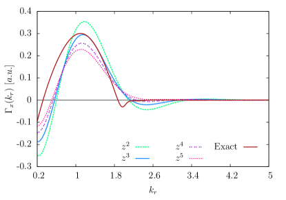
Figure 3: Analysis of $z$-dependence of the WVA for the present TPSS hole of Eq. (29). $z^{3}$ curve provides the best fit to the exact one.

Next, we calculate $\gamma_{x}$ from the TPSS hole. Starting with $b_{x}(u)$ of Eq.(42), we obtain

$$b_{x}(u) = \int_{0}^{\infty}dx\,n(x)\Big{[}\rho_{\rm x}^{\rm TPSS}(x,u)-\rho_{\rm x}^{unif}(u)\Big{]}$$ (49)

$$= \frac{\tilde{n}^{2}}{k_{f}}\int_{0}^{\infty}dx_{f}~{}[1-J(2x_{f})]\bigg{\{}[1-J(2x_{f})]$$

$$\times J^{\rm TPSS}\big{(}u_{f}\sqrt[3]{1-J(2x_{f})},s(x_{f}),z(x_{f})\big{)}$$

$$- J^{\rm unif}(u_{f})\bigg{\}}$$

(Note that $\Theta(x)$ is implicit on the electron density.) Substituting Eq. (49) into Eq. (41), we obtain

$$\gamma_{x}(k)=\frac{8\bar{n}}{3\pi^{2}}\int_{0}^{\infty}dx_{f}~{}\int_{0}^{\infty}du_{f}j_{x}(u_{f},x_{f},k_{r}),$$ (50)

where

$$j_{x} = \varrho(x_{f})\Big{[}\varrho(x_{f})J^{\rm TPSS}\big{(}u_{f}\sqrt[3]{\varrho(x_{f})},s(x_{f}),z(x_{f})\big{)}$$ (51)

$$- J^{\rm unif}(u_{f})\Big{]}sinc(k_{r}u_{f})u_{f}^{2}$$

and $\varrho(x_{f})=1-J(2x_{f})$. Rearrangement of Eq. (50) leads to the final expression

$$\gamma_{x}(k)=\frac{1}{(\pi r_{s})^{3}}\Gamma^{TPSS}(k_{r}),$$ (52)

where

$$\Gamma^{TPSS}(k_{r})=2\int_{0}^{\infty}dx_{f}\,J_{x}(x_{f},k_{r}),$$ (53)

$$J_{x}(x_{f},k_{r})=\int_{0}^{\infty}du_{f}~{}j_{x}(u_{f},x_{f},k_{r}).$$ (54)

Figure 3 shows the comparison of $H(s,z)$ with different choices of $m$ to the exact one. From Fig. 3, we see that the best choice is $m=3$. Figure 4 shows that, compared to the LDA, PBE, and original TPSS holes, the WVA of the present model is in best agreement with the exact one. To further understand these two models, we plot the TPSS shape function of the present and the original models in IBM at $z=0.55$, as shown by Figs. (5) and (6), respectively. From Figs. (5) and (6), we observe that while the present model hole is always negative, the original TPSS hole can be positive at some values of $u_{f}$ and $s$.

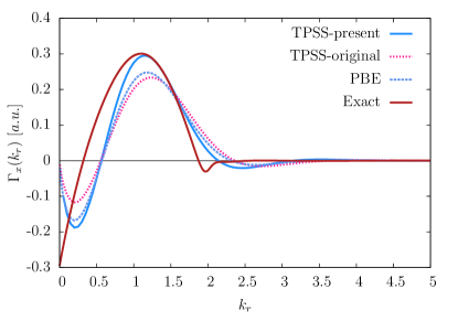
Figure 4: Comparison of the WVA for the present and original TPSS hole models as well as the PBE hole with the exact one. “TPSS-present” represents the present TPSS hole model, while “TPSS-original“ represents the original TPSS model.

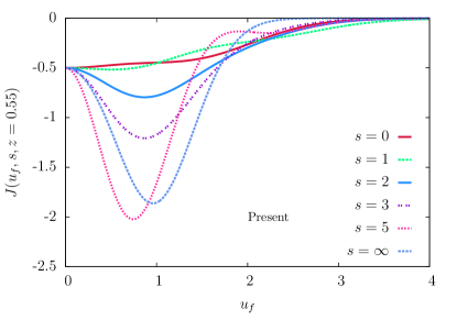
Figure 5: Present TPSS shape function of Eq. (29) for $z=0.55$

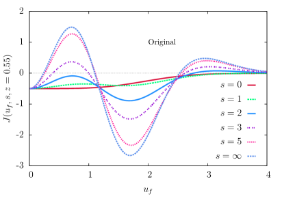
Figure 6: Original TPSS shape function for $z=0.55$

To check our wave vector analysis for the surface exchange energy, we have computed $\sigma_{x}$ from

$$\sigma_{x} = \int_{-\infty}^{\infty}dx\,n(x)\Bigg{[}\epsilon_{x}(n)-\epsilon_{x}^{\rm unif}(\bar{n})\Bigg{]}.$$ (55)

The results are shown in Table 2. From Table 2, we can see that the surface energy from the WVA of the PBE exchange hole shows some inconsistency with the surface energy evaluated directly from the PBE exchange functional with Eq. (55), but the surface energy from the WVA of the TPSS hole (both original and the present version) agrees very well with the surface energy calculated from TPSS exchange functional with Eq. (55). Furthermore, TPSS surface energy is more closer to the exact value than those of the LDA and PBE. The LDA significantly overestimates the surface exchange energy. All these observations are consistent with those evaluated from jellium surface model. It is interesting to note that even the original TPSS shape function in certain range is positive, the surface energy from the original TPSS hole is the same as that from the present model. This result is simply due to the cancellation of the original hole model between positive values and too-negative values at certain $u_{f}$ values, as seen from the comparison of Fig. (6) to (5). The IBM surface energy presents a great challenge to semilocal DFT. It is more difficult to get it right than the surface energy of jellium model with finite linear potential, because the electron density at the surface of IBM is highly inhomogeneous, due to immediate cutoff at surface, and is too far from the slowly varying regime, in which semilocal DFT can be exact (e.g., TPSS functional).

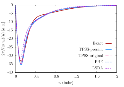
Figure 7: Comparison of various system-averaged hole models for the Ne atom. “TPSS-present” represents the present TPSS hole model, while “TPSS-original” represents the original TPSS model.

Table 2: Comparison of the surface exchange energies (in a.u.) of IBM surface (expressed as $\sigma_{x}{r_{s}}^{3}{10}^{3}$) calculated directly with exchange energy functionals and with the WVA formula. Exact value (obtained in this work) is 3.99 a.u.

	Eq .(55)	WVA integration
LDA	6.318	-
PBE	2.576	2.67
TPSS	2.945	2.95 (original hole)
		2.95 (present hole)

Figure 7 shows the comparison of the LSDA, PBE, and the original and present TPSS exchange hole models to the conventional exact exchange hole of the Ne atom, in which $z$ is in general different from 0 (slowly varying density) and 1 (iso-orbital density). The PBE and LSDA curves are plotted with the hole models of Ref. Henderson08 . From Fig. 7 we can see that the present TPSS hole model is generally closer to the exact one than the original TPSS hole model, while the original TPSS hole model is very close to PBE, but both of them are closer to the exact one than the LSDA.

V TPSS hole in the gauge of the conventional exact exchange

The shape function explicitly depends on the enhancement factor via the energy constraint of Eq. (18). The latter may be altered by arbitrarily adding any amount of the Laplacian of the density without changing the exchange energy. This ambiguity of the exchange energy density KBurke98 leads to the ambiguity of the semilocal exchange hole. Our primary goal of this work is to develop a semilocal exchange hole in the gauge of the conventional exact exchange. This is partly motivated by the fact that in the development of range-separationals, the exact exchange part is usually provided in the conventional gauge.

The exact exchange energy density in the conventional gauge can be conveniently evaluated with the Della Sala-Görling (DSG) DSG01 identity resolution

$$e^{x}_{conv}({\bf r})=\frac{1}{2}\sum_{\mu\nu}Q_{\mu\nu}^{\sigma}\chi_{\mu}({\bf r})\chi_{\nu}^{*}({\bf r}),$$ (56)

where $Q^{\sigma}$ is spin block of DSG matrix tsspg08 . However, many semilocal exchange energy densities or enhancement factors of Eq. (18) are not in the gauge of the conventional exact exchange, due to the constraints such as the Lieb-Oxford bound and the slowly-varying gradient expansion imposed on the enhancement factor. For example, for the two-electron exponential density, the conventionally defined exact enhancement factor is less than 1 near the nucleus, while the TPSS enhancement factor is $F_{\rm x}^{\rm TPSS}\geq 1$ by design. To construct the TPSS exchange hole in the conventional gauge, we can replace the original energy density constraint [Eq. (18)], as used in the construction of the original TPSS exchange hole tpsshole , with the TPSS exchange energy density or enhancement factor in the conventional gauge. In this gauge, the TPSS exchange energy density can be written as tsspg08

$$e_{\rm x}^{\rm TPSS,conv}({\bf r})=e_{\rm x}^{\rm TPSS}({\bf r})-G({\bf r}),$$ (57)

where $e_{x}({\bf r})=n({\bf r})\epsilon_{x}({\bf r})$. Based on the uniform and non-uniform coordinate scaling properties of the exact exchange energy density, Tao, Staroverov, Scuseria, and Perdew (TSSP) tsspg08 proposed a gauge function

$$G({\bf r}) = a\nabla\cdot[f({\bf r})\nabla g({\bf r})],$$ (58)

$$g = \nabla\tilde{\epsilon}$$ (59)

$$f = \frac{n/\tilde{\epsilon}^{2}}{1+c(n/\tilde{\epsilon}^{3})^{2}}\bigg{(}\frac{\tau^{W}}{\tau}\bigg{)}^{b}.$$ (60)

Here $a=0.015$ and $c=0.04$ are determined by a fit to the conventional exact exchange energy density for the H atom, and $b$ is an integer which is chosen to be 4. $\tilde{\epsilon}=-\epsilon_{x}^{\rm ex,conv}$ is the exact exchange energy density in the conventional gauge. This gauge function is integrated to zero, i.e., $\int d^{3}r~{}G({\bf r})=0$, as required. It satisfies the correct uniform coordinate scaling relation, $G_{\lambda}({\bf r})=\lambda^{4}G(\lambda{\bf r})$, and non-uniform scaling relation $G_{\lambda}^{x}(x,y,z)=\lambda G(\lambda x,y,z)$.

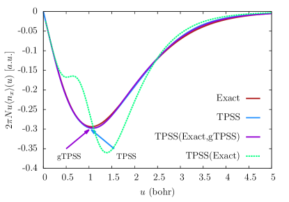
Figure 8: Comparison of the system-average holes for the two-electron exponential density. “Exact” represents the conventional exact system-averaged hole, “TPSS” represents the present TPSS system-averaged hole, “Exact-gTPSS” represents the system-averaged hole generated from the present gauge-corrected TPSS hole model with the conventional exact exchange energy density, and “Exact-TPSS” represents the exact system-averaged hole but it is calculated from the gauge-uncorrected TPSS hole model with the conventional exact exchange energy density.

However, in the density tail ($r\to\infty$) limit of an atom, the exact exchange energy density in the conventional gauge decays as $e_{\rm x}^{\rm ex,conv}\sim-n/2r$, but the TSSP gauge function decays as $G({\bf r})\sim n$. As a result, the exchange energy density in this gauge becomes positive. In order to fix this deficiency, we impose a constraint on the density tail,

$$\lim_{r\to\infty}\frac{G}{e_{\rm x}^{\rm conv}}=0.$$ (61)

This can be achieved by requiring that in the $r\to\infty$ limit, $G$ decays as $n^{p}$ with $p>1$. Here we choose $p=\frac{3}{2}$ and take the same form of the TSSP gauge function, but with $g$ abd $f$ given by

$$g = \nabla\tilde{\epsilon},$$ (62)

$$f = \frac{\Big{(}n/\tilde{\epsilon}^{\frac{7}{3}}\Big{)}^{3/2}}{1+c\Big{(}n/{\tilde{\epsilon}^{3}}\Big{)}^{5/2}}\bigg{(}\frac{\tau^{W}}{\tau}\bigg{)}^{b}.$$ (63)

Here $a=0.01799$ and $c=0.00494$ are determined by fitting the system-averaged hole generated from the present TPSS shape function with the exact enhancement factor in the conventional gauge to the exact system-averaged hole of the two-electron exponential density. The fitting procedure is the same as that in the determination of the $H(s,z=1)$ function. The parameter $b=4$ remains the same as that in the original version of Eq. (60).

Figure 8 shows the comparison of the present TPSS system-averaged exchange hole and the system-averaged exchange hole calculated from the present TPSS hole model with the conventional exact exchange energy density with and without gauge correction of Eqs. (62) and (63 to the exact one. From Fig. 8 we can observe that the exact system-averaged exchange hole generated from the present TPSS hole model simply by replacing the TPSS enhancement factor with the conventional exact exchange enhancement factor without gauge correction significantly deviates from the exact system-averaged hole. However, the agreement can be significantly improved with our gauge correction of Eqs. (62) and (63.

Figure 9 shows the comparison of the TPSS exchange energy density evaluated with the TPSS functional without and with gauge correction to the exact conventional exchange energy density for the two-electron exponential density. From Fig. 9, we can observe that gauge correction is important, leading to a better agreement of the gauge-corrected TPSS exchange energy density with the exact one.

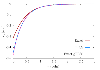
Figure 9: Comparison of the exchange energy densities for the two-electron exponential density calculated with different approximations to the exact one. “TPSS” represents the TPSS exchange energy density calculated directly from the TPSS exchange energy functional. “gTPSS“ represents the gauge-corrected TPSS exchange energy density.

VI Appication to range-separation density functional

As a simple application, we apply the present TPSS hole model to construct a range-separation functional. In general, there are two ways to construct range-separation functionals, depending on the need. For example, we may employ a semilocal DFT for the long-range part, while the exact exchange is used for the short-range part, as pioneered by Heyd, Scuseria and Ernzerhof HSE03 . This kind of range-separation functional is developed for solids, particularly useful for metallic solids, because usual hybrids requires much larger momentum cutoff for metallic systems with electrons nonlocalized. We may employ a semilocal DFT for the short-range part, while the exact exchange is used for the long-range part, as developed by Henderson et al. Henderson08 on the basis of the PBE hole. This kind of range-separation functionals are usually developed for molecular calculations, because the improved long-range part of the exchange hole greatly benefits the description of molecular properties, without significant increase of computational cost. Many range-separation functionals have been proposed hse06 ; Henderson07 ; AVKrukau08 ; Henderson09 ; GalliPRB14 ; Truhlar11 . In the following, we will explore the TPSS hole-based range separation functional with TPSS exchange functional being the long-range (LR) part and the exact exchange being the short-range (SR) part, aiming to improve the TPSS description of two-small band gaps and reaction barrier heights.

The idea of the construction of our TPSS-based range-separation functional is rooted in the constrcution of usual one-parameter hybrid functionals, which, in general, can be written as

$$E_{xc}^{\rm hybrid}=aE_{\rm x}^{\rm HF}+(1-a)E_{\rm x}^{\rm sl}+E_{\rm c}^{\rm sl},$$ (64)

where $a$ is the mixing parameter that controls the amount of exact exchange mixed into a semilocal (sl) functional.

Table 3: Band gaps (in eV) calculated with LSDA, PBE, TPSS, HSE and TPSS-based range-separation functional with $a=0.25$ and $\omega=0.10$ (PW = present work), compared to experiments.

	LSDA	PBE	TPSS	HSE	PW	Exp
C	4.17	4.2	4.24	5.43	5.48	5.48
CdSe	0.31	0.63	0.85	1.48	1.82	1.90
GaAs	0.04	0.36	0.6	1.11	1.44	1.52
GaN	2.15	2.22	2.18	3.48	3.5	3.50
GaP	1.56	1.74	1.83	2.39	2.53	2.35
Ge	-	0.13	0.32	0.8	0.99	0.74
InAs	0	-	0.08	0.57	0.85	0.41
InN	0	0	0	0.72	0.75	0.69
InSb	-	0	-	0.47	0.73	0.23
Si	0.53	0.62	0.71	1.2	1.31	1.17
ZnS	2.02	2.3	2.53	3.44	3.78	3.66
ME	$-.89$	$-0.86$	$-0.76$	$-0.12$	0.14
MAE	0.89	0.86	0.76	0.15	0.17

Table 4: AE6 atomization energies (in kcal/mol) calculated with LSDA, PBE, TPSS, HSE and TPSS-based range-separation functional with $a=0.25$ and $\omega=0.10$ (PW = present work), compared to experimental values PCCP04 .

	LSDA	PBE	TPSS	TPSSh	HSE	PW	Expt
SiH4	347.4	313.2	333.7	333.6	314.5	333.6	322.4
SiO	223.9	195.7	186.7	182.0	182.1	175.4	192.1
S2	135.1	114.8	108.7	105.9	106.3	101.9	101.7
C3H4	802.1	721.2	707.5	704.4	705.9	699.9	704.8
C2H2O2	754.9	665.1	636.0	628.0	635.3	616.4	633.4
C4H8	1304	1168	1156	1154	1152	1152	1149
ME	77.4	12.4	4.1	0.75	$-1.2$	$-4.0$
MAE	77.4	15.5	5.9	6.1	4.8	8.8

Following the prescription of Heyd, Scuseria and Ernzerhof (HSE) HSE03 , we write the TPSS-based range-separation functional as

$$E_{\rm xc}=aE_{\rm x}^{\rm HF,SR}+(1-a)E_{\rm x}^{\rm sl,SR}+E_{\rm x}^{\rm sl,LR}+E_{\rm c}^{\rm sl},$$ (65)

where $E_{\rm x}^{\rm HF,SR}$ is the Hartree-Fock (HF) exchange serving as part of the short-range contribution, while $E_{\rm x}^{\rm sl,SR}$ is the TPSS exchange that provides the rest of the short-range contribution. $E_{\rm c}^{\rm sl}$ is TPSS correlation. The long-range contribution is provided fully by the TPSS exchange $E_{\rm x}^{\rm sl,LR}$. They are given, respectively, by

$$\epsilon_{\rm X}^{{\rm HF,SR}}=\frac{1}{2}\int_{0}^{\infty}du~{}4\pi u^{2}h_{\rm X}^{\rm HF}({\bf r},u)\frac{{\rm erfc}(\omega u)}{u},$$ (66)

$$\epsilon_{\rm X}^{{\rm sl,SR}}=\frac{1}{2}\int_{0}^{\infty}du~{}4\pi u^{2}h_{\rm X}^{\rm DFT}({\bf r},u)\frac{{\rm erfc}(\omega u)}{u},$$ (67)

$$\epsilon_{\rm X}^{{\rm sl,LR}}=\frac{1}{2}\int_{0}^{\infty}du~{}4\pi u^{2}h_{\rm X}^{\rm DFT}({\bf r},u)\frac{{\rm erf}(\omega u)}{u},$$ (68)

where $\omega$ is a range-separation parameter, and ${\rm erf}(x)$ is the error function defined by Eq. (28). From Eqs. (65)-(68), we can see that the amount of exact exchange mixing is controlled by two parameters $a$ and $\omega$. Determination of them is discussed below. To test this functional, we have implemented it into the development version of Gaussian 09 gaussian09 .

Table 5: BH6 reaction barrier heights (in kcal/mol) calculated with PBE, TPSS, HSE and TPSS-based range-separation functional with $a=0.25$ and $\omega=0.10$ (PW = present work), in comparison with reference values JPaier10 ; JPCA03 . f(r) = forward (reverse) barrier height.

	PBE	TPSS	TPSSh	HSE	PW	Ref
OH + CH4 $\rightarrow$ CH3 + H2O	$-5.29$	$-0.97$	1.50	1.96	4.86	6.54(f)
	8.95	9.90	11.79	13.9	14.3	19.6(r)
H + OH $\rightarrow$ O + H2	3.69	$-1.56$	$-0.15$	7.06	1.75	10.5(f)
	$-1.47$	4.73	6.90	5.93	9.89	12.9(r)
H + H2S $\rightarrow$ H2 + HS	$-1.20$	$-4.55$	$-3.72$	1.03	$-2.64$	3.55(f)
	9.40	12.72	13.4	12.4	14.4	17.3(r)
ME	$-9.37$	$-8.34$	$-6.76$	$-4.66$	$-4.63$
MAE	9.37	8.34	6.76	4.66	4.63

In the TPSS-based hybrid functional TPSSh, $a=0.1$ was fitted to molecular properties. In other words, in TPSSH, the optimized of $a$ is 0.1. So, in the TPSS-based range-separation functional of Eq. (65), the best value of $\omega$ will be 0, if $a=0.1$ is chosen. Since in the range-separation functional, some amount of the exact exchange (here the long-range part) in TPSSh is replaced by semilocal TPSS functional, to compensate for this, we need a value of $a$ larger than 0.1. Then we can find the best range-separation parameter $\omega$ by fitting to some electronic properties. To avoid possible overfitting, here we choose $a=1/4$, a value that was recommended by Perdew, Ernzerhof, and Burke Perdew96 and adopted with PBE0 functional PBE0 . The parameter $\omega$ is determined by a fit to the band gap of diamond (C). This yields $\omega=0.1$. Then we apply this range-separation functional to calculate the band gaps of 10 semiconductors. The results are listed in Table 3. From Table 3, we see that the band gaps of this range-separation functional is remarkably accurate, with a mean absolute deviation from experiments of only $0.17$ eV, about the same accuracy of HSE functional. We can also see from Table 3 that this TPSS-based range-separation functional should provide more accurate description for large band-gap materials, and therefore it provides an alternative choice for band-gap and other solid-state calculations.

Next, we apply our range-separation functional to calculate atomization energies of AE6 molecules. The results are listed in Tables 4. From Tables 4, we can see that, our range-separation functional only worsens the TPSS atomization energies of TPSS functional for this special set by about 3 kcal/mol. This error is still smaller than many other DFT methods such as LSDA, PBE, and PBEsol.

Reaction barrier heights are decisive quantity in the study of chemical kinetics. However, semilocal functionals tend to underestimate this quantity. As an interesting application, we apply our range-separation functional to calculate representative reaction barrier heights of BH6, which consists of three forward (f) and three reverse (r) barrier heights. The results are listed in Table 5. For comparison, we also calculated these barrier heights using PBE, TPSS, TPSSh, and HSE. From Table 5, we obserce that our range-separation functional provides the most accurate description of BH6, compared to other functionals considered.

VII Conclusion

In conclusion, we have developed a semilocal exchange hole underlying TPSS exchange functional. The hole is exact in the uniform-gas limit and accurate for iso-orital densities. Then is is interpolated between these two densities through WVA on the surface of infinite barrier model. Our numerical test on the Ne atom shows that the hole mimics the conventional exact exchange hole quite accurately. In particular, with our new gauge function correction, the hole model can generate the system-averaged hole from the conventional exact exchange energy density in good agreement with the present TPSS hole and the exact hole for the two-electron exponential density.

Based on the TPSS hole, we have constructed a range-separation functional. This functional yields very accurate band gaps and reaction barrier heights, without losing much accuracy on atomization energies. This accuracy makes this functional an attractive alternative in solid-state calculations and molecular kinetics.

References

- (1) W. Kohn and L.J. Sham, Phys. Rev. 140, A1133 (1965).
- (2) R.G. Parr and W. Yang, Density Functional Theory of Atoms and Molecules (Oxford University Press, New York, 1989).
- (3) R.M. Dreizler and E.K.U. Gross, Density Functional Theory (Springer, Berlin, 1990).
- (4) J.P. Perdew and Y. Wang, Phys. Rev. B 33, 8800 (1986).
- (5) A.D. Becke, Phys. Rev. A 38, 3098 (1988).
- (6) C. Lee, W. Yang, and R.G. Parr, Phys. Rev. B 37, 785 (1988).
- (7) A.D. Becke and M. R. Roussel, Phys. Rev. A 39, 3761 (1989).
- (8) A.D. Becke, J. Chem. Phys. 104, 1040 (1996).
- (9) P.J. Stephens, F.J. Devlin, C.F. Chabalowski, and M.J. Frisch, J. Phys. Chem. 98, 11623 (1994).
- (10) J.P. Perdew, K. Burke, and M. Ernzerhof, Phys. Rev. Lett. 77, 3865 (1996).
- (11) T.V. Voorhis and G.E. Scuseria, J. Chem. Phys. 109, 400 (1998).
- (12) F.A. Hamprecht, A.J. Cohen, D.J. Tozer, and N.C. Handy, J. Chem. Phys. 109, 6264 (1998).
- (13) M. Ernzerhof and G.E. Scuseria, J. Chem. Phys. 110, 5029 (1999).
- (14) J. Heyd, G.E. Scuseria, and M. Ernzerhof, J. Chem. Phys. 118, 8207 (2003).
- (15) R. Armiento and A.E. Mattsson, Phys. Rev. B 72, 085108 (2005).
- (16) Y. Zhao and D.G. Truhlar, J. Chem. Phys. 125, 194101 (2006).
- (17) J. Tao, J.P. Perdew, V.N. Staroverov, and G.E. Scuseria, Phys. Rev. Lett. 91, 146401 (2003).
- (18) J.P. Perdew, A. Ruzsinszky, G.I. Csonka, L.A. Constantin, and J. Sun, Phys. Rev. Lett. 103, 026403 (2009).
- (19) J.P. Perdew, A. Ruzsinszky, G.I. Csonka, O.A. Vydrov, G.E. Scuseria, L.A. Constantin, X. Zhou, and K. Burke, Phys. Rev. Lett. 100, 136406 (2008).
- (20) J. Sun, A. Ruzsinszky, and J.P. Perdew, Phys. Rev. Lett. 115, 036402 (2015).
- (21) A.V. Arbuznikov and M. Kaupp, J. Chem. Phys. 141, 204101 (2014).
- (22) J. Tao and Y. Mo, Phys. Rev. Lett. 117, 073001 (2016).
- (23) S.H. Vosko, L. Wilk, and M. Nusair, Can. J. Phys. 58, 1200 (1980).
- (24) J.P. Perdew and Y. Wang, Phys. Rev. B 45, 13244 (1992).
- (25) J.P. Perdew, J.A. Chevary, S.H. Vosko, K.A. Jackson, M.R. Pederson, D.J. Singh, and C. Fiolhais, Phys. Rev. B 46, 6671 (1992).
- (26) Z. Wu and R.E. Cohen, Phys. Rev. B 73, 235116 (2006).
- (27) C.J. Cramer and D.G. Truhlar, Phys.Chem.Chem.Phys. 11, 10757 (2009).
- (28) R. Peverati and D.G. Truhlar, Phys. Phil.Trans. R. Soc. A 372, 20120476 (2011).
- (29) A.J. Cohen, P. Mori-Sanchez, and W. Yang, Chem.Rev. 112, 289 (2012).
- (30) A.D. Becke, J. Chem. Phys. 140, 18A301 (2014).
- (31) V.N. Staroverov, G.E. Scuseria, J. Tao, and J.P. Perdew, J. Chem. Phys. 119, 12129 (2003); 121, 11507(E) (2004).
- (32) P. Hao, J. Sun, B. Xiao, A. Ruzsinszky, G.I. Csonka, J. Tao, S. Glindmeyer, and J.P. Perdew, J. Chem. Theory Comput. 9, 355 (2013).
- (33) L. Goerigk and S. Grimme, J. Chem. Theory Comput. 6, 107 (2010).
- (34) L. Goerigk and S. Grimme, J. Chem. Theory Comput. 7, 291 (2011).
- (35) D. Jacquemin and C. Adamo, J. Chem. Theory Comput. 7, 369 (2011).
- (36) Y. Mo, G. Tian, R. Car, V.N. Staroverov, G.E. Scuseria, and J. Tao, submitted.
- (37) G.I. Csonka, J.P. Perdew, A. Ruzsinszky, P.H.T. Philipsen, S. Lebégue, J. Paier, O.A. Vydrov, and J.G. Ángyán Phys. Rev. B 79, 155107 (2009).
- (38) P. Haas, F. Tran, and P. Blaha, Phys. Rev. B 79, 085104 (2009).
- (39) F. Tran, J. Stelzl, and P. Blaha, J. Chem. Phys. 144, 204120 (2016).
- (40) V.N. Staroverov, G.E. Scuseria, J. Tao, and J.P. Perdew, Phys. Rev. B 69, 075102 (2004).
- (41) J.P. Perdew, V.N. Staroverov, J. Tao, and G.E. Scuseria, Phys. Rev. A 78, 052513 (2008).
- (42) J. Jaramillo, G.E. Scuseria, and M. Ernzerhof, J. Chem. Phys. 118, 1068 (2003).
- (43) R. Peverati and D.G. Truhlar, Phys. Chem. Lett. 2, 2810 (2011).
- (44) Phys. Rev. B 54, 16533 (1996).
- (45) J. Tao, Density Functional Theory of Atoms, Molecules, and Solids (VDM Verlag, Germany, 2010).
- (46) M. Ernzerhof and J.P. Perdew J. Chem. Phys. 109, 3313 (1998).
- (47) L.A. Constantin, J.P. Perdew, and J. Tao, Phys. Rev. B 73, 205104 (2006).
- (48) L.A. Constantin, E. Fabiano, and F. Della Sala Phys. Rev. B 88, 125112 (2013).
- (49) Phys. Rev. B 84, 075144 (2011).
- (50) Ann. Rev. Phys. Chem. 61, 85 (2010).
- (51) M. Modrzejewski, M. Hapka, G. Chalasinski, and M.M. Szczesniak, J. Chem. Theory Comput., 12, 3662 (2016).
- (52) L. Schimka, J. Harl, and G. Kresse, J. Chem. Phys. 134, 024116 (2011).
- (53) J. Tao, J.P. Perdew, V.N. Staroverov, and G.E. Scuseria, Phys. Rev. A 77, 012509 (2008).
- (54) G.L. Oliver and J.P. Perdew, Phys. Rev. A 20, 397 (1979).
- (55) K. Burke, F.G. Cruz, and K.-C. Lam, J. Chem. Phys. 109, 8161 (1998).
- (56) J.P. Perdew, S. Kurth, A. Zupan, and P. Blaha, Phys. Rev. Lett. 82, 2544 (1999).
- (57) J. Tao, S. Liu, Z. Fan, and A.M. Rappe, Phys. Rev. B 92, 060401(R) (2015).
- (58) T.M. Henderson, B.G. Janesko, and G.E. Scuseria, J. Chem. Phys. 128, 194105 (2008).
- (59) L. Miglio, M.P. Tosi, and N.H. March, Sur. Sci. 111, 119 (1981).
- (60) I.D. Moore and N.H. March, Ann. Phys. 97, 136 (1976).
- (61) D.C. Langreth and J.P. Perdew, Phys. Rev. B 26, 2810 (1982).
- (62) J. Harris and R.O. Jones, J. Phys. F 4, 1170 (1974).
- (63) C.Q. Ma and V. Sahni, Phys. Rev. B 20, 2291 (1979).
- (64) F. Della Sala and A. Görling, J. Chem. Phys. 115, 5718 (2001).
- (65) A.V. Krukau, O.A. Vydrov, A.F. Izmaylov, and G.E. Scuseria, J. Chem. Phys. 125, 224106 (2006).
- (66) T.M. Henderson, A.F. Izmaylov, G.E. Scuseria, and A. Savin, J. Chem. Phys. 127, 221103 (2007).
- (67) A.V. Krukau, G.E. Scuseria, J.P. Perdew, and A. Savin, J. Chem. Phys. 129, 124103 (2008).
- (68) T.M. Henderson, B.G. Janesko, G.E. Scuseria, and A. Savin, Int. J. Quantum Chem. 109, 2023 (2009).
- (69) J.H. Skone, M. Govoni, and G. Galli, Phys. Rev. B 89, 195112 (2014).
- (70) Y. Zhao, J. Pu, B.J. Lynch, and D.G. Truhlar, Phys. Chem. Chem. Phys. 6, 673 (2004).
- (71) J. Paier, B.G. Janesko, T.M. Henderson, G.E. Scuseria, A. Güneis, and G. Kresse, J. Chem. Phys. 132, 094103 (2010).
- (72) B.J. Lynch and D.G. Truhlar, J. Phys. Chem. A 107, 8996 (2003).
- (73) Gaussian Development Version, Revision B.01, M.J. Frisch et al., Gaussian, Inc., Wallingford CT (2009).
- (74) J.P. Perdew, M. Ernzerhof, and K. Burke, J. Chem. Phys. 105, 9982 (1996).