Matrix Product State for Higher-Order Tensor Compression and Classification

Abstract

This paper introduces matrix product state (MPS) decomposition as a new and systematic method to compress multidimensional data represented by higher-order tensors. It solves two major bottlenecks in tensor compression: computation and compression quality. Regardless of tensor order, MPS compresses tensors to matrices of moderate dimension which can be used for classification. Mainly based on a successive sequence of singular value decompositions (SVD), MPS is quite simple to implement and arrives at the global optimal matrix, bypassing local alternating optimization, which is not only computationally expensive but cannot yield the global solution. Benchmark results show that MPS can achieve better classification performance with favorable computation cost compared to other tensor compression methods.

I Introduction

There is an increasing need to handle large multidimensional datasets that cannot efficiently be analyzed or processed using modern day computers. Due to the curse of dimensionality it is urgent to develop mathematical tools which can evaluate information beyond the properties of large matrices [1]. The essential goal is to reduce the dimensionality of multidimensional data, represented by tensors, with a minimal information loss by compressing the original tensor space to a lower-dimensional tensor space, also called the feature space [1]. Tensor decomposition is the most natural tool to enable such compressions [2].

Until recently, tensor compression is merely based on Tucker decomposition (TD) [3], also known as higher-order singular value decomposition (HOSVD) when orthogonality constraints on factor matrices are imposed [4]. TD is also an important tool for solving problems related to feature extraction, feature selection and classification of large-scale multidimensional datasets in various research fields. Its well-known application in computer vision was introduced in [5] to analyze some ensembles of facial images represented by fifth-order tensors. In data mining, the HOSVD was also applied to identify handwritten digits [6]. In addition, the HOSVD has been applied in neuroscience, pattern analysis, image classification and signal processing [7, 8, 9]. The higher-order orthogonal iteration (HOOI) [10] is an alternating least squares (ALS) for finding the TD approximation of a tensor. Its application to independent component analysis (ICA) and simultaneous matrix diagonalization was investigated in [11]. Another TD-based method is multilinear principal component analysis (MPCA) [12], an extension of classical principal component analysis (PCA), which is closely related to HOOI. Meanwhile, TD suffers the following conceptual bottlenecks in tensor compression:

• Computation. TD compresses an $N$th-order tensor in tensor space $\mathbb{R}^{I_{1}\times I_{2}\times\cdots I_{N}}$ of large dimension $I=\prod_{j=1}^{N}I_{j}$ to its $N$th-order core tensor in a tensor space $\mathbb{R}^{\Delta_{1}\times\Delta_{2}\times\cdots\Delta_{N}}$ of smaller dimension $N_{f}=\prod_{j=1}^{N}\Delta_{j}$ by using $N$ factor matrices of size $I_{j}\times\Delta_{j}$. Computation of these $N$ factor matrices is computationally intractable. Instead, each factor matrix is alternatingly optimized with all other $N-1$ factor matrices held fixed, which is still computationally expensive. Practical application of the TD-based compression is normally limited to small-order tensors.

• Compression quality. TD is an effective representation of a tensor only when the dimension of its core tensor is fairly large [2]. Restricting dimension $N_{f}=\prod_{j=1}^{N}\Delta_{j}$ to a moderate size for tensor classification results in significant lossy compression, making TD-based compression a highly heuristic procedure for classification. It is also almost impossible to tune $\Delta_{j}\leq I_{j}$ among $\prod_{j=1}^{N}\Delta_{j}\leq\bar{N}_{f}$ for a prescribed $\bar{N}_{f}$ to have a better compression.

In this paper, we introduce the matrix product state (MPS) decomposition [13, 14, 15, 16] as a new method to compress tensors, which fundamentally circumvent all the above bottlenecks of TD-based compression. Namely,

• Computation. The MPS decomposition is fundamentally different from the TD in terms of its geometric structure as it is made up of local component tensors with maximum order three. Consequently, using the MPS decomposition for large higher-order tensors can potentially avoid the computational bottleneck of the TD and related algorithms. Computation for orthogonal common factors in MPS is based on successive SVDs without any recursive local optimization procedure and is very efficient with low-cost.

• Compression quality. MPS compresses $N$th-order tensors to their core matrices of size $\mathbb{R}^{N_{1}\times N_{2}}$. The dimension $N_{f}=N_{1}N_{2}$ can be easily tuned to a moderate size with minimum information loss by pre-positioning the core matrix in the MPS decomposition.

MPS has been proposed and applied to study quantum many-body systems with great success, prior to its introduction to the mathematics community under the name tensor-train (TT) decomposition [17]. However, to the best of our knowledge its application to machine learning and pattern analysis has not been proposed.

Our main contribution is summarized as follows:

• Propose MPS decomposition as a new and systematic method for compressing tensors of arbitrary order to matrices of moderate dimension, which circumvents all existing bottlenecks in tensor compression;

• Develop MPS decomposition tailored for optimizing the dimensionality of the core matrices and the compression quality. Implementation issues of paramount importance for practical computation are discussed in detail. These include tensor mode permutation, tensor bond dimension control, and positioning the core matrix in MPS;

• Extensive experiments are performed along with comparisons to existing state-of-the-art tensor classification methods to show its advantage.

A preliminary result of this work was presented in [18]. In the present paper, we rigorously introduce the MPS as a new and systematic approach to tensor compression for classification, with computational complexity and efficiency analysis. Furthermore, new datasets as well a new experimental design showcasing computational time and classification success rate (CSR) benchmarks are included.

The rest of the paper is structured as follows. Section II provides a rigorous mathematical analysis comparing MPS and TD in the context of tensor compression. Section III is devoted to MPS tailored for effective tensor compression, which also includes a computational complexity analysis comparing MPS to HOOI, MPCA and uncorrelated multilinear discriminant analysis with regularization (R-UMLDA) [19]. In Section IV, experimental results are shown to benchmark all algorithms in classification performance and training time. Lastly, Section V concludes the paper.

II MPS decomposition vs TD decomposition in tensor compression

We introduce some notations and preliminaries of multilinear algebra [2]. Zero-order tensors are scalars and denoted by lowercase letters, e.g., $x$. A first-order tensor is a vector and denoted by boldface lowercase letters, e.g., x. A matrix is a second-order tensor and denoted by boldface capital letters, e.g., X. A higher-order tensor (tensors of order three and above) are denoted by boldface calligraphic letters, e.g., $\bm{\mathcal{X}}$. Therefore, a general Nth-order tensor of size $I_{1}\times I_{2}\times\cdots\times I_{N}$ can be defined as $\bm{\mathcal{X}}\in\mathbb{R}^{I_{1}\times I_{2}\times\cdots\times I_{N}}$, where each $I_{i}$ is the dimension of its mode $i$. We also denote $x_{i}$, $x_{ij}$ and $x_{i_{1}\cdots i_{N}}$ as the $i$th entry $\textbf{x}(i)$, $(i,j)$th entry $\textbf{X}(i,j)$ and $(i_{1},\cdots,i_{N})$th entry $\bm{\mathcal{X}}(i_{1},\cdots,i_{N})$ of vector x, matrix X and higher-order tensor $\bm{\mathcal{X}}$, respectively.

Mode-$n$ matricization (also known as mode-$n$ unfolding or flattening) of $\bm{\mathcal{X}}$ is the process of unfolding or reshaping $\bm{\mathcal{X}}$ into a matrix $\textbf{X}_{(n)}\in\mathbb{R}^{I_{n}\times(\prod_{i\neq n}I_{i})}$ such that $\textbf{X}_{(n)}(i_{n},j)=\bm{\mathcal{X}}(i_{1},\cdots,i_{n},\cdots,i_{N})$ for $j=1+\sum_{k=1,k\neq n}^{N}(i_{k}-1)\prod_{m=1,m\neq n}^{k-1}I_{m}$. We also define the dimension of $\bm{\mathcal{X}}$ as $\prod_{n=1}^{N}I_{n}$. The mode-$n$ product of $\bm{\mathcal{X}}$ with a matrix $\textbf{A}\in\mathbb{R}^{J_{n}\times I_{n}}$ is denoted as $\bm{\mathcal{X}}\times_{n}\textbf{A}$, which is a $N$th-order tensor of size $I_{1}\times\cdots\times I_{n-1}\times J_{n}\times I_{n+1}\times\cdots\times I_{N}$ such that

$$\begin{array}[]{ll}(\bm{\mathcal{X}}\times_{n}\textbf{A})(i_{1},\cdots,i_{n-1},j_{n},i_{n+1},\cdots,i_{N})&=\\ \displaystyle\sum_{i_{n}=1}^{I_{n}}\bm{\mathcal{X}}(i_{1},\cdots,i_{n},\cdots i_{N})\textbf{A}(j_{n},i_{n}).&\end{array}$$

The Frobenius norm of $\bm{\mathcal{X}}$ is defined as $||\bm{\mathcal{X}}||_{F}=(\sum_{i_{1}=1}^{I_{1}}\sum_{i_{2}=1}^{I_{2}}\cdots\sum_{i_{N}=1}^{I_{N}}x^{2}_{i_{1}i_{2}\cdots i_{N}})^{1/2}$.

We are concerned with the following problem of tensor compression for supervised learning :

Based on $K$ training Nth-order tensors $\bm{\mathcal{X}}^{(k)}\in\mathbb{R}^{I_{1}\times I_{2}\times\cdots\times I_{N}}$ ($k=1,2,\ldots,K$), find common factors to compress both training tensor $\bm{\mathcal{X}}^{(k)}$ and test tensors $\bm{\mathcal{Y}}^{(\ell)}$ ($\ell=1,\cdots,L$) to a feature space of moderate dimension to enable classification.

Until now, only TD has been proposed to address this problem [7]. More specifically, the $K$ training sample tensors are firstly concatenated along the mode $(N+1)$ to form an $(N+1)$th-order tensor $\bm{\mathcal{X}}$ as

$$\bm{\mathcal{X}}=[\bm{\mathcal{X}}^{(1)}\bm{\mathcal{X}}^{(2)}\cdots\bm{\mathcal{X}}^{(K)}]\in\mathbb{R}^{I_{1}\times I_{2}\times\cdots\times I_{N}\times K}.$$ (1)

TD-based compression such as HOOI [10] is then applied to have the approximation

$$\bm{\mathcal{X}} \approx \bm{\mathcal{R}}\times_{1}\textbf{U}^{(1)}\times_{2}\textbf{U}^{(2)}\cdots\times_{N}\textbf{U}^{(N)},$$ (2)

where each matrix $\textbf{U}^{(j)}\in\mathbb{R}^{I_{j}\times\Delta_{j}}$ $(j=1,2,\ldots,N)$ is orthogonal, i.e. $\textbf{U}^{(j)T}\textbf{U}^{(j)}=\textbf{I}$ ($\textbf{I}\in\mathbb{R}^{\Delta_{j}\times\Delta_{j}}$ denotes the identity matrix). It is called a common factor matrix and can be thought of as the principal components in each mode $j$. The parameters $\Delta_{j}$ satisfying

$$\Delta_{j}\leq\text{rank}(\textbf{X}_{(j)})$$ (3)

are referred to as the compression ranks of the TD.
The $(N+1)$th-order core tensor $\bm{\mathcal{R}}$ and common factor matrices $\textbf{U}^{(j)}\in\mathbb{R}^{I_{j}\times\Delta_{j}}$ are supposed to be found from the following nonlinear least squares

$$\begin{array}[]{r}\displaystyle\min_{\begin{subarray}{c}\bm{\mathcal{R}}\in\mathbb{R}^{\Delta_{1}\times\cdots\times\Delta_{N}\times K},\\ \textbf{U}^{(j)}\in\mathbb{R}^{I_{j}\times\Delta_{j}},j=1,...,N\end{subarray}}\Phi(\bm{\mathcal{R}},\textbf{U}^{(1)},\cdots,\textbf{U}^{(N)})\\ \mbox{subject to}\quad(\textbf{U}^{(j)})^{T}\textbf{U}^{(j)}=\textbf{I},j=1,...,N,\end{array}$$ (4)

where $\Phi(\bm{\mathcal{R}},\textbf{U}^{(1)},\cdots,\textbf{U}^{(N)}):=||\bm{\mathcal{X}}-\bm{\mathcal{R}}\times_{1}\textbf{U}^{(1)}\times_{2}\textbf{U}^{(2)}\cdots\times_{N}\textbf{U}^{(N)}||_{F}^{2}$ The optimization problem (4) is computationally intractable, which could be addressed only by alternating least squares (ALS) in each $\textbf{U}^{(j)}$ (with other $\textbf{U}^{(\ell)}$, $\ell\neq j$ held fixed) [10]:

$$\begin{array}[]{r}\displaystyle\min_{\begin{subarray}{c}\bm{\mathcal{R}}^{(j)}\in\mathbb{R}^{\Delta_{1}\times\cdots\times\Delta_{N}\times K},\\ \textbf{U}^{(j)}\in\mathbb{R}^{I_{j}\times\Delta_{j}}\end{subarray}}\Phi^{(j)}(\bm{\mathcal{R}}^{(j)},\textbf{U}^{(j)})\\ \mbox{subject to}\quad(\textbf{U}^{(j)})^{T}\textbf{U}^{(j)}=\textbf{I},\end{array}$$ (5)

where $\Phi^{(j)}(\bm{\mathcal{R}}^{(j)},\textbf{U}^{(j)}):=||\bm{\mathcal{X}}-\bm{\mathcal{R}}^{(j)}\times_{1}\textbf{U}^{(1)}\times_{2}\textbf{U}^{(2)}\cdots\times_{N}\textbf{U}^{(N)}||_{F}^{2}$. The computation complexity per one iteration consisting of $N$ ALS (5) is [20, p. 127]

$$\mathcal{O}(K\Delta I^{N}+NKI\Delta^{2(N-1)}+NK\Delta^{3(N-1)})$$ (6)

for

$$I_{j}\equiv I\quad\mbox{and}\quad\Delta_{j}\equiv\Delta,j=1,2,...,N.$$ (7)

The optimal $(N+1)$th-order core tensor $\bm{\mathcal{R}}\in\mathbb{R}^{\Delta_{1}\times\cdots\times\Delta_{N}\times K}$ in (4) is seen as the concatenation of compressed $\widetilde{\bm{\mathcal{X}}}^{(k)}\in\mathbb{R}^{\Delta_{1}\times\cdots\times\Delta_{N}}$ of the sample tensors $\bm{\mathcal{X}}^{(k)}\in\mathbb{R}^{I_{1}\times\cdots\times I_{N}}$, $k=1,\cdots,K$:

$$\bm{\mathcal{R}}=[\widetilde{\bm{\mathcal{X}}}^{(1)}\widetilde{\bm{\mathcal{X}}}^{(2)}\cdots\widetilde{\bm{\mathcal{X}}}^{(N)}]=\bm{\mathcal{X}}\times_{1}(\textbf{U}^{(1)})^{T}\cdots\times_{N}(\textbf{U}^{(N)})^{T}.$$ (8)

Accordingly, the test tensors $\bm{\mathcal{Y}}^{(\ell)}$ are compressed to

$$\widetilde{\bm{\mathcal{Y}}}^{(\ell)}=\bm{\mathcal{Y}}^{(\ell)}\times_{1}(\textbf{U}^{(1)})^{T}\cdots\times_{N}(\textbf{U}^{(N)})^{T}\in\mathbb{R}^{\Delta_{1}\times\cdots\times\Delta_{N}}.$$ (9)

The number

$$N_{f}=\prod_{j=1}^{N}\Delta_{j}$$ (10)

thus represents the dimension of the feature space $\mathbb{R}^{\Delta_{1}\times\cdots\times\Delta_{N}}$.
Putting aside the computational intractability of the optimal factor matrices $\textbf{U}^{(j)}$ in (4), the TD-based tensor compression by (8) and (9) is a systematic procedure only when the right hand side of (2) provides a good approximation of $\bm{\mathcal{X}}$, which is impossible for small $\Delta_{j}$ satisfying (3) [2]. In other words, the compression of large dimensional tensors to small dimensional tensors results in substantial lossy compression under the TD framework. Furthermore, one can see the value of (5) is lower bounded by

$$\sum_{i=1}^{r_{j}-\Delta_{j}-1}s_{i},$$ (11)

where $r_{j}:=\text{rank}(\bm{\mathcal{X}}_{(j)})$ and $\{s_{r_{j}},\cdots,s_{1}\}$ is the set of non-zero eigenvalues of the positive definite matrix $\bm{\mathcal{X}}_{(j)}(\bm{\mathcal{X}}_{(j)})^{T}$ in decreasing order. Since the matrix $\bm{\mathcal{X}}_{(j)}\in\mathbb{R}^{I_{j}\times(K\prod_{\ell\neq j}I_{\ell})}$ is highly unbalanced as a result of tensor matricization along one mode versus the rest, it is almost full-row (low) rank ($r_{j}\approx I_{j}$) and its squared $\bm{\mathcal{X}}_{(j)}(\bm{\mathcal{X}}_{(j)})^{T}$ of size $I_{j}\times I_{j}$ is well-conditioned in the sense that its eigenvalues do not decay quickly. As a consequence, (11) cannot be small for small $\Delta_{j}$ so the ALS (5) cannot result in a good approximation. The information loss with the least square (5) is thus more than

$$-\sum_{i=1}^{r_{j}-\Delta_{j}-1}\frac{s_{i}}{\sum_{i=1}^{r_{j}}s_{i}}\log_{2}\frac{s_{i}}{\sum_{i=1}^{r_{j}}s_{i}},$$ (12)

which is really essential in the von Neumann entropy [21] of $\bm{\mathcal{X}}_{(j)}$:

$$-\sum_{i=1}^{r_{j}}\frac{s_{i}}{\sum_{i=1}^{r_{j}}s_{i}}\log_{2}\frac{s_{i}}{\sum_{i=1}^{r_{j}}s_{i}}.$$ (13)

Note that each entropy (13) quantifies only local correlation between mode $j$ and the rest [22]. The MPCA [12] aims at (4) with

$$\bm{\mathcal{X}}=[(\bm{\mathcal{X}}^{(1)}-\bar{\bm{\mathcal{X}}})\cdots(\bm{\mathcal{X}}^{(K)}-\bar{\bm{\mathcal{X}}})]$$

with $\bar{\bm{\mathcal{X}}}=\frac{1}{K+L}(\sum_{k=1}^{K}\bm{\mathcal{X}}^{(k)}+\sum_{\ell=1}^{L}\bm{\mathcal{Y}}^{\ell)})$. With such definition of $\bm{\mathcal{X}}$, $(N+1)$th-order core tensor $\bm{\mathcal{X}}$ is the concatenation of principal components of $\bm{\mathcal{X}}^{(k)}$, while principal components of $\bm{\mathcal{Y}}^{(\ell)}$ is defined by $(\bm{\mathcal{Y}}^{(\ell)}-\bar{\bm{\mathcal{X}}})\times_{1}(\bm{U}^{(1)})^{T}\cdots\times_{N}(\bm{U}^{(N)})^{T}$. Thus, MPCA suffers the similar conceptual drawbacks inherent by TD. Particularly, restricting $N_{f}=\prod_{j=1}^{N}\Delta_{j}$ to a moderate size leads to ignoring many important principle components.

We now present a novel approach to extract tensor features, which is based on MPS. Firstly, permute all modes of the tensor $\bm{\mathcal{X}}$ and position mode $K$ such that such that

$$\bm{\mathcal{X}}\in\mathbb{R}^{I_{1}\times\cdots I_{n-1}\times K\times I_{n}\cdots\times I_{N}},$$ (14)

$I_{1}\geq\cdots\geq I_{n-1}$ and $I_{n}\leq\cdots...\leq I_{N}$. The elements of $\bm{\mathcal{X}}$ can be presented in the following mixed-canonical form [23] of the matrix product state (MPS) or tensor train (TT) decomposition [16, 14, 15, 17]:

$$x_{i_{1}\cdots k\cdots i_{N}} = x^{(k)}_{i_{1}\cdots i_{n}\cdots i_{N}}$$

$$\approx \textbf{B}^{(1)}_{i_{1}}\cdots\textbf{B}^{(n-1)}_{i_{n-1}}\textbf{G}^{(n)}_{k}\textbf{C}^{(n+1)}_{i_{n}}\cdots\textbf{C}^{(N+1)}_{i_{N}},$$

where matrices $\textbf{B}^{(j)}_{i_{j}}$ and $\textbf{C}^{(j)}_{i_{(j-1)}}$ (the upper index “$(j)$” denotes the position $j$ of the matrix in the chain) of size $\Delta_{j-1}\times\Delta_{j}$ ($\Delta_{0}=\Delta_{N+1}=1$), are called “left” and “right” common factors which satisfy the following orthogonality conditions:

$$\sum_{i_{j}=1}^{I_{j}}(\textbf{B}^{(j)}_{i_{j}})^{T}\textbf{B}^{(j)}_{i_{j}} = \textbf{I},\quad(j=1,\ldots,n-1)$$ (16)

and

$$\sum_{i_{j-1}=1}^{I_{j-1}}\textbf{C}^{(j)}_{i_{j-1}}(\textbf{C}^{(j)}_{i_{j-1}})^{T} = \textbf{I},~{}~{}(j=n+1,\ldots,N+1)$$ (17)

respectively, where I denotes the identity matrix. Each matrix $\textbf{G}^{(n)}_{k}$ of dimension $\Delta_{n-1}\times\Delta_{n}$ is the compression of the training tensor $\bm{\mathcal{X}}^{(k)}$. The parameters $\Delta_{j}$ are called the bond dimensions or compression ranks of the MPS. Using the common factors $\textbf{B}^{(j)}_{i_{j}}$ and $\textbf{C}^{(j)}_{i_{(j-1)}}$, we can extract the core matrices for the test tensors $\bm{\mathcal{Y}}^{(\ell)}$ as follows. We permute all $\bm{\mathcal{Y}}^{(\ell)}$, $\ell=1,\cdots,L$ to ensure the compatibility between the training and test tensors. The compressed matrix $\textbf{Q}^{(n)}_{\ell}\in\mathbb{R}^{\Delta_{n-1}\times\Delta_{n}}$ of the test tensor $\bm{\mathcal{Y}}^{(\ell)}$ is then given by

$$\textbf{Q}^{(n)}_{\ell} = \sum_{i_{1},\ldots,i_{N}}(\textbf{B}^{(1)}_{i_{1}})^{T}\cdots(\textbf{B}^{(n-1)}_{i_{n-1}})^{T}y^{(\ell)}_{i_{1}\cdots\cdots i_{N}}$$ (18)

$$(\textbf{C}^{(n+1)}_{i_{n}})^{T}\cdots(\textbf{C}^{(N+1)}_{i_{N}})^{T}.$$

The dimension

$$N_{f}=\Delta_{n-1}\Delta_{n}$$ (19)

is the number of reduced features.

III Tailored MPS for tensor compression

The advantage of MPS for tensor compression is that the order $N$ of a tensor does not affect directly the feature number $N_{f}$ in Eq. (19), which is only determined strictly by the product of the aforementioned bond dimensions $\Delta_{n-1}$ and $\Delta_{n}$. In order to keep $\Delta_{n-1}$ and $\Delta_{n}$ to a moderate size, it is important to control the bond dimensions $\Delta_{j}$, and also to optimize the positions of tensor modes as we address in this section. In what follows, for a matrix $\bm{X}$ we denote $\bm{X}(i,:)$ ($\bm{X}(:,j)$, resp.) as its $i$th row ($j$th column, resp.), while for a third-order tensor $\bm{\mathcal{X}}$ we denote $\bm{\mathcal{X}}(:,\ell,:)$ as a matrix such that its $(i_{1},i_{3})$th entry is $\bm{\mathcal{X}}(i_{1},\ell,i_{3})$. For a $N$th-order tensor $\bm{\mathcal{X}}\in\mathbb{R}^{I_{1}\times\cdots\times I_{N}}$ we denote $\textbf{X}_{[j]}\in\mathbb{R}^{(I_{1}I_{2}\cdots I_{j})\times(I_{j+1}\cdots K\cdots I_{N})}$ as its mode-$(1,2,\ldots,j)$ matricization. It is obvious that $\textbf{X}_{[1]}=\textbf{X}_{(1)}$.

III-A Adaptive bond dimension control in MPS

To decompose the training tensor $\bm{\mathcal{X}}$ into the MPS according to Eq. (LABEL:mpsdef_mixed), we apply two successive sequences of SVDs to the tensor which include left-to-right sweep for computing the left common factors $\textbf{B}^{(1)}_{i_{1}},\ldots,\textbf{B}^{(n-1)}_{i_{n-1}}$, and right-to-left sweep for computing the right common factors $\textbf{C}^{(n+1)}_{i_{n}},\ldots,\textbf{C}^{(N+1)}_{i_{N}}$ and the core matrix $\textbf{G}^{(n)}_{k}$ in Eq. (LABEL:mpsdef_mixed) as follows:

•  Left-to-right sweep for left factor computation:

The left-to-right sweep involves acquiring matrices $\textbf{B}^{(j)}_{i_{j}}$ ($i_{j}=1,\ldots,I_{j};\ j=1,\ldots,n-1$) fulfilling orthogonality condition in Eq. (16). Start by performing the mode-1 matricization of $\bm{\mathcal{X}}$ to obtain

$$\textbf{W}^{(1)}:=\bm{\mathcal{X}}_{[1]}=\bm{\mathcal{X}}_{(1)}\in\mathbb{R}^{I_{1}\times(I_{2}\cdots K\cdots I_{N})}.$$

For

$$\Delta_{1}\leq\text{rank}(\textbf{X}_{[1]}),$$ (20)

apply SVD to $\textbf{W}^{(1)}$ to have the QR-approximation

$$\textbf{W}^{(1)} \approx \textbf{U}^{(1)}\textbf{V}^{(1)}\in\mathbb{R}^{I_{1}\times(I_{2}\cdots K\cdots I_{N})},$$ (21)

where $\textbf{U}^{(1)}\in\mathbb{R}^{I_{1}\times\Delta_{1}}$ is orthogonal:

$$(\textbf{U}^{(1)})^{T}\textbf{U}^{(1)}=\textbf{I},$$ (22)

and $\textbf{V}^{(1)}\in\mathbb{R}^{\Delta_{1}\times(I_{2}\cdots K\cdots I_{N})}$. Define the the most left common factors by

$$\textbf{B}^{(1)}_{i_{1}}=\textbf{U}^{(1)}(i_{1},:)\in\mathbb{R}^{1\times\Delta_{1}},i_{1}=1,\cdots,I_{1}$$ (23)

which satisfy the left-canonical constraint in Eq. (16) due to (22).
Next, reshape the matrix $\textbf{V}^{(1)}\in\mathbb{R}^{\Delta_{1}\times(I_{2}\cdots K\cdots I_{N})}$ to $\textbf{W}^{(2)}\in\mathbb{R}^{(\Delta_{1}I_{2})\times(I_{3}\cdots K\cdots I_{N})}$. For

$$\Delta_{2}\leq\text{rank}(\textbf{W}^{(2)})\leq\text{rank}(\textbf{X}_{[2]}),$$ (24)

apply SVD to $\textbf{W}^{(2)}$ for the QR-approximation

$$\textbf{W}^{(2)}\approx\textbf{U}^{(2)}\textbf{V}^{(2)}\in\mathbb{R}^{(\Delta_{1}I_{2})\times(I_{3}\cdots K\cdots I_{N})},$$ (25)

where $\textbf{U}^{(2)}\in\mathbb{R}^{(\Delta_{1}I_{2})\times\Delta_{2}}$ is orthogonal such that

$$(\textbf{U}^{(2)})^{T}\textbf{U}^{(2)}=\textbf{I},$$ (26)

and $\textbf{V}^{(2)}\in\mathbb{R}^{\Delta_{2}\times(I_{3}\cdots K\cdots I_{N})}$. Reshape the matrix $\textbf{U}^{(2)}\in\mathbb{R}^{(\Delta_{1}I_{2})\times\Delta_{2}}$ into a third-order tensor $\bm{\mathcal{U}}\in\mathbb{R}^{\Delta_{1}\times I_{2}\times\Delta_{2}}$ to define the next common factors

$$\textbf{B}^{(2)}_{i_{2}}=\bm{\mathcal{U}}(:,i_{2},:)\in\mathbb{R}^{\Delta_{1}\times\Delta_{2}},i_{2}=1,\cdots,I_{2},$$ (27)

which satisfy the left-canonical constraint due to (26).
Applying the same procedure for determining $\textbf{B}^{(3)}_{i_{3}}$ by reshaping the matrix $\textbf{V}^{(2)}\in\mathbb{R}^{\Delta_{2}\times(I_{3}\cdots K\cdots I_{N})}$ to

$$\textbf{W}^{(3)}\in\mathbb{R}^{(\Delta_{2}I_{3})\times(I_{4}\cdots K\cdots I_{N})},$$

performing the SVD, and so on. This procedure is iterated till obtaining the last QR-approximation

$$\begin{array}[]{lll}\textbf{W}^{(n-1)}&\approx&\textbf{U}^{(n-1)}\textbf{V}^{(n-1)}\in\mathbb{R}^{(\Delta_{n-2}I_{n-1})\times(KI_{n}\cdots I_{N})},\\ &&\textbf{U}^{(n-1)}\in\mathbb{R}^{(\Delta_{n-2}I_{n-1})\times\Delta_{n-1}},\\ &&\textbf{V}^{(n-1)}\in\mathbb{R}^{\Delta_{n-1}\times(KI_{n}\cdots I_{N})},\end{array}$$ (28)

with $\textbf{U}^{(n-1)}$ orthogonal:

$$\textbf{U}^{(n-1)}(\textbf{U}^{(n-1)})^{T}=\textbf{I}$$ (29)

and reshaping $\textbf{U}^{(n-1)}\in\mathbb{R}^{(\Delta_{n-2}I_{n-1})\times\Delta_{n-1}}$ into a third-order tensor $\bm{\mathcal{U}}\in\mathbb{R}^{\Delta_{n-2}\times I_{n-1}\times\Delta_{n-1}}$ to define the last left common factors

$$\textbf{B}^{(n-1)}_{i_{n-1}}=\bm{\mathcal{U}}(:,i_{n-1},:)\in\mathbb{R}^{\Delta_{n-2}\times\Delta_{n-1}},i_{n-1}=1,\cdots,I_{n-1},$$ (30)

which satisfy the left-canonical constraint due to (29).

In a nutshell, after completing the left-to-right sweep, the elements of tensor $\bm{\mathcal{X}}$ are approximated by

$$x^{(k)}_{i_{1}\cdots i_{n-1}i_{n}\cdots i_{N+1}}\approx\textbf{B}^{(1)}_{i_{1}}\cdots\textbf{B}^{(n-1)}_{i_{n-1}}\textbf{V}^{(n-1)}(:,ki_{n}\cdots i_{N}).$$ (31)

The matrix $\textbf{V}^{(n-1)}\in\mathbb{R}^{\Delta_{n-1}\times(KI_{n}\cdots I_{N})}$ is reshaped to $\textbf{W}^{(N)}\in\mathbb{R}^{(\Delta_{n-1}K\cdots I_{N-1})\times I_{N}}$ for the next right-to-left sweeping process.

•  Right-to-left sweep for right factor computation:

Similar to left-to-right sweep, we perform a sequence of SVDs starting from the right to the left of the MPS to get the matrices $\textbf{C}^{(j)}_{i_{j-1}}$ ($i_{j-1}=1,\ldots,I_{j-1}$; $j=N+1,\ldots,n+1$) fulfilling the right-canonical condition in Eq. (17). To start, we apply the SVD to the matrix $\textbf{W}^{(N)}\in\mathbb{R}^{(\Delta_{n-1}K\cdots I_{N-1})\times I_{N}}$ obtained previously in the left-to-right sweep to have the RQ-approximation

$$\textbf{W}^{(N)}\approx\textbf{U}^{(N)}\textbf{V}^{(N)},$$ (32)

where $\textbf{U}^{(N)}\in\mathbb{R}^{(\Delta_{n-1}K\cdots I_{N-1})\times\Delta_{N}}$ and $\textbf{V}^{(N)}\in\mathbb{R}^{\Delta_{N}\times I_{N}}$ is orthogonal:

$$\textbf{V}^{(N)}(\textbf{V}^{(N)})^{T}=\textbf{I}$$ (33)

for

$$\Delta_{N}\leq\text{rank}(\textbf{W}^{(N)})\leq{\color[rgb]{0,0,0}\text{rank}(\bm{\mathcal{X}}_{[N-1]}).}$$ (34)

Define the most right common factors

$$\textbf{C}^{(N+1)}_{i_{N}}=\textbf{V}^{(N)}(:,i_{N})\in\mathbb{R}^{\Delta_{N}\times 1},i_{N}=1,\cdots,I_{N},$$

which satisfy the right-canonical constraint (17) due to (33).
Next, reshape $\textbf{U}^{(N)}\in\mathbb{R}^{(\Delta_{n-1}K\cdots I_{N-1})\times\Delta_{N}}$ into $\textbf{W}^{(N-1)}\in\mathbb{R}^{(\Delta_{n-1}K\cdots I_{N-2})\times(I_{N-1}\Delta_{N})}$ and apply the SVD to have the RQ-approximation

$$\textbf{W}^{(N-1)}\approx\textbf{U}^{(N-1)}\textbf{V}^{(N-1)},$$ (35)

where $\textbf{U}^{(N-1)}\in\mathbb{R}^{(\Delta_{n-1}K\cdots I_{N-2})\times\Delta_{N-1}}$ and $\textbf{V}^{(N-1)}\in\mathbb{R}^{\Delta_{N-1}\times(I_{N-1}\Delta_{N})}$ is orthogonal:

$$\textbf{V}^{(N-1)}(\textbf{V}^{(N-1)})^{T}=\textbf{I}$$ (36)

for

$$\Delta_{N-1}\leq\text{rank}(\textbf{W}^{(N-1)}){\color[rgb]{0,0,0}\leq\text{rank}(\bm{\mathcal{X}}_{[N-2]})}.$$ (37)

Reshape the matrix $\textbf{V}^{(N-1)}\in\mathbb{R}^{\Delta_{N-1}\times(I_{N-1}\Delta_{N})}$ into a third-order tensor $\bm{\mathcal{V}}\in\mathbb{R}^{\Delta_{N-1}\times I_{N-1}\times\Delta_{N}}$ to define the next common factor

$$\textbf{C}^{(N)}_{i_{N-1}}=\bm{\mathcal{V}}(:,i_{N-1},:)\in\mathbb{R}^{\Delta_{N-1}\times\Delta_{N}}$$ (38)

which satisfy Eq. (17) due to (36).
This procedure is iterated till obtaining the last RQ-approximation

$$\begin{array}[]{lll}\textbf{W}^{(n)}&\approx&\textbf{U}^{(n)}\textbf{V}^{(n)}\in\mathbb{R}^{(\Delta_{n-1}K)\times(I_{n}\Delta_{n+1})},\\ &&\textbf{U}^{(n)}\in\mathbb{R}^{(\Delta_{n-1}K)\times\Delta_{n}},\textbf{V}^{(n)}\in\mathbb{R}^{\Delta_{n}\times(I_{n}\Delta_{n+1})},\end{array}$$ (39)

with $\textbf{V}^{(n)}$ orthogonal:

$$\textbf{V}^{(n)}(\textbf{V}^{(n)})^{T}=\textbf{I}$$ (40)

for

$$\Delta_{n}\leq\text{rank}(\textbf{W}^{(n)}){\color[rgb]{0,0,0}\leq\text{rank}(\bm{\mathcal{X}}_{[n-1]})}.$$ (41)

Reshape $\textbf{V}^{(n)}\in\mathbb{R}^{(\Delta_{n})\times(I_{n}\Delta_{n+1})}$ into a third-order tensor $\bm{\mathcal{V}}\in\mathbb{R}^{\Delta_{n}\times I_{n}\times\Delta_{n+1}}$ to define the last right common factors

$$\textbf{C}^{(n+1)}_{i_{n}}=\bm{\mathcal{V}}(:,i_{n},:)\in\mathbb{R}^{\Delta_{n-1}\times\Delta_{n}},i_{n}=1,\cdots,I_{n},$$ (42)

which satisfy (17) due to (40).

By reshaping $\textbf{U}^{(n)}\in\mathbb{R}^{(\Delta_{n-1}K)\times\Delta_{n}}$ into a third-order tensor $\bm{\mathcal{G}}\in\mathbb{R}^{\Delta_{n-1}\times K\times\Delta_{n}}$ to define $\textbf{G}^{(n)}_{k}=\bm{\mathcal{G}}(:,k,:)$, $k=1,\cdots.K$, we arrive at Eq. (LABEL:mpsdef_mixed).

Note that the MPS decomposition described by Eq. (LABEL:mpsdef_mixed) can be performed exactly or approximately depending on the bond dimensions $\Delta_{j}$ $(j=1,\ldots,N)$. The bond dimension truncation is of crucial importance to control the final feature number $N_{f}=\Delta_{n-1}\Delta_{n}$. To this end, we rely on thresholding the singular values of $\textbf{W}^{(j)}$. With a threshold $\epsilon$ being defined in advance, we control $\Delta_{j}$ such that $\Delta_{j}$ largest singular values $s_{1}\geq s_{2}\geq...\geq s_{\Delta_{j}}$ satisfy

$$\frac{\sum_{i=1}^{\Delta_{j}}s_{i}}{\sum_{i=1}^{r_{j}}s_{j}}\geq\epsilon,$$ (43)

for $r_{j}=\text{rank}(\textbf{W}^{(j)})$. The information loss from the von Neumann entropy (13) of $\textbf{W}^{(j)}$ by this truncation is given by (12). The entropy of each $\textbf{W}^{(j)}$ provides the correlation degree between two sets of modes $1,\cdots,j$ and $j+1,\cdots,N$ [22]. Therefore, the $N$ entropies $\textbf{W}^{(j)}$, $j=1,\cdots,N$ provide the mean of the tensor’s global correlation. Furthermore, rank $r_{j}$ of each $\textbf{W}^{(j)}$ is upper bounded by

$$\min\ \{I_{1}\cdots I_{j},I_{j+1}\cdots I_{N}\}$$ (44)

making the truncation (43) highly favorable in term of compression loss to matrices of higher rank due to balanced row and column numbers.
A detailed outline of our MPS approach to tensor feature extraction is presented in Algorithm 1.

Algorithm I: MPS for tensor feature extraction

Input:	$\bm{\mathcal{X}}\in\mathbb{R}^{I_{1}\times\cdots\times I_{n-1}\times K\cdots\times I_{N}}$,
	$\epsilon$: SVD threshold
Output:	$\textbf{G}_{k}^{(n)}\in\mathbb{R}^{\Delta_{n-1}\times\Delta_{n}}$, $k=1,\cdots,K$
	$\textbf{B}^{(j)}_{i_{j}}$ ($i_{j}=1,\ldots,I_{j},j=1,\ldots,n-1$)
	$\textbf{C}^{(j)}_{i_{(j-1)}}$ ($i_{(j-1)}=1,\ldots,I_{(j-1)},j=n+1,\ldots,N+1$)
1:  Set $\textbf{W}^{(1)}=\textbf{X}_{(1)}$             $\%$ Mode-1 matricization of $\bm{\mathcal{X}}$
2:  for $j=1$ to $n-1$     $\%$ Left-to-right sweep
3:      $\textbf{W}^{(j)}=\textbf{U}\textbf{S}\textbf{V}$          $\%$ SVD of $\textbf{W}^{(j)}$
4:      $\textbf{W}^{j}\approx\textbf{U}^{(j)}\textbf{W}^{(j+1)}$          $\%$ Thresholding S for QR-approximation
5:     Reshape $\textbf{U}^{(j)}$ to $\bm{\mathcal{U}}$
6:      $\textbf{B}^{(j)}_{i_{j}}=\bm{\mathcal{U}}(:,i_{j},:)$            $\%$ Set common factors
7:  end
8:  Reshape $\textbf{V}^{(n-1)}$ to $\textbf{W}^{N}\in\mathbb{R}^{(\Delta_{n-1}K\cdots I_{N})\times I_{N}}$
9:  for $j=N$ down to $n$   $\%$ right-to-left sweep
10:     $\textbf{W}^{(j)}=\textbf{U}\textbf{S}\textbf{V}$         $\%$ SVD of $\textbf{W}^{(j)}$
11:     $\textbf{W}^{(j)}\approx\textbf{W}^{(j-1)}\textbf{V}^{(j)}$         $\%$ Thresholding S for RQ-approximation
13:     Reshape $\textbf{V}^{(j)}$ to $\bm{\mathcal{V}}$
14:     $\textbf{C}^{(j+1)}_{i_{j-1}}=\bm{\mathcal{V}}(:,i_{j-1},:)$          $\%$ Set common factors
15: end
16:  Reshape $\textbf{U}^{(n)}$ into $\bm{\mathcal{G}}\in\mathbb{R}^{\Delta_{n-1}\times K\times\Delta_{n}}$
17: Set $\textbf{G}^{(n)}_{k}=\bm{\mathcal{G}}(:,k,:)$               $\%$ Training core matrix
Texts after symbol “$\%$” are comments.

III-B Tensor mode pre-permutation and pre-positioning mode $K$ for MPS

One can see from (44) that the efficiency of controlling the bond dimension $\Delta_{j}$ is dependent on its upper bound (44). Particularly, the efficiency of controlling the bond dimensions $\Delta_{n-1}$ and $\Delta_{n}$ that define the feature number (19) is dependent on

$$\min\ \{I_{1}\cdots I_{n-1},I_{n}\cdots I_{N}\}$$ (45)

Therefore, it is important to pre-permute the tensors modes such that the ratio

$$\frac{\min\{\prod_{i=1}^{n-1}I_{i},\prod_{i=n}^{N}I_{i}\}}{\max\{\prod_{i=1}^{n-1}I_{i},\prod_{i=n}^{N}I_{i}\}}$$ (46)

is near to $1$ as possible, while $\{I_{1},\cdots,I_{n-1}\}$ is in decreasing order

$$I_{1}\geq\cdots\geq I_{n-1}$$ (47)

and $\{I_{n},\cdots,I_{N}\}$ in increasing order

$$I_{n}\leq\cdots\leq I_{N}$$ (48)

to improve the ratio

$$\frac{\min\{\prod_{i=1}^{j}I_{j},\prod_{i=j+1}^{N}I_{i}\}}{\max\{\prod_{i=1}^{j}I_{j},\prod_{i=j+1}^{N}I_{i}\}}$$ (49)

for balancing $\textbf{W}^{(j)}$.
The mode $K$ is then pre-positioned in $n$-th mode as in (14).

III-C Complexity analysis

In the following complexity analysis it is assumed $I_{n}=I$ $\forall n$ for simplicity. The dominant computational complexity of MPS is $\mathcal{O}(KI^{(N+1)})$ due to the first SVD of the matrix obtained from the mode-1 matricization of $\bm{\mathcal{X}}$. On the other hand, the computational complexity of HOOI requires several iterations of an ALS method to obtain convergence. In addition, it usually employs the HOSVD to initialize the tensors which involves the cost of order $\mathcal{O}(NKI^{N+1})$, and thus very expensive with large $N$ compared to MPS.

MPCA is computationally upper bounded by $\mathcal{O}(NKI^{N+1})$, however, unlike HOOI, MPCA doesn’t require the formation of the $(N+1)$th order core tensor at every iteration and convergence can usually happen in one iteration [12].

The computational complexity of R-UMLDA is approximately $\mathcal{O}(K\sum_{n=2}^{N}I^{n}+(C+K)I^{2}+(p-1)[IK+2I^{2}+(p-1)^{2}+(2I(p-1)]+4I^{3})$, where $C$ is the number of classes, $p$ is the number of projections, which determines the core vector size [19]. Therefore, R-UMLDA would perform poorly for many samples and classes.

III-D MPS-based tensor object classification

This subsection presents two methods for tensor objection classification based on Algorithm 1. For each method, an explanation of how to reduce the dimensionality of tensors to core matrices, and subsequently to feature vectors for application to linear classifiers is given.

III-D1 Principal component analysis via tensor-train (TTPCA)

The TTPCA algorithm is an approach where Algorithm 1 is applied directly on the training set, with no preprocessing such as data centering. Specifically, given a set of $N$th-order tensor samples $\mathcal{X}^{(k)}\in\mathbb{R}^{I_{1}\times I_{2}\times\cdots\times I_{N}}$, then the core matrices are obtained as

$$\textbf{G}^{(n)}_{k}\in\mathbb{R}^{\Delta_{n-1}\times\Delta_{n}}.$$ (50)

Vectorizing each $k$ sample results in

$$\textbf{g}^{(n)}_{k}\in\mathbb{R}^{\Delta_{n-1}\Delta_{n}}.$$ (51)

Using (43), $\Delta_{n-1}\Delta_{n}$ features of $k$ is significantly less in comparison to $N_{f}=\prod_{n=1}^{N}I_{n}$ of $\mathcal{X}^{(k)}$, which allows for PCA to be easily applied, followed by a linear classifier.

III-D2 MPS

The second algorithm is simply called MPS, where in this case we first perform data centering on the set of training samples $\{\bm{\mathcal{X}}^{(k)}\}$, then apply Algorithm 1 to obtain the core matrices

$$\textbf{G}^{(n)}_{k}\in\mathbb{R}^{\Delta_{n-1}\times\Delta_{n}}.$$ (52)

Vectorizing the $K$ samples results in (51), and subsequent linear classifiers such as LDA or nearest neighbors can be utilized. In this method, MPS can be considered a multidimensional analogue to PCA because the tensor samples have been data centered and are projected to a new orthogonal space using Algorithm 1, resulting in the core matrices.

IV Experimental results

In this section, we conduct experiments on the proposed TTPCA and MPS algorithms for tensor object classification. An extensive comparison is conducted based on CSR and training time with tensor-based methods MPCA, HOOI, and R-UMLDA.

Four datasets are utilized for the experiment. The Columbia Object Image Libraries (COIL-100) [24, 25], Extended Yale Face Database B (EYFB) [26], BCI Jiaotong dataset (BCI) [27], and the University of South Florida HumanID “gait challenge“ dataset (GAIT) version 1.7 [28] . All simulations are conducted in a Matlab environment.

IV-A Parameter selection

TTPCA, MPA and HOOI rely on the threshold $\epsilon$ defined in (43) to reduce the dimensionality of a tensor, while keeping its most relevant features. To demonstrate how the classification success rate (CSR) varies, we utilize different $\epsilon$ for each dataset. It is trivial to see that a larger $\epsilon$ would result in a longer training time due to its computational complexity, which was discussed in subsection III-C. Furthermore, TTPCA utilizes PCA, and a range of principal components $p$ is used for the experiments. HOOI is implemented with a maximum of 10 ALS iterations. MPCA relies on fixing an initial quality factor $Q$, which is determined through numerical simulations, and a specified number of elementary multilinear projections (EMP), we denote as $m_{p}$, must be initialized prior to using the R-UMLDA algorithm. A range of EMP’s is determined through numerical simulations and the regularization parameter is fixed to $\gamma=10^{-6}$ .

TABLE I: COIL-100 classification results. The best CSR corresponding to different H/O ratios obtained by MPS and HOOI.

Algorithm	CSR	$N_{f}$	$\epsilon$	CSR	$N_{f}$	$\epsilon$
$r=50\%$				$r=80\%$
HOOI	$98.87\pm 0.19$	$198$	$0.80$	$94.13\pm 0.42$	$112$	$0.75$
MPS	$\bf{99.19\pm 0.19}$	$120$	$0.80$	$\bf{95.37\pm 0.31}$	$18$	$0.65$
$r=90\%$				$r=95\%$
HOOI	$87.22\pm 0.56$	$112$	$0.75$	$77.76\pm 0.90$	$112$	$0.75$
MPS	$\bf{89.38\pm 0.40}$	$59\pm 5$	$0.75$	${\bf 83.17\pm 1.07}$	$18$	$0.65$

IV-B Tensor object classification

IV-B1 COIL-100

For this dataset we strictly compare MPS and the HOSVD-based algorithm HOOI to analyse how adjusting $\epsilon$ affects the approximation of the original tensors, as well as the reliability of the extracted features for classification. The COIL-100 dataset has 7200 color images of 100 objects (72 images per object) with different reflectance and complex geometric characteristics. Each image is initially a 3rd-order tensor of dimension $128\times 128\times 3$ and then is downsampled to the one of dimension $32\times 32\times 3$. The dataset is divided into training and test sets randomly consisting of $K$ and $L$ images, respectively according to a certain holdout (H/O) ratio $r$, i.e. $r=\frac{L}{K}$. Hence, the training and test sets are represented by four-order tensors of dimensions $32\times 32\times 3\times K$ and $32\times 32\times 3\times L$, respectively. In Fig. 1 we show how a few objects of the training set ($r=0.5$ is chosen) change after compression by MPS and HOOI with two different values of threshold, $\epsilon=0.9,0.65$. We can see that with $\epsilon=0.9$, the images are not modified significantly due to the fact that many features are preserved. However, in the case that $\epsilon=0.65$, the images are blurred. That is because fewer features are kept. However, we can observe that the shapes of objects are still preserved. Especially, in most cases MPS seems to preserve the color of the images better than HOOI. This is because the bond dimension corresponding to the color mode $I_{3}=3$ has a small value, e.g. $\Delta_{3}=1$ for $\epsilon=0.65$ in HOOI. This problem arises due to the the unbalanced matricization of the tensor corresponding to the color mode. Specifically, if we take a mode-3 matricization of tensor $\bm{\mathcal{X}}\in\mathbb{R}^{32\times 32\times 3\times K}$, the resulting matrix of size $3\times(1024K)$ is extremely unbalanced. Therefore, when taking SVD with some small threshold $\epsilon$, the information corresponding to this color mode may be lost due to dimension reduction. On the contrary, we can efficiently avoid this problem in MPS by permuting the tensor such that $\bm{\mathcal{X}}\in\mathbb{R}^{32\times K\times 3\times 32}$ before applying the tensor decomposition.

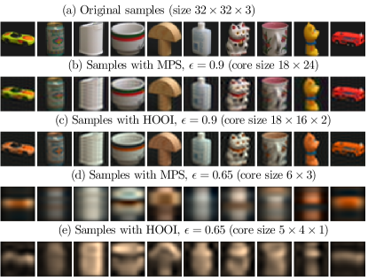
Figure 1: Modification of ten objects in the training set of COIL-100 are shown after applying MPS and HOOI corresponding to $\epsilon=0.9$ and $0.65$ to compress tensor objects.

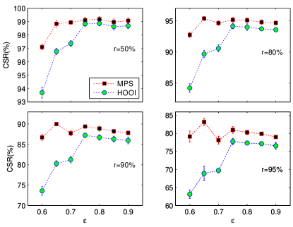
Figure 2: Error bar plots of CSR versus thresholding rate $\epsilon$ for different H/O ratios.

K nearest neighbors with K=1 (KNN-1) is used for classification. For each H/O ratio, the CSR is averaged over 10 iterations of randomly splitting the dataset into training and test sets. Comparison of performance between MPS and HOOI is shown in Fig. 2 for four different H/O ratios, i.e. $r=(50\%,80\%,90\%,95\%)$. In each plot, we show the CSR with respect to threshold $\epsilon$. We can see that MPS performs quite well when compared to HOOI. Especially, with small $\epsilon$, MPS performs much better than HOOI. Besides, we also show the best CSR corresponding to each H/O ratio obtained by different methods in Table. I. It can be seen that MPS always gives better results than HOOI even in the case of small value of $\epsilon$ and number of features $N_{f}$ defined by (10) and (19) for HOOI and MPS, respectively.

IV-B2 Extended Yale Face Database B

The EYFB dataset contains 16128 grayscale images with 28 human subjects, under 9 poses, where for each pose there is 64 illumination conditions. Similar to [29], to improve computational time each image was cropped to keep only the center area containing the face, then resized to 73 x 55. The training and test datasets are not selected randomly but partitioned according to poses. More precisely, the training and test datasets are selected to contain poses 0, 2, 4, 6 and 8 and 1, 3, 5, and 7, respectively. For a single subject the training tensor has size $5\times 73\times 55\times 64$ and $4\times 73\times 55\times 64$ is the size of the test tensor. Hence for all 28 subjects we have fourth-order tensors of sizes $140\times 73\times 55\times 64$ and $112\times 73\times 55\times 64$ for the training and test datasets, respectively.

TABLE II: EYFB classification results

Algorithm	CSR ($\epsilon=0.9$)	CSR ($\epsilon=0.85$)	CSR ($\epsilon=0.80$)	CSR ($\epsilon=0.75$)
KNN-1
HOOI	$90.71\pm 1.49$	$90.89\pm 1.60$	$91.61\pm 1.26$	$88.57\pm 0.80$
MPS	${\bf 94.29\pm 0.49}$	${\bf 94.29\pm 0.49}$	${\bf 94.29\pm 0.49}$	${\bf 94.29\pm 0.49}$
TTPCA	$86.05\pm 0.44$	$86.01\pm 0.86$	$87.33\pm 0.46$	$86.99\pm 0.53$
MPCA	$90.89\pm 1.32$
R-UMLDA	$71.34\pm 2.86$
LDA
HOOI	$96.07\pm 0.80$	$95.89\pm 0.49$	$96.07\pm 0.49$	$96.07\pm 0.49$
MPS	${\bf 97.32\pm 0.89}$	${\bf 97.32\pm 0.89}$	${\bf 97.32\pm 0.89}$	${\bf 97.32\pm 0.89}$
TTPCA	$95.15\pm 0.45$	$95.15\pm 0.45$	$95.15\pm 0.45$	$94.86\pm 0.74$
MPCA	$90.00\pm 2.92$
R-UMLDA	$73.38\pm 1.78$

TABLE III: BCI Jiaotong classification results

Algorithm	CSR ($\epsilon=0.9$)	CSR ($\epsilon=0.85$)	CSR ($\epsilon=0.80$)	CSR ($\epsilon=0.75$)
Subject 1
HOOI	$84.39\pm 1.12$	$83.37\pm 0.99$	$82.04\pm 1.05$	$84.80\pm 2.21$
MPS	${\bf 87.24\pm 1.20}$	${\bf 87.55\pm 1.48}$	${\bf 87.24\pm 1.39}$	${\bf 87.65\pm 1.58}$
TTPCA	$78.57\pm 3.95$	$78.43\pm 3.73$	${79.43\pm 4.12}$	${79.14\pm 2.78}$
MPCA	$82.14\pm 3.50$
R-UMLDA	$63.18\pm 0.37$
CSP	$80.14\pm 3.73$
Subject 2
HOOI	$83.16\pm 1.74$	$82.35\pm 1.92$	$82.55\pm 1.93$	$79.39\pm 1.62$
MPS	${\bf 90.10\pm 1.12}$	${\bf 90.10\pm 1.12}$	${\bf 90.00\pm 1.09}$	${\bf 91.02\pm 0.70}$
TTPCA	${80.57\pm 0.93}$	${81.14\pm 1.86}$	${81.29\pm 1.78}$	${80\pm 2.20}$
MPCA	$81.29\pm 0.78$
R-UMLDA	$70.06\pm 0.39$
CSP	$81.71\pm 8.96$
Subject 3
HOOI	$60.92\pm 1.83$	$61.84\pm 1.97$	$61.12\pm 1.84$	$60.51\pm 1.47$
MPS	${61.12\pm 1.36}$	${61.22\pm 1.53}$	${61.12\pm 1.54}$	${60.71\pm 1.54}$
TTPCA	${67.43\pm 2.56}$	${68.29\pm 2.56}$	${67.71\pm 2.28}$	${66.43\pm 2.02}$
MPCA	$56.14\pm 2.40$
R-UMLDA	$57.86\pm 0.00$
CSP	${\bf 77.14\pm 2.26}$
Subject 4
HOOI	$48.27\pm 1.54$	$47.55\pm 1.36$	$49.98\pm 1.29$	$47.96\pm 1.27$
MPS	${52.35\pm 2.82}$	${52.55\pm 3.40}$	${52.55\pm 3.69}$	${51.84\pm 3.11}$
TTPCA	${50.29\pm 2.97}$	${49.71\pm 3.77}$	${49.14\pm 3.48}$	${52.00\pm 3.48}$
MPCA	$51.00\pm 3.96$
R-UMLDA	$46.36\pm 0.93$
CSP	${\bf 59.86\pm 1.98}$
Subject 5
HOOI	${\bf 60.31\pm 1.08}$	${\bf 60.82\pm 0.96}$	${\bf 59.90\pm 2.20}$	${\bf 60.41\pm 1.36}$
MPS	${59.39\pm 2.08}$	${59.18\pm 2.20}$	${58.57\pm 1.60}$	${59.29\pm 1.17}$
TTPCA	${53.43\pm 2.79}$	${54.29\pm 3.19}$	${53.86\pm 3.83}$	${54.86\pm 2.49}$
MPCA	$50.43\pm 1.48$
R-UMLDA	$55.00\pm 0.55$
CSP	$59.14\pm 2.11$

TABLE IV: GAIT classification results

Algorithm	CSR ($\epsilon=0.9$)	CSR ($\epsilon=0.85$)	CSR ($\epsilon=0.80$)	CSR ($\epsilon=0.75$)
Probe A
HOOI	$63.71\pm 3.36$	$63.90\pm 3.40$	$64.16\pm 3.39$	$64.33\pm 3.20$
MPS	${70.03\pm 0.42}$	${70.03\pm 0.38}$	${70.01\pm 0.36}$	${69.99\pm 0.38}$
TTPCA	${\bf 75.31\pm 0.29}$	${\bf 76.03\pm 0.38}$	${\bf 76.38\pm 0.78}$	${\bf 77.75\pm 0.92}$
MPCA	$55.77\pm 1.08$
R-UMLDA	$46.62\pm 2.13$
Probe C
HOOI	$36.67\pm 2.84$	$36.73\pm 2.79$	$36.70\pm 3.07$	$36.87\pm 3.68$
MPS	${\bf 41.46\pm 0.64}$	${\bf 41.36\pm 0.64}$	${\bf 41.29\pm 0.63}$	${41.46\pm 0.59}$
TTPCA	${39.17\pm 0.90}$	${40.83\pm 0.41}$	${41.61\pm 1.02}$	${\bf 44.40\pm 1.54}$
MPCA	$29.35\pm 2.29$
R-UMLDA	$20.87\pm 0.76$
Probe D
HOOI	$19.73\pm 0.91$	$19.96\pm 1.15$	$20.32\pm 0.93$	$20.29\pm 1.11$
MPS	${\bf 23.82\pm 0.42}$	${\bf 23.84\pm 0.43}$	${\bf 23.84\pm 0.45}$	${\bf 23.84\pm 0.40}$
TTPCA	${21.92\pm 0.54}$	${22.14\pm 0.20}$	${22.84\pm 0.42}$	${21.92\pm 0.59}$
MPCA	$21.11\pm 3.43$
R-UMLDA	$7.88\pm 1.00$
Probe F
HOOI	${\bf 20.77\pm 0.92}$	${\bf 20.71\pm 0.72}$	$20.15\pm 0.65$	$19.96\pm 0.67$
MPS	${20.50\pm 0.40}$	${20.52\pm 0.34}$	${\bf 20.50\pm 0.29}$	${\bf 20.56\pm 0.46}$
TTPCA	${14.78\pm 0.60}$	${14.74\pm 0.77}$	${15.29\pm 0.75}$	${15.40\pm 0.55}$
MPCA	$17.12\pm 2.79$
R-UMLDA	$9.67\pm 0.58$

TABLE V: Seven experiments in the USF GAIT dataset

Probe set	A(GAL)	B(GBR)	C(GBL)	D(CAR)	E(CBR)	F(CAL)	G(CBL)
Size	71	41	41	70	44	70	44
Differences	View	Shoe	Shoe, view	Surface	Surface, shoe	Surface, view	Surface, view, shoe

In this experiment, the core tensors remains very large even with a small threshold used, e.g., for $\epsilon=0.75$, the core size of each sample obtained by TTPCA/MPS and HOOI are $18\times 201=3618$ and $14\times 15\times 13=2730$, respectively, because of slowly decaying singular values, which make them too large for classification. Therefore, we need to further reduce the sizes of core tensors before feeding them to classifiers for a better performance. In our experiment, we simply apply a further truncation to each core tensor by keeping the first few dimensions of each mode of the tensor. Intuitively, this can be done as we have already known that the space of each mode is orthogonal and ordered in such a way that the first dimension corresponds to the largest singular value, the second one corresponds to the second largest singular value and so on. Subsequently, we can independently truncate the dimension of each mode to a reasonably small value (which can be determined empirically) without changing significantly the meaning of the core tensors. It then gives rise to core tensors of smaller size that can be used directly for classification. More specifically, suppose that the core tensors obtained by MPS and HOOI have sizes $Q\times\Delta_{1}\times\Delta_{2}$ and $Q\times\Delta_{1}\times\Delta_{2}\times\Delta_{3}$, where $Q$ is the number $K$ ($L$) of training (test) samples, respectively. The core tensors are then truncated to be $Q\times\tilde{\Delta}_{1}\times\tilde{\Delta}_{2}$ and $Q\times\tilde{\Delta}_{1}\times\tilde{\Delta}_{2}\times\tilde{\Delta}_{3}$, respectively such that $\tilde{\Delta}_{l}<\Delta_{l}$ ($l=1,2,3$). Note that each $\tilde{\Delta}_{l}$ is chosen to be the same for both training and test core tensors. In regards to TTPCA, each core matrix is vectorized to have $\Delta_{1}\Delta_{2}$ features, then PCA is applied.

Classification results for different threshold values $\epsilon$ is shown in Table. II for TTPCA, MPS and HOOI using two different classifiers, i.e. KNN-1 and LDA. Results from MPCA and R-UMLDA is also included. The core tensors obtained by MPS and HOOI are reduced to have sizes of $Q\times\tilde{\Delta}_{1}\times\tilde{\Delta}_{2}$ and $Q\times\tilde{\Delta}_{1}\times\tilde{\Delta}_{2}\times\tilde{\Delta}_{3}$, respectively such that $\tilde{\Delta}_{1}=\tilde{\Delta}_{2}=\Delta\in(10,11,12,13,14)$ and $\tilde{\Delta}_{3}=1$. Therefore, the reduced core tensors obtained by both methods have the same size for classification. With MPS and HOOI, each value of CSR in Table. II is computed by taking the average of the ones obtained from classifying different reduced core tensors due to different $\Delta$. In regards to TTPCA, for each $\epsilon$, a range of principal components $p=\{50,\ldots,70\}$ is used. We utilize $Q=\{70,75,80,85,90\}$ for MPCA, and the range $m_{p}=\{10,\ldots,20\}$ for R-UMLDA. The average CSR’s are computed with TTPCA, MCPA and R-UMLDA according to their respective range of parameters in Table. II. We can see that the MPS gives rise to better results for all threshold values using different classifiers. More importantly, MPS with the smallest $\epsilon$ can produce the highest CSR. The LDA classifier gives rise to the best result, i.e. ${\bf 97.32\pm 0.89}$.

IV-B3 BCI Jiaotong

The BCIJ dataset consists of single trial recognition for BCI electroencephalogram (EEG) data involving left/right motor imagery (MI) movements. The dataset includes five subjects and the paradigm required subjects to control a cursor by imagining the movements of their right or left hand for 2 seconds with a 4 second break between trials. Subjects were required to sit and relax on a chair, looking at a computer monitor approximately 1m from the subject at eye level. For each subject, data was collected over two sessions with a 15 minute break in between. The first session contained 60 trials (30 trials for left, 30 trials for right) and were used for training. The second session consisted of 140 trials (70 trials for left, 70 trials for right). The EEG signals were sampled at 500Hz and preprocessed with a filter at 8-30Hz, hence for each subject the data consisted of a multidimensional tensor $channel\times time\times Q$. The common spatial patterns (CSP) algorithm [30] is a popular method for BCI classification that works directly on this tensor, and provides a baseline for the proposed and existing tensor-based methods. For the tensor-based methods, we preprocess the data by transforming the tensor into the time-frequency domain using complex Mortlet wavelets with bandwidth parameter $f_{b}=6$Hz (CMOR6-1) to make classification easier [31, 32]. The wavelet center frequency $f_{c}=1$Hz is chosen. Hence, the size of the concatenated tensors are $62\ channels\times 23\ frequency\ bins\times 50\ time\ frames\times Q$.

We perform the experiment for all subjects. After applying the feature extraction methods MPS and HOOI, the core tensors still have high dimension, so we need to further reduce their sizes before using them for classification. For instance, the reduced core sizes of MPS and HOOI are chosen to be $Q\times 12\times\Delta$ and $Q\times 12\times\Delta\times 1$, where $\Delta\in(8,\ldots,14)$, respectively. With TTPCA, the principal components $p=\{10,50,100,150,200\}$, $Q=\{70,75,80,85,90\}$ for MPCA and $m_{p}=\{10,\ldots,20\}$ for R-UMLDA. With CSP, we average CSR for a range of spatial components $s_{c}=\{2,4,6,8,10\}$.

The LDA classifier is utilized and the results are shown in Table. III for different threshold values of TTPCA, MPS and HOOI. The results of MPCA, R-UMLDA and CSP are also included. MPS outperforms the other methods for Subjects 1 and 2, and is comparable to HOOI in the results for Subject 5. CSP has the highest CSR for Subjects 3 and 4, followed by MPS or TTPCA, which demonstrates the proposed methods being effective at reducing tensors to relevant features, more precisely than current tensor-based methods.

Figure 3: The gait silhouette sequence for a third-order tensor.

IV-B4 USF GAIT challenge

The USFG database consists of 452 sequences from 74 subjects who walk in elliptical paths in front of a camera. There are three conditions for each subject: shoe type (two types), viewpoint (left or right), and the surface type (grass or concrete). A gallery set (training set) contains 71 subjects and there are seven types of experiments known as probe sets (test sets) that are designed for human identification. The capturing conditions for the probe sets is summarized in Table V, where G, C, A, B, L and R stand for grass surface, cement surface, shoe type A, shoe type B, left view and right view, respectively. The conditions in which the gallery set was captured is grass surface, shoe type A and right view (GAR). The subjects in the probe and gallery sets are unique and there are no common sequences between the gallery and probe sets. Each sequence is of size $128\times 88$ and the time mode is 20, hence each gait sample is a third-order tensor of size $128\times 88\times 20$, as shown in Fig. 3. The gallery set contains 731 samples, therefore the training tensor is of size $128\times 88\times 20\times 731$. The test set is of size $128\times 88\times 20\times P_{s}$, where $P_{s}$ is the sample size for the probe set that is used for a benchmark, refer to Table V. The difficulty of the classification task increases with the amount and and type of variables, e.g. Probe A only has the viewpoint, whereas Probe F has surface and viewpoint, which is more difficult. For the experiment we perform tensor object classification with Probes A, C, D and F (test sets).

The classification results based on using the LDA classifier is shown in Table IV. The threshold $\epsilon$ still retains many features in the core tensors of MPS and HOOI. Therefore, further reduction of the core tensors is chosen to be $Q\times 20\times\Delta$ and $Q\times 20\times\Delta\times 1$, where $\Delta\in(8,\ldots,14)$, respectively. The principal components for TTPCA is the range $p=\{150,200,250,300\}$, $Q=\{70,75,80,85\}$ for MPCA and $m_{p}=\{10,\ldots,20\}$ for R-UMLDA. The proposed algorithms achieve the highest performance for Probes A, C, and D. MPS and HOOI are similar for the most difficult test set Probe F.

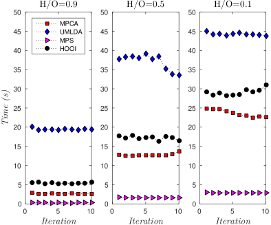
(a) COIL-100.

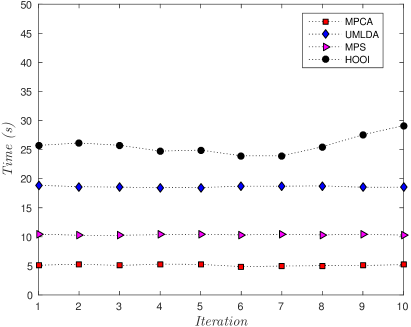
(b) EYFB.

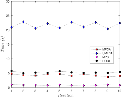
(c) BCI Subject 1.

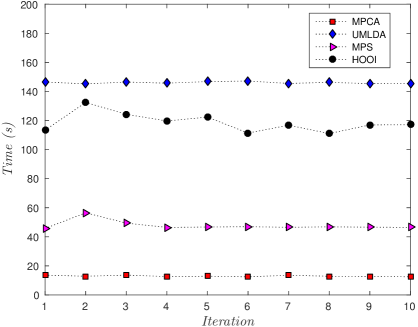
(d) GAIT Probe A.

Figure 4: Training time of datasets for MPS, MPCA, HOOI and R-UMLDA.

IV-C Training time benchmark

An additional experiment on training time for MPS, HOOI, MPCA and R-UMLDA is provided to understand the computational complexity of the algorithms. For the COIL-100 dataset, we measure the elapsed training time for the training tensor of size $32\times 32\times 3\times K$ ($K=720,3600,6480$) for H/O$=\{0.9,0.5,0.1\}$, according to 10 random partitions of train/test data (iterations). MPCA, HOOI and R-UMLDA reduces the tensor to 32 features, and MPS to 36 (due to a fixed dimension $\Delta^{2}$). In Fig. 4a, we can see that as the number of training images increases, the MPS algorithms computational time only slightly increases, while MCPA and HOOI increases gradually, with UMLDA having the slowest performance overall.

The EYFB benchmark reduces the training tensor features to 36 (for MPS), 32 (MPCA and HOOI), and 16 (UMLDA, since the elapsed time for 32 features is too long). For this case, Fig. 4b demonstrates that MPCA provides the fastest computation time due to its advantage with small sample sizes (SSS). MPS performs the next best, followed by HOOI, then UMLDA with the slowest performance.

The BCI experiment involves reducing the training tensor to 36 (MPS) or 32 (MPS, HOOI and UMLDA) features and the elapsed time is shown for Subject 1 in Fig. 4c. For this case MPS performs the quickest compared to the other algorithms, with UMLDA again performing the slowest.

Lastly, the USFG benchmark tests Probe A by reducing the MPS training tensor to 36 features, MPCA and HOOI to 32 features, and UMLDA to 16 features. Fig. 4d shows that MPCA provides the quickest time to extract the features, followed by MPS, HOOI and lastly UMLDA.

V Conclusion

In this paper, a rigorous analysis of MPS and Tucker decomposition proves the efficiency of MPS in terms of retaining relevant correlations and features, which can be used directly for tensor object classification. Subsequently, two new approaches to tensor dimensionality reduction based on compressing tensors to matrices are proposed. One method reduces a tensor to a matrix, which then utilizes PCA. And the other is a new multidimensional analogue to PCA known as MPS. Furthermore, a comprehensive discussion on the practical implementation of the MPS-based approach is provided, which emphasizes tensor mode permutation, tensor bond dimension control, and core matrix positioning. Numerical simulations demonstrates the efficiency of the MPS-based algorithms against other popular tensor algorithms for dimensionality reduction and tensor object classification.

For the future outlook, we plan to explore this approach to many other problems in multilinear data compression and tensor super-resolution.

References

• [1] H. Lu, K. N. Plataniotis, and A. N. Venetsanopoulos, “A survey of multilinear subspace learning for tensor data,” Pattern Recognition, vol. 44, no. 7, pp. 1540 – 1551, 2011.
• [2] T. G. Kolda and B. W. Bader, “Tensor decompositions and applications,” SIAM Review, vol. 51, no. 3, pp. 455–500, 2009.
• [3] L. Tucker, “Some mathematical notes on three-mode factor analysis,” Psychometrika, vol. 31, no. 3, pp. 279–311, 1966.
• [4] L. D. Lathauwer, B. D. Moor, and J. Vandewalle, “A multilinear singular value decomposition,” SIAM Journal on Matrix Analysis and Applications, vol. 21, no. 4, 2000.
• [5] M. A. O. Vasilescu and D. Terzopoulos, “Multilinear analysis of image ensembles: Tensorfaces,” Proceedings of the 7th European Conference on Computer Vision, Lecture Notes in Comput. Sci., vol. 2350, pp. 447–460, 2002.
• [6] B. Savas and L. Eldén, “Handwritten digit classification using higher order singular value decomposition,” Pattern Recognition, vol. 40, no. 3, pp. 993 – 1003, 2007.
• [7] A. H. Phan and A. Cichocki, “Tensor decompositions for feature extraction and classification of high dimensional datasets,” IEICE Nonlinear Theory and Its Applications, vol. 1, no. 1, pp. 37–68, 2010.
• [8] L. Kuang, F. Hao, L. Yang, M. Lin, C. Luo, and G. Min, “A tensor-based approach for big data representation and dimensionality reduction,” IEEE Trans. Emerging Topics in Computing, vol. 2, no. 3, pp. 280–291, Sept 2014.
• [9] A. Cichocki, D. Mandic, L. De Lathauwer, G. Zhou, Q. Zhao, C. Caiafa, and A. H. Phan, “Tensor decompositions for signal processing applications: From two-way to multiway component analysis,” IEEE Signal Processing Magazine, vol. 32, no. 2, pp. 145–163, March 2015.
• [10] L. D. Lathauwer, B. D. Moor, and J. Vandewalle, “On the best rank-1 and rank-(r1,r2,. . .,rn) approximation of higher-order tensors,” SIAM J. Matrix Anal. Appl., vol. 21, no. 4, pp. 1324–1342, Mar. 2000.
• [11] L. D. Lathauwer and J. Vandewalle, “Dimensionality reduction in higher-order signal processing and rank-(R1,R2,…,RN) reduction in multilinear algebra,” Linear Algebra and its Applications, vol. 391, no. 0, pp. 31 – 55, 2004.
• [12] H. Lu, K. Plataniotis, and A. Venetsanopoulos, “MPCA: Multilinear principal component analysis of tensor objects,” IEEE Trans. Neural Networks, vol. 19, no. 1, pp. 18–39, Jan 2008.
• [13] F. Verstraete, D. Porras, and J. I. Cirac, “Density matrix renormalization group and periodic boundary conditions: A quantum information perspective,” Phys. Rev. Lett., vol. 93, no. 22, p. 227205, Nov 2004.
• [14] G. Vidal, “Efficient classical simulation of slightly entangled quantum computation,” Phys. Rev. Lett., vol. 91, no. 14, p. 147902, Oct 2003.
• [15] ——, “Efficient simulation of one-dimensional quantum many-body systems,” Phys. Rev. Lett., vol. 93, no. 4, p. 040502, Jul 2004.
• [16] D. Pérez-García, F. Verstraete, M. Wolf, and J. Cirac, “Matrix product state representations,” Quantum Information and Computation, vol. 7, no. 5, pp. 401–430, 2007.
• [17] I. V. Oseledets, “Tensor-train decomposition,” SIAM Journal on Scientific Computing, vol. 33, no. 5, pp. 2295–2317, 2011.
• [18] J. A. Bengua, H. N. Phien, and H. D. Tuan, “Optimal feature extraction and classification of tensors via matrix product state decomposition,” in 2015 IEEE International Congress on Big Data, June 2015, pp. 669–672.
• [19] H. Lu, K. N. Plataniotis, and A. N. Venetsanopoulos, “Uncorrelated multilinear discriminant analysis with regularization and aggregation for tensor object recognition,” IEEE Transactions on Neural Networks, vol. 20, no. 1, pp. 103–123, Jan 2009.
• [20] M. Ishteva, P.-A. Absil, S. van Huffel, and L. de Lathauwer, “Best low multilinear rank approximation of higher-order tensors, based on the Riemannian trust-region scheme.” SIAM J. Matrix Anal. Appl., vol. 32, no. 1, pp. 115–135, 2011.
• [21] M. A. Nielsen and I. L. Chuang, Quantum computation and quantum information.   Cambridge, England: Cambridge University Press, 2000.
• [22] J. A. Bengua, H. N. Phien, H. D. Tuan, and M. N. Do, “Efficient tensor completion for color image and video recovery: Low-rank tensor train,” arXiv preprint, 2016. [Online]. Available: http://arxiv.org/abs/1606.01500
• [23] U. Schollwöck, “The density-matrix renormalization group in the age of matrix product states,” Annals of Physics, vol. 326, no. 1, pp. 96 – 192, 2011.
• [24] S. A. Nene, S. K. Nayar, and H. Murase, “Columbia object image library (coil-100),” Technical Report CUCS-005-96, Feb 1996.
• [25] M. Pontil and A. Verri, “Support vector machines for 3d object recognition,” IEEE Trans. Patt. Anal. and Mach. Intell., vol. 20, no. 6, pp. 637–646, Jun 1998.
• [26] A. Georghiades, P. Belhumeur, and D. Kriegman, “From few to many: illumination cone models for face recognition under variable lighting and pose,” IEEE Trans. Pattern Anal. and Mach. Intell., vol. 23, no. 6, pp. 643–660, Jun 2001.
• [27] (2013) Data set for single trial 64-channels eeg classification in bci. [Online]. Available: http://bcmi.sjtu.edu.cn/resource.html
• [28] S. Sarkar, P. J. Phillips, Z. Liu, I. R. Vega, P. Grother, and K. W. Bowyer, “The humanid gait challenge problem: data sets, performance, and analysis,” IEEE Transactions on Pattern Analysis and Machine Intelligence, vol. 27, no. 2, pp. 162–177, Feb 2005.
• [29] Q. Li and D. Schonfeld, “Multilinear discriminant analysis for higher-order tensor data classification,” IEEE Trans. Patt. Anal. and Mach. Intell., vol. 36, no. 12, pp. 2524–2537, Dec 2014.
• [30] Y. Wang, S. Gao, and X. Gao, “Common spatial pattern method for channel selelction in motor imagery based brain-computer interface,” in 2005 IEEE Engineering in Medicine and Biology 27th Annual Conference, Jan 2005, pp. 5392–5395.
• [31] Q. Zhao and L. Zhang, “Temporal and spatial features of single-trial eeg for brain-computer interface,” Computational Intelligence and Neuroscience, vol. 2007, pp. 1–14, Jun 2007.
• [32] A. H. Phan, “NFEA: Tensor toolbox for feature extraction and application,” Lab for Advanced Brain Signal Processing, BSI, RIKEN, Tech. Rep., 2011.