Majorana zero modes in spintronics devices

Abstract

We show that topological phases should be realizable in readily available and well studied heterostructures. In particular we identify a new class of topological materials which are well known in spintronics: helical ferromagnet-superconducting junctions. We note that almost all previous work on topological heterostructures has focused on creating Majorana modes at the proximity interface in effectively two-dimensional or one-dimensional systems. The particular heterostructures we address exhibit finite range proximity effects leading to nodal superconductors with Majorana modes localized well away from this interface. To show this, we implement a Bogoliubov-de Gennes (BdG) proximity numerical scheme, which importantly, involves two finite dimensions in a three dimensional junction. Incorporating this level of numerical complexity serves to distinguish ours from alternative numerical BdG approaches which are limited by generally assuming translational invariance or periodic boundary conditions along multiple directions. With this access to the edges, we are then able to illustrate in a concrete fashion the wavefunctions of Majorana zero modes, and, moreover, address finite size effects. In the process we establish consistency with a simple analytical model.

I Background

The field of topological superconductivity has generated exotic physics that realizes ideas from fields as diverse as high energy Jackiw and Rebbi (1976), atomic Xia-Ji et al. (2015); Xu and Zhang (2016); Seo et al. (2012) and condensed matter physics  Fu and Kane (2008a). Underlying this excitement has been the lofty pursuit of novel phases of matter, as well as implementing new methods for quantum computing Sau et al. (2010a). In making these superconductors experimentally there has been a central focus on materials derived from the proximity effect, where there is a higher level of experimental control. In such heterostructures, the central requirements of spin-orbit coupling Fu and Kane (2008b); Sau et al. (2010b); Linder et al. (2010); Lutchyn et al. (2010); Oreg et al. (2010), as well as a Zeeman field, and superconducting pairing can be configured artificially. For the most part these proximity-coupled exotic superconductors involve topological-insulators Fu and Kane (2008a) or semiconductors with strong spin-orbit scattering Sau et al. (2010a). In these systems, the pairing is associated with a two-dimensional (2D) $p_{x}\pm ip_{y}$ phase and under ideal circumstances this can lead to the possibilities of observing the elusive Majorana modes.

In this paper, our goal is to arrive at Majorana surface states in a different class of topological superconductors: nodal superconductors based on helical ferromagnet (F)-superconductor (S) junctions. These systems are readily available and well studied in the spintronics community Wu et al. (2012); Robinson et al. (2010); Chiodi et al. (2013). Here we characterize proximity-induced topological phases and related edge states by numerically solving the finite size Bogoliubov-de Gennes (BdG) equations and providing consistency with simple analytic arguments. The spin correlated and metallic nature of the ferromagnet results in pairing that penetrates significantly into the ferromagnetic region. This is in contrast to the focus in past topological superconductivity literature Fu and Kane (2008b); Sau et al. (2010b); Linder et al. (2010); Lutchyn et al. (2010); Oreg et al. (2010), where two or one dimensional superconductivity is proximity induced only at the interface region in insulators and semiconductors.

The resulting topological superconductivity exhibits a rich nodal structure Liu et al. (2015); Xu et al. (2015); Xu and Zhang (2016) which, importantly, is associated with the existence of one or more flat bands reflecting zero-energy surface states. We argue here these latter correspond to Majorana modes, which are found to be localized at the sample edge and outside the transition interface between the superconductor and normal phases.

Specifically we address holmium/superconductor (F/S) layered structures Wu et al. (2012); Robinson et al. (2010) which exploit the intrinsic conical order of Ho. It should be noted that there are similarities here to topological order in artificially created one- Nadj-Perge et al. (2014); Klinovaja et al. (2013); Nadj-Perge et al. (2013); Li et al. (2014) and two-dimensional spin configurations Li et al. (2016). The F/S junctions contain a host of interesting superconducting properties Sosnin et al. (2006). Among these are: (i) The presence Halterman et al. (2007, 2008); Bergeret et al. (2001) of anomalously long-range, equal-spin and $s$-wave pair correlations in the ferromagnet. (ii) The oscillatory nature of the Cooper pair amplitudes in the ferromagnetic region, which relates to Larkin-Ovchinnikov-Fulde-Ferrell (LOFF) physics Demler et al. (1997); Halterman and Valls (2001); Buzdin (2005). (iii) The observation that these triplet Cooper pairs can exist only if electrons are paired odd in time (or frequency) Bergeret et al. (2005); Volkov et al. (2006).

To incorporate these more complicated features of the F/S proximity structures into the present topological study, we introduce a BdG analysis in which there are two finite dimensions in a three dimensional system. In this way the numerics is more sophisticated than in alternative analyses Lababidi and Zhao (2011); Chiu et al. (2016) in the literature which assume periodic boundary conditions along several dimensions. As a consequence, we are able to not only demonstrate the existence of zero energy flat bands but also plot the associated Majorana wavefunctions which are localized at the edges. Importantly, these Majorana effects appear on the magnetic Ho side of a proximity junction in which there is no attractive interaction, and hence no true superconducting order parameter. We find, additionally, that ferromagnetic correlations can tunnel into the S side where there is no magnetic order parameter.

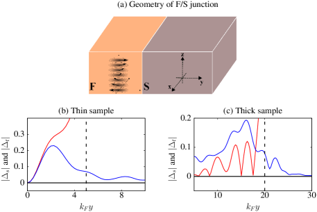
Figure 1: (a) The geometry of F/S bilayers: the interface lies on $x-z$ plane and has finite extent along the $\hat{y}$ and $\hat{z}$ directions, and is infinite in the $\hat{x}$ direction. (b) and (c) Proximity-induced singlet (red) and triplet (blue) correlations. These correlations penetrate significantly into the F (left of dashed lines) region due to the metallic structure. Panel (c) considers a thicker F region ($y=20/k_{F}$) where LOFF oscillations of the singlet component are observed, consistent with previous experiments. As shown in Panel (b) for a more narrow F region considered in this paper, no oscillations are observed.

For definiteness we show the configuration of the F/S proximity junctions in the top panel of Fig. 1. Below we present our numerical results (for two cases discussed below) for both singlet and triplet pair amplitudes. It can be seen that the singlet pair amplitudes oscillate with a much shorter decay length than their triplet counterparts. Additionally the triplet correlations, which are spread throughout the ferromagnetic side, show a small penetration into the superconducting region. These long-range triplet correlations Linder and Robinson (2015) were experimentally confirmed Robinson et al. (2010), by introducing Ho into Nb-based Josephson junctions and observing a slow decay as a function of ferromagnet thickness.

II Background theory

Our system is described by a mean-field Hamiltonian

$$\mathcal{H} = \int d^{3}\mathbf{r}\,\psi_{\sigma}^{\dagger}(\mathbf{r})\left(H_{\rm sp}+H_{\rm FM}\right)_{\sigma\sigma^{\prime}}\psi_{\sigma^{\prime}}(\mathbf{r})$$ (1)

$$+\Delta(\mathbf{r})\psi_{\uparrow}^{\dagger}(\mathbf{r})\psi_{\downarrow}^{\dagger}(\mathbf{r})+\textrm{h.c.},$$

involving fermions created (annihilated) by operators $\psi_{\sigma}^{\dagger}(\mathbf{r})$ ($\psi_{\sigma}(\mathbf{r})$) with spin $\sigma=\uparrow,\downarrow$. The single particle Hamiltonian $H_{\rm sp}=\left(-\nabla^{2}/2m-E_{F}\right)\sigma^{0}$ describes free fermions of mass $m$, and Fermi energy $E_{F}$; the identity operator $\sigma^{0}$ acts in spin space. Throughout we set $\hbar=k_{B}=1$.

The helical ferromagnet introduces a coupling term $H_{\rm FM}=\mathbf{h}({\bf r})\cdot\boldsymbol{\sigma}$, where $\boldsymbol{\sigma}=(\sigma^{x},\sigma^{y},\sigma^{z})$ is a vector of Pauli matrices operating in spin space. The conical order of the exchange field ${\mathbf{h}}$, assumed to reside only in the ferromagnet, is written as

$$\mathbf{h}=h_{0}\left\{\cos\alpha\mathbf{\hat{z}}+\sin\alpha\left[\sin\left(\frac{\beta z}{a}\right)\mathbf{\hat{x}}+\cos\left(\frac{\beta z}{a}\right)\mathbf{\hat{y}}\right]\right\},$$ (2)

where $h_{0}$ is the internal field strength of the ferromagnet. Here the helical ferromagnet parameters are set by a lattice constant along the $c$-axis of $a$, $\alpha\in[0,\pi]$ is the opening angle and $\beta$ sets the periodicity of the helix to be $\lambda=2\pi a/\beta$. The exchange field we use throughout is consistent with the parameters discussed by Chiodi et al, Chiodi et al. (2013), as is the period of the spiral order along the c-axis. While one could consider Tb or Dy de V. du Plessis et al. (1983) or even MnSi Shirane et al. (1983) which all exhibit spiral magnetism, here we focus on Ho in which the proximity effect has been more systematically established.

For notational convenience, Eq. (2) assumes a helix axis oriented along $\hat{z}$, i.e., parallel to the F/S interface as in Fig. 1; we also consider situations when this rotated by an angle $\theta\in[0,\pi]$ with respect to the $\hat{x}$-axis. While in an infinite system this axis direction is irrelevant, when finite size effects are introduced it is important as discussed below. The second line in Eq. (1) describes the pairing field $\Delta(\mathbf{r})=g(\mathbf{r})\langle\psi_{\uparrow}(\mathbf{r})\psi_{\downarrow}(\mathbf{r})\rangle$ of two fermions. This depends on the singlet pairing interaction $g(\mathbf{r})$, which is assumed to vanish in the ferromagnet and to be constant in the superconductor. Although there is no intrinsic pairing in F, a singlet pairing correlation, $\langle\psi_{\uparrow}(\mathbf{r})\psi_{\downarrow}(\mathbf{r})\rangle$ can be induced via proximity effects.

III Topological Features of Related Analytical Model

To understand possible topological phases, it is useful to first neglect the position dependence in $\Delta(\mathbf{r})$ and focus on an infinite superconductor with a uniform (non proximity induced) gap parameter $\Delta$; the magnitude of the helical ferromagnet field strength is assumed constant throughout. Applying a gauge transformation $\psi_{\uparrow}\rightarrow e^{-i\beta z/2a}\psi_{\uparrow}$ and $\psi_{\downarrow}\rightarrow e^{i\beta z/2a}\psi_{\downarrow}$, the single particle part of Eq. (1) is

$$H_{\rm sp}^{\prime}+H_{\rm FM}^{\prime}=H_{\rm sp}-v_{\rm so}\sigma^{z}i\partial_{z}+mv_{\rm so}^{2}/2+{\bf h}^{\prime}\cdot\boldsymbol{\sigma}$$ (3)

where $\mathbf{h^{\prime}}=h_{0}\left(\sin\alpha\mathbf{\hat{x}}+\cos\alpha\mathbf{\hat{z}}\right)$ and $v_{\rm so}=\beta/2ma$. In this way, the presence of helical magnetism can be viewed as imposing the important combination of a constant Zeeman field and one-dimensional spin-orbit coupling Lin et al. (2011); Martin and Morpurgo (2012); Nadj-Perge et al. (2013); Braunecker et al. (2010).

Because the gauge transformed Hamiltonian is translationally invariant, we consider the Nambu spinor $\Psi_{\mathbf{k}}=\left(\psi_{\uparrow\mathbf{k}},\psi_{\downarrow\mathbf{k}},\psi^{\dagger}_{\uparrow\mathbf{k}},\psi^{\dagger}_{\downarrow\mathbf{k}}\right)^{T},$ allowing Eq. (1) to be expressed in BdG form as $\mathcal{H}=\frac{1}{2}\sum_{\mathbf{k}}\Psi_{\mathbf{k}}^{{\dagger}}H_{\mathrm{eff}}\Psi_{\mathbf{k}}$, where

$$H_{\mathrm{eff}} = \epsilon_{\mathbf{k}}\tau^{z}-v_{\rm so}k_{z}\sigma^{z}+h_{0}\left(\cos\alpha\sigma^{z}+\sin\alpha\sigma^{x}\right)\tau^{z}$$ (4)

$$+ \Delta(i\sigma^{y})\tau^{+}+\Delta^{*}(-i\sigma^{y})\tau^{-}.$$

Here ${\bf k}=(k_{x},k_{y},k_{x})$ is a 3D momentum for a dispersion $\epsilon(\mathbf{k})=\mathbf{k}^{2}/2m-\mu$, where $E_{F}\to\mu=E_{F}-mv_{\rm so}^{2}/2$ is a renormalized chemical potential; in this work, we presume $\mu>0$ as is appropriate to F/S heterojunctions. We also define the Pauli matrices $\tau^{i}$ to operate in particle-hole space with $\tau^{\pm}=\left(\tau^{x}+i\tau^{y}\right)/2$.

The topological phase diagram is analytically tractable for the conical opening angle $\alpha=\pi/2$. In a different context, this Hamiltonian has been explored elsewhere at other opening angles Xia-Ji et al. (2015); Xu and Zhang (2016); Seo et al. (2012). The four bands of the quasi-particle energy spectrum satisfy

$$E_{\bf k}^{2}=\epsilon_{\bf k}^{2}+v_{\rm so}^{2}k_{z}^{2}+h_{0}^{2}+|\Delta|^{2}\pm 2\sqrt{\epsilon_{\bf k}^{2}\left(v_{\rm so}^{2}k_{z}^{2}+h_{0}^{2}\right)+h_{0}^{2}|\Delta|^{2}}.$$ (5)

The one-dimensionality (or “equal Rashba-Dresselhaus” limit) of the spin-orbit coupling results in a topological phase structure that is qualitatively distinct from that frequently studied in proximity systems. Rather than gapped topological phases, the above dispersion relation is associated with bulk nodal topological phases, which are characterized Seo et al. (2012); Anderson et al. (2015), by analyzing the spectrum as a function of $k_{\perp}\equiv\sqrt{k_{x}^{2}+k_{y}^{2}}$. The physics of the nodal points depends crucially on the dimension of the system, with a three-dimensional system having zero, one, or two nodal lines, while in two dimensions there are zero, two, or four Dirac points Seo et al. (2012).

It is important to establish that these topological nodal features are robust. We consider a perturbation of the form $m\tau^{i}\sigma^{j}$. As long as particle-hole symmetry $\Xi=*\tau^{x}$ (where $*$ is anti-unitary complex conjugation) and chiral symmetry $\mathcal{C}=-\tau^{y}\sigma^{x}$ are preserved, the only effect of $m$ is to renormalize $\mu,\Delta$ or $h_{0}$. Notably perturbations of this form will not introduce a gap in the system. This chiral symmetry is exact for $\alpha=\pi/2$, and therefore, in this case, the nodal structure is topologically protected.

In particular we consider the 2D limit by setting $k_{y}=0$; when $h_{0}<|\Delta|$, the system is gapped and in the trivial phase. When $|\Delta|<h_{0}<\sqrt{\mu^{2}+|\Delta|^{2}},$ the gap closes resulting in a topological phase with four Dirac points at $k_{x}^{2}=\left(k_{x}^{\pm}\right)^{2}\equiv 2m\left(\mu\pm\sqrt{h_{0}^{2}-|\Delta|^{2}}\right)$. In the strong magnetic field limit, $h_{0}>\sqrt{\mu^{2}+|\Delta|^{2}}$, the two Dirac points at $\pm k_{x}^{-}$ annihilate, resulting in two total Dirac points at $\pm k_{x}^{+}$. The boundaries of these inequalities correspond to topological phase transitions.

In a general topologically-non-trivial phase, one finds gapless surface modes Hasan and Kane (2010); Qi and Zhang (2011); specifically, for topological superconductors these are Majorana modes Majorana (1937); Beenakker (2011); Alicea (2012). To analytically establish these Majorana surface modes we demonstrate a correspondence with the well known Su-Schrieffer-Heeger (SSH) Jackiw and Rebbi (1976); Su et al. (1979) model. Without loss of generality, we take $k_{y}=0$ and look at low energy excitations around the two nodal points $\mathbf{k}^{\pm}_{c}=(\pm k_{x}^{+},0,0)$; a similar argument follows expanding around the points $\pm k_{x}^{-}$. When the system has a finite extent, these will turn out to be connected by a flat band, as in the left panel of Fig. 6. Let us expand around the nodal points $\mathbf{k}=\mathbf{k}^{\pm}_{c}+\mathbf{q}$: to first order in $\mathbf{q}$, $H_{0}(\mathbf{k})=H_{0}(\mathbf{k}_{c})+\nabla_{\mathbf{k}}H_{0}(\mathbf{k}_{c})\cdot\mathbf{q}$. The matrix $H_{0}(\mathbf{k}_{c})$ has two non-zero eigenvalues along with two vanishing eigenvalues. Projecting into the degenerate subspace of these latter two eigenvalues yields

$$\nabla_{\mathbf{k}}\bar{H}_{0}(\mathbf{k}_{c})\cdot\mathbf{q}=\pm v_{1}q_{x}\bar{\sigma}^{1}+v_{\rm so}q_{z}\bar{\sigma}^{2}$$ (6)

where $v_{1}={\Omega k_{x}^{+}}/{mh_{0}}$. Here $\Omega=\sqrt{h_{0}^{2}-\Delta^{2}}$ and the rotated Pauli matrices are given by $\bar{\sigma}^{1}=\sigma^{x}$, $\bar{\sigma}^{2}=(h_{0}\sigma^{z}+i\Omega\sigma^{y})/h_{0}$, and the two distinct signs $\pm$, reflect distinct fermion helicities. Equation (6) is evidently of the form of an effective Su-Schrieffer-Heeger Jackiw and Rebbi (1976); Su et al. (1979) Hamiltonian. In particular, here we contemplate an interface at $z=0$ separating different phases $q_{x}>0$ and $q_{x}<0$ so that this mapping establishes the existence of surface states at the $z=0$ interface. Importantly, these correspond to localized zero energy Majorana modes. When we consider an extended system along $\hat{x}$, a value of $k_{x}^{2}>0$ will drive a topological phase transition in the dimensionally reduced Hamiltonian. This results in a flat band of Majorana edge states connecting the Dirac points.

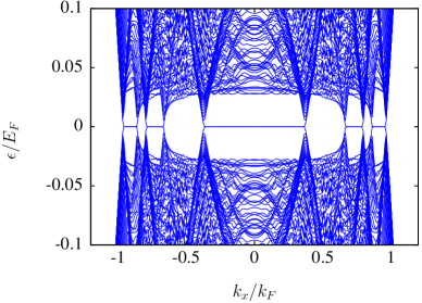
Figure 2: The dispersion relation for a thin (homogenous) topological superconductor ($k_{F}d_{y}=10$) where the exchange field strength and the pair potential are forced to be uniform throughtout the bulk. The three distinct zero-energy flat bands, and additional Dirac points, can be understood as coming from a finite-size quantization of modes along the $\hat{y}$-direction. The location of these flat bands is consistent with an analytic analysis of the BdG dispersion.

III.1 Triplet Pairing Correlations

Motivated by interest from the superconducting spintronics community, we address the triplet, time dependent correlation functions $f_{0}\left(\mathbf{r},t\right)=\left(f_{\uparrow\downarrow}\left(\mathbf{r},t\right)+f_{\uparrow\downarrow}\left(\mathbf{r},t\right)\right)/2$ and $f_{1}\left(\mathbf{r},t\right)=\left(f_{\uparrow\uparrow}\left(\mathbf{r},t\right)-f_{\downarrow\downarrow}\left(\mathbf{r},t\right)\right)/2$, where $f_{\sigma\sigma^{\prime}}\left(\mathbf{r},t\right)=\left\langle\psi_{\sigma}(\mathbf{r},t)\psi_{\sigma^{\prime}}(\mathbf{r},0)\right\rangle$. Both components can be seen to vanish at $t=0$. Using Eq. (4) one can calculate the anomalous Green’s function $F_{\sigma\sigma^{\prime}}(\omega_{n})$ as the Fourier transform of $f_{\sigma\sigma^{\prime}}(t)$, and it follows that the corresponding odd frequency pair amplitude defined through $f_{\sigma\sigma^{\prime}}^{-}(\omega_{n})\equiv\frac{1}{2}[F_{\sigma\sigma^{\prime}}(\omega_{n})-F_{\sigma\sigma^{\prime}}(-\omega_{n})]$  Ebisu et al. (2015) satisfies

$$f_{\uparrow\uparrow}^{-}=-f_{\downarrow\downarrow}^{-}=\frac{-2i\omega_{n}h_{0}\Delta}{\alpha(\omega_{n},\mathbf{k})},\ f_{\uparrow\downarrow}^{-}=f^{-}_{\downarrow\uparrow}=0$$ (7)

with $\alpha\left(\omega_{n},\mathbf{k}\right)$ even in $\mathbf{k}$ and Matsubara frequency $\omega_{n}$. In this way both the $m_{s}=1$ and $m_{s}=-1$ ($f^{-}_{\uparrow\uparrow}$ and $f^{-}_{\downarrow\downarrow}$) triplet correlations can be present while $m_{s}=0$ ($f^{-}_{\uparrow\downarrow}+f^{-}_{\downarrow\uparrow}$) is entirely absent. As a consequence, the $m_{s}=0$ component, if it is present, can only be induced near the edge, where Majorana modes appear.

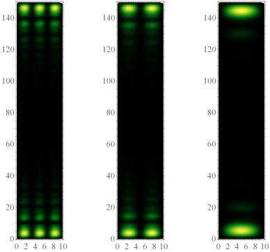
Figure 3: BdG wavefunctions of a zero energy mode for the three flat bands observed in Fig. 2. From the left to the right panel, wavefunctions belong to the zero energy band of the range $0<k_{x}<0.37$, $0.66<k_{x}<0.79$, and $0.86<k_{x}<0.96$ are plotted respectively. The number of maxima along the $\hat{y}$- directions decreases when $k_{x}$ increases, consistent with our analytic analysis.

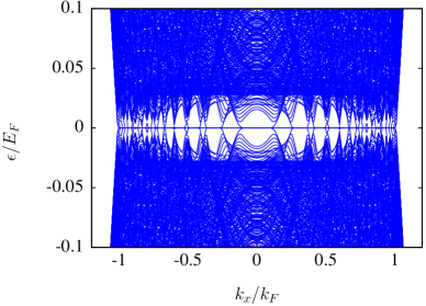
Figure 4: The BdG dispersion relation for a wider junction, where $k_{F}d_{y}=50$. The momentum modes $k_{y}=n\pi/k_{F}d_{y}$, along $\hat{y}$, are still quantized, but with spacing that is five times denser than the thin junction discussed in Fig. 2. Therefore, there are many more flat bands correspond to each $k_{y}$ than the case shown in Fig. 2. The numerous flat bands significantly overlap and approximately recover the two-dimensional flat band connecting Weyl rings for the case of a fully three-dimensional (nodal) topological superconductor. This is as would be expected from Eq. (5).

IV Numerical Study of Proximity Systems

The above mapping onto the SSH model suggests that the proximity region of a F/S heterostructure can host interesting topological phases with Majorana flat band edge states. We next confirm this by numerically implementing the counterpart proximity junction calculations using a fully self-consistent scheme which allows for a spatially inhomogeneous gap $\Delta({\bf r})$. Specifically, we consider the geometry in Fig. 1, where, importantly, the system has finite extent along the junction direction $\hat{y}$, as well as along the helical axis $\hat{z}$. We consider the $x$ direction as infinite with a momentum labeled by $k_{x}$.

The pair potential and exchange fields are functions of $y$ and $z$, and because the Hamiltonian $\mathcal{H}$ is translationally invariant along $\hat{x}$, this property allows us to write

$$u_{n\sigma}({\bf r}) =\tilde{u}_{n\sigma}({\bf r}_{\bot})e^{ik_{x}x},$$ (8)

$$v_{n\sigma}({\bf r}) =\tilde{v}_{n\sigma}({\bf r}_{\bot})e^{ik_{x}x},$$ (9)

where ${\bf r}_{\bot}=(y,z)$ and $k_{x}$ is the momentum along $\hat{x}$ direction. Then for each value of $k_{x}$, we then solve for the BdG eigenvalues and eigenfunctions

$$\begin{pmatrix}H_{\rm sp}(k_{x},{\bf r}_{\perp})+H_{\rm FM}({\bf r}_{\perp})&\Delta({\bf r}_{\perp})\left(i\sigma^{y}\right)\\ -\Delta^{*}({\bf r}_{\perp})\left(i\sigma^{y}\right)&-H_{\rm sp}^{*}(k_{x},{\bf r}_{\perp})-H_{\rm FM}^{*}({\bf r}_{\perp})\end{pmatrix}$$

$$\times\begin{pmatrix}\tilde{u}_{n\sigma}({\bf r}_{\bot})\\ \tilde{v}_{n\sigma}({\bf r}_{\bot})\end{pmatrix}=\epsilon_{n}\begin{pmatrix}\tilde{u}_{n\sigma}({\bf r}_{\bot})\\ \tilde{v}_{n\sigma}({\bf r}_{\bot})\end{pmatrix}.$$ (10)

Here, the momentum label $k_{x}$ only enters in $H_{\rm sp}(k_{x},{\bf r}_{\perp})=k_{x}^{2}/2m-\nabla^{2}_{\perp}/2m-\mu$. This acts to shift the chemical potential $\mu\rightarrow\mu-k_{x}^{2}/2m$, and in this way, the system is “dimensionally reduced” with respect to the topological properties.

The self-consistent order parameter (which depends on the interaction strength $g(\mathbf{r})$) is to be distinguished from the anomalous pairing amplitudes. The former is zero in the ferromagnet, while the latter is not. We have

$$\Delta(\mathbf{r})=g(\mathbf{r})\langle\psi_{\uparrow}(\mathbf{r})\psi_{\downarrow}(\mathbf{r})\rangle\equiv g(\mathbf{r})F(\mathbf{r})=g({\bf r}_{\bot})F({\bf r}_{\bot}).$$ (11)

We similarly define the pair amplitudes $F(\mathbf{r})\equiv\langle\psi_{\uparrow}(\mathbf{r})\psi_{\downarrow}(\mathbf{r})\rangle$.

IV.1 Introducing the Helical magnet

The exchange field $\mathbf{h}({\bf r}_{\bot})$ of the ferromagnet is given in Eq. (2), and is taken to vanish in the superconductor and to be present in the ferromagnet, so that $h_{0}({\bf r}_{\bot})=h_{0}\Theta(d_{F}-y)$. For most of this paper, the helical axis of the exchange field $\mathbf{h}$ is along the $\hat{z}$ direction. However, in experimental junctions one can contemplate a more general expression for $\mathbf{h}$ with the helical axis lying in the $y-z$ using the rotation matrix,

$$R_{x}(\theta)=\begin{pmatrix}1&0&0\\ 0&\cos\theta&\sin\theta\\ 0&-\sin\theta&\cos\theta\end{pmatrix}.$$ (12)

As a consequence the rotated exchange field $\mathbf{h}(\mathbf{r})$ is

$$\mathbf{h}(\mathbf{r})\rightarrow\mathbf{\bar{h}}(\mathbf{r})=R_{x}(\theta)\mathbf{h}\left(R_{x}^{-1}(\theta)\mathbf{r}\right).$$ (13)

The helical axis of $\mathbf{\bar{h}}(\mathbf{r})$ now makes an angle $\theta$ with respect to the $\hat{z}$-axis. This leads to

$$\bar{h}_{x} = h_{0}\sin\alpha\left[\cos\left(\frac{\beta}{a}\sin\theta y\right)\cos\left(\frac{\beta}{a}\cos\theta z\right)-\sin\left(\frac{\beta}{a}\sin\theta y\right)\sin\left(\frac{\beta}{a}\cos\theta z\right)\right],$$ (14)

$$\bar{h}_{y} = h_{0}\cos\theta\sin\alpha\left[\sin\left(\frac{\beta}{a}\sin\theta y\right)\cos\left(\frac{\beta}{a}\cos\theta z\right)+\cos\left(\frac{\beta}{a}\sin\theta y\right)\sin\left(\frac{\beta}{a}\cos\theta z\right)\right]+h_{0}\sin\theta\cos\alpha,$$ (15)

$$\bar{h}_{z} = -h_{0}\sin\theta\sin\alpha\left[\sin\left(\frac{\beta}{a}\sin\theta y\right)\cos\left(\frac{\beta}{a}\cos\theta z\right)+\cos\left(\frac{\beta}{a}\sin\theta y\right)\sin\left(\frac{\beta}{a}\cos\theta z\right)\right]+h_{0}\cos\theta\cos\alpha.$$ (16)

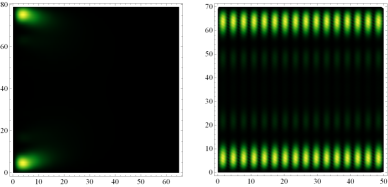
Figure 5: The BdG wavefunction of a Majorana zero mode for the (a) proximity-coupled junction and (b) a homogeneous system. (a) A calculation using the self-consistent gap in the geometry and parameters of Fig. 2(a) of the main text, with $k_{x}$ lying in the flat band. (b) The zero mode wavefunction with the gap and exchange field are forced to be homogeneous throughout the sample. This calculation helps disentangle the role of finite size effects from the inhomogeneous gap in the self-consistent calculation. Here, we take $h_{0}=0.1E_{F}$, and $k_{x}=0$ to lie in the central flat band (see also Fig. 2); all other parameters are the same as the proximity-coupled junctions. The nodal structure in the BdG wavefunction demonstrates a 3D like nature, in contrast to the quasi-2D like nature on the left panel. We find the wavenumber is approximately $k_{F}$, as is expected from the discussion of the analytic model.

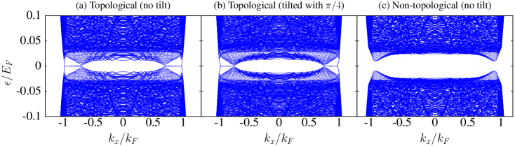
Figure 6: The dispersion of the BdG Hamiltonian (see main text) as a function of $k_{x}$ for three different helicial ferromagnets. (a) The helical axis is oriented along $\hat{z}$: zero-energy flat bands connect two pairs of topologically protected Dirac points, as predicted from the analytic model. (b) Rotating the helical axes by $\pi/4$ about the $\hat{x}$-axis, we find the Dirac cones and edge states remain. (c) With decreased ferromagnetic field strength and without rotating the axis, the system enters a trival phase.

IV.2 Numerical algorithm

We numerically solve the BdG eigenvalue problem of Eq. (10) following the scheme developed in Ref. Halterman et al. (2008). For definiteness, we set the lattice constant to be $a=k_{F}^{-1}$. We then expand both the matrix elements of Eq. (10) and the eigenfunctions in terms of a Fourier basis. For the quasi-particle and quasi-hole wavefunctions, we have

$$\tilde{u}_{n\sigma}({\bf r}_{\bot}) = \frac{2}{\sqrt{d_{y}d_{z}}}\sum_{p,q}u_{n\sigma}^{pq}\sin\left(\frac{p\pi y}{d_{y}}\right)\sin\left(\frac{q\pi z}{d_{z}}\right),$$ (17)

$$\tilde{v}_{n\sigma}({\bf r}_{\bot}) = \frac{2}{\sqrt{d_{y}d_{z}}}\sum_{p,q}v_{n\sigma}^{pq}\sin\left(\frac{p\pi y}{d_{y}}\right)\sin\left(\frac{q\pi z}{d_{z}}\right).$$ (18)

We generically define the matrix elements of an operator $M$ to be

$$M^{pqp^{\prime}q^{\prime}} \equiv \langle pq|M|p^{\prime}q^{\prime}\rangle$$ (20)

$$= \frac{4}{d_{y}d_{z}}\int_{0}^{d_{y}}\int_{0}^{d_{z}}dydz\sin\left(\frac{p\pi y}{d_{y}}\right)\sin\left(\frac{q\pi z}{d_{z}}\right)\times$$

$$\qquad M\sin\left(\frac{p^{\prime}\pi y}{d_{y}}\right)\sin\left(\frac{q^{\prime}\pi z}{d_{z}}\right).$$

Our BdG eigenvectors are then used to construct a self-consistent gap profile

$$\Delta(\mathbf{r}_{\perp})=g(\mathbf{r}_{\perp})\sum_{\epsilon_{n}<\omega_{D}}\left(u_{n\uparrow}v_{n\downarrow}^{*}-u_{n\downarrow}v_{n\uparrow}^{*}\right)\tanh(\frac{\epsilon_{n}}{2T}),$$ (21)

where the Debye frequency $\omega_{D}$ is the energy cutoff and $T$ is the temperature (we set $T=0$ in this paper). Similarly the pairing amplitudes are found to be

$$F(\mathbf{r}_{\perp})=\sum_{\epsilon_{n}<\omega_{D}}\left(u_{n\uparrow}v_{n\downarrow}^{*}-u_{n\downarrow}v_{n\uparrow}^{*}\right)\tanh(\frac{\epsilon_{n}}{2T}),$$ (22)

where the sum over the energy index $n$ also includes an integral over $k_{z}$ states. The coupling function $g({\bf r}_{\bot})=g\Theta(y-d_{F})$, where $\Theta(y)$ is the unit step function, is taken to be a constant inside the superconducting region while vanishing in the ferromagnet.

Where topological phases enter is governed by the details of the resulting energy dispersion in the Ho subsystem. These, in turn, depend on the pairing correlations. These correlations are associated with real space pairing oscillations (deriving from LOFF-like physics) and depend rather strongly on $h_{0}$. In this context, and because of the inequalities associated with topological order, the value presumed for $h_{0}$ is important, and is here taken to agree with experiment Chiodi et al. (2013). Another parameter which could be of concern is the energy cutoff $\omega_{D}$. This sets the overall superconducting transition temperatures of the pure bulk superconductor Tinkham (1996), but is otherwise irrelevant when discussing topological inequalities. For definiteness, we take $\omega_{D}=0.1E_{F}$ in all of our numerical calculations.

With this analysis, we are able to transform the inhomogenous BdG differential equation into an algebraic matrix that can be numerically diagonalized Halterman et al. (2008) to produce eigenvalues ($\epsilon_{n}$) and eigenfunctions ($u_{n}$ and $v_{n}$) thereby obtaining essentially all important quantities Halterman et al. (2008); sup .

V Finite Size Effects in Homogeneous (Non-Proximity) Superconductors

In order to calibrate the results obtained in a proximity junction, it is useful first to identify signatures of Majorana phases in a simpler situation in which a true order parameter is presumed as in the analytical model, but in a system with finite sample dimensions. This situation is more physical than in the analytically tractable model since these finite dimensions are inevitable in a proximity situation. Here, we perform a series of numerical calculations based on the assumption of a homogeneous gap taking the exchange field and the pair potential as constant. The analysis here builds on the numerical algorithm developed in the previous section, without the complexity of establishing a self-consistent spatially dependent gap. By varying the sample thickness systematically, in effect, we study a crossover of the edge mode structure from quasi-2D to 3D. Several different thicknesses $k_{F}d_{z}$ were considered, ranging from $k_{F}d_{z}=70$ to $k_{F}d_{z}=150$, and our results were found to be independent of this parameter for all the cases considered. In all calculations we assumed that the sample was infinite in the $\hat{x}$-direction.

We can more carefully map out how the system evolves by analyzing the behavior of the energy dispersion. The positive-energy branches of the continuum BdG dispersion are

$$E_{\bf k}=\sqrt{\epsilon_{\bf k}^{2}+v_{\rm so}^{2}k_{z}^{2}+h_{0}^{2}+|\Delta|^{2}\pm 2\sqrt{\epsilon_{\bf k}^{2}\left(v_{\rm so}^{2}k_{z}^{2}+h_{0}^{2}\right)+h_{0}^{2}|\Delta|^{2}}}.$$ (23)

For a 3D homogeneous and infinite sample, nodal points can only occur when $k_{z}=0$, which gives

$$E(k_{z}=0)=\sqrt{\left(k_{x}^{2}+k_{y}^{2}-1+mv_{\rm so}^{2}/2E_{F}\right)^{2}+\Delta^{2}}-h_{0},$$ (24)

where we have chosen the negative sign. For simplicity, here and in the remainder of this section, we normalize energies to $E_{F}$ and momentum to the Fermi wavevector, $k_{F}$. The correction to the chemical potential by the helical wavevector $\beta=\frac{\pi}{6a}$ is $\mu-E_{F}=mv_{\rm so}^{2}/2\approx 0.07E_{F}$ (see main text).

We consider a finite sample of width $d_{y}$ in the $\hat{y}$ direction, with $k_{y}^{\min}=\frac{\pi}{k_{F}d_{y}}$ and $k_{y}^{\max}\approx 1$. When $d_{y}$ goes to infinity, $k_{y}^{\min}$ vanishes. However, for a sufficiently small sample, the discretized nature will result in quantized momentum modes $k_{y}=\frac{n\pi}{k_{F}d_{y}}$ for integer $n$. The resulting excitation spectrum will be approximated by “cuts” through the full 3D spectrum, where $k_{y}$ is fixed. To see this, consider the spectrum when $k_{y}$ has been replaced with a quantized mode:

$$E(k_{z}=0)=\sqrt{\left(k_{x}^{2}+\left(\frac{n\pi}{k_{F}d_{y}}\right)^{2}-1+mv_{\rm so}^{2}/2E_{F}\right)^{2}+\Delta^{2}}-h_{0}.$$ (25)

This quantity vanishes when

$$k_{x}^{2}=1-mv_{\rm so}^{2}/2E_{F}-\left(\frac{n\pi}{k_{F}d_{y}}\right)^{2}\pm\sqrt{h_{0}^{2}-\Delta^{2}}.$$ (26)

is satisfied. As a result, the finite size along $d_{y}$ effectively renormalizes the chemical potential and shifts the topological phase boundary.

For the example we address below, we take $h_{0}=0.1$, $\Delta=0.032$, $k_{F}d_{y}=10$ and $k_{F}d_{z}=150.$ Thus the two nodal points occur at $k_{x}^{-}=0.86$ and $k_{x}^{+}=0.96$. The zero energy flat band in a finite-size system then lies in the range $0.86<k_{x}<0.96$. When $n=2,$ we have $0.66<k_{x}<0.79$. For $n=3,$ we have $0<k_{x}<0.37$. This analysis shows that there will be three zero energy flat bands for $n=1,2,3$. Furthermore, for each band indexed by $n$, the corresponding wavefunction amplitudes show $n$ maxima along the $\hat{y}$-direction at two edges in the $\hat{z}$-direction. This is illustrated as Fig. 3.

To understand the limit as the width $d_{y}$ tends to infinity, we take the case of a large but finite $y$-thickness ($k_{F}d_{y}=50$), as illustrated in the electronic structure in Fig. 4. One can understand the limiting case by first visualizing a Weyl annulus lying on $k_{x}-k_{y}$ plane. If one looks at the annulus along the $k_{y}-$axis, the Weyl annulus becomes a complete line. The plot in Fig. 4 should be contrasted with that in Fig. 2.

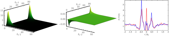
Figure 7: Plots of the (a) BdG wavefunction of the zero energy mode at $k_{x}=0.95k_{F}$ and (b) $m_{s}=0$ triplet correlations as measured by the real part of $f_{0}(t=4/\omega_{D})$ (the magnitude of the imaginary part is much smaller.) These triplet correlations cannot appear in the bulk, and only exist near the edge for both topological and trivial phases. (c) The local density of states (DOS), normalized to the DOS of the normal metal at the Fermi-level. For a thicker sample size, ($d_{z}=80/k_{F}$, red) a single zero-energy peak is observed, corresponding to localization of Majorana edge states. As the thickness is decreased ($d_{z}=30/k_{F}$, blue), the Majorana states can overlap, resuling in a splitting of the zero-energy state peak.

VI Numerical evidence for Majorana flat bands in proximity junctions

With this framework we now present numerical solutions to the BdG equations in a proximity configuration, as given in Eq. (10); this shows how Majorana modes discussed above will appear in a conical ferromagnet- superconductor junction. Unless otherwise specified, our geometry is based upon a superconducting (S) region with a coherence length $\xi=20/k_{F}$. This S region is large, with thickness (in the $\hat{y}$ direction) $60/k_{F}$, whereas we consider widths of the ferromagnet varying from $5/k_{F}$ to $20/k_{F}$. The height of the F/S junction in the $\hat{z}$-direction is $80/k_{F}$. The exchange field in Figs. 6(a) and 6(b) is $h_{0}=0.2E_{F}$.

We first observe from Figs. 1(b) and 1(c) that the pairing amplitude penetrates significantly into the F region which is to the left of the vertical dashed lines. Figure 1(b) corresponds to the case when the thickness of F is comparable to the coherence length. Here one sees that the singlet pairing amplitude exhibits oscillations of a LOFF-like form. As shown in this figure, when the oscillation length (which depends on the exchange field) is shorter than the width of the ferromagnetic region, the singlet pairing amplitude can reach zero sufficiently deep into the conical magnet. Consequently, the bulk energy spectrum is no longer fully gapped and this will destroy a topological phase.. We therefore chose the width of the F region to be large compared to the Fermi length, but still sufficiently small such that the singlet component does not assume a value of zero in the bulk. This is is the situation shown in Fig. 1(c), which is the basis for our subsequent analysis.

As a summary figure, it is useful to first to compare results for a true proximity system with one in which there is a homogeneous gap, as in the figures of the previous section. Figure 5 compares an (a) edge mode found in the proximity coupled system to (b) that of a system with a homogeneous gap throughout. In the proximity calculation, the width $k_{F}d_{y}=6$ of the ferromagnet is small compared to the correlation length, and the edge mode is tightly localized in the proximity region. In contrast, the system with a homogeneous gap has an edge mode localized through the entire region of length $k_{F}d_{y}=50$. This edge-state wavefunction has a nodal character signifying the wavefunction is a standing mode with wavevector close to $k_{F}$.

We turn to Fig. (6) which illustrates the topological structure, and emergence of Majorana flat bands in this proximity system. Just as in the analytic model of Eq. (4) there exists a critical value of $h_{0}$ that defines a transition between a fully gapped trivial phase and a topological phase with two or four Dirac points. We find that the numerically determined topological phase boundaries do not match precisely with those of the analytical model. This is presumably because there is no well defined value to assign to the parameter, $\Delta$, since the coupling $g(\mathbf{r}_{\perp})$ is zero in the ferromagnet; while there is a pairing gap which is proximity induced, it assumes a range of position dependent values.

In Fig. 6 we provide examples of the calculated energy dispersion for different orientations of the helical axis and in topological and trivial phases. As above, we fix the opening angle $\alpha=\pi/2$. The helical axes in Figs. 6(a) and 6(c) are along ${\mathbf{\hat{z}}}$, while it is along ${\mathbf{\hat{y}}}+{\mathbf{\hat{z}}}$, in Fig. 6(b). We see from the central panel that, as expected, robust Majorana phases survive up to some reasonably large rotation angle, illustrated here with $\pi/4$. For the case of a $\pi/2$ rotation additional complications, relating to LOFF oscillations ensue. By contrast, Fig. 6(c) presents the case of a smaller field strength $h_{0}=0.08E_{F}$, such that the system has crossed from the topological phase shown in the first panel, into the trivial phase. This results in a superconductor that is fully gapped without surface states.

To establish whether the zero energy flat bands of Fig. 6 are related to surface Majorana effects, in Fig. 7(a) we study the localization of the flat-band eigenfunctions in the $\hat{y}-\hat{z}$ plane. We plot these wavefunctions taking $k_{x}=0.95k_{F}$ close to a bulk nodal point; this wavefunction is localized near the $\hat{z}$-axis edge. Notably it is rather sharply peaked on the ferromagnetic side away from the precise F/S interface. This observation is what we would expect according to the analytic discussion surrounding Eq. (4). This provides some support for the conclusion that our numerical calculations have, indeed, identified Majorana modes.

Before looking for additional support, it is useful to see if these Majorana flat bands are related to the odd-frequency pairing amplitude, as has been suggested or investigated Sato et al. (2011); Black-Schaffer and Balatsky (2012); Asano and Tanaka (2013); Ebisu et al. (2015); Stanev and Galitski (2014). In Fig. 7(b), we plot the $m_{s}=0$ triplet correlation function $f_{0}$. As shown in our analytical analysis of Eq. (7) we should not find a non-vanishing $m_{s}=0$ triplet component in the bulk. This panel, indeed, shows that this particular correlation is confined to the surface, much like the Majorana modes. Notably, we find this to be the case even in the non-topological phases, so that despite the fact that they appear rather similar there is little direct correlation between the $f_{0}$ and the Majorana modes.

To establish experimental signatures for the existence of Majorana modes, we address the local density of states (LDOS) which can be probed using scanning tunneling microscopy or photoemission. Recent work Albrecht et al. (2016) exploring the nature of topological protection with end-mode separation, suggests that we analyze how a finite thickness in the $\hat{z}$ direction affects the localized nature of our flat band, zero energy modes. In the right panel of Fig. 7 we plot the LDOS for two different thicknesses. The red curve corresponds to the thicker system with $d_{z}=80/k_{F}$, where there is a single zero bias peak. For the blue curve where the thickness is substantially reduced, $d_{z}=30/k_{F}$, we find two peaks in the LDOS. This is what would be expected if the surface states were Majorana modes which had some overlap, due to finite size effects.

VII Conclusion

In this paper we have suggested a different heterostructure for readily observing nodal topological superconductivity and related Majorana surface flat bands. This is to be contrasted with the widely studied $p_{x}\pm ip_{y}$ proximity heterostructures Fu and Kane (2008a); Sau et al. (2010a) which yield a strictly two or one dimensional (gapped) topological superconductor. We consider proximity induced superconductivity in conical ferromagnets where the necessary ingredients of effective (1D) spin-orbit coupling and Zeeman fields are conveniently and simultaneously present. The feasibility of making these superconducting heterostructures is well established for Nb-Ho proximity junctions, where there is clear evidence Wu et al. (2012); Robinson et al. (2010); Linder and Robinson (2015) for finite range penetration of superconducting correlations. Here, however, we suggest that the helical axis of Ho be oriented parallel to the junction plane.

We employ a numerical Bogoliubov-de Gennes scheme which can accomodate finite length scales in two of the three dimensions. While we encounter increased numerical complexity, in contrast to periodic boundary conditions, we then have access to edges and can study the Majorana wavefunctions associated with the $E=0$ flat bands. This numerical scheme should also be compared with Eilenberger-based approaches which it was suggested Stanev and Galitski (2014) might be required in order to establish triplet, odd frequency pairing. We have demonstrated that such a pairing correlation is indeed found in our BdG approach, and is associated with the edges, rather like that of the $E=0$ Majorana states. However, because these triplet effects also appear in a non-topological phase, there is no simple correlation between the two.

We emphasize, throughout, that with our self-consistent proximity calculation, there is a clear distinction between analytical models for the equivalent topological phases (with a presumed homogeneous order parameter) and the counterpart proximity-induced phase which contains no pairing interaction and thus no order parameter in the magnetic subsystem. Nevertheless, a numerical study of a homogeneous system which includes edges and finite size effects, provides a calibration showing how Majorana flat band states will appear without proximity effects. A comparison of the wavefunction plots we find in our junctions (induced solely by proximity) provides strong support for identifying these bound surface states with Majorana flat bands.

Importantly, our calculations show that localized Majorana modes appear away from the junction interface. This presents an experimental advantage as these Majorana states are much more accessible than in a buried proximity interface. In a rather complete review of intrinsic nodal topological superfluids Schnyder and Brydon (2015) (such as high $T_{c}$ cuprates, heavy fermions and the A phase of helium-3), it was noted that the most reliable experimental signatures of Majorana flat bands involve the tunneling conductance: in particular a sharp zero bias peak. There are also weaker indications in the electromagnetic response and the anomalous spin Hall conductance and in quasi-particle interference using scanning tunneling microscopy Schnyder and Brydon (2015). Additional interest has focused on the anomalous Josephson effect Nesterov et al. (2016).

In this paper we have singled out the zero bias tunneling feature and moreover demonstrated how it is modified as the height of the junctions is reduced. This latter is suggestive of the interaction between Majorana bound states Albrecht et al. (2016) and should serve to more clearly identify these topological signatures. We observe as well, that because the Majorana modes are at the junction corner, they may be more amenable to photoemission probes.

We end by noting that we have not considered the effect of disorder in our proximity calculations, although the $s$-wave odd-frequency spin triplet state is not particularly sensitive to impurity effects, as compared with the $p$-wave even-frequency spin triplet Bergeret et al. (2005). However, even for a pristine sample, disorder is inevitable at the surface. Our numerical scheme can and will be extended to address these disorder effects in a future work.

Acknowledgements.– We thank Rufus Boyack for helpful conversations. This work was supported by NSF-DMR-MRSEC 1420709.

Appendix A Additional Numerical Details on Proximity Calculations

We present the expansion coefficients of the single particle part $H_{\mathrm{sp}}$, which can be found from explicit calculation to be

$$H_{\mathrm{sp}}^{pqp^{\prime}q^{\prime}}=\left\{\frac{1}{2m}\left[\left(\frac{p\pi}{d_{y}}\right)^{2}+\left(\frac{q\pi}{d_{z}}\right)^{2}+k_{x}^{2}\right]-E_{F}\right\}\delta_{pp^{\prime}}\delta_{qq^{\prime}}.$$ (A.1)

Similarly, the pair potential can also be expanded as $\Delta^{pqp^{\prime}q^{\prime}}\equiv\langle pq|\Delta({\bf r}_{\bot})|p^{\prime}q^{\prime}\rangle$. We also calculate the expansion coefficients for each vector component of exchange fields $h_{i}^{pp^{\prime}qq^{\prime}}$ as $\langle pq|h_{i}|p^{\prime}q^{\prime}\rangle$ $(i=x,y,z)$. for general $\theta$ defining the angle between the z direction and helical axes, we have

$$h_{x}^{pp^{\prime}qq^{\prime}} =h_{0}\sin\alpha\left(K_{1pp^{\prime}}R_{1qq^{\prime}}-K_{2pp^{\prime}}R_{2qq^{\prime}}\right),$$ (A.2)

$$h_{y}^{pp^{\prime}qq^{\prime}} =h_{0}\cos\theta\sin\alpha\left(K_{2pp^{\prime}}R_{1qq^{\prime}}+K_{1pp^{\prime}}R_{2qq^{\prime}}\right)$$ (A.3)

$$+h_{0}\sin\theta\cos\alpha D_{pp^{\prime}qq^{\prime}},$$

$$h_{z}^{pp^{\prime}qq^{\prime}} =-h_{0}\sin\theta\sin\alpha\left(K_{2pp^{\prime}}R_{1qq^{\prime}}+K_{1pp^{\prime}}R_{2qq^{\prime}}\right)$$ (A.4)

$$+h_{0}\cos\theta\cos\alpha D_{pp^{\prime}qq^{\prime}},$$

where we have defined the following quantities

$$K_{1pp^{\prime}}^{\pm\pm}= \frac{\sin\left(d_{F}\left(\frac{\beta}{a}\sin\theta\pm\frac{p\pm p^{\prime}}{d_{y}}\pi\right)\right)}{\frac{\beta}{a}\sin\theta d_{y}\pm(p\pm p^{\prime})\pi},$$

$$K_{2pp^{\prime}}^{\pm\pm}= \frac{1-\cos\left(d_{F}\left(\frac{\beta}{a}\sin\theta\pm\frac{p\pm p^{\prime}}{d_{y}}\pi\right)\right)}{\frac{\beta}{a}\sin\theta d_{y}\pm(p\pm p^{\prime})\pi},$$

$$R_{1pp^{\prime}}^{\pm\pm}= \frac{\sin\left(d_{z}\frac{\beta}{a}\cos\theta\pm\left(q\pm q^{\prime}\right)\pi\right)}{d_{z}\frac{\beta}{a}\cos\theta\pm\left(q\pm q^{\prime}\right)\pi},$$

$$R_{2pp^{\prime}}^{\pm\pm}= \frac{1-\cos\left(d_{z}\frac{\beta}{a}\cos\theta\pm\left(q\pm q^{\prime}\right)\pi\right)}{d_{z}\frac{\beta}{a}\cos\theta\pm\left(q\pm q^{\prime}\right)\pi},$$

$$D_{pp^{\prime}qq^{\prime}}= \left[\frac{\sin\left(\frac{\left(p-p^{\prime}\right)\pi d_{F}}{d_{y}}\right)}{\left(p-p^{\prime}\right)\pi}-\frac{\sin\left(\frac{\left(p+p^{\prime}\right)\pi d_{F}}{d_{y}}\right)}{\left(p+p^{\prime}\right)\pi}\right]\delta_{qq^{\prime}},$$

and

$$K_{1pp^{\prime}} = \frac{1}{2}\left(K_{1pp^{\prime}}^{+-}+K_{1pp^{\prime}}^{--}-K_{1pp^{\prime}}^{++}-K_{1pp^{\prime}}^{-+}\right),$$

$$K_{2pp^{\prime}} = \frac{1}{2}\left(K_{2pp^{\prime}}^{+-}+K_{2pp^{\prime}}^{--}-K_{2pp^{\prime}}^{++}-K_{2pp^{\prime}}^{-+}\right),$$

$$R_{1pp^{\prime}} = \frac{1}{2}\left(R_{1pp^{\prime}}^{+-}+R_{1pp^{\prime}}^{--}-R_{1pp^{\prime}}^{++}-R_{1pp^{\prime}}^{-+}\right),$$

$$R_{2pp^{\prime}} = \frac{1}{2}\left(R_{2pp^{\prime}}^{+-}+R_{2pp^{\prime}}^{--}-R_{2pp^{\prime}}^{++}-R_{2pp^{\prime}}^{-+}\right).$$

The differential BdG eigenvalue equations are now converted into algebraic eigenvalue problems. The number of terms in the Fourier series is determined through the following relations

$$\frac{1}{2m}\left(\frac{n_{y,z}^{\rm max}\pi}{d_{y,z}}\right)^{2}=E_{F}(1+\omega_{D}).$$ (A.5)

For numerical purposes, one has to use a finite number of points for the continuous variable “$k_{x}$”. We choose $k_{x}$ to be evenly distributed in the range $-k_{x}^{\rm max}<k_{x}<k_{x}^{\rm max}$, where $k_{x}^{\rm max}$ is given by

$$\frac{\left(k_{x}^{\rm max}\right)^{2}}{2m}=E_{F}(1+\omega_{D}).$$ (A.6)

We choose the number of $k_{x}$ points to be 256.

In order to find the correct energy minimum, the singlet pair amplitudes are determined self-consistently. In other words, the eigenvalue problem is solved iteratively. Once we have the self-consistent quasi-particle eigenfunctions, the triplet amplitudes can be obtained via the following equations

$$f_{0}({\bf r}_{\bot},t)$$

$$=\sum_{n}\left[u_{n\uparrow}({\bf r}_{\bot})v_{n\downarrow}^{*}({\bf r}_{\bot})+u_{n\downarrow}({\bf r}_{\bot})v_{n\uparrow}^{*}({\bf r}_{\bot})\right]\zeta_{n}(t),$$ (A.7)

$$f_{1}({\bf r}_{\bot},t)$$

$$=\sum_{n}\left[u_{n\uparrow}({\bf r}_{\bot})v_{n\uparrow}^{*}({\bf r}_{\bot})-u_{n\downarrow}({\bf r}_{\bot})v_{n\downarrow}^{*}({\bf r}_{\bot})\right]\zeta_{n}(t),$$ (A.8)

where $\zeta_{n}(t)=\cos\left(\epsilon_{n}t\right)-i\sin(\epsilon_{n}t)\tanh\left(\epsilon_{n}/2T\right)$. Another quantity discussed in the main text is the local density of states (LDOS). It is defined as

$$N_{\sigma}({\bf r}_{\bot},\epsilon)=\sum_{n}\left|u_{n\sigma}\left({\bf r}_{\bot}\right)\right|^{2}\delta(\epsilon-\epsilon_{n})+\left|v_{n\sigma}\left({\bf r}_{\bot}\right)\right|^{2}\delta(\epsilon+\epsilon_{n}),$$ (A.9)

where $\sigma=\uparrow,\downarrow$.

Appendix B Correspondence with Su-Schrieffer-Heeger Model in Case of Homogeneous Gap

Here we provide details showing the relation to the SSH model Jackiw and Rebbi (1976); Su et al. (1979).

We use an expansion around the appropriate Dirac points in the effective model to suggest the existence of protected Majorana bound states. In a topologically non-trivial phase, bulk topological signatures are associated with gapless surface modes. Specifically, we are considering a topological superconductor, where we expect the edge modes to be zero-energy Majorana states. When $h_{0}>\Delta$ and $\Omega^{2}\equiv h_{0}^{2}-\mu^{2}<\Delta^{2}$, phase transitions are signaled by a closing BdG spectral gap at $\mathbf{k}=(\pm k_{x}^{\pm},0,0)$, where

$$\frac{(k_{x}^{\pm})^{2}}{2m}-\mu=\pm\sqrt{h_{0}^{2}-|\Delta|^{2}}=\pm\Omega.$$ (B.1)

Given a momentum $k_{x}$ in a non-trivial region $k_{x}^{-}<|k_{x}|<k_{x}^{+}$, there exists a surface state associated with a flat band connecting two nodal points. We may show this explicitly by looking at low energy excitations around $k_{x}^{\pm}$.

The structure of the transition can be understood from a small-momentum expansion $\mathbf{k}=\mathbf{k}_{c}+\mathbf{q}$ around the point $\mathbf{k}_{c}=(\pm k_{x}^{+},0,0)$. To first order in $\mathbf{q}$, $H(\mathbf{k})=H(\mathbf{k}_{c})+\nabla_{\mathbf{k}}H(\mathbf{k}_{c})\cdot\mathbf{q}$ with

$$H(\mathbf{k}_{c}) = \Omega\tau^{z}+h_{0}\tau^{z}\sigma^{x}+\tau^{+}(i\sigma^{y})\Delta+\mathrm{h.c.},$$ (B.2)

$$\nabla_{\mathbf{k}}H(\mathbf{k}_{c}) = \pm\hat{\mathbf{x}}\frac{k_{x}^{+}}{m}\tau^{z}-\hat{\mathbf{z}}v_{\rm so}\sigma^{z}.,$$ (B.3)

Our BdG Hamiltonian has four distinct energy bands due to broken spin degeneracy, two are particle-like and two hole-like. The spectrum is gapless at $\mathbf{k}_{c}$ in the sense that the lower particle band and the higher hole band vanish at this point. This can be understood explicitly by diagonalizing $H(\mathbf{k}_{c})\to O^{-1}H(\mathbf{k}_{c})O$ directly at this point:

$$O^{-1}H(\mathbf{k}_{c})O=\begin{pmatrix}2h_{0}&0&0&0\\ 0&0&0&0\\ 0&0&0&0\\ 0&0&0&-2h_{0}\end{pmatrix},$$ (B.4)

where

$$O=\begin{pmatrix}\frac{h_{0}+\Omega}{\Delta}&\frac{\Omega}{\Delta}&\frac{h_{0}}{\Delta}&\frac{-h_{0}+\Omega}{\Delta}\\ \frac{h_{0}+\Omega}{\Delta}&-\frac{h_{0}}{\Delta}&-\frac{\Omega}{\Delta}&\frac{h_{0}-\Omega}{\Delta}\\ -1&0&1&1\\ 1&1&0&1\end{pmatrix}.$$ (B.5)

For notational clarity, we apply a similarity transformation using the matrices $O$ and $O^{-1}$, rather than a unitary transformation with $O$ and $O^{\dagger}$. The difference is a simple normalization of the column vectors of $O$, and the underlying physics is not affected.

It is more instructive to look at the same similarity transformation applied to $\nabla_{\mathbf{k}}H(\mathbf{k}_{c})$. We use the identities

$$O^{-1}(\tau^{z}\otimes\mathbb{I})O = \begin{pmatrix}\frac{\Omega}{h_{0}}&\frac{-h_{0}+\Omega}{2h_{0}}&\frac{h_{0}-\Omega}{2h_{0}}&0\\ -\frac{(h_{0}+\Omega)}{h_{0}}&0&\frac{\Omega}{h_{0}}&\frac{-h_{0}+\Omega}{h_{0}}\\ \frac{h_{0}+\Omega}{h_{0}}&\frac{\Omega}{h_{0}}&0&\frac{-h_{0}+\Omega}{h_{0}}\\ 0&-\frac{(h_{0}+\Omega)}{2h_{0}}&-\frac{(h_{0}+\Omega)}{h_{0}}&-\frac{\Omega}{h_{0}}\end{pmatrix}$$

$$O^{-1}(\mathbb{I}\otimes\sigma^{z})O = \begin{pmatrix}0&\frac{\Omega}{2h_{0}}&\frac{\Omega}{2h_{0}}&\frac{-h_{0}+\Omega}{h_{0}}\\ \frac{\Omega}{h_{0}}&-1&-\frac{\Omega}{h_{0}}&-\frac{\Omega}{h_{0}}\\ \frac{\Omega}{h_{0}}&\frac{\Omega}{h_{0}}&1&\frac{\Omega}{h_{0}}\\ -\frac{(h_{0}+\Omega)}{h_{0}}&-\frac{\Omega}{2h_{0}}&\frac{\Omega}{2h_{0}}&0\end{pmatrix}$$ (B.6)

The structure of the low energy surface states should follow from only the gapless bands. We therefore apply the similarity transformation $O^{-1}\nabla_{\mathbf{k}}H(\mathbf{k}_{c})O$ and extract the second and the third (gapless) bands:

$$O^{-1}(\tau^{z}\otimes\mathbb{I})O \to \frac{\Omega}{h_{0}}\begin{pmatrix}0&1\\ 1&0\end{pmatrix}=\frac{\Omega}{h_{0}}\bar{\sigma}^{x},$$ (B.7)

$$O^{-1}(\mathbb{I}\otimes\sigma^{z})O \to -\begin{pmatrix}1&0\\ 0&-1\end{pmatrix}-i\frac{\Omega}{h_{0}}\begin{pmatrix}0&-i\\ i&0\end{pmatrix},$$ (B.8)

$$= -\bar{\sigma}^{z}-i\frac{\Omega}{h_{0}}\bar{\sigma}^{y}.$$

Here we have defined new Pauli matrices $\bar{\sigma}^{i}$ that act only in the two-band low-energy subspace near the nodal points. The low-energy subspace

$$\nabla_{\mathbf{k}}H(\mathbf{k}_{c})\cdot\mathbf{q}\to q_{z}v_{\rm so}\Big{(}\bar{\sigma}^{z}+\frac{\Omega}{h_{0}}i\bar{\sigma}^{y}\Big{)}\pm\frac{\Omega k_{x}^{+}}{mh_{0}}q_{x}\bar{\sigma}^{x}.$$ (B.9)

Since $\{\bar{\sigma}^{x},\bar{\sigma}^{z}+i\bar{\sigma}^{y}\Omega/h_{0}\}=0$, after defining the constant $v_{1}=\Omega k_{x}^{+}/mh_{0}$, and the Pauli matrices $\bar{\sigma}^{1}=\bar{\sigma}^{x}$ and $\bar{\sigma}^{2}=\bar{\sigma}^{z}+i\bar{\sigma}^{y}\Omega/h_{0}$, we obtain Eq. (7) in the main text:

$$\nabla_{\mathbf{k}}\bar{H}_{0}(\mathbf{k}_{c})\cdot\mathbf{q}=\pm v_{1}q_{x}\bar{\sigma}_{1}+v_{\rm so}q_{z}\bar{\sigma}_{2}$$ (B.10)

This has the form of a Dirac Hamiltonian $q_{\mu}\gamma^{\mu}$ with $\{\gamma^{i},\gamma^{j}\}=2\delta^{ij}$.

The signature $\pm$ before $k_{x}^{+}$, corresponding to excitations near the points $\pm k^{+}_{x}$, defines distinct helicities of the excitations; thus, they are Weyl fermions. Moreover, if we regard $q_{x}$ as a parameter, i.e., applying a dimensional reduction, then the $\bar{\sigma}^{1}$ term is an effective “Dirac mass.” In this low energy effective approximation, the phase transition reflects the sign of $q_{x}$, which is associated with the sign of Dirac mass term. Breaking translational invariance in the $\hat{z}$ direction by replacing $q_{z}\to-i\partial_{z}$, we can consider an interface at $z=0$ separating inequivalent phases $q_{x}>0$ and $q_{x}^{\prime}<0.$ We have

$$H_{\mathrm{eff}}=-i\partial_{z}\gamma^{z}+M(z)\gamma^{x},$$ (B.11)

where $M$ takes the role of $v_{1}q_{x}$, and is a positive constant for $z>0$ and a negative constant for $z<0$. The Jackiw and Rebbi or the Su-Schrieffer-Heeger  Jackiw and Rebbi (1976); Su et al. (1979) story is recovered and hence we establish the bulk-edge correspondence and confirm the existence of Majorana surface states at the $z=0$ interface by solving $H_{\mathrm{eff}}\psi(z)=0.$

To be more precise, we should be able to distinguish the trivial and topological phases. If we look at $+k_{x}^{+}$ ($-k_{x}^{+}$), the Dirac mass becomes negative when $q_{x}<0$ ($q_{x}>0$). This is consistent with other analyses. On the other hand, if we expand around $\pm k_{x}^{-}$, we can again locally diagonalize $H({\bf k}_{c})$ with a different similarity matrix

$$O^{\prime}=\begin{pmatrix}\frac{h_{0}-\Omega}{\Delta}&-\frac{\Omega}{\Delta}&\frac{h_{0}}{\Delta}&-\frac{(h_{0}+\Omega)}{\Delta}\\ \frac{h_{0}-\Omega}{\Delta}&-\frac{h_{0}}{\Delta}&\frac{\Omega}{\Delta}&\frac{h_{0}+\Omega}{\Delta}\\ -1&0&1&1\\ 1&1&0&1\end{pmatrix},$$ (B.12)

which produces the similar matrices

$${O^{\prime}}^{-1}(\tau^{z}\otimes\mathbb{I})O^{\prime} = \begin{pmatrix}-\frac{\Omega}{h_{0}}&-\frac{(h_{0}+\Omega)}{2h_{0}}&\frac{h_{0}+\Omega}{2h_{0}}&0\\ \frac{-h_{0}+\Omega}{h_{0}}&0&-\frac{\Omega}{h_{0}}&-\frac{(h_{0}+\Omega)}{h_{0}}\\ \frac{h_{0}-\Omega}{h_{0}}&-\frac{\Omega}{h_{0}}&0&-\frac{(h_{0}+\Omega)}{h_{0}}\\ 0&\frac{-h_{0}+\Omega}{2h_{0}}&\frac{-h_{0}+\Omega}{h_{0}}&\frac{\Omega}{h_{0}}\end{pmatrix},$$

$${O^{\prime}}^{-1}(\mathbb{I}\otimes\sigma^{z})O^{\prime} = \begin{pmatrix}0&-\frac{\Omega}{2h_{0}}&-\frac{\Omega}{2h_{0}}&-\frac{(h_{0}+\Omega)}{h_{0}}\\ -\frac{\Omega}{h_{0}}&-1&\frac{\Omega}{h_{0}}&\frac{\Omega}{h_{0}}\\ -\frac{\Omega}{h_{0}}&-\frac{\Omega}{h_{0}}&1&-\frac{\Omega}{h_{0}}\\ \frac{-h_{0}+\Omega}{h_{0}}&\frac{\Omega}{2h_{0}}&-\frac{\Omega}{2h_{0}}&0\end{pmatrix}.$$ (B.13)

Finally, we again project into the gapless subspace, and arrive at the low-energy effective Hamiltonian

$$\nabla_{\mathbf{k}}H(\mathbf{k}_{c})\cdot\mathbf{q}\to q_{z}v_{\rm so}\left(\bar{\sigma}^{z}-\frac{\Omega}{h_{0}}i\bar{\sigma}^{y}\right)-(\pm)\frac{\Omega k_{x}^{-}}{mh_{0}}q_{x}\bar{\sigma}^{x}.$$ (B.14)

This is identical, up to signs and a replacement $k_{x}^{+}\rightarrow k_{x}^{-}$, to the effective Hamiltonian in Eq. B.9 found by expanding around the second set of Dirac points. The additional $(-1)$ appearing before $\sigma^{x}$ is necessary to make the criterion for topological phases consistent with the above arguments if we define $\gamma^{x}$ consistently.

Superficially, this approximation seems to depend on the ordering of eigenfunctions corresponding to the two gapless bands when constructing $O$ and $O^{\prime}$. However, one can show straightforwardly that such an ambiguity does not change the relevant part of $O^{-1}(\tau^{z}\otimes\mathbb{I})O$ and ${O^{\prime}}^{-1}(\tau^{z}\otimes\mathbb{I})O^{\prime}$. Our results are thus robust.

Finally, note that the topological protection is a property of the full four-band BdG Hamiltonian, and is based upon the existence of chiral symmetry. This argument does not rely on the structure of the low-energy effective expansion. Provided chiral symmetry remains, no perturbations can emerge that will result in a mass term.

References

- Jackiw and Rebbi (1976) R. Jackiw and C. Rebbi, Phys. Rev. D 13, 3398 (1976).
- Xia-Ji et al. (2015) L. Xia-Ji, H. Hui, and P. Han, Chinese Physics B 24, 050502 (2015).
- Xu and Zhang (2016) Y. Xu and C. Zhang, Phys. Rev. A 93, 063606 (2016).
- Seo et al. (2012) K. Seo, L. Han, and C. A. R. Sá de Melo, Phys. Rev. Lett. 109, 105303 (2012).
- Fu and Kane (2008a) L. Fu and C. L. Kane, Phys. Rev. Lett. 100, 096407 (2008a).
- Sau et al. (2010a) J. D. Sau, R. M. Lutchyn, S. Tewari, and S. Das Sarma, Phys. Rev. Lett. 104, 040502 (2010a).
- Fu and Kane (2008b) L. Fu and C. L. Kane, Phys. Rev. Lett. 100, 096407 (2008b).
- Sau et al. (2010b) J. D. Sau, R. M. Lutchyn, S. Tewari, and S. Das Sarma, Phys. Rev. Lett. 104, 040502 (2010b).
- Linder et al. (2010) J. Linder, Y. Tanaka, T. Yokoyama, A. Sudbø, and N. Nagaosa, Phys. Rev. Lett. 104, 067001 (2010).
- Lutchyn et al. (2010) R. M. Lutchyn, J. D. Sau, and S. Das Sarma, Phys. Rev. Lett. 105, 077001 (2010).
- Oreg et al. (2010) Y. Oreg, G. Refael, and F. von Oppen, Phys. Rev. Lett. 105, 177002 (2010).
- Wu et al. (2012) C.-T. Wu, O. T. Valls, and K. Halterman, Phys. Rev. B 86, 184517 (2012).
- Robinson et al. (2010) J. W. A. Robinson, J. D. S. Witt, and M. G. Blamire, Science 329, 59 (2010).
- Chiodi et al. (2013) F. Chiodi, J. D. S. Witt, R. G. J. Smits, L. Qu, G. B. Halasz, C.-T. Wu, O. T. Valls, K. Halterman, J. W. A. Robinson, and M. G. Blamire, EPL 101, 37002 (2013).
- Liu et al. (2015) X.-J. Liu, H. Hu, and H. Pu, Chinese Physics B 24, 050502 (2015), arXiv:1411.2993 [cond-mat.quant-gas] .
- Xu et al. (2015) Y. Xu, F. Zhang, and C. Zhang, Phys. Rev. Lett. 115, 265304 (2015).
- Nadj-Perge et al. (2014) S. Nadj-Perge, I. K. Drozdov, J. Li, H. Chen, J. Sangjun, J. Seo, A. H. MacDonald, B. Bernevig, and A. Yazdani, Science 346, 602 (2014).
- Klinovaja et al. (2013) J. Klinovaja, P. Stano, A. Yazdani, and D. Loss, Phys. Rev. Lett. 111, 186805 (2013).
- Nadj-Perge et al. (2013) S. Nadj-Perge, I. K. Drozdov, B. A. Bernevig, and A. Yazdani, Phys. Rev. B 88, 020407 (2013).
- Li et al. (2014) J. Li, H. Chen, I. K. Drozdov, A. Yazdani, B. A. Bernevig, and A. H. MacDonald, Phys. Rev. B 90, 235433 (2014).
- Li et al. (2016) J. Li, T. Neupert, Z. Wang, A. H. MacDonald, Y. Yazdani, and A. Bernevig, Nature Communications 7, 12297 (2016).
- Sosnin et al. (2006) I. Sosnin, H. Cho, V. T. Petrashov, and A. F. Volkov, Phys. Rev. Lett. 96, 157002 (2006).
- Halterman et al. (2007) K. Halterman, P. H. Barsic, and O. T. Valls, Phys. Rev. Lett. 99, 127002 (2007).
- Halterman et al. (2008) K. Halterman, O. T. Valls, and P. H. Barsic, Phys. Rev. B 77, 174511 (2008).
- Bergeret et al. (2001) F. S. Bergeret, A. F. Volkov, and K. B. Efetov, Phys. Rev. Lett. 86, 4096 (2001).
- Demler et al. (1997) E. A. Demler, G. B. Arnold, and M. R. Beasley, Phys. Rev. B 55, 15174 (1997).
- Halterman and Valls (2001) K. Halterman and O. T. Valls, Phys. Rev. B 65, 014509 (2001).
- Buzdin (2005) A. I. Buzdin, Rev. Mod. Phys. 77, 935 (2005).
- Bergeret et al. (2005) F. S. Bergeret, A. F. Volkov, and K. B. Efetov, Rev. Mod. Phys. 77, 1321 (2005).
- Volkov et al. (2006) A. F. Volkov, A. Anishchanka, and K. B. Efetov, Phys. Rev. B 73, 104412 (2006).
- Lababidi and Zhao (2011) M. Lababidi and E. Zhao, Phys. Rev. B 83, 184511 (2011).
- Chiu et al. (2016) C.-K. Chiu, W. S. Cole, and S. Das Sarma, Phys. Rev. B 94, 125304 (2016).
- Linder and Robinson (2015) J. Linder and J. W. A. Robinson, Nature Physics 11, 307 (2015).
- de V. du Plessis et al. (1983) P. de V. du Plessis, C. F. van Doorn, and D. C. van Delden, J. Magn. Magn. Mater. 40, 91 (1983).
- Shirane et al. (1983) G. Shirane, R. Cowley, C. Majkrzak, J. B. Sokoloff, B. Pagonis, C. H. Perry, and Y. Ishikawa, Phys. Rev. B 28, 6251 (1983).
- Lin et al. (2011) Y. J. Lin, K. Jimenez-Garcia, and I. B. Spielman, Nature 471, 83 (2011).
- Martin and Morpurgo (2012) I. Martin and A. F. Morpurgo, Phys. Rev. B 85, 144505 (2012).
- Braunecker et al. (2010) B. Braunecker, G. I. Japaridze, J. Klinovaja, and D. Loss, Phys. Rev. B 82, 045127 (2010).
- Anderson et al. (2015) B. M. Anderson, C.-T. Wu, R. Boyack, and K. Levin, Phys. Rev. B 92, 134523 (2015).
- Hasan and Kane (2010) M. Z. Hasan and C. L. Kane, Rev. Mod. Phys. 82, 3045 (2010).
- Qi and Zhang (2011) X.-L. Qi and S.-C. Zhang, Rev. Mod. Phys. 83, 1057 (2011).
- Majorana (1937) E. Majorana, Nuovo Cimento 14, 171 (1937).
- Beenakker (2011) C. W. J. Beenakker, ArXiv e-prints (2011), arXiv:1112.1950 [cond-mat.mes-hall] .
- Alicea (2012) J. Alicea, Reports on Progress in Physics 75, 076501 (2012).
- Su et al. (1979) W. P. Su, J. R. Schrieffer, and A. J. Heeger, Phys. Rev. Lett. 42, 1698 (1979).
- Ebisu et al. (2015) H. Ebisu, K. Yada, H. Kasai, and Y. Tanaka, Phys. Rev. B 91, 054518 (2015).
- Tinkham (1996) M. Tinkham, Introduction to Superconductivity (Dover Publications, Inc, Mineola, New York, 1996).
- (48) For details, see the Supplemental material which includes discussion of the numerical algorithm, finite size effects and the analytics underlying the Su-Schrieffer-Heeger correspondence.
- Sato et al. (2011) M. Sato, Y. Tanaka, K. Yada, and T. Yokoyama, Phys. Rev. B 83, 224511 (2011).
- Black-Schaffer and Balatsky (2012) A. M. Black-Schaffer and A. V. Balatsky, Phys. Rev. B 86, 144506 (2012).
- Asano and Tanaka (2013) Y. Asano and Y. Tanaka, Phys. Rev. B 87, 104513 (2013).
- Stanev and Galitski (2014) V. Stanev and V. Galitski, Phys. Rev. B 89, 174521 (2014).
- Albrecht et al. (2016) S. M. Albrecht, A. P. Higginbotham, M. Madsen, F. Kuenmmeth, T. S. Jespersen, J. Nygard, P. Krogstrup, and C. M. Marcus, Nature 531, 206 (2016).
- Schnyder and Brydon (2015) A. P. Schnyder and P. M. R. Brydon, Journal of Physics: Condensed Matter 27, 243201 (2015).
- Nesterov et al. (2016) K. N. Nesterov, M. Houzet, and J. S. Meyer, Phys. Rev. B 93, 174502 (2016).