Geometric control theory for quantum back-action evasion

Abstract

Engineering a sensor system for detecting an extremely tiny signal such as the gravitational-wave force is a very important subject in quantum physics. A major obstacle to this goal is that, in a simple detection setup, the measurement noise is lower bounded by the so-called standard quantum limit (SQL), which is originated from the intrinsic mechanical back-action noise. Hence, the sensor system has to be carefully engineered so that it evades the back-action noise and eventually beats the SQL. In this paper, based on the well-developed geometric control theory for classical disturbance decoupling problem, we provide a general method for designing an auxiliary (coherent feedback or direct interaction) controller for the sensor system to achieve the above-mentioned goal. This general theory is applied to a typical opto-mechanical sensor system. Also, we demonstrate a controller design for a practical situation where several experimental imperfections are present.

I Introduction

Detecting a very weak signal which is almost inaccessible within the classical (i.e., non-quantum) regime is one of the most important subjects in quantum information science. A strong motivation to devise such an ultra-precise sensor stems from the field of gravitational wave detection BraginskyBook ; Caves1980 ; Braginsky2008 ; Miao2012 ; Abbott2016 . In fact, a variety of linear sensors composed of opto-mechanical oscillators have been proposed Milburn ; Chen2013 ; Latune2013 ; Aspelmeyer2014 , and several experimental implementations of those systems in various scales have been reported Corbitt2007 ; Matsumoto2015 ; Underwood2015 ; Thompson2008 ; Verhagen2012 .

It is well known that in general a linear sensor is subjected to two types of fundamental noises, i.e., the back-action noise and the shot noise. As a consequence, the measurement noise is lower bounded by the standard quantum limit (SQL) BraginskyBook ; Caves1980 , which is mainly due to the presence of back-action noise. Hence, high-precision detection of a weak signal requires us to devise a sensor that evades the back-action noise and eventually beats the SQL; i.e., we need to have a sensor achieving back-action evasion (BAE). In fact, many BAE methods have been developed especially in the field of gravitational wave detection, e.g., the variational measurement technique Vyatchanin1995 ; Kimble2001 ; Khalili2007 or the quantum locking scheme CourtyEurophys2003 ; CourtyPhysRev2003 ; Vitali2004 . Moreover, towards more accurate detection, recently we find some high-level approaches to design a BAE sensor, based on those specific BAE methods. For instance, Ref. Miao2014 provides a systematic comparison of several BAE methods and gives an optimal solution. Also systems and control theoretical methods have been developed to synthesize a BAE sensor for a specific opto-mechanical system Tsang2010 ; YamamotoCFvsMF2014 ; in particular, the synthesis is conducted by connecting an auxiliary system to a given plant system by direct-interaction Tsang2010 or coherent feedback YamamotoCFvsMF2014 .

Along this research direction, therefore, in this paper we set the goal to develop a general systems and control theory for engineering a sensor achieving BAE, for both the coherent feedback and the direct-interaction configurations. The key tool used here is the geometric control theory Schumacher1980 ; Schumacher1982 ; Wonham1985 ; Marro2010 ; Otsuka2015 , which had been developed a long time ago. This is indeed a beautiful theory providing a variety of controller design methods for various purposes such as the non-interacting control and the disturbance decoupling problem, but, to our best knowledge, it has not been applied to problems in quantum physics. Actually in this paper we first demonstrate that the general synthesis problem of a BAE sensor can be formulated and solved within the framework of geometric control theory, particularly the above-mentioned disturbance decoupling problem.
   This paper is organized as follows. Section II is devoted to some preliminaries including a review of the geometric control theory, the general model of linear quantum systems, and the idea of BAE. Then, in Section III, we provide the general theory for designing a coherent feedback controller achieving BAE, and demonstrate an example for an opto-mechanical system. In Section IV, we discuss the case of direct interaction scheme, also based on the geometric control theory. Finally, in Section V, for a realistic opto-mechanical system subjected to a thermal environment (the perfect BAE is impossible in this case), we provide a convenient method to find an approximated BAE controller and show how much the designed controller can suppress the noise.
   Notation: For a matrix $A=(a_{ij})$, $A^{\top}$, $A^{{\dagger}}$, and $A^{\sharp}$ represent the transpose, Hermitian conjugate, and element-wise complex conjugate of $A$, respectively; i.e., $A^{\top}=(a_{ji})$, $A^{{\dagger}}=(a_{ji}^{*})$, and $A^{\sharp}=(a_{ij}^{*})=(A^{{\dagger}})^{\top}$. $\Re(a)$ and $\Im(a)$ denote the real and imaginary parts of a complex number $a$. $O$ and $I_{n}$ denote the zero matrix and the $n\times n$ identity matrix. ${\rm Ker}\hskip 1.9919ptA$ and ${\rm Im}\hskip 1.9919ptA$ denote the kernel and the image of a matrix $A$, i.e., ${\rm Ker}\hskip 1.9919ptA=\{x\,|\,Ax=0\}$ and ${\rm Im}\hskip 1.9919ptA=\{y\,|\,y=Ax,~{}\forall x\}$.

II Preliminaries

II.1 Geometric control theory for disturbance decoupling

Let us consider the following classical linear time-invariant system:

$$\frac{dx(t)}{dt} =Ax(t)+Bu(t),~{}~{}$$

$$y(t) =Cx(t)+Du(t),$$ (1)

where $x(t)\in\mathcal{X}:=\mathbb{R}^{n}$ is a vector of system variables, $u(t)\in\mathcal{U}:=\mathbb{R}^{m}$ and $y(t)\in\mathcal{Y}:=\mathbb{R}^{l}$ are vectors of input and output, respectively. $A,B,C$, and $D$ are real matrices. In the Laplace domain, the input-output relation is represented by

$$Y(s)=\Xi(s)U(s),~{}~{}\Xi(s)=C(sI-A)^{-1}B+D,$$

where $U(s)$ and $Y(s)$ are the Laplace transforms of $u(t)$ and $y(t)$, respectively. $\Xi(s)$ is called the transfer function. In this subsection, we assume $D=0$.

Now we describe the geometric control theory, for the disturbance decoupling problem Schumacher1980 ; Schumacher1982 . The following invariant subspaces play a key role in the theory.

Definition 1:  Let $A:\mathcal{X}\rightarrow\mathcal{X}$ be a linear map. Then, a subspace $\mathcal{V}\subseteq\mathcal{X}$ is said to be $A$-invariant, if $A\mathcal{V}\subseteq\mathcal{V}$.

Definition 2:  Given a linear map $A:\mathcal{X}\rightarrow\mathcal{X}$ and a subspace Im $B$ $\subseteq\mathcal{X}$, a subspace $\mathcal{V}\subseteq\mathcal{X}$ is said to be $(A,B)$-invariant, if $A\mathcal{V}\subseteq\mathcal{V}\oplus{\rm Im}\hskip 1.9919ptB$.

Definition 3:  Given a linear map $A:\mathcal{X}\rightarrow\mathcal{X}$ and a subspace Ker $C$ $\subseteq\mathcal{X}$, a subspace $\mathcal{V}\subseteq\mathcal{X}$ is said to be $(C,A)$-invariant, if $A(\mathcal{V}\cap{\rm Ker}\hskip 1.9919ptC)\subseteq\mathcal{V}$.

Definition 4:  Assume that $\mathcal{V}_{1}$ is $(C,A)$-invariant, $\mathcal{V}_{2}$ is $(A,B)$-invariant, and $\mathcal{V}_{1}\subseteq\mathcal{V}_{2}$. Then, $(\mathcal{V}_{1},\,\mathcal{V}_{2})$ is said to be a $(C,A,B)$-pair.

From Definitions 2 and 3, we have the following two lemmas.

Lemma 1:  $\mathcal{V}\subseteq\mathcal{X}$ is $(A,B)$-invariant if and only if there exists a matrix $F$ such that $F\in\mathcal{F}(\mathcal{V}):=\{F:\mathcal{X}\rightarrow\mathcal{U}\,|\,(A+BF)\mathcal{V}\subseteq\mathcal{V}\}.$

Lemma 2:  $\mathcal{V}\subseteq\mathcal{X}$ is $(C,A)$-invariant if and only if there exists a matrix $G$ such that $G\in\mathcal{G}(\mathcal{V}):=\{G:\mathcal{Y}\rightarrow\mathcal{X}\,|\,(A+GC)\mathcal{V}\subseteq\mathcal{V}\}.$

The disturbance decoupling problem is described as follows. The system of interest is represented, in an extended form of Eq. (1), as

$$\frac{dx(t)}{dt} =Ax(t)+Bu(t)+Ed(t),~{}$$

$$y(t) =Cx(t),~{}~{}z(t)=Hx(t),$$

where $d(t)$ is the disturbance and $z(t)$ is the output to be regulated. $E$ and $H$ are real matrices. The other output $y(t)$ may be used for constructing a feedback controller; see Fig. 1. The disturbance $d(t)$ can degrade the control performance evaluated on $z(t)$. Thus it is desirable if we can modify the system structure by some means so that eventually $d(t)$ dose not affect at all on $z(t)$ . This control goal is called the disturbance decoupling. Here we describe a specific feedback control method to achieve this goal; note that, as shown later, the direct-interaction method for linear quantum systems can also be described within this framework. The controller configuration is illustrated in Fig. 1; that is, the system modification is carried out by combining an auxiliary system (controller) with the original system (plant), so that the whole closed-loop system satisfies the disturbance decoupling condition. The controller with variable ${x}_{{\scriptscriptstyle K}}\in\mathcal{X}_{{\scriptscriptstyle K}}:=\mathbb{R}^{n_{\scriptscriptstyle k}}$ is assumed to take the following form:

$$\frac{dx_{{\scriptscriptstyle K}}(t)}{dt} =A_{\scriptscriptstyle K}x_{{\scriptscriptstyle K}}(t)+B_{\scriptscriptstyle K}y(t),\,$$

$$u(t) =C_{\scriptscriptstyle K}x_{{\scriptscriptstyle K}}(t)+D_{\scriptscriptstyle K}y(t),$$

where $A_{\scriptscriptstyle K}:\mathcal{X}_{{\scriptscriptstyle K}}\rightarrow\mathcal{X}_{{\scriptscriptstyle K}}$, $B_{\scriptscriptstyle K}:\mathcal{Y}\rightarrow\mathcal{X}_{{\scriptscriptstyle K}}$, $C_{\scriptscriptstyle K}:\mathcal{X}_{{\scriptscriptstyle K}}\rightarrow\mathcal{U}$, and $D_{\scriptscriptstyle K}:\mathcal{Y}\rightarrow\mathcal{U}$ are real matrices.

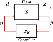
Figure 1: General configuration for the disturbance decoupling via a dynamical feedback controller.

Then, the closed-loop system defined in the augmented space $\mathcal{X}_{{\scriptscriptstyle E}}:=\mathcal{X}\oplus\mathcal{X}_{{\scriptscriptstyle K}}$ is given by

$$\frac{d}{dt}\left[\begin{array}[]{c}x\\ x_{{\scriptscriptstyle K}}\\ \end{array}\right] =\left[\begin{array}[]{cc}A+BD_{\scriptscriptstyle K}C&BC_{\scriptscriptstyle K}\\ B_{\scriptscriptstyle K}C&A_{\scriptscriptstyle K}\\ \end{array}\right]\left[\begin{array}[]{c}x\\ x_{{\scriptscriptstyle K}}\\ \end{array}\right]+\left[\begin{array}[]{c}E\\ O\\ \end{array}\right]d,~{}$$ (10)

$$z =\left[\begin{array}[]{cc}H&O\\ \end{array}\right]\left[\begin{array}[]{c}x\\ x_{{\scriptscriptstyle K}}\\ \end{array}\right].$$ (14)

The control goal is to design $(A_{\scriptscriptstyle K},B_{\scriptscriptstyle K},C_{\scriptscriptstyle K},D_{\scriptscriptstyle K})$ so that, in Eq. (10), the disturbance signal $d(t)$ dose not appear in the output $z(t)$: see the below footnote. Here, let us define

$$A_{{\scriptscriptstyle E}}=\left[\begin{array}[]{cc}A+BD_{\scriptscriptstyle K}C&BC_{\scriptscriptstyle K}\\ B_{\scriptscriptstyle K}C&A_{\scriptscriptstyle K}\\ \end{array}\right],$$ (17)

$\mathcal{B}={\rm Im}\hskip 1.9919ptB$, $\mathcal{C}={\rm Ker}\hskip 1.9919ptC$, $\mathcal{E}={\rm Im}\hskip 1.9919ptE$, and $\mathcal{H}={\rm Ker}\hskip 1.9919ptH$. Then, the following theorem gives the solvability condition for the disturbance decoupling problem.

Theorem 1:  For the closed-loop system (10), the disturbance decoupling problem via the dynamical feedback controller has a solution if and only if there exists a $(C,A,B)$-pair $(\mathcal{V}_{1},\mathcal{V}_{2})$ satisfying

$$\mathcal{E}\subseteq\mathcal{V}_{1}\subseteq\mathcal{V}_{2}\subseteq\mathcal{H}.$$ (18)

Note that this condition does not depend on the controller matrices to be designed. The following corollary can be used to check if the solvability condition is satisfied.

Corollary 1:  For the closed-loop system (10), the disturbance decoupling problem via the dynamical feedback controller has a solution if and only if

$$\mathcal{V}_{*}{\scriptscriptstyle(\mathcal{C},\mathcal{E})}\subseteq\mathcal{V}^{*}{\scriptscriptstyle(\mathcal{B},\mathcal{H})},$$

where $\mathcal{V}^{*}{\scriptscriptstyle(\mathcal{B},\mathcal{H})}$ is the maximum element of $(A,B)$-invariant subspaces contained in $\mathcal{H}$, and $\mathcal{V}_{*}{\scriptscriptstyle(\mathcal{C},\mathcal{E})}$ is the minimum element of $(C,A)$-invariant subspaces containing $\mathcal{E}$. These subspaces can be computed by the algorithms given in Appendix A.

Once the solvability condition described above is satisfied, then we can explicitly construct the controller matrices $(A_{\scriptscriptstyle K},B_{\scriptscriptstyle K},C_{\scriptscriptstyle K},D_{\scriptscriptstyle K})$. The following intersection and projection subspaces play a key role for this purpose; that is, for a subspace $\mathcal{V}_{{\scriptscriptstyle E}}\subseteq\mathcal{X}_{{\scriptscriptstyle E}}=\mathcal{X}\oplus\mathcal{X}_{{\scriptscriptstyle K}}$, let us define

$$\mathcal{V}_{{\scriptscriptstyle I}}: =\left\{x\in\mathcal{X}~{}\Bigg{|}\left[\begin{array}[]{c}x\\ O\\ \end{array}\right]\in\mathcal{V}_{{\scriptscriptstyle E}}\right\},~{}$$

$$\mathcal{V}_{{\scriptscriptstyle P}}: =\left\{x\in\mathcal{X}~{}\Bigg{|}\left[\begin{array}[]{c}x\\ x_{{\scriptscriptstyle K}}\\ \end{array}\right]\in\mathcal{V}_{{\scriptscriptstyle E}},~{}\exists{x}_{{\scriptscriptstyle K}}\in\mathcal{X}_{{\scriptscriptstyle K}}\right\}.$$

Then, the following theorem is obtained:

Theorem 2:  Suppose that $(\mathcal{V}_{1},\mathcal{V}_{2})$ is a $(C,A,B)$-pair. Then, there exist $F\in\mathcal{F}(\mathcal{V}_{2})$, $G\in\mathcal{G}(\mathcal{V}_{1})$, and $D_{\scriptscriptstyle K}:\mathcal{Y}\rightarrow\mathcal{U}$ such that ${\rm Ker}\hskip 1.9919ptF_{0}\supseteq\mathcal{V}_{1}$ and ${\rm Im}\hskip 1.9919ptG_{0}\subseteq\mathcal{V}_{2}$ hold, where $F_{0}=F-D_{\scriptscriptstyle K}C,~{}G_{0}=G-BD_{\scriptscriptstyle K}$.

Moreover, there exists $\mathcal{X}_{{\scriptscriptstyle K}}$ with ${\rm dim}\,\mathcal{X}_{{\scriptscriptstyle K}}={\rm dim}\,\mathcal{V}_{2}-{\rm dim}\,\mathcal{V}_{1}$, and $A_{{\scriptscriptstyle E}}$ has an invariant subspace $\mathcal{V}_{{\scriptscriptstyle E}}\subseteq\mathcal{X}_{{\scriptscriptstyle E}}$ such that $\mathcal{V}_{1}=\mathcal{V}_{{\scriptscriptstyle I}}$ and $\mathcal{V}_{2}=\mathcal{V}_{{\scriptscriptstyle P}}$. Also, $(A_{\scriptscriptstyle K},B_{\scriptscriptstyle K},C_{\scriptscriptstyle K})$ satisfies

$$C_{\scriptscriptstyle K}N=F_{0},~{}~{}$$

$$B_{\scriptscriptstyle K}=-NG_{0},~{}~{}$$

$$A_{\scriptscriptstyle K}N=N(A+BF_{0}+GC),$$ (19)

where $N:\mathcal{V}_{2}\rightarrow\mathcal{X}_{{\scriptscriptstyle K}}$ is a linear map satisfying ${\rm Ker}\hskip 1.9919ptN=\mathcal{V}_{1}$.

In fact, under the condition given in Theorem 2, let us define the following augmented subspace $\mathcal{V}_{{\scriptscriptstyle E}}\subseteq\mathcal{X}_{{\scriptscriptstyle E}}$:

$$\mathcal{V}_{{\scriptscriptstyle E}}:= \left\{\left[\begin{array}[]{c}x\\ Nx\\ \end{array}\right]\Bigg{|}~{}x\in\mathcal{V}_{2}\right\}.$$

Then, $\mathcal{V}_{1}=\mathcal{V}_{{\scriptscriptstyle I}}$ and $\mathcal{V}_{2}=\mathcal{V}_{{\scriptscriptstyle P}}$ hold, and we have

$$A_{{\scriptscriptstyle E}}\left[\begin{array}[]{c}x\\ Nx\\ \end{array}\right] =\left[\begin{array}[]{cc}A+BD_{\scriptscriptstyle K}C&BC_{\scriptscriptstyle K}\\ B_{\scriptscriptstyle K}C&A_{\scriptscriptstyle K}\\ \end{array}\right]\left[\begin{array}[]{c}x\\ Nx\\ \end{array}\right]$$

$$=\left[\begin{array}[]{c}(A+BF)x\\ N(A+BF)x\\ \end{array}\right]\in\mathcal{V}_{{\scriptscriptstyle E}},$$

implying that $\mathcal{V}_{{\scriptscriptstyle E}}$ is actually $A_{{\scriptscriptstyle E}}$-invariant. Now suppose that Theorem 1 holds, and let us take the $(C,A,B)$-pair $(\mathcal{V}_{1},\mathcal{V}_{2})$ satisfying Eq. (18). Then, together with the above result ($A_{{\scriptscriptstyle E}}\mathcal{V}_{{\scriptscriptstyle E}}\subseteq\mathcal{V}_{{\scriptscriptstyle E}}$), we have ${\rm Im}\hskip 1.9919pt[E^{\top}~{}O]^{\top}\subseteq\mathcal{V}_{{\scriptscriptstyle E}}\subseteq{\rm Ker}\hskip 1.9919pt[H~{}O]$. This implies that $d(t)$ must be contained in the unobservable subspace with respect to $z(t)$, and thus the disturbance decoupling is realized.

II.2 Linear quantum systems

Here we describe a general linear quantum system composed of $n$ bosonic subsystems. The $j$-th mode can be modeled as a harmonic oscillator with the canonical conjugate pairs (or quadratures) $\hat{q}_{j}$ and $\hat{p}_{j}$ satisfying the canonical commutation relation (CCR) $\hat{q}_{j}\hat{p}_{k}-\hat{p}_{k}\hat{q}_{j}=i\delta_{jk}$. Let us define the vector of quadratures as $\hat{x}=[\hat{q}_{1},\hat{p}_{1},\ldots,\hat{q}_{n},\hat{p}_{n}]^{\top}$. Then, the CCRs are summarized as

$$\hat{x}\hat{x}^{\top}-(\hat{x}\hat{x}^{\top})^{\top}=i\Sigma_{n},~{}~{}$$

$$\Sigma_{n}={\rm diag}\{\Sigma,\ldots,\Sigma\},~{}~{}~{}\Sigma=\left[\begin{array}[]{cc}0&1\\ -1&0\\ \end{array}\right].$$

Note that $\Sigma_{n}$ is a $2n\times 2n$ block diagonal matrix. The linear quantum system is an open system coupled to $m$ environment fields via the interaction Hamiltonian $\hat{H}_{\rm int}=i\sum_{j=1}^{m}(\hat{L}_{j}\hat{A}_{j}^{*}-\hat{L}_{j}^{*}\hat{A}_{j})$, where $\hat{A}_{j}(t)$ is the field annihilation operator satisfying $\hat{A}_{j}(t)\hat{A}_{k}^{*}(t^{\prime})-\hat{A}_{k}^{*}(t^{\prime})\hat{A}_{j}(t)=\delta_{jk}\delta(t-t^{\prime})$. Also $\hat{L}_{j}$ is given by $\hat{L}_{j}=c_{j}^{\top}\hat{x}$ with $c_{j}\in{\mathbb{C}}^{2n}$. In addition, the system is driven by the Hamiltonian $\hat{H}=\hat{x}^{\top}R\hat{x}/2$ with $R=R^{\top}\in\mathbb{R}^{2n\times 2n}$. Then, the Heisenberg equation of $\hat{x}$ is given by

$$\frac{d\hat{x}(t)}{dt}=A\hat{x}(t)+\sum_{j=1}^{m}B_{j}\hat{W}_{j}(t),$$ (20)

where $\hat{W}_{j}(t)$ is defined by

$$\hat{W}_{j}=\left[\begin{array}[]{cc}\hat{Q}_{j}\\ \hat{P}_{j}\\ \end{array}\right]=\left[\begin{array}[]{cc}(\hat{A}_{j}+\hat{A}_{j}^{*})/\sqrt{2}\\ (\hat{A}_{j}-\hat{A}_{j}^{*})/\sqrt{2}i\\ \end{array}\right].$$

The matrices are given by $A=\Sigma_{n}(R+\sum_{j=1}^{m}C_{j}^{\top}\Sigma C_{j}/2)$ and $B_{j}=\Sigma_{n}C_{j}^{\top}\Sigma$ with $C_{j}=\sqrt{2}[\Re(c_{j}),\Im(c_{j})]^{\top}\in\mathbb{R}^{2\times 2n}$. Also, the instantaneous change of the field operator $\hat{W}_{j}(t)$ via the system-field coupling is given by

$$\hat{W}_{j}^{\rm out}(t)=C_{j}\hat{x}(t)+\hat{W}_{j}(t).$$ (21)

Summarizing, the linear quantum system is characterized by the dynamics (20) and the output (21), which are exactly of the same form as those in Eq. (1) ($l=m$ in this case). However note that the system matrices have to satisfy the above-described special structure, which is equivalently converted to the following physical realizability condition James2008 :

$$A\Sigma_{n}+\Sigma_{n}A^{\top}+\sum_{j=1}^{m}B_{j}\Sigma B_{j}^{\top}=O,~{}B_{j}=\Sigma_{n}C_{j}^{\top}\Sigma.$$ (22)

II.3 Weak signal sensing, SQL, and BAE

The opto-mechanical oscillator illustrated in Fig. 2 is a linear quantum system, which serves as a sensor for a very weak signal. Let $\hat{q}_{1}$ and $\hat{p}_{1}$ be the oscillator’s position and momentum operators, and $\hat{a}_{2}=(\hat{q}_{2}+i\hat{p}_{2})/\sqrt{2}$ represents the annihilation operator of the cavity mode. The system Hamiltonian is given by $\hat{H}=\omega_{\scriptscriptstyle m}(\hat{q}_{1}^{2}+\hat{p}_{1}^{2})/2-g\hat{q}_{1}\hat{q}_{2}$; that is, the oscillator’s free evolution with resonant frequency $\omega_{\scriptscriptstyle m}$ plus the linearized radiation pressure interaction between the oscillator and the cavity field with coupling strength $g$.

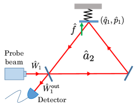
Figure 2: Opto-mechanical system for weak signal sensing.

The system couples to an external probe field (thus $m=1$) via the coupling operator $\hat{L}_{1}=\sqrt{\kappa}\hat{a}_{2}$, with $\kappa$ the coupling constant between the cavity and probe fields. The corresponding matrix $R$ and vector $c_{1}$ are then given by

$$R=\left[\begin{array}[]{cccc}\omega_{\scriptscriptstyle m}&0&-g&0\\ 0&\omega_{\scriptscriptstyle m}&0&0\\ -g&0&0&0\\ 0&0&0&0\\ \end{array}\right],~{}~{}c_{1}=\sqrt{\frac{\kappa}{2}}\left[\begin{array}[]{c}0\\ 0\\ 1\\ i\\ \end{array}\right].$$

The oscillator is driven by an unknown force $\hat{f}(t)$ with coupling constant $\gamma$ ; then the vector of system variables $\hat{x}=[\hat{q}_{1},\hat{p}_{1},\hat{q}_{2},\hat{p}_{2}]^{\top}$ satisfies

$$\frac{d\hat{x}}{dt}=A\hat{x}+B_{1}\hat{W}_{1}+b\hat{f},~{}~{}\hat{W}_{1}^{\rm out}=C_{1}\hat{x}+\hat{W}_{1},$$

where

$$A =\left[\begin{array}[]{cccc}0&\omega_{\scriptscriptstyle m}&0&0\\ -\omega_{\scriptscriptstyle m}&0&g&0\\ 0&0&-\kappa/2&0\\ g&0&0&-\kappa/2\\ \end{array}\right],\,b=\sqrt{\gamma}\left[\begin{array}[]{c}0\\ 1\\ 0\\ 0\\ \end{array}\right],$$ (31)

$$C_{1} =-B_{1}^{\top}=\left[\begin{array}[]{cccc}0&0&\sqrt{\kappa}&0\\ 0&0&0&\sqrt{\kappa}\\ \end{array}\right],$$ (34)

$$\hat{W}_{1} =[\hat{Q}_{1},\hat{P}_{1}]^{\top},~{}~{}\hat{W}_{1}^{\rm out}=[\hat{Q}_{1}^{\rm out},\hat{P}_{1}^{\rm out}]^{\top}.$$ (35)

Note that we are in the rotating frame at the frequency of the probe field. These equations indicate that the information about $\hat{f}$ can be extracted by measuring $\hat{P}_{1}^{\rm out}$ by a homodyne detector. Actually the measurement output in the Laplace domain is given by

$$\hat{P}_{1}^{\rm out}(s)=\Xi_{f}(s)\hat{f}(s)+\Xi_{Q}(s)\hat{Q}_{1}(s)+\Xi_{P}(s)\hat{P}_{1}(s),$$ (36)

where $\Xi_{f}$, $\Xi_{Q}$, and $\Xi_{P}$ are transfer functions given by

$$\Xi_{f}(s) =\frac{g\omega_{\scriptscriptstyle m}\sqrt{\gamma\kappa}}{(s^{2}+\omega_{\scriptscriptstyle m}^{2})(s+\kappa/2)},~{}~{}$$

$$\Xi_{Q}(s) =-\frac{g^{2}\omega_{\scriptscriptstyle m}\kappa}{(s^{2}+\omega_{\scriptscriptstyle m}^{2})(s+\kappa/2)^{2}},~{}~{}\Xi_{P}(s)=\frac{s-\kappa/2}{s+\kappa/2}.$$

Thus, $\hat{P}_{1}^{\rm out}$ certainly contains $\hat{f}$. Note however that it is subjected to two noises. The first one, $\hat{Q}_{1}$, is the back-action noise, which is due to the interaction between the oscillator and the cavity. The second one, $\hat{P}_{1}$, is the shot noise, which inevitably appears. Now, the normalized output is given by

$$y_{1}(s)=\frac{\hat{P}_{1}^{\rm out}(s)}{\Xi_{f}(s)}=\hat{f}(s)+\frac{\Xi_{Q}(s)}{\Xi_{f}(s)}\hat{Q}_{1}(s)+\frac{\Xi_{P}(s)}{\Xi_{f}(s)}\hat{P}_{1}(s),$$

and the normalized noise power spectral density of $y_{1}$ in the Fourier domain $(s=i\omega)$ is calculated as follows:

$$S(\omega)=\langle|y_{1}-\hat{f}|^{2}\rangle=\left|\frac{\Xi_{Q}}{\Xi_{f}}\right|^{2}\langle|\hat{Q}_{1}|^{2}\rangle+\left|\frac{\Xi_{P}}{\Xi_{f}}\right|^{2}\langle|\hat{P}_{1}|^{2}\rangle$$

$$\geq 2\sqrt{\frac{|\Xi_{Q}|^{2}|\Xi_{P}|^{2}}{|\Xi_{f}|^{4}}\langle|\hat{Q}_{1}|^{2}\rangle\langle|\hat{P}_{1}|^{2}\rangle}\geq\frac{|\omega^{2}-\omega_{\scriptscriptstyle m}^{2}|}{\gamma\omega_{\scriptscriptstyle m}}=S_{\scriptscriptstyle\rm SQL}(\omega).$$

The lower bound is called the SQL. Note that the last inequality is due to the Heisenberg uncertainty relation of the normalized noise power, i.e., $\langle|\hat{Q}_{1}|^{2}\rangle\langle|\hat{P}_{1}|^{2}\rangle\geq 1/4$. Hence, the essential reason why SQL appears is that $\hat{P}_{1}^{\rm out}$ contains both the back-action noise $\hat{Q}_{1}$ and the shot noise $\hat{P}_{1}$. Therefore, toward the high-precision detection of $\hat{f}$, we need BAE; that is, the system structure should be modified by some means so that the back-action noise is completely evaded in the output signal (note that the shot noise can never be evaded). The condition for BAE can be expressed in terms of the transfer function as follows Tsang2010 ; YamamotoCFvsMF2014 ; i.e., for the modified (controlled) sensor, the transfer function from the back-action noise to the measurement output must satisfy

$$\Xi_{Q}(s)=0,~{}~{}~{}\forall s.$$ (37)

Equivalently, $\hat{P}_{1}^{\rm out}$ contains only the shot noise $\hat{P}_{1}$; hence, in this case the signal to noise ratio can be further improved by injecting a $\hat{P}_{1}$-squeezed (meaning $\langle|\hat{P}_{1}|^{2}\rangle<1/2$) probe field into the system.

III Coherent feedback control for back-action evasion

III.1 Coherent and measurement-based feedback control

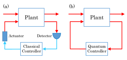
Figure 3: General configurations of feedback control for a given plant quantum system: (a) measurement-based feedback and (b) coherent feedback.

There are two schemes for controlling a quantum system via feedback. The first one is the measurement-based feedback Belavkin1999 ; Bouten2009 ; WisemanBook ; KurtBook illustrated in Fig. 3 (a). In this scheme, we measure the output fields and feed the measurement results back to control the plant system. On the other hand, in the coherent feedback scheme James2008 ; Wiseman1994 ; Yanagisawa-2003 ; Mabuchi2008 ; Iida2012 shown in Fig. 3 (b), the feedback loop dose not contain any measurement component and the plant system is controlled by another quantum system. Recently we find several works comparing the performance of these two schemes Wiseman1994 ; NurdinLQG2009 ; Hamerly2012 ; Jacobs2014 ; Devoret2016 . In particular, it was shown in YamamotoCFvsMF2014 that there are some control tasks that cannot be achieved by any measurement-based feedback but can be done by a coherent one. More specifically, those tasks are realizing BAE measurement, generating a quantum non-demolished variable, and generating a decoherence-free subsystem; in our case, of course, the first one is crucial. Hence, here we aim to develop a theory for designing a coherent feedback controller such that the whole controlled system accomplishes BAE.

III.2 Coherent feedback for BAE

As discussed in Section II.1, the geometric control theory for disturbance decoupling problem is formulated for the controlled system with special structure (10); in particular, the coefficient matrix of the disturbance $d(t)$ is of the form $[E^{\top},O]^{\top}$ and that of the state vector in the output $z(t)$ is $[H,O]$. Here we consider a class of coherent feedback configuration such that the whole closed-loop system dynamics has this structure, in order for the geometric control theory to be directly applicable.

First, for the plant system given by Eqs. (20) and (21), we assume that the system couples to all the probe fields in the same way; i.e.,

$$B_{j}=B~{}~{}~{}\forall j.$$ (38)

This immediately leads to $C_{j}=C~{}\forall j$. Next, as the controller, we take the following special linear quantum system with $(m-1)$ input-output fields:

$$\frac{d\hat{x}_{\scriptscriptstyle K}}{dt} =A_{\scriptscriptstyle K}\hat{x}_{\scriptscriptstyle K}+\sum_{j=1}^{m-1}B_{{\scriptscriptstyle K}}\hat{w}_{j},$$

$$\hat{w}_{j}^{\rm out} =C_{{\scriptscriptstyle K}}\hat{x}_{\scriptscriptstyle K}+\hat{w}_{j}~{}~{}~{}(j=1,\,2,\,\ldots,m-1),$$ (39)

where the matrices $(A_{\scriptscriptstyle K},B_{\scriptscriptstyle K},C_{\scriptscriptstyle K})$ satisfy the physical realizability condition (22). Note that, corresponding to the plant structure, we assumed that the controller couples to all the fields in the same way, specified by $C_{\scriptscriptstyle K}$. Here we emphasize that the number of channels, $m$, should be as small as possible from a viewpoint of implementation; hence in this paper let us consider the case $m=3$. Now, we consider the coherent feedback connection illustrated in Fig. 4, i.e.,

$$\hat{w}_{1}=S_{1}\hat{W}_{1}^{\rm out},~{}~{}\hat{w}_{2}=S_{2}\hat{W}_{2}^{\rm out},~{}~{}$$

$$\hat{W}_{2}=T_{1}\hat{w}_{1}^{\rm out},~{}~{}\hat{W}_{3}=T_{2}\hat{w}_{2}^{\rm out},$$

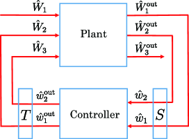
Figure 4: Coherent feedback control of the 3 input-output plant system via the 2 input-output controller.

where $S_{j}$ and $T_{j}$ are $2\times 2$ unitary matrices representing the scattering process of the fields; recall that the scattering process $\hat{A}^{\rm out}=e^{i\theta}\hat{A}$ with $\theta\in\mathbb{R}$ the phase shift can be represented in the quadrature form as

$$\left[\begin{array}[]{cc}\hat{Q}^{\rm out}\\ \hat{P}^{\rm out}\\ \end{array}\right]=S(\theta)\left[\begin{array}[]{cc}\hat{Q}\\ \hat{P}\\ \end{array}\right]=\left[\begin{array}[]{cc}\cos\theta&-\sin\theta\\ \sin\theta&\cos\theta\\ \end{array}\right]\left[\begin{array}[]{cc}\hat{Q}\\ \hat{P}\\ \end{array}\right].$$

Combining the above equations, we find that the whole closed-loop system with the augmented variable $\hat{x}_{{\scriptscriptstyle E}}=[\hat{x}^{\top},\hat{x}_{\scriptscriptstyle K}^{\top}]^{\top}$ is given by

$$\frac{d\hat{x}_{{\scriptscriptstyle E}}}{dt} =A_{{\scriptscriptstyle E}}\hat{x}_{{\scriptscriptstyle E}}+B_{{\scriptscriptstyle E}}\hat{W}_{1}+b_{{\scriptscriptstyle E}}\hat{f},$$

$$\hat{W}_{3}^{\rm out} =C_{{\scriptscriptstyle E}}\hat{x}_{{\scriptscriptstyle E}}+D_{{\scriptscriptstyle E}}\hat{W}_{1},$$ (40)

where

$$A_{{\scriptscriptstyle E}} =\left[\begin{array}[]{c}A+B\{T_{1}S_{1}+T_{2}S_{2}(T_{1}S_{1}+I_{2})\}C\\[4.30554pt] B_{\scriptscriptstyle K}\{(I_{2}+S_{2}T_{1})S_{1}+S_{2}\}C\end{array}\right.$$

$$~{}~{}~{}~{}~{}~{}~{}~{}~{}~{}~{}~{}~{}~{}~{}~{}~{}~{}~{}~{}~{}~{}~{}~{}~{}~{}~{}\left.\begin{array}[]{c}B\{T_{1}+T_{2}(I_{2}+S_{2}T_{1})\}C_{\scriptscriptstyle K}\\[4.30554pt] A_{\scriptscriptstyle K}+B_{\scriptscriptstyle K}S_{2}T_{1}C_{\scriptscriptstyle K}\end{array}\right].$$

$$B_{{\scriptscriptstyle E}} =\left[\begin{array}[]{c}B(I_{2}+T_{1}S_{1}+T_{2}S_{2}T_{1}S_{1})\\[4.30554pt] B_{{\scriptscriptstyle K}}(I_{2}+S_{2}T_{1})S_{1}\\ \end{array}\right]$$

$$C_{{\scriptscriptstyle E}} =\left[\begin{array}[]{cc}(T_{2}S_{2}T_{1}S_{1}+T_{2}S_{2}+I_{2})C{}&~{}T_{2}(S_{2}T_{1}+I_{2})C_{\scriptscriptstyle K}\\ \end{array}\right]$$

$$D_{{\scriptscriptstyle E}} =T_{2}S_{2}T_{1}S_{1},~{}~{}b_{{\scriptscriptstyle E}}=\left[\begin{array}[]{cc}b^{\top}&O\\ \end{array}\right]^{\top}.$$

Therefore, the desired system structure of the form (10) is realized if we take

$$S_{2}T_{1}=-I_{2}.$$ (41)

In addition, it is required that the back-action noise $\hat{Q}_{1}$ dose not appear directly in $\hat{P}_{3}^{\rm out}$, which can be realized by taking

$$D_{{\scriptscriptstyle E}}=-T_{2}S_{1}=\pm I_{2}.$$ (42)

Here we set $S_{j}$ and $T_{j}$ to be the $\pi/2$-phase shifter (see Fig. 5) to satisfy the above conditions (41) and (42);

$$S_{j}=T_{j}=S=\left[\begin{array}[]{cc}0&-1\\ 1&0\\ \end{array}\right]~{}~{}(j=1,2).$$ (45)

As a consequence, we end up with

$$A_{{\scriptscriptstyle E}}=\left[\begin{array}[]{cc}A-BC&BSC_{\scriptscriptstyle K}\\ B_{\scriptscriptstyle K}SC&A_{\scriptscriptstyle K}-B_{\scriptscriptstyle K}C_{\scriptscriptstyle K}\end{array}\right],~{}~{}B_{{\scriptscriptstyle E}}=\left[\begin{array}[]{c}B\\ O\\ \end{array}\right],$$ (50)

$$C_{{\scriptscriptstyle E}}=\left[\begin{array}[]{cc}C&O\\ \end{array}\right],~{}~{}D_{{\scriptscriptstyle E}}=I_{2},~{}~{}b_{{\scriptscriptstyle E}}=\left[\begin{array}[]{cc}b^{\top}&O\\ \end{array}\right]^{\top}.$$ (53)

This is certainly of the form (10) with $D_{\scriptscriptstyle K}=-I_{2}$. Hence, we can now directly apply the geometric control theory to design a coherent feedback controller achieving BAE; that is, our aim is to find $(A_{\scriptscriptstyle K},B_{\scriptscriptstyle K},C_{\scriptscriptstyle K})$ such that, for the closed-loop system (III.2), the back-action noise $\hat{Q}_{1}$ (the first element of $\hat{W}_{1}$) does not appear in the measurement output $\hat{P}_{3}^{\rm out}$ (the second element of $\hat{W}_{3}^{\rm out}$). Note that those matrices must satisfy the physical realizability condition (22), and thus they cannot be freely chosen. We need to take into account this additional constraint when applying the geometric control theory to determine the controller matrices.

III.3 Coherent feedback realization of BAE in the opto-mechanical system

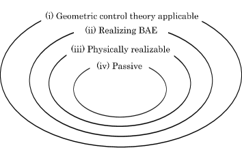
Figure 6: The set of controllers satisfying the condition in each step. For the controller to be a quantum system, it must be included in the set (iii). In the set (iv), all the controllers are equivalent up to the phase shift.

Here we apply the coherent feedback scheme elaborated in Section III.2 to the opto-mechanical system studied in Section II.3. The goal is, as mentioned before, to determine the controller matrices $(A_{\scriptscriptstyle K},B_{\scriptscriptstyle K},C_{\scriptscriptstyle K})$ such that the closed-loop system achieves BAE. Here, we provide a step-by-step procedure to solve this problem; the relationships of the class of controllers determined in each step is depicted in Fig. 6.

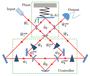
Figure 5: Coherent feedback controlled system composed of the opto-mechanical oscillator, for realizing BAE. The triangle represents the $\pi/2$-phase shifter corresponding to Eq. (45).

(i) First, to apply the geometric control theory developed above, we need to modify the plant system so that it is a 3 input-output linear quantum system; here we consider the plant composed of a mechanical oscillator and a 3-ports optical cavity, shown in Fig. 5. As assumed before, those ports have the same coupling constant $\kappa$. In this case the matrix $A$ given in Eq. (35) is replaced by

$$A=\left[\begin{array}[]{cccc}0&\omega_{\scriptscriptstyle m}&0&0\\ -\omega_{\scriptscriptstyle m}&0&g&0\\ 0&0&-3\kappa/2&0\\ g&0&0&-3\kappa/2\\ \end{array}\right].$$ (58)

Now we focus only on the back-action noise $\hat{Q}_{1}$ and the measurement output $\hat{P}_{3}^{\rm out}$; hence the closed-loop system (III.2) and (53), which ignores the shot noise term in the dynamical equation, is given by

$$\frac{d\hat{x}_{{\scriptscriptstyle E}}}{dt} =\left[\begin{array}[]{cc}A-BC&BSC_{\scriptscriptstyle K}\\ B_{\scriptscriptstyle K}SC&A_{\scriptscriptstyle K}-B_{\scriptscriptstyle K}C_{\scriptscriptstyle K}\end{array}\right]\hat{x}_{{\scriptscriptstyle E}}$$

$$~{}~{}~{}~{}~{}~{}~{}~{}~{}~{}~{}~{}~{}~{}~{}~{}~{}~{}~{}~{}~{}~{}~{}~{}~{}~{}~{}~{}~{}~{}+\left[\begin{array}[]{c}E\\ O\\ \end{array}\right]\hat{Q}_{1}+\left[\begin{array}[]{c}b\\ O\\ \end{array}\right]\hat{f},$$

$$\hat{P}_{3}^{\rm out} =\left[\begin{array}[]{cc}H&O\\ \end{array}\right]\hat{x}_{{\scriptscriptstyle E}}+\hat{P}_{1},$$

where $B=B_{1}$, $C=C_{1}$, and $b$ are given in Eq. (35), and

$$E=-\sqrt{\kappa}\left[\begin{array}[]{cccc}0&0&1&0\\ \end{array}\right]^{\top},~{}~{}~{}H=\sqrt{\kappa}\left[\begin{array}[]{cccc}0&0&0&1\\ \end{array}\right].$$

This system is certainly of the form (10), where now $D_{\scriptscriptstyle K}=-I_{2}$.

(ii) In the next step we apply Theorem 1 to check if there exists a feedback controller such that the above closed-loop system achieves BAE; recall that the necessary and sufficient condition is Eq. (18), i.e., $\mathcal{E}\subseteq\mathcal{V}_{1}\subseteq\mathcal{V}_{2}\subseteq\mathcal{H}$, where now

$$\mathcal{E} ={\rm Im}\hskip 1.9919ptE={\rm span}\left\{\left[\begin{array}[]{c}0\\ 0\\ 1\\ 0\\ \end{array}\right]\right\},$$

$$\mathcal{H} ={\rm Ker}\hskip 1.9919ptH={\rm span}\left\{\left[\begin{array}[]{c}1\\ 0\\ 0\\ 0\\ \end{array}\right],\left[\begin{array}[]{c}0\\ 1\\ 0\\ 0\\ \end{array}\right],\left[\begin{array}[]{c}0\\ 0\\ 1\\ 0\\ \end{array}\right]\right\}.$$

To check if this solvability condition is satisfied, we use Corollary 1; from $\mathcal{E}\cap\mathcal{C}={\rm Im}\hskip 1.9919ptE\cap{\rm Ker}\hskip 1.9919ptC=\phi$ and $\mathcal{H}\oplus\mathcal{B}={\rm Ker}\hskip 1.9919ptH\oplus{\rm Im}\hskip 1.9919ptB=\mathbb{R}^{4}$, the algorithms given in Appendix A yield

$$\mathcal{V}_{*}{\scriptscriptstyle(\mathcal{C},\mathcal{E})}=\mathcal{E},~{}~{}~{}\mathcal{V}^{*}{\scriptscriptstyle(\mathcal{B},\mathcal{H})}=\mathcal{H},$$ (59)

implying that the condition in Corollary 1, i.e., $\mathcal{V}_{*}{\scriptscriptstyle(\mathcal{C},\mathcal{E})}\subseteq\mathcal{V}^{*}{\scriptscriptstyle(\mathcal{B},\mathcal{H})}$, is satisfied. Thus, we now see that the BAE problem is solvable, as long as there is no constraint on the controller parameters.

Next we aim to determine the controller matrices $(A_{\scriptscriptstyle K},B_{\scriptscriptstyle K},C_{\scriptscriptstyle K})$, using Theorem 2. First we set $\mathcal{V}_{1}=\mathcal{V}_{*}{\scriptscriptstyle(\mathcal{C},\mathcal{E})}=\mathcal{E}$ and $\mathcal{V}_{2}=\mathcal{V}^{*}{\scriptscriptstyle(\mathcal{B},\mathcal{H})}=\mathcal{H}$; note that $(\mathcal{V}_{1},\mathcal{V}_{2})$ is a $(C,A,B)$-pair. Then, from Theorem 2, there exists a feedback controller with dimension ${\rm dim}\,\mathcal{X}_{\scriptscriptstyle K}={\rm dim}\,\mathcal{V}_{2}-{\rm dim}\,\mathcal{V}_{1}=2$. Moreover, noting again that $D_{\scriptscriptstyle K}=-I_{2}$, there exist matrices $F\in\mathcal{F}(\mathcal{V}_{2})$, $G\in\mathcal{G}(\mathcal{V}_{1})$, and $N$ such that

$${\rm Ker}\hskip 1.9919ptF_{0} ={\rm Ker}\hskip 1.9919pt(F+C)\supseteq\mathcal{V}_{1},$$

$${\rm Im}\hskip 1.9919ptG_{0} ={\rm Im}\hskip 1.9919pt(G+B)\subseteq\mathcal{V}_{2},~{}~{}{\rm Ker}\hskip 1.9919ptN=\mathcal{V}_{1}.$$

These conditions lead to

$$F =\left[\begin{array}[]{cccc}f_{\scriptscriptstyle 11}&f_{\scriptscriptstyle 12}&-\sqrt{\kappa}&f_{\scriptscriptstyle 14}\\ \frac{g}{\sqrt{\kappa}}&0&0&f_{\scriptscriptstyle 24}\\ \end{array}\right],~{}~{}G=\left[\begin{array}[]{cc}0&g_{\scriptscriptstyle 12}\\ -\frac{g}{\sqrt{\kappa}}&g_{\scriptscriptstyle 22}\\ g_{\scriptscriptstyle 31}&g_{\scriptscriptstyle 32}\\ 0&\sqrt{\kappa}\\ \end{array}\right],$$

$$N =\left[\begin{array}[]{cccc}n_{\scriptscriptstyle 11}&n_{\scriptscriptstyle 12}&0&n_{\scriptscriptstyle 14}\\ n_{\scriptscriptstyle 21}&n_{\scriptscriptstyle 22}&0&n_{\scriptscriptstyle 24}\\ \end{array}\right],$$

where $f_{ij},g_{ij}$, and $n_{ij}$ are free parameters. Then the controller matrices $(A_{\scriptscriptstyle K},B_{\scriptscriptstyle K},C_{\scriptscriptstyle K})$ can be identified by Eq. (II.1) with the above matrices $(F,G,N)$; specifically, by substituting $C_{\scriptscriptstyle K}\to SC_{\scriptscriptstyle K}$, $B_{\scriptscriptstyle K}\to B_{\scriptscriptstyle K}S$, and $A_{\scriptscriptstyle K}\to A_{\scriptscriptstyle K}-B_{\scriptscriptstyle K}C_{\scriptscriptstyle K}$ in Eq. (II.1), we have

$$SC_{\scriptscriptstyle K}N=F+C,$$

$$B_{\scriptscriptstyle K}S=-N(G+B),$$

$$(A_{\scriptscriptstyle K}-B_{\scriptscriptstyle K}C_{\scriptscriptstyle K})N=N(A+BF_{0}+GC),$$

which yield

$$A_{\scriptscriptstyle K}=N(A+BF_{0}+GC+G_{0}F_{0})N^{+},$$

$$B_{\scriptscriptstyle K}=-NG_{0}\Sigma,$$

$$C_{\scriptscriptstyle K}=\Sigma F_{0}N^{+},$$ (60)

where $N^{+}$ is the right inverse to $N$, i.e., $NN^{+}=I_{2}$.

(iii) Note again that the controller (III.2) has to satisfy the physical realizability condition (22), which is now $A_{\scriptscriptstyle K}\Sigma+\Sigma A_{\scriptscriptstyle K}^{\top}+2B_{\scriptscriptstyle K}\Sigma B_{\scriptscriptstyle K}^{\top}=O$ and $B_{\scriptscriptstyle K}=\Sigma C_{\scriptscriptstyle K}^{\top}\Sigma$. These constraints are represented in terms of the parameters as follows:

$$f_{\scriptscriptstyle 12}=-g_{\scriptscriptstyle 12},~{}~{}f_{\scriptscriptstyle 11}=g_{\scriptscriptstyle 22},~{}~{}n_{\scriptscriptstyle 11}n_{\scriptscriptstyle 22}-n_{\scriptscriptstyle 12}n_{\scriptscriptstyle 21}=-1,~{}$$

$$f_{\scriptscriptstyle 12}n_{\scriptscriptstyle 1}=f_{\scriptscriptstyle 11}n_{\scriptscriptstyle 2}-f_{\scriptscriptstyle 14},~{}~{}f_{\scriptscriptstyle 24}+\sqrt{\kappa}=\frac{g}{\sqrt{\kappa}}n_{\scriptscriptstyle 2},$$

$$\left(\frac{3}{2}\kappa+\sqrt{\kappa}f_{\scriptscriptstyle 24}\right)n_{\scriptscriptstyle 1}+\omega_{\scriptscriptstyle m}n_{\scriptscriptstyle 2}=-\sqrt{\kappa}f_{\scriptscriptstyle 11},$$

$$\omega_{\scriptscriptstyle m}n_{\scriptscriptstyle 1}-\left(\frac{3}{2}\kappa+\sqrt{\kappa}f_{\scriptscriptstyle 24}\right)n_{\scriptscriptstyle 2}=\sqrt{\kappa}f_{\scriptscriptstyle 12},$$ (61)

where $n_{\scriptscriptstyle 1}=n_{\scriptscriptstyle 11}n_{\scriptscriptstyle 24}-n_{\scriptscriptstyle 14}n_{\scriptscriptstyle 21}$ and $n_{\scriptscriptstyle 2}=n_{\scriptscriptstyle 12}n_{\scriptscriptstyle 24}-n_{\scriptscriptstyle 14}n_{\scriptscriptstyle 22}$. This is one of our main results; the linear controller (III.2) achieving BAE for the opto-mechanical oscillator can be fully parametrized by Eq. (III.3) satisfying the condition (III.3). We emphasize that this full parametrization of the controller can be obtained thanks to the general problem formulation based on the geometric control theory.

(iv) In practice, of course, we need to determine a concrete set of parameters to construct the controller. Especially here let us consider a passive system; this is a static quantum system such as an empty optical cavity. The main reason for choosing a passive system rather than a non-passive (or active) one such as an optical parametric oscillator is that, due to the external pumping energy, the latter could become fragile and also its physical implementation must be more involved compared to a passive system Walls2008 . Now the condition for the system $(A_{\scriptscriptstyle K},\,B_{\scriptscriptstyle K},\,C_{\scriptscriptstyle K})$ to be passive is given by $\Sigma A_{\scriptscriptstyle K}\Sigma=-A_{\scriptscriptstyle K}$ and $\Sigma B_{\scriptscriptstyle K}\Sigma=-B_{\scriptscriptstyle K}$; the general result of this fact is given in Theorem 3 in Appendix B. From these conditions, the system parameters are imposed to satisfy, in addition to Eq. (III.3), the following equalities:

$$f_{\scriptscriptstyle 12}=\frac{g}{\sqrt{\kappa}},~{}~{}f_{\scriptscriptstyle 11}=0,~{}~{}n_{\scriptscriptstyle 11}=-n_{\scriptscriptstyle 22},~{}~{}n_{\scriptscriptstyle 12}=n_{\scriptscriptstyle 21}.$$ (62)

There is still some freedom in determining $n_{ij}$, which however corresponds to simply the phase shift at the input-output ports of the controller, as indicated from Eq. (III.3). Thus, the passive controller achieving BAE in this example is unique up to the phase shift. Here particularly we chose $n_{\scriptscriptstyle 11}=1$ and $n_{\scriptscriptstyle 12}=0$. Then the controller matrices (III.3) satisfying Eqs. (III.3) and (62) are determined as

$$A_{\scriptscriptstyle K}=\left[\begin{array}[]{cc}-\frac{~{}g^{2}}{\kappa}&-\omega_{\scriptscriptstyle m}\\ \omega_{\scriptscriptstyle m}&-\frac{~{}g^{2}}{\kappa}\\ \end{array}\right],~{}~{}C_{\scriptscriptstyle K}=-B_{\scriptscriptstyle K}^{\top}=\left[\begin{array}[]{cc}\frac{g}{\sqrt{\kappa}}&0\\ 0&\frac{g}{\sqrt{\kappa}}\\ \end{array}\right].$$

As illustrated in Fig. 5, the controller specified by these matrices can be realized as a single-mode, 2-inputs and 2-outputs optical cavity with decay rate $g^{2}/\kappa$ and detuning $-\omega_{\scriptscriptstyle m}$. In other words, if we take the cavity with the following Hamiltonian and the coupling operator ($\hat{a}_{3}=(\hat{q}_{3}+i\hat{p}_{3})/\sqrt{2}$ is the cavity mode)

$$\hat{H}_{\scriptscriptstyle K} =\Delta\hat{a}^{\ast}_{3}\hat{a}_{3}=\frac{\Delta}{2}(\hat{q}_{3}^{2}+\hat{p}_{3}^{2}),$$

$$\hat{L}_{\scriptscriptstyle K} =\sqrt{\kappa_{\scriptscriptstyle K}}\hat{a}_{3}=\sqrt{\frac{\kappa_{\scriptscriptstyle K}}{2}}(\hat{q}_{3}+i\hat{p}_{3}),$$ (63)

then to satisfy the BAE condition the controller parameters $(\Delta,\kappa_{\scriptscriptstyle K})$ must satisfy

$$\Delta=-\omega_{\scriptscriptstyle m},~{}~{}~{}\kappa_{\scriptscriptstyle K}=g^{2}/\kappa.$$ (64)

Summarizing, the above-designed sensing system composed of the opto-mechanical oscillator (plant) and the optical cavity (controller), which are combined via coherent feedback, satisfies the BAE condition. Hence, it can work as a high-precision detector of the force $\hat{f}$ below the SQL, particularly when the $\hat{P}_{1}$-squeezed probe input field is used; this fact will be demonstrated in Section V.

IV Direct interaction scheme

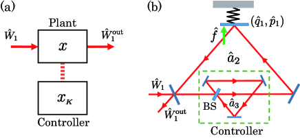
Figure 7: (a) General configuration of direct interaction scheme. (b) Physical implementation of the passive direct interaction controller for the opto-mechanical oscillator.

In this section, we study another control scheme for achieving BAE. As illustrated in Fig. 7 (a), the controller in this case is directly connected to the plant, not through a coherent feedback; hence this scheme is called the direct interaction. The controller is characterized by the following two Hamiltonians:

$$\hat{H}_{\scriptscriptstyle K}=\frac{1}{2}\hat{x}_{\scriptscriptstyle K}^{\top}R_{\scriptscriptstyle K}\hat{x}_{\scriptscriptstyle K},~{}\hat{H}_{\rm int}=\frac{1}{2}(\hat{x}^{\top}R_{1}\hat{x}_{\scriptscriptstyle K}+\hat{x}_{\scriptscriptstyle K}^{\top}R_{2}\hat{x}),$$ (65)

where $\hat{x}_{\scriptscriptstyle K}=[\hat{q}^{\scriptscriptstyle\prime}_{1},\hat{p}^{\scriptscriptstyle\prime}_{1},\ldots,\hat{q}^{\scriptscriptstyle\prime}_{n_{\scriptscriptstyle k}},\hat{p}^{\scriptscriptstyle\prime}_{n_{\scriptscriptstyle k}}]^{\top}$ is the vector of controller variables with $n_{\scriptscriptstyle k}$ the number of modes of the controller. $\hat{H}_{\scriptscriptstyle K}$ is the controller’s self Hamiltonian with $R_{\scriptscriptstyle K}\in\mathbb{R}^{2n_{\scriptscriptstyle k}\times 2n_{\scriptscriptstyle k}}$. Also $\hat{H}_{\rm int}$ with $R_{1}\in\mathbb{R}^{2n\times 2n_{\scriptscriptstyle k}}$, $R_{2}\in\mathbb{R}^{2n_{\scriptscriptstyle k}\times 2n}$ represents the coupling between the plant and the controller. Note that, for the Hamiltonians $\hat{H}_{\scriptscriptstyle K}$ and $\hat{H}_{\rm int}$ to be Hermitian, the matrices must satisfy $R_{\scriptscriptstyle K}=R_{\scriptscriptstyle K}^{\top}$ and $R_{1}^{\top}=R_{2}$; these are the physical realizability conditions in the scenario of direct interaction. In particular, here we consider a plant system interacting with a single probe field $\hat{W}_{1}$, with coupling matrices $B_{1}=B$ and $C_{1}=C$. Then, the whole dynamics of the augmented system with variable $\hat{x}_{{\scriptscriptstyle E}}=[\hat{x}^{\top},\hat{x}_{\scriptscriptstyle K}^{\top}]^{\top}$ is given by

$$\frac{d\hat{x}_{{\scriptscriptstyle E}}}{dt} =A_{{\scriptscriptstyle E}}\hat{x}_{{\scriptscriptstyle E}}+B_{{\scriptscriptstyle E}}\hat{W}_{1}+b_{{\scriptscriptstyle E}}\hat{f},$$

$$\hat{W}_{1}^{\rm out} =C_{{\scriptscriptstyle E}}\hat{x}_{{\scriptscriptstyle E}}+\hat{W}_{1},$$ (66)

where

$$A_{{\scriptscriptstyle E}} =\left[\begin{array}[]{cc}~{}A{}{}&\Sigma_{n}R_{1}{}{}\\ \Sigma_{n_{\scriptscriptstyle k}}R_{2}&\Sigma_{n_{\scriptscriptstyle k}}R_{\scriptscriptstyle K}\\ \end{array}\right],~{}~{}B_{{\scriptscriptstyle E}}=\left[\begin{array}[]{c}B\\ O\\ \end{array}\right],$$ (71)

$$C_{{\scriptscriptstyle E}} =\left[\begin{array}[]{cc}C&O\\ \end{array}\right],~{}~{}b_{{\scriptscriptstyle E}}=\left[\begin{array}[]{cc}b^{\top}&O\\ \end{array}\right]^{\top}.$$ (74)

Note that $B_{{\scriptscriptstyle E}}$, $C_{{\scriptscriptstyle E}}$, and $b_{{\scriptscriptstyle E}}$ are the same matrices as those in Eq. (53). Also, comparing the matrices (17) and (71), we have that $D_{\scriptscriptstyle K}=O$, which thus leads to $F=F_{0}$ and $G=G_{0}$ in Theorem 2. Now, again for the opto-mechanical system illustrated in Fig. 2, let us aim to design the direct interaction controller, so that the whole system (IV) achieves BAE; that is, the problem is to determine the matrices $(R_{\scriptscriptstyle K},R_{1},R_{2})$ so that the back-action noise $\hat{Q}_{1}$ does not appear in the measurement output $\hat{P}_{1}^{\rm out}$. For this purpose, we go through the same procedure as that taken in Section III.3.

(i) Because of the structure of the matrices $B_{{\scriptscriptstyle E}}$ and $C_{{\scriptscriptstyle E}}$, the system is already of the form (10), where the geometric control theory is directly applicable.

(ii) Because we now focus on the same plant system as that in Section III.3, the same conclusion is obtained; that is, the BAE problem is solvable as long as there is no constraint on the controller matrices $(R_{\scriptscriptstyle K},R_{1},R_{2})$.

The controller matrices can be determined in a similar way to Section III.3 as follows. First, because the $(C,A,B)$-pair $(\mathcal{V}_{1},\mathcal{V}_{2})$ is the same as before, it follows that ${\rm dim}\,\mathcal{X}_{{\scriptscriptstyle K}}=2$, i.e., $n_{\scriptscriptstyle k}=1$. Then, from Theorem 2 with the fact that $F=F_{0}$ and $G=G_{0}$, we find that the direct interaction controller can be parameterized as follows:

$$R_{\scriptscriptstyle K}=-\Sigma N(A+BF+GC)N^{+},$$

$$R_{1}=-\Sigma_{2}BFN^{+},$$

$$R_{2}=\Sigma NGC,$$ (75)

The matrices $F$, $G$, and $N$ satisfy ${\rm Ker}\hskip 1.9919ptF\supseteq\mathcal{V}_{1},{\rm Im}\hskip 1.9919ptG\subseteq\mathcal{V}_{2}$, and ${\rm Ker}\hskip 1.9919ptN=\mathcal{V}_{1}$, which lead to

$$F =\left[\begin{array}[]{cccc}f_{\scriptscriptstyle 11}&f_{\scriptscriptstyle 12}&0&f_{\scriptscriptstyle 14}\\ \frac{g}{\sqrt{\kappa}}&0&0&f_{\scriptscriptstyle 24}\\ \end{array}\right],~{}~{}G=\left[\begin{array}[]{cc}0&g_{\scriptscriptstyle 12}\\ -\frac{g}{\sqrt{\kappa}}&g_{\scriptscriptstyle 22}\\ g_{\scriptscriptstyle 31}&g_{\scriptscriptstyle 32}\\ 0&0\\ \end{array}\right],$$ (82)

$$N =\left[\begin{array}[]{cccc}n_{\scriptscriptstyle 11}&n_{\scriptscriptstyle 12}&0&n_{\scriptscriptstyle 14}\\ n_{\scriptscriptstyle 21}&n_{\scriptscriptstyle 22}&0&n_{\scriptscriptstyle 24}\\ \end{array}\right],$$ (85)

where $f_{ij},g_{ij}$, and $n_{ij}$ are free parameters.

(iii) The controller matrices have to satisfy the physical realizability conditions $R_{\scriptscriptstyle K}=R_{\scriptscriptstyle K}^{\top}$ and $R_{1}^{\top}=R_{2}$; these constraints impose the parameters to satisfy

$$f_{\scriptscriptstyle 12}=-g_{\scriptscriptstyle 12},~{}~{}f_{\scriptscriptstyle 11}=g_{\scriptscriptstyle 22},~{}~{}n_{\scriptscriptstyle 11}n_{\scriptscriptstyle 22}-n_{\scriptscriptstyle 12}n_{\scriptscriptstyle 21}=-1,$$

$$f_{\scriptscriptstyle 12}n_{\scriptscriptstyle 1}=f_{\scriptscriptstyle 11}n_{\scriptscriptstyle 2}-f_{\scriptscriptstyle 14},~{}~{}f_{\scriptscriptstyle 24}=\frac{g}{\sqrt{\kappa}}n_{\scriptscriptstyle 2},$$

$$\left(\frac{\kappa}{2}+\sqrt{\kappa}f_{\scriptscriptstyle 24}\right)n_{\scriptscriptstyle 1}+\omega_{\scriptscriptstyle m}n_{\scriptscriptstyle 2}=-\sqrt{\kappa}f_{\scriptscriptstyle 11},~{}~{}$$

$$\omega_{\scriptscriptstyle m}n_{\scriptscriptstyle 1}-\left(\frac{\kappa}{2}+\sqrt{\kappa}f_{\scriptscriptstyle 24}\right)n_{\scriptscriptstyle 2}=\sqrt{\kappa}f_{\scriptscriptstyle 12},$$ (86)

where $n_{\scriptscriptstyle 1}=n_{\scriptscriptstyle 11}n_{\scriptscriptstyle 24}-n_{\scriptscriptstyle 14}n_{\scriptscriptstyle 21}$ and $n_{\scriptscriptstyle 2}=n_{\scriptscriptstyle 12}n_{\scriptscriptstyle 24}-n_{\scriptscriptstyle 14}n_{\scriptscriptstyle 22}$.
Equations (IV), (82), and (IV) provide the full parametrization of the direct interaction controller.

(iv) To specify a set of parameters, as in the case of Section III.3, let us aim to design a passive controller. From Theorem 4 in Appendix B, $R_{\scriptscriptstyle K}$ and $R_{2}=R_{1}^{\top}$ satisfy the condition $\Sigma R_{\scriptscriptstyle K}\Sigma=-R_{\scriptscriptstyle K}$ and $\Sigma R_{2}\Sigma_{2}=-R_{2}$, which lead to the same equalities given in Eq. (62). Then, setting the parameters to be $n_{\scriptscriptstyle 11}=1$ and $n_{\scriptscriptstyle 12}=0$, we can determine the matrices $R_{\scriptscriptstyle K}$ and $R_{2}$ as follows:

$$R_{\scriptscriptstyle K}=\left[\begin{array}[]{cc}-\omega_{\scriptscriptstyle m}&0\\ 0&-\omega_{\scriptscriptstyle m}\\ \end{array}\right],~{}~{}R_{2}=R_{1}^{\top}=\left[\begin{array}[]{cccc}0&0&g&0\\ 0&0&0&g\\ \end{array}\right].$$

The controller specified by these matrices can be physically implemented as illustrated in Fig. 7 (b); that is, it is a single-mode detuned cavity with Hamiltonian $\hat{H}_{\scriptscriptstyle K}=-\omega_{\scriptscriptstyle m}\hat{a}^{\ast}_{3}\hat{a}_{3}$, which couples to the plant through a beam-splitter (BS) represented by $\hat{H}_{\rm int}=g(\hat{a}_{3}\hat{a}^{*}_{2}+\hat{a}^{*}_{3}\hat{a}_{2})$.

Remark: We can employ an active controller, as proposed in Tsang2010 . In this case the interaction Hamiltonian is given by $\hat{H}_{\rm int}=g_{\scriptscriptstyle\rm B}(\hat{a}_{3}\hat{a}^{*}_{2}+\hat{a}^{*}_{3}\hat{a}_{2})+g_{\scriptscriptstyle\rm D}(\hat{a}_{3}\hat{a}_{2}+\hat{a}^{*}_{3}\hat{a}^{*}_{2})$, while the system’s self-Hamiltonian is the same as above; $\hat{H}_{\scriptscriptstyle K}=-\omega_{\scriptscriptstyle m}\hat{a}^{\ast}_{3}\hat{a}_{3}$. That is, the controller couples to the plant through a non-degenerate optical parametric amplification process in addition to the BS interaction. To satisfy the BAE condition, the parameters must satisfy $g_{\scriptscriptstyle\rm B}+g_{\scriptscriptstyle\rm D}=g$. Note that this direct interaction controller can be specified, in the full-parameterization (IV), (82), and (IV), by

$$f_{\scriptscriptstyle 11}=f_{\scriptscriptstyle 12}=f_{\scriptscriptstyle 14}=0,~{}~{}n_{\scriptscriptstyle 11}=-n_{\scriptscriptstyle 22}=1,~{}~{}n_{\scriptscriptstyle 12}=n_{\scriptscriptstyle 21}=0.$$

V Approximate Back-Action Evasion

We have demonstrated in Sections III.3 and IV that the BAE condition can be achieved by engineering an appropriate auxiliary system and connecting it to the plant. However, in a practical situation, it cannot be expected to realize such perfect BAE due to several experimental imperfections. Hence, in a realistic setup, we should modify our strategy for engineering a sensor so that it would accomplish approximate BAE. Then, looking back into Section II.3 where the BAE condition, $\Xi_{Q}(s)=0~{}\forall s$, was obtained, we are naturally led to consider the following optimization problem to design an auxiliary system achieving the approximate BAE:

$$\min\Big{\|}\frac{\Xi_{Q}(s)}{\Xi_{f}(s)}\Big{\|},$$ (87)

where $\|\bullet\|$ denotes a valid norm of a complex function. In particular, in the field of robust control theory, the following $H_{2}$ norm and the $H_{\infty}$ norm are often used Zhou1996 :

$$\|\Xi\|_{2}=\sqrt{\frac{1}{2\pi}\int_{-\infty}^{\infty}|\Xi(i\omega)|^{2}d\omega},~{}~{}~{}\|\Xi\|_{\infty}=\max_{\omega}|\Xi(i\omega)|.$$

That is, the $H_{2}$ or $H_{\infty}$ control theory provides a general procedure for synthesizing a feedback controller that minimizes the above norm. In this paper, we take the $H_{2}$ norm, mainly owing to the broadband noise-reduction nature of the $H_{2}$ controller. Then, rather than pursuing an optimal quantum $H_{2}$ controller based on the quantum $H_{2}$ control theory NurdinLQG2009 ; Hamerly2012 , here we take the following geometric-control-theoretical approach to solve the problem (87). That is, first we apply the method developed in Section III or IV to the idealized system and obtain the controller achieving BAE; then, in the practical setup containing some unwanted noise, we make a local modification of the controller parameters obtained in the first step, to minimize the cost $\|\Xi_{Q}(s)/\Xi_{f}(s)\|_{2}$.

As a demonstration, here we consider the coherent feedback control for the opto-mechanical system studied in Section II.3, which is now subjected to the thermal noise $\hat{f}_{\rm th}$. Following the above-described policy, we employ the coherent feedback controller constructed for the idealized system that ignores $\hat{f}_{\rm th}$, leading to the controller given by Eqs. (63) and (64), illustrated in Fig. 5. The closed-loop system with variable $\hat{x}_{{\scriptscriptstyle E}}=[\hat{x}^{\top},\hat{x}_{\scriptscriptstyle K}^{\top}]^{\top}$, which now takes into account the realistic imperfections, then obeys the following dynamics:

$$\frac{d\hat{x}_{{\scriptscriptstyle E}}}{dt} =\widetilde{A}_{{\scriptscriptstyle E}}\hat{x}_{{\scriptscriptstyle E}}+B_{{\scriptscriptstyle E}}\hat{W}_{1}+b_{{\scriptscriptstyle E}}(\hat{f}_{\rm th}+\hat{f}),$$

$$\hat{W}_{3}^{\rm out} =C_{{\scriptscriptstyle E}}\hat{x}_{{\scriptscriptstyle E}}+\hat{W}_{1},$$ (88)

where

$$\widetilde{A}_{{\scriptscriptstyle E}}=\left[\begin{array}[]{cccc|cc}0&\omega_{\scriptscriptstyle m}&0&0&0&0\\ -\omega_{\scriptscriptstyle m}&-\gamma&g&0&0&0\\ 0&0&-\kappa/2&0&0&\sqrt{\kappa\kappa_{\scriptscriptstyle K}}\\ g&0&0&-\kappa/2&-\sqrt{\kappa\kappa_{\scriptscriptstyle K}}&0\\ \hline\cr 0&0&0&\sqrt{\kappa\kappa_{\scriptscriptstyle K}}&0&\Delta\\ 0&0&-\sqrt{\kappa\kappa_{\scriptscriptstyle K}}&0&-\Delta&0\\ \end{array}\right].$$

$B_{{\scriptscriptstyle E}}$, $C_{{\scriptscriptstyle E}}$, and $b_{{\scriptscriptstyle E}}$ are the same matrices given in Eq. (53). $\hat{f}_{\rm th}$ is the thermal noise satisfying $\langle\hat{f}_{\rm th}(t)\hat{f}_{\rm th}(t^{\prime})\rangle\simeq\bar{n}\delta(t-t^{\prime})$, where $\bar{n}$ is the mean phonon number at thermal equilibrium Giovannetti2001 ; Wimmer2014 . Note that the damping effect appears in the $(2,2)$ component of $\widetilde{A}_{{\scriptscriptstyle E}}$ due to the stochastic nature of $\hat{f}_{\rm th}$. Also, again, $\kappa_{\scriptscriptstyle K}$ and $\Delta$ are the decay rate and the detuning of the controller cavity, respectively. In the idealized setting where $\hat{f}_{\rm th}$ is negligible, the perfect BAE is achieved by choosing the parameters satisfying Eq. (64). The measurement output of this closed-loop system is, in the Laplace domain, represented by

$$\hat{P}_{3}^{\rm out}(s)=\widetilde{\Xi}_{f}(\hat{f}_{\rm th}(s)+\hat{f}(s))+\widetilde{\Xi}_{Q}\hat{Q}_{1}(s)+\widetilde{\Xi}_{P}\hat{P}_{1}(s).$$

The normalized noise power spectral density of $y_{3}(s)=\hat{P}_{3}^{\rm out}(s)/\widetilde{\Xi}_{f}(s)$ is calculated as

$$\widetilde{S}(\omega) =\langle|y_{3}(i\omega)-\hat{f}(i\omega)|^{2}\rangle$$

$$=\langle|\hat{f}_{\rm th}|^{2}\rangle+\left|\frac{\widetilde{\Xi}_{Q}}{\widetilde{\Xi}_{f}}\right|^{2}\langle|\hat{Q}_{1}|^{2}\rangle+\left|\frac{\widetilde{\Xi}_{P}}{\widetilde{\Xi}_{f}}\right|^{2}\langle|\hat{P}_{1}|^{2}\rangle.$$ (89)

The coefficient of the back-action noise is given by

$$\frac{\widetilde{\Xi}_{Q}(s)}{\widetilde{\Xi}_{f}(s)}=-\frac{\sqrt{\kappa}\{\kappa\kappa_{\scriptscriptstyle K}\Delta(s^{2}+\gamma s+\omega_{\scriptscriptstyle m}^{2})+g^{2}\omega_{\scriptscriptstyle m}(s^{2}+\Delta^{2})\}}{g\omega_{\scriptscriptstyle m}\sqrt{\gamma}\{(s+\kappa/2)(s^{2}+\Delta^{2})+\kappa\kappa_{\scriptscriptstyle K}s\}}.$$ (90)

Our goal is to find the optimal parameters $(\kappa_{\scriptscriptstyle K},\Delta)$ that minimize the $H_{2}$ norm of the transfer function, $\widetilde{\Xi}_{Q}/\widetilde{\Xi}_{f}$.

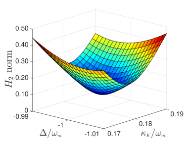
Figure 8: $H_{2}$ norm $\|\widetilde{\Xi}_{Q}/\widetilde{\Xi}_{f}\|_{2}$ versus the coupling constant $\kappa_{\scriptscriptstyle K}$ and the detuning $\Delta$.

The system parameters are taken as follows Wimmer2014 : $\omega_{\scriptscriptstyle m}/2\pi=0.5$ MHz, $\kappa/2\pi=1.0$ MHz, $\gamma/2\pi=5.0$ kHz, $g/2\pi=0.3$ MHz, $\bar{n}\simeq 8.33\times 10^{2}$, and the effective mass is $1.0\times 10^{-12}$ kg. We then have Fig. 8, showing $\|\widetilde{\Xi}_{Q}/\widetilde{\Xi}_{f}\|_{2}$ as a function of $\kappa_{\scriptscriptstyle K}$ and $\Delta$. This figure shows that there exists a unique pair of $(\kappa_{\scriptscriptstyle K}^{\rm opt},\Delta^{\rm opt})$ that minimizes the norm, and they are given by $\kappa_{\scriptscriptstyle K}^{\rm opt}/2\pi=0.093$ MHz and $\Delta^{\rm opt}/2\pi=-0.5$ MHz, which are actually close to the ideal values (64). Fig. 9 shows the value of Eq. (89) with these optimal parameters $(\kappa_{\scriptscriptstyle K}^{\rm opt},\Delta^{\rm opt})$, where the noise floor $\langle|\hat{f}_{\rm th}|^{2}\rangle$ is subtracted. The solid black line represents the SQL, which is now given by

$$\widetilde{S}_{\scriptscriptstyle\rm SQL}(\omega)=\frac{|(\omega^{2}-\omega_{\scriptscriptstyle m}^{2})-i\gamma\omega|}{\gamma\omega_{\scriptscriptstyle m}}.$$ (91)

Then the dot-dashed blue and dotted green lines indicate that, in the low frequency range, the coherent feedback controller can suppress the noise below the SQL, while, by definition, the noise power of the autonomous (i.e., uncontrolled) plant system is above the SQL. Moreover, this effect can be enhanced by injecting a $\hat{P}_{1}$-squeezed probe field (meaning $\langle|\hat{Q}_{1}|^{2}\rangle=e^{r}/2$ and $\langle|\hat{P}_{1}|^{2}\rangle=e^{-r}/2$) into the system. In fact the dashed red line in the figure illustrates the case $r=2$ (about 9 dB squeezing), showing the significant reduction of the noise power.

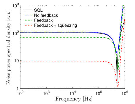
Figure 9: Normalized power spectral densities of the noise. The black solid line represents the SQL (91), and the dot-dashed blue line does the case without feedback. The dotted green and dashed red lines show the cases for the feedback controlled system, with coherent and squeezed probe field, respectively.

VI Conclusion

The main contribution of this paper is in that it first provides the general theory for constructing a back-action evading sensor for linear quantum systems, based on the well-developed classical geometric control theory. The power of the theory has been demonstrated by showing that, for the typical opto-mechanical oscillator, a full parametrization of the auxiliary coherent-feedback and direct interaction controller achieving BAE was derived, which contains the result of Tsang2010 . Note that, although we have studied a simple example for the purpose of demonstration, the real advantage of the theory developed in this paper will appear when dealing with more complicated multi-mode systems such as an opto-mechanical system containing a membrane Plenio2008 ; Meystre2008 ; Nakamura2016 ; Nielsen2016 . Another contribution of this paper is to provide a general procedure for designing an approximate BAE sensor under realistic imperfections; that is, an optimal approximate BAE system can be obtained by solving the minimization problem of the transfer function from the back-action noise to the measurement output. While in Section V we have provided a simple approach based on the geometric control theory for solving this problem, the $H_{2}$ or $H_{\infty}$ control theory could be employed for systematic design of an approximate BAE controller even for the above-mentioned complicated system. This is also an important future research direction of this work.

Appendix A: Algorithms for computing $\mathcal{V}^{*}$ and $\mathcal{V}_{*}$

The set of $(A,B)$-invariant subspaces has a unique maximum element contained in a given subspace $\mathcal{H}\subseteq\mathcal{X}$. This space, denoted by $\mathcal{V}^{*}{\scriptscriptstyle(\mathcal{B},\mathcal{H})}$, can be computed by the following algorithm:

$$\mathcal{V}^{*}~{} \mathchar 45\relax~{}{\bf algorithm:}~{}$$

$${\rm(Step~{}1)}~{}\mathcal{V}_{0}:=\mathcal{H},$$

$${\rm(Step~{}2)}~{}\mathcal{V}_{i}:=\mathcal{H}\cap A^{-1}(\mathcal{V}_{i-1}\oplus\mathcal{B})~{}~{}(i=1,2,\ldots),$$

$${\rm(Step~{}3)}~{}\mathcal{V}^{*}{\scriptscriptstyle(\mathcal{B},\mathcal{H})}=\mathcal{V}_{i}~{}~{}{\rm(if}~{}\mathcal{V}_{i}=\mathcal{V}_{i-1}~{}{\rm in~{}Step~{}2)}.$$

Similarly, the set of $(C,A)$-invariant subspaces has a unique minimum element containing a given subspace $\mathcal{E}\subseteq\mathcal{X}$, and this space, denoted by $\mathcal{V}_{*}{\scriptscriptstyle(\mathcal{C},\mathcal{E})}$, can be computed by the following algorithm:

$$\mathcal{V}_{*}~{} \mathchar 45\relax~{}{\bf algorithm:}~{}$$

$${\rm(Step~{}1)}~{}\mathcal{V}_{0}:=\mathcal{E},$$

$${\rm(Step~{}2)}~{}\mathcal{V}_{i}:=\mathcal{E}\oplus A(\mathcal{V}_{i-1}\cap\mathcal{C})~{}~{}(i=1,2,\ldots),$$

$${\rm(Step~{}3)}~{}\mathcal{V}_{*}{\scriptscriptstyle(\mathcal{C},\mathcal{E})}=\mathcal{V}_{i}~{}~{}{\rm(if}~{}\mathcal{V}_{i}=\mathcal{V}_{i-1}~{}{\rm in~{}Step~{}2)}.$$

Appendix B : Passivity condition of linear quantum systems

This appendix provides the passivity condition of a general linear quantum system. First note that the system dynamics (20) and (21), which can be represented as

$$\frac{d\hat{x}}{dt}=A\hat{x}+B\hat{W},~{}~{}~{}\hat{W}^{\rm out}=C\hat{x}+D\hat{W},$$ (92)

with $\hat{W}=[\hat{W}_{1},\ldots,\hat{W}_{m}]^{\top}$, has the following equivalent expression:

$$\frac{d}{dt}\left[\begin{array}[]{c}\hat{a}\\ \hat{a}^{\sharp}\\ \end{array}\right] =\mathscr{A}\left[\begin{array}[]{c}\hat{a}\\ \hat{a}^{\sharp}\\ \end{array}\right]+\mathscr{B}\left[\begin{array}[]{c}\hat{A}\\ \hat{A}^{\sharp}\\ \end{array}\right],$$ (99)

$$\left[\begin{array}[]{c}\hat{A}^{\rm out}\\ \hat{A}^{\rm out}\mbox{}^{\sharp}\\ \end{array}\right] =\mathscr{C}\left[\begin{array}[]{c}\hat{a}\\ \hat{a}^{\sharp}\\ \end{array}\right]+\mathscr{D}\left[\begin{array}[]{c}\hat{A}\\ \hat{A}^{\sharp}\\ \end{array}\right],$$ (106)

where $\hat{a}=[\hat{a}_{1},\ldots,\hat{a}_{n}]^{\top}$ and $\hat{A}=[\hat{A}_{1},\ldots,\hat{A}_{m}]^{\top}$ are vectors of annihilation operators. By definition, $\hat{a}^{\sharp}=[\hat{a}_{1}^{*},\ldots,\hat{a}_{n}^{*}]^{\top}$. The coefficient matrices are of the form

$$\mathscr{A} =\left[\begin{array}[]{cc}\mathscr{A}_{-}&\mathscr{A}_{+}\\ \mathscr{A}_{+}^{\sharp}&\mathscr{A}_{-}^{\sharp}\\ \end{array}\right],~{}~{}~{}\mathscr{B}=\left[\begin{array}[]{cc}\mathscr{B}_{-}&\mathscr{B}_{+}\\ \mathscr{B}_{+}^{\sharp}&\mathscr{B}_{-}^{\sharp}\\ \end{array}\right],$$ (111)

$$\mathscr{C} =\left[\begin{array}[]{cc}\mathscr{C}_{-}&~{}\mathscr{C}_{+}\\ \mathscr{C}_{+}^{\sharp}&~{}\mathscr{C}_{-}^{\sharp}\\ \end{array}\right],~{}~{}~{}\mathscr{D}=\left[\begin{array}[]{cc}\mathscr{D}_{-}&~{}\mathscr{D}_{+}\\ \mathscr{D}_{+}^{\sharp}&~{}\mathscr{D}_{-}^{\sharp}\\ \end{array}\right].$$ (116)

As in the case of (92), these matrices have to satisfy the physical realizability condition; see GoughPRA2010 ; PetersenMTNS2010 . The passivity condition of this system is defined as follows:

Definition 5:  The system (106) is said to be passive if the matrices satisfy $\mathscr{A}_{+}=O$ and $\mathscr{B}_{+}=O$, in addition to the physical realizability condition.

Note that a passive system is constituted only with annihilation operator variables; a typical optical realization of the passive system is an empty optical cavity. Moreover, $\mathscr{D}_{+}=O$ is already satisfied and $\mathscr{B}_{+}=O$ leads to $\mathscr{C}_{+}=O$. This is the reason why it is sufficient to consider the constraints only on $\mathscr{A}_{+}$ and $\mathscr{B}_{+}$. Then the goal here is to represent the conditions $\mathscr{A}_{+}=\mathscr{B}_{+}=O$ in terms of the coefficient matrices of Eq. (92). For this purpose, let us introduce the permutation matrix $P_{n}$ as follows; for a column vector $z=[z_{1},z_{2},\ldots,z_{2n}]^{\top}$, $P_{n}$ is defined through $P_{n}z=[z_{1},z_{3},\ldots,z_{2n-1},z_{2},z_{4},\ldots,z_{2n}]^{\top}$. Note that $P_{n}$ satisfies $P_{n}P_{n}^{\top}=P_{n}^{\top}P_{n}=I_{2n}$. Then, the coefficient matrices of the above two system representations are connected by

$$A =P_{n}^{\top}\tilde{\mathscr{A}}P_{n},~{}~{}B=P_{n}^{\top}\tilde{\mathscr{B}}P_{m},$$

$$C =P_{m}^{\top}\tilde{\mathscr{C}}P_{n},~{}~{}D=P_{m}^{\top}\tilde{\mathscr{D}}P_{m},$$

where

$$\tilde{\mathscr{A}}=\frac{1}{2}\left[\begin{array}[]{c}\mathscr{A}_{-}+\mathscr{A}_{-}^{\sharp}+\mathscr{A}_{+}+\mathscr{A}_{+}^{\sharp}{}{}{}{}{}{}{}\\ -i(\mathscr{A}_{-}-\mathscr{A}_{-}^{\sharp}+\mathscr{A}_{+}-\mathscr{A}_{+}^{\sharp}){}{}{}{}{}{}{}\end{array}\right.$$

$$\left.\begin{array}[]{c}~{}~{}~{}~{}~{}~{}~{}i(\mathscr{A}_{-}-\mathscr{A}_{-}^{\sharp}-\mathscr{A}_{+}+\mathscr{A}_{+}^{\sharp})\\ ~{}~{}~{}~{}~{}~{}~{}\mathscr{A}_{-}+\mathscr{A}_{-}^{\sharp}-(\mathscr{A}_{+}+\mathscr{A}_{+}^{\sharp})\end{array}\right].$$

$\tilde{\mathscr{B}}$, $\tilde{\mathscr{C}}$, and $\tilde{\mathscr{D}}$ have the same forms as above. Then, we have the following theorem, providing the passivity condition in the quadrature form:

Theorem 3:  The system (92) is passive if and only if, in addition to the physical realizability condition (22), the following equalities hold:

$$\Sigma_{n}A\Sigma_{n}=-A,~{}~{}\Sigma_{n}B\Sigma_{m}=-B.$$

Proof:  Let us first define $\Psi_{n}=\Sigma\otimes I_{n}=[O,I_{n};-I_{n},O]$, which leads to $P_{n}^{\top}\Psi_{n}P_{n}=\Sigma_{n}$. Then, we can prove

$$\Sigma_{n}A\Sigma_{n}=-A~{}\Longleftrightarrow~{}\Psi_{n}\tilde{\mathscr{A}}\Psi_{n}=-\tilde{\mathscr{A}}.$$

The condition in the right hand side is equivalent to $\mathscr{A}_{+}+\mathscr{A}_{+}^{\sharp}=O$ and $\mathscr{A}_{+}-\mathscr{A}_{+}^{\sharp}=O$, which thus leads to $\mathscr{A}_{+}=O$. Also, from a similar calculation we obtain $\Sigma_{n}B\Sigma_{m}=-B\Leftrightarrow\mathscr{B}_{+}=O.\blacksquare$

Let us next consider the passivity condition of the direct interaction controller discussed in Section IV. The setup is that, for a given linear quantum system, we add an auxiliary component with variable $\hat{x}_{\scriptscriptstyle K}$, which is characterized by the Hamiltonians (65). The point is that these Hamiltonians have the following equivalent representations in terms of the vector of annihilation operators $\hat{a}$ and $\hat{a}_{\scriptscriptstyle K}$:

$$\hat{H}_{\scriptscriptstyle K} =\frac{1}{2}\left[\begin{array}[]{cc}\hat{a}_{\scriptscriptstyle K}^{{\dagger}}&\hat{a}_{\scriptscriptstyle K}^{\top}\\ \end{array}\right]\mathscr{R}_{\scriptscriptstyle K}\left[\begin{array}[]{c}\hat{a}_{\scriptscriptstyle K}\\ \hat{a}_{\scriptscriptstyle K}^{\sharp}\\ \end{array}\right],$$ (120)

$$\hat{H}_{\rm int} =\frac{1}{2}\left(\left[\begin{array}[]{cc}\hat{a}^{{\dagger}}&\hat{a}^{\top}\\ \end{array}\right]\mathscr{R}_{1}\left[\begin{array}[]{c}\hat{a}_{\scriptscriptstyle K}\\ \hat{a}_{\scriptscriptstyle K}^{\sharp}\\ \end{array}\right]+\left[\begin{array}[]{cc}\hat{a}_{\scriptscriptstyle K}^{{\dagger}}&\hat{a}_{\scriptscriptstyle K}^{\top}\\ \end{array}\right]\mathscr{R}_{2}\left[\begin{array}[]{c}\hat{a}\\ \hat{a}^{\sharp}\\ \end{array}\right]\right).$$ (127)

The matrices $\mathscr{R}_{\scriptscriptstyle K},\mathscr{R}_{1}$, and $\mathscr{R}_{2}$ are of the same forms as those in Eq. (116). Note that they have to satisfy the physical realizability conditions $\mathscr{R}_{\scriptscriptstyle K}=\mathscr{R}_{\scriptscriptstyle K}^{\dagger}$ and $\mathscr{R}_{1}^{\dagger}=\mathscr{R}_{2}$. Now we can define the passivity property of the direct interaction controller; that is, if the Hamiltonians (120) does not contain any quadratic term such as $\hat{a}_{{\scriptscriptstyle K},1}^{\ast 2}$ and $\hat{a}_{1}^{\ast}\hat{a}_{{\scriptscriptstyle K},1}^{\ast}$, then the direct interaction controller is passive. The formal definition is given as follows:

Definition 6:  The direct interaction controller constructed by Hamiltonians (120) is said to be passive if, in addition to the physical realizability conditions $\mathscr{R}_{\scriptscriptstyle K}=\mathscr{R}_{\scriptscriptstyle K}^{\dagger}$ and $\mathscr{R}_{1}^{\dagger}=\mathscr{R}_{2}$, the matrices satisfy $\mathscr{R}_{{\scriptscriptstyle K}+}=O$ and $\mathscr{R}_{2+}=O$.

Through almost the same way shown above, we obtain the following result:

Theorem 4:  The direct interaction controller constructed by Hamiltonians (65) is passive if and only if, in addition to the physical realizability conditions $R_{\scriptscriptstyle K}=R_{\scriptscriptstyle K}^{\top}$ and $R_{1}^{\top}=R_{2}$, the following equalities hold:

$$\Sigma_{n_{\scriptscriptstyle k}}R_{\scriptscriptstyle K}\Sigma_{n_{\scriptscriptstyle k}}=-R_{\scriptscriptstyle K},~{}~{}\Sigma_{n_{\scriptscriptstyle k}}R_{2}\Sigma_{n}=-R_{2}.$$

References

- (1) V. B. Braginsky and F. Y. Khalili, Quantum Measurement (Cambridge University Press, Cambridge; New York, 1992)
- (2) C. M. Caves, K. S. Thorne, R. W. P. Drever, V. D. Sandberg, and M. Zimmermann, On the measurement of a weak classical force coupled to a quantum-mechanical oscillator. I. Issues of principle, Rev. Mod. Phys. 52, 341 (1980)
- (3) V. B. Braginsky, Detection of gravitational waves from astrophysical sources, Astronomy Letters 34, 558/562 (2008).
- (4) H. Miao, Exploring Macroscopic Quantum Mechanics in Optomechanical Devices (Springer Berlin, 2012).
- (5) B. P. Abbott et al., Observation of gravitational waves from a binary black hole merger, Phys. Rev. Lett. 116, 061102 (2016).
- (6) G. J. Milburn and M. J. Woolley, An introduction to quantum optomechanics, acta physica slovaca 61-5, 483/601 (2011).
- (7) Y. Chen, Macroscopic quantum mechanics: Theory and experimental concepts of optomechanics, J. Phys. B 46, 104001 (2013).
- (8) C. L. Latune, B. M. Escher, R. L. de Matos Filho, and L. Davidovich, Quantum limit for the measurement of a classical force coupled to a noisy quantum-mechanical oscillator, Phys. Rev. A 88, 042112 (2013).
- (9) M. Aspelmeyer, T. J. Kippenberg, and F. Marquardt, Cavity optomechanics, Rev. Mod. Phys. 86, 1391/1452 (2014).
- (10) T. Corbitt, Y. Chen, E. Innerhofer, H. Mller-Ebhardt, D. Ottaway, H. Rehbein, D. Sigg, S. Whitcomb, C. Wipf, and N. Mavalvala, An all-optical trap for a gram-scale mirror, Phys. Rev. Lett. 98, 150802 (2007).
- (11) N. Matsumoto, K. Komori, Y. Michimura, G. Hayase, Y. Aso, and K. Tsubono, 5-mg suspended mirror driven by measurement-induced backaction, Phys. Rev. A 92, 033825 (2015).
- (12) M. Underwood, D. Mason, D. Lee, H. Xu, L. Jiang, A. B. Shkarin, K. Børkje, S. M. Girvin, and J. G. E. Harris, Measurement of the motional sidebands of a nanogram-scale oscillator in the quantum regime, Phys. Rev. A 92, 061801 (2015).
- (13) J. D. Thompson, B. M. Zwickl, A. M. Jayich, F. Marquardt, S. M. Girvin, and J. G. E. Harris, Strong dispersive coupling of a high-finesse cavity to a micromechanical membrane, Nature 452, 72 (2008).
- (14) E. Verhagen, S. Deléglise, S. Weis, A. Schliesser, and T. J. Kippenberg, Quantum-coherent coupling of a mechanical oscillator to an optical cavity mode, Nature 482, 63 (2012).
- (15) S. P. Vyatchanin and E. A. Zubova, Quantum variation measurement of a force, Phys. Lett. A 201, 269-274, (1995).
- (16) H. J. Kimble, Y. Levin, A. B. Matsko, K. S. Thorne, and S. P. Vyatchanin, Conversion of conventional gravitational-wave interferometers into quantum nondemolition interferometers by modifying their input and/or output optics, Phys. Rev. D 65, 022002 (2001).
- (17) F. Ya. Khalili, Quantum variational measurement in the next generation gravitational-wave detectors, Phys. Rev. D 76, 102002 (2007).
- (18) J. M. Courty, A. Heidmann, and M. Pinard, Back-action cancellation in interferometers by quantum locking, Europhys. Lett. 63, 226 (2003).
- (19) J. M. Courty, A. Heidmann, and M. Pinard, Quantum locking of mirrors in interferometers, Phys. Rev. Lett. 90, 083601 (2003).
- (20) D. Vitali, M. Punturo, S. Mancini, P. Amico, and P. Tombesi, Noise reduction in gravitational wave interferometers using feedback, J. Opt. B 6, S691 (2004).
- (21) H. Miao, H. Yang, R. X. Adhikari, and Y. Chen, Quantum limits of interferometer topologies for gravitational radiation detection, Class. Quantum Grav. 31, 165010, (2014).
- (22) M. Tsang and C. M. Caves, Coherent quantum-noise cancellation for optomechanical sensors, Phys. Rev. Lett. 105, 123601 (2010).
- (23) N. Yamamoto, Coherent versus measurement feedback: Linear systems theory for quantum information, Phys. Rev. X 4, 041029 (2014).
- (24) J. M. Schumacher, Compensator synthesis using -pairs, IEEE Trans. Autom. Control 25, 1133/1138 (1980).
- (25) J. M. Schumacher, Regulator synthesis using -pairs, IEEE Trans. Autom. Control 27, 1211/1221 (1982).
- (26) W. M. Wonham, Linear Multivariable Control: A Geometric Approach, 3rd ed. (Springer-Verlag, Berlin, 1985).
- (27) G. Marro, F. Morbidi, L. Ntogramatzidis, and D. Prattichizzo, Geometric control theory for linear systems: A tutorial, Proceedings of the 19th MTNS, 1579/1590 (2010).
- (28) N. Otsuka, Disturbance decoupling via measurement feedback for switched linear systems, Systems Control Lett. 82, 99/107 (2015).
- (29) M. R. James, H. I. Nurdin, and I. R. Petersen, control of linear quantum stochastic systems, IEEE Trans. Autom. Control 53, 1787/1803 (2008).
- (30) V. P. Belavkin, Measurement, filtering and control in quantum open dynamical systems, Rep. on Math. Phys. 43, 405/425 (1999).
- (31) L. Bouten, R. van Handel, and M. R. James, A discrete invitation to quantum filtering and feedback control, SIAM Review 51, 239/316 (2009)
- (32) H. M. Wiseman and G. J. Milburn, Quantum Measurement and Control (Cambridge Univ. Press, 2009).
- (33) K. Jacobs, Quantum Measurement Theory and its Applications (Cambridge Univ. Press, 2014).
- (34) H. M. Wiseman and G. J. Milburn, All-optical versus electro-optical quantum-limited feedback, Phys. Rev. A 49, 4110 (1994).
- (35) M. Yanagisawa and H. Kimura, Transfer function approach to quantum control– Part I: Dynamics of quantum feedback systems, IEEE Trans. Automat. Contr. 48-12, 2107/2120 (2003)
- (36) H. Mabuchi, Coherent-feedback quantum control with a dynamic compensator, Phys. Rev. A 78, 032323 (2008).
- (37) S. Iida, M. Yukawa, H. Yonezawa, N. Yamamoto, and A. Furusawa, Experimental demonstration of coherent feedback control on optical field squeezing, IEEE Trans. Autom. Control 57, 2045/2050 (2012).
- (38) H. I. Nurdin, M. R. James, and I. R. Petersen, Coherent quantum LQG control, Automatica, 45, 1837 (2009).
- (39) R. Hamerly and H. Mabuchi, Advantages of coherent feedback for cooling quantum oscillators, Phys. Rev. Lett. 109, 173602 (2012).
- (40) K. Jacobs, X. Wang, and H. M. Wiseman, Coherent feedback that beats all measurement-based feedback protocols, New J. Phys. 16, 073036 (2014).
- (41) Y. Liu, S. Shankar, N. Ofek, M. Hatridge, A. Narla, K. M. Sliwa, L. Frunzio, R. J. Schoelkopf, and M. H. Devoret, Comparing and combining measurement-based and driven-dissipative entanglement stabilization, Phys. Rev. X 6, 011022 (2016).
- (42) D. F. Walls and G. J. Milburn, Quantum Optics, 2nd ed. (Springer Berlin, 2008).
- (43) K. Zhou, J. C. Doyle, and K. Glover, Robust and Optimal Control (Upper Saddle River, NJ: Prentice-Hall, 1996).
- (44) V. Giovannetti and D. Vitali, Phase-noise measurement in a cavity with a movable mirror undergoing quantum Brownian motion, Phys. Rev. A 78, 032316 (2001).
- (45) M. H. Wimmer, D. Steinmeyer, K. Hammerer, and M. Heurs, Coherent cancellation of backaction noise in optomechanical force measurements, Phys. Rev. A 89, 053836 (2014).
- (46) M. J. Hartmann and M. B. Plenio, Steady state entanglement in the mechanical vibrations of two dielectric membranes, Phys. Rev. Lett. 101, 200503 (2008).
- (47) M. Bhattacharya and P. Meystre, Multiple membrane cavity optomechanics, Phys. Rev. A 78, 041801 (2008).
- (48) A. Noguchi, et al., Strong coupling in multimode quantum electromechanics, arXiv:1602.01554 (2016).
- (49) W. H. P. Nielsen, et al., Multimode optomechanical system in the quantum regime, arXiv:1602.01554 (2016).
- (50) J. E. Gough, M. R. James, and H. I. Nurdin, Squeezing components in linear quantum feedback networks, Phys. Rev. A 81, 023804 (2010).
- (51) I. R. Petersen, Quantum Linear Systems Theory, Proceedings of the 19th MTNS, 2173/2184 (2010).