Column Networks for Collective Classification

Abstract

Relational learning deals with data that are characterized by relational structures. An important task is collective classification, which is to jointly classify networked objects. While it holds a great promise to produce a better accuracy than non-collective classifiers, collective classification is computationally challenging and has not leveraged on the recent breakthroughs of deep learning. We present Column Network ($\mathsf{\mathtt{CLN}}$), a novel deep learning model for collective classification in multi-relational domains. $\mathsf{\mathtt{CLN}}$ has many desirable theoretical properties: (i) it encodes multi-relations between any two instances; (ii) it is deep and compact, allowing complex functions to be approximated at the network level with a small set of free parameters; (iii) local and relational features are learned simultaneously; (iv) long-range, higher-order dependencies between instances are supported naturally; and (v) crucially, learning and inference are efficient with linear complexity in the size of the network and the number of relations. We evaluate $\mathsf{\mathtt{CLN}}$ on multiple real-world applications: (a) delay prediction in software projects, (b) PubMed Diabetes publication classification and (c) film genre classification. In all of these applications, $\mathsf{\mathtt{CLN}}$ demonstrates a higher accuracy than state-of-the-art rivals.

1 Introduction

Relational data are characterized by relational structures between objects or data instances. For example, research publications are linked by citations, web pages are connected by hyperlinks and movies are related through same directors or same actors. Using relations may improve performance in classification as relations between entities may be indicative of relations between classes. A canonical task in learning from this data type is collective classification in which networked data instances are classified simultaneously rather than independently to exploit the dependencies in the data (?; ?; ?; ?). Collective classification is, however, highly challenging. Exact collective inference under general dependencies is intractable. For tractable learning, we often resort to surrogate loss functions such as (structured) pseudo-likelihood (?), approximate gradient (?), or iterative schemes, stacked learning (?; ?; ?; ?).

Existing models designed for collective classification are mostly shallow and do not emphasize learning of local and relational features. Deep neural networks, on the other hand, offer automatic feature learning, which is arguably the key behind recent record-breaking successes in vision, speech, games and NLP (?; ?). With known challenges in relational learning, can we design a deep neural network that is efficient and accurate for collective classification? There has been recent work that combines deep learning with structured prediction but the main learning and inference problems for general multi-relational settings remain open (?; ?; ?; ?; ?).

In this paper, we present Column Network ($\mathsf{\mathtt{CLN}}$), an efficient deep learning model for multi-relational data, with emphasis on collective classification. The design of $\mathsf{\mathtt{CLN}}$ is partly inspired by the columnar organization of neocortex (?), in which cortical neurons are organized in vertical, layered mini-columns, each of which is responsible for a small receptive field. Communications between mini-columns are enabled through short-range horizontal connections. In $\mathsf{\mathtt{CLN}}$, each mini-column is a feedforward net that takes an input vector – which plays the role of a receptive field – and produces an output class. Each mini-column net not only learns from its own data but also exchanges features with neighbor mini-columns along the pathway from the input to output. Despite the short-range exchanges, the interaction range between mini-columns increases with depth, thus enabling long-range dependencies between data objects.

To be able to learn with hundreds of layers, we leverage the recently introduced highway nets (?) as models for mini-columns. With this design choice, $\mathsf{\mathtt{CLN}}$ becomes a network of interacting highway nets. But unlike the original highway nets, $\mathsf{\mathtt{CLN}}$’s hidden layers share the same set of parameters, allowing the depth to grow without introducing new parameters (?; ?). Functionally, if feedforward nets and highway nets are functional approximators for an input vector, $\mathsf{\mathtt{CLN}}$ can be thought as an approximator of a grand function that takes a complex network of vectors as input and returns multiple outputs. $\mathsf{\mathtt{CLN}}$ has many desirable theoretical properties: (i) it encodes multi-relations between any two instances; (ii) it is deep and compact, allowing complex functions to be approximated at the network level with a small set of free parameters; (iii) local and relational features are learned simultaneously; (iv) long-range, higher-order dependencies between instances are supported naturally; and (v) crucially, learning and inference are efficient, linear in the size of network and the number of relations.

We evaluate $\mathsf{\mathtt{CLN}}$ on real-world applications: (a) delay prediction in software projects, (b) PubMed Diabetes publication classification and (c) film genre classification. In all applications, $\mathsf{\mathtt{CLN}}$ demonstrates a higher accuracy than state-of-the-art rivals.

2 Preliminaries

Notation convention: We use capital letters for matrices and bold lowercase letters for vectors. The sigmoid function of a scalar $x$ is defined as $\sigma(x)=\left[1+\text{exp}(-x)\right]^{-1}$, $x\in\mathbb{R}$. A function $g$ of a vector $\boldsymbol{x}$ is defined as $g(\boldsymbol{x})=\left(g(x_{1}),...,g(x_{n})\right)$. The operator $*$ is used to denote element-wise multiplication. We use superscript $t$ (e.g. $\boldsymbol{h}^{t}$) to denote layers or computational steps in neural networks , and subscript $i$ for the $i^{th}$ element in a set (e.g. $\boldsymbol{h}_{i}^{t}$ is the hidden activation at layer $t$ of entity $i$ in a graph).

2.1 Collective Classification in Multi-relational Setting

We describe the collective classification setting under multiple relations. Given a graph of entities G={E, R, X, Y} where $\text{{E}}=\{\boldsymbol{e}_{1},...,\boldsymbol{e}_{N}\}$ are $N$ entities that connect through relations in R. Each tuple $\{\boldsymbol{e}_{j},\boldsymbol{e}_{i},r\}\in\text{{R}}$ describes a relation of type $r$ ($r=1...R,$ where $R$ is the number of relation types in G) from entity $\boldsymbol{e}_{j}$ to entity $\boldsymbol{e}_{i}$. Two entities can connect through multiple relations. A relation can be unidirectional or bidirectional. For example, movie A and movie B may be linked by a unidirectional relation sequel(A,B) and two bidirectional relations: same-actor(A,B) and same-director(A,B).

Entities and relations can be represented in an entity graph where a node represents an entity and an edge exists between two nodes if they have at least one relation. Furthermore, $\boldsymbol{e}_{j}$ is a neighbor of $\boldsymbol{e}_{i}$ if there is a link from $\boldsymbol{e}_{j}$ to $\boldsymbol{e}_{i}$. Let $\mathcal{N}(i)$ be the set of all neighbors of $\boldsymbol{e}_{i}$ and $\mathcal{N}_{r}(i)$ be the set of neighbors related to $\boldsymbol{e}_{i}$ through relation $r$. This immediately implies $\mathcal{N}(i)=\cup_{r\in R}\mathcal{N}_{r}(i)$.

$\text{{X}}=\{\boldsymbol{x}_{1},...,\boldsymbol{x}_{N}\}$ is the set of local features, where $\boldsymbol{x}_{i}$ is feature vector of entity $\boldsymbol{e}_{i}$; and $\text{{Y}}=\{y_{1},...,y_{N}\}$ with each $y_{i}\in\{1,...,L\}$ is the label of $\boldsymbol{e}_{i}$. $y_{i}$ can either be observed or latent. Given a set of known label entities $\text{{E}}_{obs}$, a collective classification algorithm simultaneously infers unknown labels of entities in the set $\text{{E}}_{hid}=\text{{E}}\backslash\text{{E}}_{obs}$. In our probabilistic setting, we assume the classifier produces estimate of the joint conditional distribution $P\left(\textbf{Y}\mid\text{{G}}\right)$.

It is challenging to learn and infer about $P\left(\textbf{Y}\mid\text{{G}}\right)$. A popular strategy is to employ approximate but efficient iterative methods (?). In the next subsection, we describe a highly effective strategy known as stacked learning, which partly inspires our work.

2.2 Stacked Learning

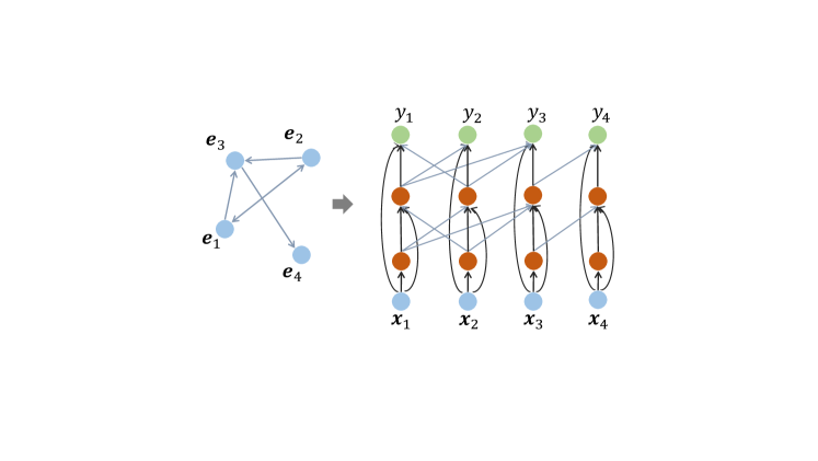
Figure 1: Collective classification with Stacked Learning (SL). (Left): A graph with 4 entities connected by unidirectional and bidirectional links, (Right): SL model for the graph with three steps where $\boldsymbol{x}_{i}$ is the feature vector of entity $\boldsymbol{e}_{i}$. The bidirectional link between $\boldsymbol{e}_{1}$ and $\boldsymbol{e}_{2}$ is modeled as two unidirectional links from $\boldsymbol{e}_{1}$ to $\boldsymbol{e}_{2}$ and vice versa.

Stacked learning (Fig. 1) is a multi-step learning procedure for collective classification (?; ?; ?). At step $t-1$, a classifier is used to predict class probabilities for entity $\boldsymbol{e}_{j}$, i.e., $\boldsymbol{p}_{j}^{t-1}=\left[P^{t-1}\left(y_{j}=1\right),...,P^{t-1}\left(y_{j}=L\right)\right]$. These intermediate outputs are then used as relational features for neighbor classifiers in the next step. In (?), each relation produces one set of contextual features, where all features of the same relation are averaged:

$$\boldsymbol{c}_{ir}^{t}=\frac{1}{\left|\mathcal{N}_{r}(i)\right|}\sum_{j\in\mathcal{N}_{r}(i)}\boldsymbol{p}_{j}^{t-1}$$ (1)

where $\boldsymbol{c}_{ir}^{t}$ is the relational feature vector for relation $r$ at step $t$. The output at step $t$ is predicted as follows

$$P^{t}\left(y_{i}\right)=f^{t}\left(\boldsymbol{x}_{i},\boldsymbol{p}_{i}^{t-1},\left[\boldsymbol{c}_{i1}^{t},\boldsymbol{c}_{i2}^{t}...,\boldsymbol{c}_{iR}^{t}\right]\right)$$ (2)

where $f^{t}$ is the classifier at step $t$. When $t=1$, the model uses local features of entities for classification, i.e., $\boldsymbol{c}_{ir}^{1}=\boldsymbol{0}$ and $\boldsymbol{p}_{i}^{0}=\boldsymbol{0}$. At each step, classifiers are trained sequentially with known-label entities.

3 Column Networks

In this section we present our main contribution, the Column Network ($\mathsf{\mathtt{CLN}}$).

3.1 Architecture

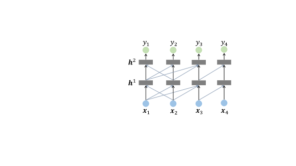
Figure 2: $\mathsf{\mathtt{CLN}}$ for the graph in Fig. 1(Left) with 2 hidden layers ($\boldsymbol{h}^{1}$ and $\boldsymbol{h}^{2}$).

Inspired by the columnar organization in neocortex (?), the $\mathsf{\mathtt{CLN}}$ has one mini-column per entity (or data instance), which is akin to a sensory receptive field. Each column is a feedforward net that passes information from a lower layer to a higher layer of its own, and higher layers of neighbors (see Fig. 2 for a $\mathsf{\mathtt{CLN}}$ that models the graph in Fig.1(Left)). The nature of the inter-column communication is dictated by the relations between the two entities.

Through multiple layers, long-range dependencies are established (see Sec. 3.4 for more in-depth discussion). This somewhat resembles the strategy used in stacked learning as described in Sec. 2.2. The main difference is that in $\mathsf{\mathtt{CLN}}$ the intermediate steps do not output class probabilities but learn higher abstraction of instance features and relational features. As such, our model is end-to-end in the sense that receptive signals are passed from the bottom to the top, and abstract features are inferred along the way. Likewise, the training signals are passed from the top to the bottom.

Denote by $\boldsymbol{x}_{i}\in\mathbb{R}^{M}$ and $\boldsymbol{h}_{i}^{t}\in\mathbb{R}^{K_{t}}$ the input feature vector and the hidden activation at layer $t$ of entity $\boldsymbol{e}_{i}$, respectively. If there is a connection from entity $\boldsymbol{e}_{j}$ to $\boldsymbol{e}_{i}$, $\boldsymbol{h}_{j}^{t-1}$ serves as an input for $\boldsymbol{h}_{i}^{t}$ . Generally, $\boldsymbol{h}_{i}^{t}$ is a non-linear function of $\boldsymbol{h}_{i}^{t-1}$ and previous hidden states of its neighbors:

$$\boldsymbol{h}_{i}^{t}=g\left(\boldsymbol{h}_{i}^{t-1},\boldsymbol{h}_{j_{1}}^{t-1},...,\boldsymbol{h}_{j_{|N(i)|}}^{t-1}\right)$$

where $j\in\mathcal{N}(i)$ and $\boldsymbol{h}_{i}^{0}$ is the input vector $\boldsymbol{x}_{i}$.

We borrow the idea of stacked learning (Sec. 2.2) to handle multiple relations in $\mathsf{\mathtt{CLN}}$. The context of relation $r$ ($r=1,...,R)$ at layer $t$ in Eq. (1) is replaced by

$$\boldsymbol{c}_{ir}^{t}=\frac{1}{\left|\mathcal{N}_{r}(i)\right|}\sum_{j\in\mathcal{N}_{r}(i)}\boldsymbol{h}_{j}^{t-1}$$ (3)

Furthermore, different from stacked learning, the context in $\mathsf{\mathtt{CLN}}$ are abstracted features, i.e., we replace Eq. (2) by

$$\boldsymbol{h}_{i}^{t}=g\left(\boldsymbol{b}^{t}+W^{t}\boldsymbol{h}_{i}^{t-1}+\frac{1}{z}\sum_{r=1}^{R}V_{r}^{t}\boldsymbol{c}_{jr}^{t}\right)$$ (4)

where $W^{t}\in\mathbb{R}^{K^{t}\times K^{t-1}}$ and $V_{r}^{t}\in\mathbb{R}^{K^{t}\times K^{t-1}}$ are weight matrices and $\boldsymbol{b}^{t}$ is a bias vector for some activation function $g$; $z$ is a pre-defined constant which is used to prevent the sum of parameterized contexts from growing too large for complex relations.

At the top layer $T$, for example, the label probability for entity $i$ is given as:

$$P\left(y_{i}=l\right)=\mbox{softmax}\left(\boldsymbol{b}_{l}+W_{l}\boldsymbol{h}_{i}^{T}\right)$$

Remark:

There are several similarities between $\mathsf{\mathtt{CLN}}$ and existing neural network operations. Eq. (3) implements mean-pooling, the operation often seen in CNN. The main difference with the standard CNN is that the mean pooling does not reduce the graph size. This suggests other forms of pooling such as max-pooling or sum-pooling. Asymmetric pooling can also be implemented based on the concept of attention, that is, Eq. (3) can be replaced by:

$$\boldsymbol{c}_{ir}^{t}=\sum_{j\in\mathcal{N}_{r}(i)}\alpha_{j}\boldsymbol{h}_{j}^{t-1}$$

subject to $\sum_{j\in\mathcal{N}_{r}(i)}\alpha_{j}=1$ and $\alpha_{j}\geq 0$.

Eq. (4) implements a convolution. For example, standard 3x3 convolutional kernels in images implement 8 relations: left, right, above, below, above-left, above-right, below-left, below-right. Supposed that the relations are shared between nodes, the $\mathsf{\mathtt{CLN}}$ achieves translation invariance, similar to that in CNN.

3.2 Highway Network as Mini-Column

We now specify the detail of a mini-column, which we implement by extending a recently introduced feedforward net called Highway Network (?). Recall that traditional feedforward nets have a major difficulty of learning with high number of layers. This is due to the nested non-linear structure that prevents the ease of passing information and gradient along the computational path. Highway nets solve this problem by partially opening the gate that lets previous states to propagate through layers, as follows:

$$\boldsymbol{h}^{t}=\boldsymbol{\alpha}_{1}*\tilde{\boldsymbol{h}}^{t}+\boldsymbol{\alpha}_{2}*\boldsymbol{h}^{t-1}$$ (5)

where $\tilde{\boldsymbol{h}}^{t}$ is a nonlinear candidate function of $\boldsymbol{h}^{t-1}$ and where $\boldsymbol{\alpha}_{1},\boldsymbol{\alpha}_{2}\in(\boldsymbol{0},\boldsymbol{1})$ are learnable gates. Since the gates are never shut down completely, data signals and error gradients can propagate very far in a deep net.

For modeling relations, the candidate function $\tilde{\boldsymbol{h}}^{t}$ in Eq. (5) is computed using Eq. (4). Likewise, the gates are modeled as:

$$\boldsymbol{\alpha}_{1} = \sigma\left(\boldsymbol{b}_{\boldsymbol{\alpha}}^{t}+W_{\text{$\boldsymbol{\alpha}$}}^{t}\boldsymbol{h}_{i}^{t-1}+\frac{1}{z}\sum_{r=1}^{R}V_{\boldsymbol{\alpha}r}^{t}\boldsymbol{c}_{jr}^{t}\right)$$ (6)

and $\boldsymbol{\alpha}_{2}=\boldsymbol{1}-\boldsymbol{\alpha}_{1}$ as for compactness (?). Other gating options exists, for example, the $p$-norm gates where $\boldsymbol{\alpha}_{1}^{p}+\boldsymbol{\alpha}_{2}^{p}=\boldsymbol{1}$ for $p>0$ (?).

3.3 Parameter Sharing for Compactness

For feedforward nets, the number of parameters grow with number of hidden layers. In $\mathsf{\mathtt{CLN}}$, the number is multiplied by the number of relations (see Eq. (4)). In highway network implementation of mini-columns, a set of parameters for the gates is used thus doubling the number of parameters (see Eq. (6)). For a deep $\mathsf{\mathtt{CLN}}$ with many relations, the number of parameters may grow faster than the size of training data, leading to overfitting and a high demand of memory. To address this challenge, we borrow the idea of parameter sharing in Recurrent Neural Network (RNN), that is, layers have identical parameters. There has been empirical evidence supporting this strategy in non-relational data (?; ?).

With parameter sharing, the depth of the $\mathsf{\mathtt{CLN}}$ can grow without increasing in model size. This may lead to good performance on small and medium datasets. See Sec. 4 provides empirical evidences.

3.4 Capturing Long-range Dependencies

An important property of our proposed deep $\mathsf{\mathtt{CLN}}$ is the ability to capture long-range dependencies despite only local state exchange as shown in Eqs. (4,6). To see how, let us consider the example in Fig. 2, where $\boldsymbol{x}_{1}$ is modeled in $\boldsymbol{h}_{3}^{1}$ and $\boldsymbol{h}_{3}^{1}$ is modeled in $\boldsymbol{h}_{4}^{2}$, therefore although $\boldsymbol{e}_{1}$ does not directly connect to $\boldsymbol{e}_{4}$ but information of $\boldsymbol{e}_{1}$ is still embedded in $\boldsymbol{h}_{4}^{2}$ through $\boldsymbol{h}_{3}^{1}$. More generally, after $k$ hidden layers, a hidden activation of an entity can contains information of its expanded neighbors of radius $k$. When the number of layers is large, the representation of an entity at the top layer contains not only its local features and its directed neighbors, but also the information of the entire graph. With highway networks, all of these levels of representations are accumulated through layers and used to predict output labels.

3.5 Training with mini-batch

As described in Sec. 3.1, $\boldsymbol{h}_{i}^{t}$ is a function of $\boldsymbol{h}_{i}^{t-1}$ and the previous layer of its neighbors. $\boldsymbol{h}_{i}^{t}$ therefore can contains information of the entire graph if the network is deep enough. This requires full-batch training which is expensive and not scalable. We propose a very simple yet efficient approximation method that allows mini-batch training. For each mini-batch, the neighbor activations are temporarily frozen to scalars, i.e., gradients are not propagated through this “blanket”. After the parameter update, the activations are recomputed as usual. Experiments showed that the procedure did converge and its performance is comparative with the full-batch training method.

4 Experiments and Results

In this section, we report three real-world applications of $\mathsf{\mathtt{CLN}}$ on networked data: software delay estimate, PubMed paper classification and film genre classification.

4.1 Baselines

For comparison, we employed a comprehensive suit of baseline methods which include: (a) those designed for collective classification, and (b) deep neural nets for non-collective classification. For the former, we used NetKit, an open source toolkit for classification in networked data (?). NetKit offers a classification framework consisting of 3 components: a local classifier, a relational classifier and a collective inference method. In our experiments, the local classifier is the Logistic Regression (LR) for all settings; relational classifiers are (i) weighted-vote Relational Neighbor (wvRN), (ii) logistic regression link-based classifier with normalized values (nbD), and (iii) logistic regression link-based classifier with absolute count values (nbC). Collective inference methods include Relaxation Labeling (RL) and Iterative Classification (IC). In total, there are 6 pairs of “relational classifier – collective inference”: wvRN-RL, wvRN-IC, nbD-RL, nbD-IC, nbC-RL and nbC-IC. For each dataset, results of two best settings will be reported.

We also implemented the state-of-the-art collective classifiers following (?; ?; ?): stacked learning with logistic regression (SL-LR) and with random forests (SL-RF).

For deep neural nets, following the latest results in (?; ?), we implemented highway network with shared parameters among layers (HWN-noRel). This is essentially a special case of $\mathsf{\mathtt{CLN}}$ without relational connections.

4.2 Experiment Settings

We report three variants of the $\mathsf{\mathtt{CLN}}$: a basic version that uses standard Feedforward Neural Network as mini-column ($\mathsf{\mathtt{CLN}}$-FNN) and two versions of $\mathsf{\mathtt{CLN}}$-HWN that use highway nets with shared parameters ($\mathsf{\mathtt{CLN}}$-HWN-full for full-batch mode and $\mathsf{\mathtt{CLN}}$-HWN-mini for mini-batch mode, as described in Sections 3.2, 3.3 and 3.5). All neural nets use ReLU in the hidden layers.

Dropout is applied before and after the recurrent layers of $\mathsf{\mathtt{CLN}}$-HWNs and at every hidden layers of $\mathsf{\mathtt{CLN}}$-FNN. Each dataset is divided into 3 separated sets: training, validation and test sets. For hyper-parameter tuning, we search for (i) number of hidden layers: 2, 6, 10, …, 30, (ii) hidden dimensions, and (iii) optimizers: Adam or RMSprop. $\mathsf{\mathtt{CLN}}$-FNN has 2 hidden layers and the same hidden dimension with $\mathsf{\mathtt{CLN}}$-HWN so that the two models have equal number of parameters. The best training setting is chosen by the validation set and the results of the test set are reported. The result of each setting is reported by the mean result of 5 runs. Code for our model can be found on Github

4.3 Software Delay Prediction

This task is to predict potential delay for an issue, which is an unit of task in an iterative software development lifecycle (?). The prediction point is when issue planning has completed. Due to the dependencies between issues, the prediction of delay for an issue must take into account all related issues. We use the largest dataset reported in (?), the JBoss, which contains 8,206 issues. Each issue is a vector of 15 features and connects to other issues through 12 relations (unidirectional such as blocked-by or bidirectional such as same-developer). The task is to predict whether a software issue is at risk of getting delays (i.e., binary classification).

Fig. 3 visualizes $\mathsf{\mathtt{CLN}}$-HWN-full performance with different numbers of layers ranging from 2 to 30 and hidden dimensions from 5, 10 to 20. The F1-score peaks at 10 hidden layers and dimension size of 10.

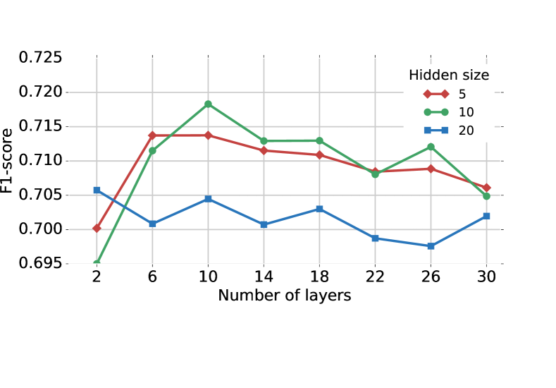
Figure 3: Performance (F1-score) of $\mathsf{\mathtt{CLN}}$-HWN on Software delay prediction task with different numbers of layers and hidden sizes

Table 1 reports the F1-scores of all methods. The two best classifiers in NetKit are wvRN-IC and wvRN-RL. The non-collective HWN-noRel works surprisingly well – almost reaching the performance of the best collective SL-RF with 2 points short. This demonstrates that deep neural nets are highly competitive in this domain, and to the best of our knowledge, this fact has not been established. $\mathsf{\mathtt{CLN}}$-HWN-full beats the best collective-method, the SL-RF by 3.1 points. We lost 0.7% in mini-batch training mode but the gain of training speed was substantial - roughly 6x.

Non-neural	F1	Neural net	F1
wvRN-IC	54.7	HWN-noRel	66.8
wvRN-RL	55.8	$\mathsf{\mathtt{CLN}}$-FNN	70.5
SL-LR	65.3	$\mathsf{\mathtt{CLN}}$-HWN-full	71.9
SL-RF(*)	68.8	$\mathsf{\mathtt{CLN}}$-HWN-mini	71.2

Table 1: Software delay prediction performance. (*) Result reported in (?).

4.4 PubMed Publication Classification

We used the Pubmed Diabetes dataset consisting of 19,717 scientific publications and 44,338 citation links among them. Each publication is described by a TF/IDF weighted word vector from a dictionary which consists of 500 unique words. We conducted experiments of classifying each publication into one of three classes: Diabetes Melitus - Experimental, Diabetes Melitus type 1, and Diabetes Mellitus type 2.

Visualization of hidden layers

We randomly picked 2 samples of each class and visualized their ReLU units activations through 10 layers of the $\mathsf{\mathtt{CLN}}$-HWN (Fig. 4). Interestingly, the activation strength seems to grow with higher layers, suggesting that learn features are more discriminative as they are getting closer to the outcomes. For each class a number of hidden units is turned off in every layer. Figures of samples in the same class have similar patterns while figures of samples from different classes are very different.

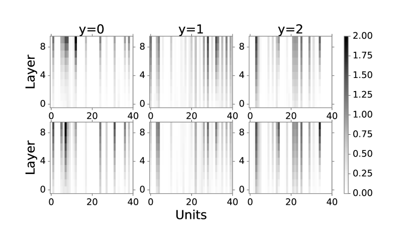
Figure 4: The dynamics of activations of 40 ReLU units through 10 hidden layers of 2x3 samples - each column is for a class.

Classification accuracy

The best setting for $\mathsf{\mathtt{CLN}}$-HWN is with 40 hidden dimensions and 10 recurrent layers. Results are measured in MicroF1-score and MacroF1-score (See Table 2). The non-relational highway net (HWN-noRel) outperforms two best baselines from NetKit. The two version of $\mathsf{\mathtt{CLN}}$-HWN perform best in both F1-score measures.

Method	MicroF1-score	MacroF1-score
wvRN-IC	82.6	81.4
wvRN-RL	82.4	81.2
SL-LR	88.2	87.9
HWN-noRel	87.9	87.9
$\mathsf{\mathtt{CLN}}$-FNN	89.4	89.2
$\mathsf{\mathtt{CLN}}$-HWN-full	89.8	89.6
$\mathsf{\mathtt{CLN}}$-HWN-mini	89.8	89.6

Table 2: Pubmed Diabetes classification results measured by MicroF1-score and MacroF1-score.

4.5 Film Genre Prediction

We used the MovieLens Latest Dataset (?) which consists of 33,000 movies. The task is to predict genres for each movie given plot summary. Local features were extracted from movie plot summary downloaded from IMDB database. After removing all movies without plot summary, the dataset remains 18,352 movies. Each movie is described by a Bag-of-Words vector of 1,000 most frequent words. Relations between movies are (same-actor, same-director). To create a rather balanced dataset, 20 genres are collapsed into 9 labels: (1) Drama, (2) Comedy, (3) Horror + Thriller, (4) Adventure + Action, (5) Mystery + Crime + Film-Noir, (6) Romance, (7) Western + War + Documentary, (8) Musical + Animation + Children, and (9) Fantasy + Sci-Fi. The frequencies of 9 labels are reported in Table 3.

Label	0	1	2	3	4
Freq(%)	46.3	32.5	24.0	19.1	15.9
Label	5	6	7	8
Freq(%)	16.5	14.8	10.4	11.5

Table 3: The frequencies of 9 collapsed labels on Movielens

On this dataset, $\mathsf{\mathtt{CLN}}$-HWNs work best with 30 hidden dimensions and 10 recurrent layers. Table 4 reports the F-scores. The two best settings with NetKit are nbC-IC and nbC-RL. $\mathsf{\mathtt{CLN}}$-FNN performs well on Micro-F1 but fails to improve MacroF1-score of prediction. $\mathsf{\mathtt{CLN}}$-HWN-mini outperforms $\mathsf{\mathtt{CLN}}$-HWN-full by 1.3 points on Macro-F1.

Method	Micro-F1	Macro-F1
nbC-IC	46.6	38.0
nbC-RL	43.5	40.4
SL-LR	53.4	48.9
HWN-noRel	50.8	45.2
$\mathsf{\mathtt{CLN}}$-FNN	54.3	41.8
$\mathsf{\mathtt{CLN}}$-HWN-full	57.4	52.7
$\mathsf{\mathtt{CLN}}$-HWN-mini	57.5	54.1

Table 4: Movie Genre Classification Performance reported in MicroF1 score and MacroF1 score.

Fig. 5 shows why $\mathsf{\mathtt{CLN}}$-FNN performs badly on MacroF1 (MacroF1 is the average of all classes’ F1-scores). While $\mathsf{\mathtt{CLN}}$-FNN works well with balanced classes (in the first three classes, its performance is nearly as good as $\mathsf{\mathtt{CLN}}$-HWN), it fails to handle imbalanced classes (See Table 3 for label frequencies). For example, F1-score is only 5.4% for label 7 and 13.3% for label 8. In contrast, $\mathsf{\mathtt{CLN}}$-HWN performs well on all classes.

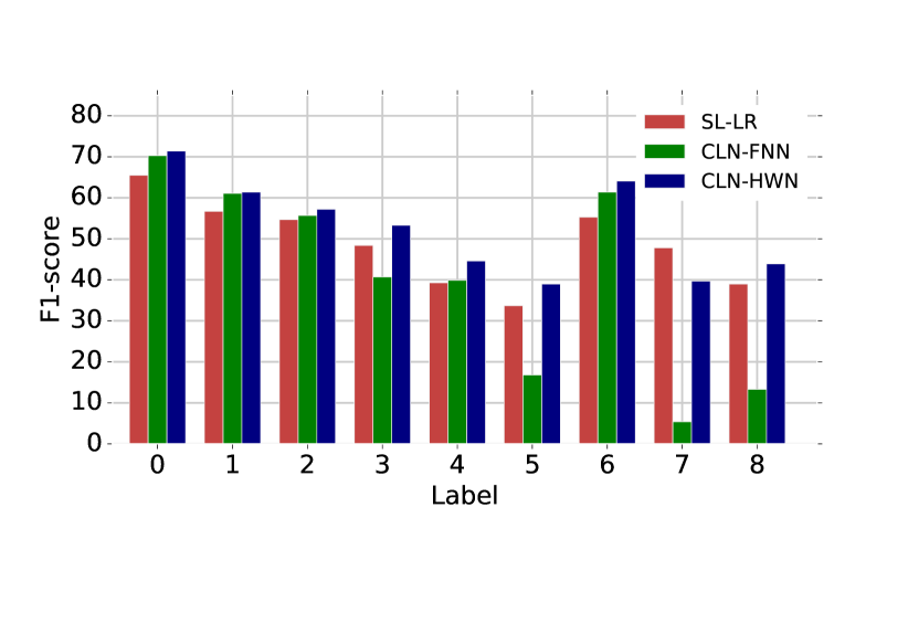
Figure 5: Genre prediction F1-score of SL-LR,$\mathsf{\mathtt{CLN}}$-FNN, $\mathsf{\mathtt{CLN}}$-HWN on each label. Best viewed in color.

5 Related Work

This paper sits at the intersection of two recent independently developed areas: Statistical Relational Learning (SRL) and Deep Learning (DL). Started in the late 1990s, SRL has advanced significantly with noticeable works such as Probabilistic Relational Models (?), Conditional Random Fields (?), Relational Markov Network (?) and Markov Logic Networks (?). Collective classification is a canonical task in SRL, also known in various forms as structured prediction (?) and classification on networked data (?).

Two key components of collective classifiers are relational classifier and collective inference (?). Relational classifier makes use of predicted classes (or class probabilities) of entities from neighbors as features. Examples are wvRN (?), logistic based (?) or stacked graphical learning (?; ?). Collective inference is the task of jointly inferring labels for entities. This is a subject of AI with abundance of solutions including message passing algorithms (?), variational mean-field (?) and discrete optimization (?). Among existing collective classifiers, the closest to ours is stacked graphical learning where collective inference is bypassed through stacking (?; ?). The idea is based on learning a stack of models that take intermediate prediction of neighborhood into account.

The other area is Deep Learning (DL), where the current wave has offered compact and efficient ways to build multilayered networks for function approximation (via feedforward networks) and program construction (via recurrent networks) (?; ?). However, much less attention has been paid to general networked data (?), although there has been work on pairing structured outputs with deep networks (?; ?; ?; ?; ?). Parameter sharing in feedforward networks was recently analyzed in (?; ?). The sharing eventually transforms the networks in to recurrent neural networks (RNNs) with only one input at the first layer. The empirical findings were that the performance is good despite the compactness of the model. Among deep neural nets, the closest to our work is RNCC model (?), which also aims at collective classification using RNNs. There are substantial differences, however. RNCC shuffles neighbors of an entities to a random sequence and uses horizontal RNN to integrate the sequence of neighbors. Ours emphasizes on vertical depth, where parameter sharing gives rise to the vertical RNNs. Ours is conceptually simpler – all nodes are trained simultaneously, not separately as in RNCC.

6 Discussion

This paper has proposed Column Network ($\mathsf{\mathtt{CLN}}$), a deep neural network with an emphasis on fast and accurate collective classification. $\mathsf{\mathtt{CLN}}$ has linear complexity in data size and number of relations in both training and inference. Empirically, $\mathsf{\mathtt{CLN}}$ demonstrates a competitive performance against rival collective classifiers on three real-world applications: (a) delay prediction in software projects, (b) PubMed Diabetes publication classification and (c) film genre classification.

As the name suggests, $\mathsf{\mathtt{CLN}}$ is a network of narrow deep networks, where each layer is extended to incorporate as input the preceding neighbor layers. It somewhat resembles the columnar structure in neocortex (?), where each narrow deep network plays a role of a mini-column. We wish to emphasize that although we use highway networks in actual implementation due to its excellent performance (?; ?; ?), any feedforward networks can be potentially be used in our architecture. When parameter sharing is used, the feedforward networks become recurrent networks, and $\mathsf{\mathtt{CLN}}$ becomes a network of interacting RNNs. Indeed, the entire network can be collapsed into a giant feedforward network with $n-n$ input/output mappings. When relations are shared among all nodes across the network, $\mathsf{\mathtt{CLN}}$ enables translation invariance across the network, similar to those in CNN. However, the $\mathsf{\mathtt{CLN}}$ is not limited to a single network with shared relations. Alternatively, networks can be IID according to some distribution and this allows relations to be specific to nodes.

There are open rooms for future work. One extension is to learn the pooling operation using attention mechanisms. We have considered only homogeneous prediction tasks here, assuming instances are of the same type. However, the same framework can be easily extended to multiple instance types.

References

- [Belanger and McCallum 2016] Belanger, D., and McCallum, A. 2016. Structured prediction energy networks. ICML.
- [Choetkiertikul et al. 2015] Choetkiertikul, M.; Dam, H. K.; Tran, T.; and Ghose, A. 2015. Predicting delays in software projects using networked classification. In 30th IEEE/ACM International Conference on Automated Software Engineering.
- [Dietterich et al. 2008] Dietterich, T. G.; Domingos, P.; Getoor, L.; Muggleton, S.; and Tadepalli, P. 2008. Structured machine learning: the next ten years. Machine Learning 73(1):3–23.
- [Do, Arti, and others 2010] Do, T.; Arti, T.; et al. 2010. Neural conditional random fields. In International Conference on Artificial Intelligence and Statistics, 177–184.
- [Domke 2013] Domke, J. 2013. Structured learning via logistic regression. In Advances in Neural Information Processing Systems, 647–655.
- [Getoor and Sahami 1999] Getoor, L., and Sahami, M. 1999. Using probabilistic relational models for collaborative filtering. In Workshop on Web Usage Analysis and User Profiling (WEBKDD’99).
- [Harper and Konstan 2016] Harper, F. M., and Konstan, J. A. 2016. The movielens datasets: History and context. ACM Transactions on Interactive Intelligent Systems (TiiS) 5(4):19.
- [Hinton 2002] Hinton, G. 2002. Training products of experts by minimizing contrastive divergence. Neural Computation 14:1771–1800.
- [Kou and Cohen 2007] Kou, Z., and Cohen, W. W. 2007. Stacked Graphical Models for Efficient Inference in Markov Random Fields. In SDM, 533–538. SIAM.
- [Lafferty, McCallum, and Pereira 2001] Lafferty, J.; McCallum, A.; and Pereira, F. 2001. Conditional random fields: Probabilistic models for segmenting and labeling sequence data. In Proceedings of the International Conference on Machine learning (ICML), 282–289.
- [LeCun, Bengio, and Hinton 2015] LeCun, Y.; Bengio, Y.; and Hinton, G. 2015. Deep learning. Nature 521(7553):436–444.
- [Liao and Poggio 2016] Liao, Q., and Poggio, T. 2016. Bridging the gaps between residual learning, recurrent neural networks and visual cortex. arXiv preprint arXiv:1604.03640.
- [Macskassy and Provost 2007] Macskassy, S., and Provost, F. 2007. Classification in networked data: A toolkit and a univariate case study. The Journal of Machine Learning Research 8:935–983.
- [Mnih et al. 2015] Mnih, V.; Kavukcuoglu, K.; Silver, D.; Rusu, A. A.; Veness, J.; Bellemare, M. G.; Graves, A.; Riedmiller, M.; Fidjeland, A. K.; Ostrovski, G.; et al. 2015. Human-level control through deep reinforcement learning. Nature 518(7540):529–533.
- [Monner, Reggia, and others 2013] Monner, D. D.; Reggia, J.; et al. 2013. Recurrent neural collective classification. Neural Networks and Learning Systems, IEEE Transactions on 24(12):1932–1943.
- [Mountcastle 1997] Mountcastle, V. B. 1997. The columnar organization of the neocortex. Brain 120(4):701–722.
- [Neville and Jensen 2000] Neville, J., and Jensen, D. 2000. Iterative classification in relational data. In Proc. AAAI-2000 Workshop on Learning Statistical Models from Relational Data, 13–20.
- [Neville and Jensen 2007] Neville, J., and Jensen, D. 2007. Relational dependency networks. Journal of Machine Learning Research 8(Mar):653–692.
- [Opper and Saad 2001] Opper, M., and Saad, D. 2001. Advanced mean field methods: Theory and practice. Massachusetts Institute of Technology Press (MIT Press).
- [Pearl 1988] Pearl, J. 1988. Probabilistic Reasoning in Intelligent Systems: Networks of Plausible Inference. San Francisco, CA: Morgan Kaufmann.
- [Pham et al. 2016] Pham, T.; Tran, T.; Phung, D.; and Venkatesh, S. 2016. Faster training of very deep networks via p-norm gates. ICPR’16.
- [Richardson and Domingos 2006] Richardson, M., and Domingos, P. 2006. Markov logic networks. Machine Learning 62:107–136.
- [Schmidhuber 2015] Schmidhuber, J. 2015. Deep learning in neural networks: An overview. Neural Networks 61:85–117.
- [Sen et al. 2008] Sen, P.; Namata, G.; Bilgic, M.; Getoor, L.; Galligher, B.; and Eliassi-Rad, T. 2008. Collective classification in network data. AI magazine 29(3):93.
- [Srivastava, Greff, and Schmidhuber 2015] Srivastava, R. K.; Greff, K.; and Schmidhuber, J. 2015. Training very deep networks. In Advances in neural information processing systems, 2377–2385.
- [Sutton and McCallum 2007] Sutton, C., and McCallum, A. 2007. Piecewise pseudolikelihood for efficient CRF training. In Proceedings of the International Conference on Machine Learning (ICML), 863–870.
- [Taskar, Pieter, and Koller 2002] Taskar, B.; Pieter, A.; and Koller, D. 2002. Discriminative probabilistic models for relational data. In Proceedings of the 18th Conference on Uncertainty in Artificial Intelligence (UAI), 485–49. Morgan Kaufmann.
- [Tompson et al. 2014] Tompson, J. J.; Jain, A.; LeCun, Y.; and Bregler, C. 2014. Joint training of a convolutional network and a graphical model for human pose estimation. In Advances in neural information processing systems, 1799–1807.
- [Tran and Dinh Phung 2014] Tran, T., and Dinh Phung, S. V. 2014. Tree-based Iterated Local Search for Markov Random Fields with Applications in Image Analysis. Journal of Heuristics DOI:10.1007/s10732-014-9270-1.
- [Tran, Phung, and Venkatesh 2016] Tran, T.; Phung, D.; and Venkatesh, S. 2016. Neural choice by elimination via highway networks. Trends and Applications in Knowledge Discovery and Data Mining, Lecture Notes in Computer Science 9794:15–25.
- [Yu, Wang, and Deng 2010] Yu, D.; Wang, S.; and Deng, L. 2010. Sequential labeling using deep-structured conditional random fields. Selected Topics in Signal Processing, IEEE Journal of 4(6):965–973.
- [Zheng et al. 2015] Zheng, S.; Jayasumana, S.; Romera-Paredes, B.; Vineet, V.; Su, Z.; Du, D.; Huang, C.; and Torr, P. H. 2015. Conditional random fields as recurrent neural networks. In Proceedings of the IEEE International Conference on Computer Vision, 1529–1537.