KEK-TH-1934
The complex Langevin analysis of spontaneous symmetry breaking induced by complex fermion determinant
Yuta Itoa111 E-mail address : yito@post.kek.jp and Jun Nishimuraab222 E-mail address : jnishi@post.kek.jp
aKEK Theory Center,
High Energy Accelerator Research Organization,
1-1 Oho, Tsukuba, Ibaraki 305-0801, Japan
bGraduate University for Advanced Studies (SOKENDAI),
1-1 Oho, Tsukuba, Ibaraki 305-0801, Japan
abstract
In many interesting physical systems, the determinant which appears from integrating out fermions becomes complex, and its phase plays a crucial role in the determination of the vacuum. An example of this is QCD at low temperature and high density, where various exotic fermion condensates are conjectured to form. Another example is the Euclidean version of the type IIB matrix model for 10d superstring theory, where spontaneous breaking of the SO(10) rotational symmetry down to SO(4) is expected to occur. When one applies the complex Langevin method to these systems, one encounters the singular-drift problem associated with the appearance of nearly zero eigenvalues of the Dirac operator. Here we propose to avoid this problem by deforming the action with a fermion bilinear term. The results for the original system are obtained by extrapolations with respect to the deformation parameter. We demonstrate the power of this approach by applying it to a simple matrix model, in which spontaneous symmetry breaking from SO(4) to SO(2) is expected to occur due to the phase of the complex fermion determinant. Unlike previous work based on a reweighting-type method, we are able to determine the true vacuum by calculating the order parameters, which agree with the prediction by the Gaussian expansion method.
1 Introduction
The sign problem is a notorious technical problem that occurs in applying Monte Carlo methods to a system with a complex action . The importance sampling cannot be applied as it is since the integrand of the partition function cannot be regarded as a Boltzmann weight. If one uses the absolute value for generating configurations and treats the phase factor as a part of the observable, huge cancellations occur among configurations, and the required statistics grows exponentially with the system size. This problem occurs in various interesting systems in particle physics such as finite density QCD, gauge theories with a theta term or a Chern-Simons term, chiral gauge theories and supersymmetric theories.
The complex Langevin method (CLM) [1, 2] is a promising approach to such complex-action systems, which may be regarded as an extension of the stochastic quantization based on the Langevin equation. The dynamical variables of the original system are naturally complexified, and the observables as well as the drift term are extended holomorphically by analytic continuation. It is known that the CLM works beautifully in highly nontrivial cases [3, 4, 5, 6], while it gives simply wrong results in the other cases [7, 8, 9, 10].
In the past several years, significant progress has been made in theoretical understanding of the method and the conditions for justifying the CLM. First it was realized that the probability distribution of the complexified dynamical variables has to fall off fast enough in the imaginary directions of the configuration space [11, 12]. In order to satisfy this condition, a new technique called gauge cooling [13] was proposed. Using the gauge cooling, the CLM has been successfully applied to finite density QCD333There are also attempts to apply the CLM to the real-time dynamics [14, 15, 16, 17] and to Yang-Mills theory with a theta term [18, 19]. either with heavy quarks [13] or at high temperature [20]. An explicit justification of the gauge cooling has been provided recently [21] extending the argument for justification of the CLM without gauge cooling [11, 12].
It was known for some time that the CLM gives wrong results also when the determinant that appears from integrating out fermions takes values close to zero during the complex Langevin simulation. This was first realized in the Random Matrix Theory for finite density QCD [22, 23] and confirmed also in effective Polyakov line models [24]. In these papers, it was speculated that the problem occurs due to the ambiguity associated with the branch cut in the logarithm of the complex fermion determinant, which appears in the effective action. On the other hand, ref. [25] pointed out that the singular drift term one obtains from the fermion determinant breaks holomorphy, which plays a crucial role in justifying the method.
A theoretical understanding of this problem and a possible cure have been given recently. First it was pointed out in ref. [26] that the branch cut cannot be the cause of the problem since the CLM can be formulated solely in terms of the weight without ever having to refer to the action . Indeed it was found that a similar problem can occur when the action has pole singularities instead of logarithmic singularities. In the same paper, it was shown that the probability distribution of the complexified variables has to fall off fast enough near the singularities of the drift term, based on the argument for justification in ref. [11, 12]. It was then proposed [27, 28] that the gauge cooling can be used to satisfy this condition as well with an appropriate choice of the complexified gauge transformation. A test in the Random Matrix Theory shows that the gauge cooling indeed solves the singular-drift problem unless the quark mass becomes too small.
In ref. [29], the argument for justification with or without gauge cooling was revisited. In particular, it was pointed out that the expectation values of time-evolved observables, which play a crucial role in the argument, can be ill-defined. Taking this into account, it was shown that the CLM can be justified if the probability distribution of the drift term falls off exponentially or faster at large magnitude. This condition serves as a useful criterion, which tells us clearly whether the results obtained by the CLM are trustable or not.
In this paper, we focus on the singular-drift problem that occurs in a system with a complex fermion determinant. In many such systems, the phase of the fermion determinant is expected to play a crucial role in the determination of the vacuum. An example of this is finite density QCD at low temperature and high density, where various exotic fermion condensates are conjectured to form (See ref. [30], for instance.). Another example is the Euclidean version of the type IIB matrix model [31] for 10d superstring theory, where the SO(10) rotational symmetry is conjectured to be spontaneously broken [32, 33, 34, 35]. When one applies the CLM to these systems, the singular-drift problem occurs due to the appearance of eigenvalues of the Dirac operator close to zero. We propose to avoid this problem by deforming the action with a fermion bilinear term and extrapolating its coefficient to zero. The fermion bilinear term should be chosen in such a way that the nearly zero eigenvalues of the Dirac operator are avoided and yet the vacuum of the system is minimally affected.
We test this idea in an SO(4)-symmetric matrix model with a Gaussian action and a complex fermion determinant, in which spontaneous breaking of SO(4) symmetry is expected to occur due to the phase of the determinant [36]. This model was studied previously by the Gaussian expansion method (GEM) [37] and the spontaneous breaking of the SO(4) symmetry down to SO(2) was suggested by comparing the free energy for the SO(2)-symmetric vacuum and the SO(3)-symmetric vacuum. The same model was studied also by Monte Carlo simulation using the factorization method444This is a kind of reweighting method that attempts to solve the so-called overlap problem, which is an important part of the complex-action problem. While the original version was proposed in ref. [35], the importance of constraining observables which are strongly correlated with the phase of the determinant was recognized later in refs. [38, 39]., and the order parameters obtained by the GEM were reproduced for both the SO(2)-symmetric vacuum and the SO(3)-symmetric vacuum [38, 39]. However, the comparison of free energy for the two vacua suffered from too much uncertainty to make a definite conclusion on the true vacuum by this approach.
When one applies the CLM to this system, the singular-drift problem is actually severe because the fermionic part of the model is essentially an exactly “massless” system. Indeed, it turns out that the gauge cooling proposed in refs. [27, 28] is not sufficient to solve this problem in the case at hand. Following the idea described above, we therefore add a fermion bilinear term, which breaks the SO(4) symmetry minimally, down to SO(3). The results of the CLM show that the SO(3) symmetry of the deformed model is broken spontaneously to SO(2). Extrapolating the deformation parameter to zero, we find that the SO(4) symmetry of the original matrix model is broken spontaneously to SO(2) and that the order parameters thus obtained agree well with the prediction obtained by the GEM. We also try another type of the fermion bilinear term for the deformation and show that the final results obtained after the extrapolations remain the same, which supports the validity of our analysis. Note that we are able to determine the true vacuum directly without having to compare the free energy for each vacuum preserving different amount of rotational symmetry.
In order to probe the spontaneous symmetry breaking (SSB), we need to introduce an O() symmetry breaking term in the action, on top of the deformation described above, and send to zero after taking the large- limit. The singular-drift problem occurs at small even for the deformed model. Here, the criterion for correct convergence proposed recently [29] turns out to be useful since it tells us which data are free from the singular-drift problem and hence can be trusted. Indeed, we find that the data points in the reliable region can be fitted nicely by an expected asymptotic behavior, while the data points in the unreliable region deviate from the fitting curve. We hope that our strategy to overcome the singular-drift problem enables the application of the CLM to the type IIB matrix model and to finite density QCD at low temperature and high density.
The rest of this paper is organized as follows. In section 2, we define the SO(4)-symmetric matrix model and briefly review the results obtained by the previous approaches. In section 3, we explain how we apply the CLM to the SO(4)-symmetric matrix model. In particular, we deform the action with a fermion bilinear term, which enables us to investigate the SSB without suffering from the singular-drift problem. In section 4, we present the results of our analysis. In particular, we extrapolate the deformation parameter to zero, and confirm that the SSB from SO(4) to SO(2) indeed occurs in this model. The order parameters thus obtained are in good agreement with the prediction of the GEM. Section 5 is devoted to a summary and discussions. In appendix A we give the details on how we determine the region of validity of the CLM, which is useful in making the extrapolations. In appendix B, we present the results obtained by deforming the action with another type of the fermion bilinear term, which turn out to be consistent with the ones obtained in section 4.
2 Brief review of the SO(4)-symmetric matrix model
The SO(4)-symmetric matrix model investigated in this paper is defined by the partition function [36]
| (2.1) |
where the bosonic part and the fermionic part of the action is given, respectively, as
| (2.2) | |||||
| (2.3) |
Here we have introduced Hermitian matrices , which are bosonic, and copies of -dimensional column vectors and row vectors , which are fermionic. The matrices are the gamma matrices in 4d Euclidean space after Weyl projection, which are defined by
using the Pauli matrices (). The model has an SO(4) symmetry, under which transforms as a vector, whereas and transform as Weyl spinors. Also, the model has an SU() symmetry, under which the dynamical variables transform as
| (2.4) |
where .
Integrating out the fermionic variables for each , one obtains the determinant of the Dirac operator
| (2.5) |
which is complex in general. Thus, the partition function (2.1) can be rewritten as
| (2.6) |
It was speculated that the SO(4) rotational symmetry of the model is spontaneously broken in the large- limit with fixed due to the effect of the phase of the determinant [36]. In the phase-quenched model, which is defined by omitting the phase of the fermion determinant, the SSB was shown not to occur by Monte Carlo simulation [39]. We may therefore say that the SSB, if it really occurs, should be induced by the phase of the fermion determinant. Throughout this paper, we consider the case, which corresponds to .
In order to see the SSB, we introduce an SO(4)-breaking mass term
| (2.7) |
in the action, where
| (2.8) |
and define the order parameters for the SSB by the expectation values of
| (2.9) |
where no sum over is taken. Due to the ordering (2.8), the expectation values obey
| (2.10) |
at finite . Taking the large- limit and then sending to zero afterwards, the expectation values () may not take the same value. In that case, we can conclude that the SSB occurs.
Explicit calculations based on the GEM were carried out assuming that the SO(4) symmetry is broken down either to SO(2) or to SO(3) [37]. For , the order parameters are given by
| (2.11) | ||||
| (2.12) |
The free energy was calculated in each vacuum, and the SO(2)-symmetric vacuum was found to have a lower value.
Monte Carlo simulation of this model is difficult due to the sign problem caused by the complex fermion determinant. Among various reweighting-type methods, the factorization method [35] turned out to be particularly useful in the present case. Assuming that the SO(4) symmetry is spontaneously broken down either to SO(2) or to SO(3), the results of the GEM (2.11) and (2.12) were reproduced [38, 39]. However, the calculation of the free energy difference had large uncertainties, and it was not possible to determine which vacuum is actually realized using this approach.
3 Application of the CLM to the SO(4)-symmetric matrix model
In this section, we explain how we apply the CLM to the SO(4)-symmetric matrix model (2.1). Including the symmetry breaking term (2.7), we can write the partition function as
| (3.1) |
The drift term that appears in the Langevin equation is given by
| (3.2) | ||||
| (3.3) |
as a function of the Hermitian matrices . Note that the second term in (3.3) is not Hermitian in general corresponding to the fact that the fermion determinant is complex. Thus, the application of the idea of stochastic quantization naturally leads us to complexifying the dynamical variables, which amounts to regarding the Hermitian matrices as general complex matrices . Accordingly, the definition of the drift term (3.3) is extended to general complex matrices by analytic continuation. Then we consider the fictitious-time evolution of the general complex matrices described by the discretized version of the complex Langevin equation
| (3.4) |
where is an Hermitian matrix generated with the probability proportional to . The expectation values of the observables (2.9) can be calculated as
| (3.5) |
where represents the time required for thermalization and should be large enough to achieve good statistics.
In order to justify the CLM, the probability distribution of the drift term (3.3) measured during the complex Langevin simulation should fall off exponentially or faster at large magnitude [29]. In the present model, this condition can be violated for two reasons. First, the first term in (3.3) can be large when the configuration becomes too far from Hermitian. Second, the second term in (3.3) can be large when the Dirac operator has an eigenvalue close to zero.
In order to avoid the first problem, we use the gauge cooling [13]. Note that the original theory (3.1) has the symmetry with , under which the drift term (3.3) transforms covariantly as and the observables (2.9) are invariant. Upon complexifying the variables, the symmetry property of the drift term and the observables enhances to with . Using this fact, we can implement the gauge cooling procedure [13] in the Langevin process as
| (3.6) | ||||
| (3.7) |
where the transformation matrix is chosen appropriately as a function of the configuration before gauge cooling. (See refs. [21, 29] for explicit justification.)
In order to keep the matrices close to Hermitian, we define the Hermiticity norm
| (3.8) |
which measures the deviation of from a Hermitian configuration, and choose the transformation in (3.6) in such a way that the norm is minimized. In practice, this is done by using the steepest descent method as follows.
Let us consider an infinitesimal transformation
| (3.9) |
where traceless Hermitian matrices are the generators of normalized as . Since the norm (3.8) is invariant under , we restrict the infinitesimal parameters to be real. Under the infinitesimal transformation, we have
| (3.10) |
Therefore, the change of the Hermiticity norm (3.8) becomes
| (3.11) |
from which the gradient of the norm is obtained as
| (3.12) |
Using this , we consider a finite transformation
| (3.13) |
where the real positive parameter is chosen in such a way that the Hermiticity norm (3.8) is approximately minimized. We repeat this procedure until the norm (3.8) stops decreasing within certain accuracy.
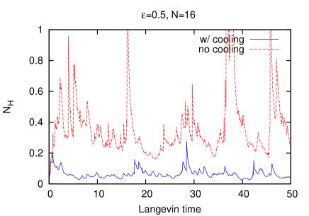
In Fig. 1, we plot the history of the Hermiticity norm (3.8) measured during the Langevin simulation for and . Here and henceforth, the parameters in the SO(4)-breaking term (2.7) are chosen as
| (3.14) |
and the Langevin step-size is chosen as unless stated otherwise. We find that the gauge cooling keeps the Hermiticity norm well under control.
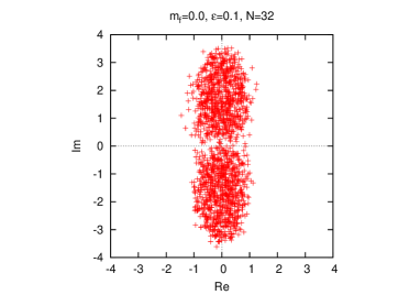
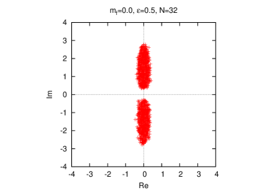
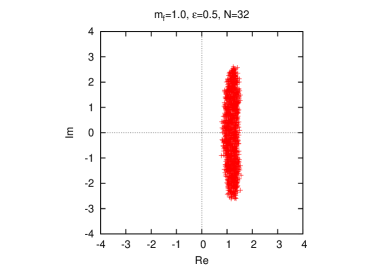
Next we turn to the second problem, which is associated with the eigenvalues of the Dirac operator close to zero. In Fig. 2, we plot the eigenvalue distribution of the Dirac operator obtained during the complex Langevin simulation for (Left) and (Right) with . We find that there are many eigenvalues close to zero for , but not for . This suggests that there is some critical , below which the results of the CLM cannot be trusted because of the singular-drift problem. It turns out that the extrapolation to is rather difficult in this situation.
In order to avoid this problem, we add a fermion bilinear term
| (3.15) |
to the action (2.3). The partition function of the deformed model is defined as
| (3.16) |
Note that the extra fermion bilinear term explicitly breaks the SO(4) symmetry of the original model (2.1). Here we choose the parameters in such a way that the SO(4) symmetry is broken minimally. Taking account of the ordering (2.10), we can preserve an SO(3) symmetry at by choosing
| (3.17) |
We can then ask whether the SO(3) symmetry of this deformed model is spontaneously broken in the large- limit.
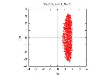
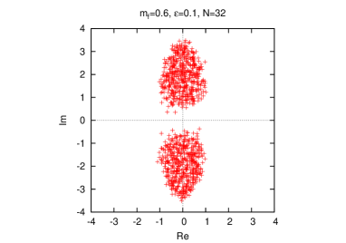
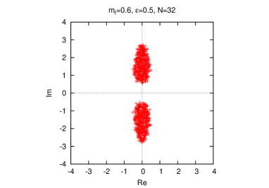
In Fig. 3, we plot the eigenvalue distribution of the Dirac operator (3.16) obtained during the complex Langevin simulation of the deformed model for (Left) and (Right) with and . We find that the distribution is shifted in the real direction. This is understandable since, at large , the eigenvalue distribution of the Dirac operator would be distributed around . As a result, the distribution avoids the singularity even for in contrast to the undeformed () case. Therefore, we can extrapolate to zero using data obtained with smaller for finite . Eventually, we extrapolate the deformation parameter to zero, and compare the results with the prediction (2.11) obtained by the GEM for the original model.
4 Results of our analysis
In this section, we present our results obtained by the CLM as described in the previous section. Let us recall that we have introduced an O() mass term (2.7) for the bosonic matrices, which breaks the SO(4) symmetry explicitly. In order to probe the SSB, we need to take the large- limit with fixed , and then make an extrapolation to .
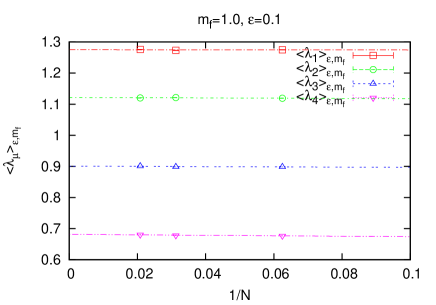
In Fig. 4, the expectation values () obtained for , 32, 48 with and are plotted against , where the data can be fitted nicely to straight lines. Thus we can extrapolate the expectation values to for each and . In what follows, we assume that the large- limit is already taken in this way.
Next we would like to make an extrapolation to . For that purpose, it is convenient to consider the ratio
| (4.1) |
This is motivated from the fact that the mass term (2.7) tends to make all the expectation values smaller than the value to be obtained in the limit. By taking the ratio (4.1), the finite effects are canceled by the denominator, and the extrapolation to becomes easier. Since is a parameter in the action (2.7), the expectation values and hence the ratios (4.1) can be expanded in a power series with respect to . By taking the ratios, the coefficients of higher order terms become smaller, and the truncation of the series becomes valid for a wider range of .
In Fig. 5, we plot the ratio (4.1) against for (Top-Left), 0.8 (Top-Right), 0.6 (Bottom-Left) and 0.4 (Bottom-Right). The data obtained at small suffer from the singular-drift problem, and hence cannot be trusted. Here the condition for justifying the CLM proposed recently in ref. [29] turns out to be useful since it enables us to determine the range of validity as we explain in appendix A. Taking this into account, we fit the data in Fig. 5 to the quadratic form using the fitting range given in Table 1, where we also present the extrapolated values. We find for each value of that and approach the same value in the limit, while the others approach smaller values. This implies that the SSB from SO(3) to SO(2) occurs in the deformed model.


In Fig. 6, we plot the extrapolated values obtained in this way against . We find that our results within can be nicely fitted to the quadratic behavior, which is motivated by a power series expansion of the expectation values with respect to .555The odd order terms in do not appear due to the symmetry of the expectation values. Extrapolating to zero, we obtain for , which shows that the SO(4) symmetry of the undeformed model () is spontaneously broken down to SO(2). Moreover, using an exact result [36] for the present case, we obtain
| (4.2) |
which agree well with the results (2.11) obtained by the GEM. Here we emphasize that in the GEM, the true vacuum was determined by comparing the free energy obtained for the SO() vacuum and the SO() vacuum. In contrast, the CLM enables us to determine the true vacuum directly without having to compare the free energy for different vacua.

As a further consistency check, we repeat the same analysis with a different choice of the deformation parameter in (3.16) instead of (3.17). We find that the results obtained after the extrapolation turn out to be consistent with the ones obtained above. See appendix B for the details.
| fitting range | extrapolated value | ||
|---|---|---|---|
| 1.0 | 1 | 0.2673(20) | |
| 2 | 0.2685(18) | ||
| 3 | 0.2487(09) | ||
| 4 | 0.2144(32) | ||
| 0.8 | 1 | 0.2806(21) | |
| 2 | 0.2815(13) | ||
| 3 | 0.2413(11) | ||
| 4 | 0.1934(24) | ||
| 0.6 | 1 | 0.3014(24) | |
| 2 | 0.2997(13) | ||
| 3 | 0.2298(10) | ||
| 4 | 0.1669(19) | ||
| 0.4 | 1 | 0.3144(20) | |
| 2 | 0.3125(11) | ||
| 3 | 0.2183(07) | ||
| 4 | 0.1495(08) |
5 Summary and discussion
In this paper, we have shown that the CLM can be successfully applied to a matrix model, in which the SSB of SO(4) is expected to occur due to the phase of the complex fermion determinant. The SSB does not occur if the phase is quenched, which implies that it is extremely hard to investigate this phenomenon by reweighting-based Monte Carlo methods. In the factorization method, for instance, one introduces a constraint with some parameters and extremizes the free energy with respect to these parameters. While this has been done successfully in refs. [38, 39], the comparison of the free energy for the SO(2) and SO(3) vacua turns out to be subtle and a definite conclusion on the true vacuum was not reached. In contrast, we have shown by the CLM that the SSB from SO(4) down to SO(2) occurs as predicted by the GEM.
For the success of the CLM, it was crucial to overcome the singular-drift problem associated with the appearance of nearly zero eigenvalues of the Dirac operator. The gauge cooling was used to suppress the excursions in the imaginary directions, but the singular-drift problem in the present case was too severe to be solved by the gauge cooling. This is understandable because the fermionic variables are exactly “massless” in the present case. Our strategy to overcome the singular-drift problem was to deform the Dirac operator in such a way that the singular-drift problem is avoided while maintaining the qualitative feature of the vacuum as much as possible. On top of this, we have to introduce an O() symmetry breaking term to probe the SSB, which should be removed after taking the large- limit. In making the extrapolations, the criterion for correct convergence proposed in ref. [29] turns out to be useful since it tells us the range of parameters for which the CLM is free from the singular-drift problem and the results are trustable. The order parameters obtained after extrapolating the deformation parameter to zero turn out to be consistent with the prediction by the GEM.
We have actually tried two types of deformation to avoid the singular-drift problem and confirmed that the extrapolated results agree with each other within fitting errors. While this confirms the validity of the extrapolations to some extent, we cannot exclude the possibility that something dramatic happens when the deformation parameter approaches zero. Let us recall, however, that the singular-drift problem can occur at some point in the parameter space even if the system itself does not undergo any dramatic change. For instance, in QCD at finite density, the singular-drift problem is anticipated to occur at the quark chemical potential , where is the pion mass, but the first order transition to the phase of nuclear matter occurs at , where is the nucleon mass. Nothing really happens in the wide parameter range . This example clearly shows that the singular-drift problem has more to do with the methodology rather than the physics of the system to be investigated.
The CLM with the proposed strategy can be directly applied to the type IIB matrix model, which is conjectured to be a nonperturbative formulation of type IIB superstring theory in ten dimensions [31]. While the SO(10) symmetry of the model is expected to be spontaneously broken down to SO(4) for consistency with our 4d space-time, the GEM predicts that it is spontaneously broken down to SO(3) rather than SO(4) [40]. It would be interesting to investigate this issue using the CLM extending the present work.
We consider that the same strategy would be useful also in applying the CLM to finite density QCD at low temperature and high density, where various exotic condensates are speculated to form [30] due to the complex fermion determinant. In this case, one can deform the Dirac operator by switching on the corresponding fermion bilinear term without disturbing the vacuum significantly. Now that we have a useful criterion [29] for justifying the CLM, we can try possible deformations and see whether any of them allows us to extrapolate the deformation parameter to zero within the region of validity.
Acknowledgements
The authors would like to thank K.N. Anagnostopoulos, T. Azuma, K. Nagata, S.K. Papadoudis and S. Shimasaki for valuable discussions. Y. I. is supported by JICFuS. J. N. is supported in part by Grant-in-Aid for Scientific Research (No. 23244057 and 16H03988) from Japan Society for the Promotion of Science.
Appendix A How to determine the region of validity
In this appendix, we explain how to determine the region of validity of the CLM. When the symmetry breaking parameter becomes small, the singular-drift problem occurs and the results obtained by the CLM can no longer be trusted. In order to make extrapolations, it is important to determine the value of , below which the results become unreliable. Here we use the criterion based on the argument for justifying the CLM [29]. For that, we calculate the magnitude of the drift term for each configuration and obtain its probability distribution. If the tail of the distribution falls off exponentially or faster, we can trust the results obtained with those simulation parameters. We find that the finite step-size effects can modify the tail of the distribution significantly without changing the expectation values . In order to make the plots in this section, we therefore have to decrease the step-size when it turns out to be necessary.
Let us define the magnitude of the drift term by
| (A.1) |
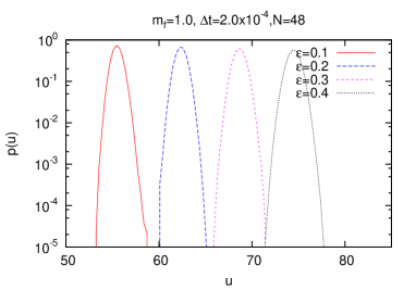
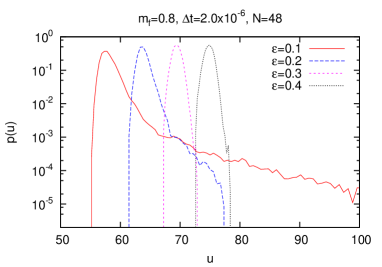
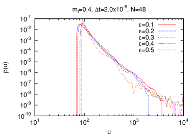
where is the drift term defined by (3.3). Then, we define the probability distribution with the normalization . In Fig. 7, we plot against in the log scale for various with and . We find that falls off exponentially or faster for all the . Thus, we can trust the results obtained in this region.
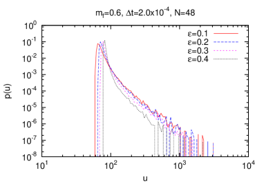
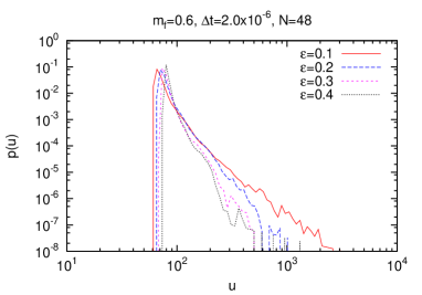
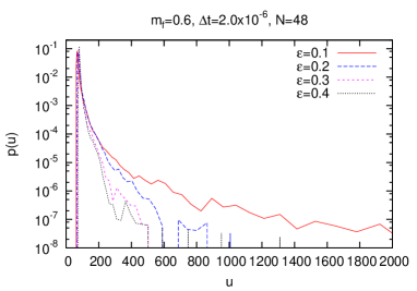
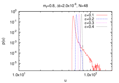
In Fig. 8, we show a log-log plot (Left) and a semi log plot (Right) of the distribution for various with and . Since the drift term can become fairly large for , we decrease the Langevin step-size to in order to probe the tail of the distribution correctly. We find that the distribution falls off exponentially or faster for , but a power-law tail develops for . Therefore, we can trust the data for , but not the ones at .
In Fig. 9, we show a log-log plot of for various with and . Here the drift term tends to become even larger than in the case, and we have to investigate the tail of the distribution more carefully. We therefore present the results obtained for two Langevin step-size, (Left) and (Right). Indeed, we find that the behavior of the tail seems to change qualitatively by decreasing the step-size. In Fig. 10, we show a semi-log plot for , which suggests that the tail of the distribution falls off exponentially for , but not for . The result for is marginal. We may therefore trust the results for .
In Fig. 11, we show a log-log plot of for various with and . Here we have decreased the Langevin step-size to , but the tail of the distribution still follows a power law for all values of within the region. However, the comparison of the two plots in Fig. 9 suggests a possibility that the step-size should be decreased further to see the behavior of the tail correctly. Thus for the case alone, we had to determine the lower end of the fitting range empirically from the plausibility of the fit to the quadratic behavior. Even if we omit the point in Fig. 5, the values obtained by extrapolations to remain almost the same.
Appendix B Results for another type of the fermion bilinear term
In this appendix, we present the results obtained by choosing the deformation parameters in (3.16) as
| (B.1) |
instead of (3.17). Taking into account the ordering (2.10), we can preserve only an SO(2) symmetry with this choice.
In Fig. 12, we plot the eigenvalue distribution of the Dirac operator (3.16) for (Left) and (Right) with and . We find that the distribution is separated in the imaginary direction. This is understandable since, at large , the eigenvalue distribution of the Dirac operator would be distributed around . As a result, the singularity at the origin can be avoided for even smaller than in the case of (3.17). This enables us to extrapolate to zero using the data obtained in the large- limit for finite .
In Fig. 13, we plot the ratios (4.1) obtained after taking the large- limit against for (Top-Left), 0.5 (Top-Right), 0.4 (Middle-Left), 0.3 (Middle-Right) and 0.2 (Bottom). The data obtained for small cannot be trusted because of the singular-drift problem. We fit the data in Fig. 13 to the quadratic form using the fitting range given in Table 2, where we also present the extrapolated values. We find for each value of that and approach the same value in the limit, while the others approach smaller values.
In Fig. 14, we plot the extrapolated values obtained in this way against . We find that our results within can be nicely fitted to the quadratic behavior. Extrapolating to zero, we obtain , 0.335(2), 0.205(2), 0.132(4) for . Using an exact result [36] for the present case, we obtain
| (B.2) |
which are consistent with the results (4.2) obtained with the choice (3.17) for the deformation. This supports the validity of our analysis.


| fitting range | extrapolated value | ||
|---|---|---|---|
| 0.6 | 1 | 0.2825(21) | |
| 2 | 0.2828(14) | ||
| 3 | 0.2481(08) | ||
| 4 | 0.2035(22) | ||
| 0.5 | 1 | 0.2904(21) | |
| 2 | 0.2921(12) | ||
| 3 | 0.2230(08) | ||
| 4 | 0.1881(18) | ||
| 0.4 | 1 | 0.3020(28) | |
| 2 | 0.3007(09) | ||
| 3 | 0.2346(05) | ||
| 4 | 0.1766(24) | ||
| 0.3 | 1 | 0.3216(26) | |
| 2 | 0.3150(06) | ||
| 3 | 0.2230(08) | ||
| 4 | 0.1578(21) | ||
| 0.2 | 1 | 0.3238(32) | |
| 2 | 0.3249(13) | ||
| 3 | 0.2133(32) | ||
| 4 | 0.1428(30) |
References
- [1] G. Parisi, On complex probabilities, Phys. Lett. B 131 (1983) 393.
- [2] J. R. Klauder, Coherent state Langevin equations for canonical quantum systems with applications to the quantized Hall effect, Phys. Rev. A 29 (1984) 2036.
- [3] G. Aarts and I. O. Stamatescu, Stochastic quantization at finite chemical potential, JHEP 0809 (2008) 018 [arXiv:0807.1597 [hep-lat]].
- [4] G. Aarts, Can stochastic quantization evade the sign problem? The relativistic Bose gas at finite chemical potential, Phys. Rev. Lett. 102 (2009) 131601 [arXiv:0810.2089 [hep-lat]].
- [5] G. Aarts and K. Splittorff, Degenerate distributions in complex Langevin dynamics: one-dimensional QCD at finite chemical potential, JHEP 1008 (2010) 017 [arXiv:1006.0332 [hep-lat]].
- [6] G. Aarts and F. A. James, Complex Langevin dynamics in the SU(3) spin model at nonzero chemical potential revisited, JHEP 1201 (2012) 118 [arXiv:1112.4655 [hep-lat]].
- [7] J. Ambjorn and S. K. Yang, Numerical problems in applying the Langevin equation to complex effective actions, Phys. Lett. B 165 (1985) 140.
- [8] J. Ambjorn, M. Flensburg and C. Peterson, The complex Langevin equation and Monte Carlo simulations of actions with static charges, Nucl. Phys. B 275 (1986) 375.
- [9] G. Aarts and F. A. James, On the convergence of complex Langevin dynamics: the three-dimensional XY model at finite chemical potential, JHEP 1008 (2010) 020 [arXiv:1005.3468 [hep-lat]].
- [10] J. M. Pawlowski and C. Zielinski, Thirring model at finite density in 0+1 dimensions with stochastic quantization: crosscheck with an exact solution, Phys. Rev. D 87 (2013) no.9, 094503 [arXiv:1302.1622 [hep-lat]].
- [11] G. Aarts, E. Seiler and I. O. Stamatescu, The complex Langevin method: when can it be trusted?, Phys. Rev. D 81 (2010) 054508 [arXiv:0912.3360 [hep-lat]].
- [12] G. Aarts, F. A. James, E. Seiler and I. O. Stamatescu, Complex Langevin: etiology and diagnostics of its main problem, Eur. Phys. J. C 71 (2011) 1756 [arXiv:1101.3270 [hep-lat]].
- [13] E. Seiler, D. Sexty and I. O. Stamatescu, Gauge cooling in complex Langevin for QCD with heavy quarks, Phys. Lett. B 723 (2013) 213 [arXiv:1211.3709 [hep-lat]].
- [14] J. Berges and I.-O. Stamatescu, Simulating nonequilibrium quantum fields with stochastic quantization techniques, Phys. Rev. Lett. 95 (2005) 202003 [hep-lat/0508030].
- [15] J. Berges, S. Borsanyi, D. Sexty and I.-O. Stamatescu, Lattice simulations of real-time quantum fields, Phys. Rev. D 75 (2007) 045007 [hep-lat/0609058].
- [16] J. Berges and D. Sexty, Real-time gauge theory simulations from stochastic quantization with optimized updating, Nucl. Phys. B 799 (2008) 306 [arXiv:0708.0779 [hep-lat]].
- [17] R. Anzaki, K. Fukushima, Y. Hidaka and T. Oka, Restricted phase-space approximation in real-time stochastic quantization, Annals Phys. 353 (2015) 107 [arXiv:1405.3154 [hep-ph]].
- [18] L. Bongiovanni, G. Aarts, E. Seiler, D. Sexty and I. O. Stamatescu, Adaptive gauge cooling for complex Langevin dynamics, PoS LATTICE 2013 (2014) 449 [arXiv:1311.1056 [hep-lat]].
- [19] L. Bongiovanni, G. Aarts, E. Seiler and D. Sexty, Complex Langevin dynamics for SU(3) gauge theory in the presence of a theta term, PoS LATTICE 2014 (2014) 199 [arXiv:1411.0949 [hep-lat]].
- [20] D. Sexty, Simulating full QCD at nonzero density using the complex Langevin equation, Phys. Lett. B 729 (2014) 108 [arXiv:1307.7748 [hep-lat]].
- [21] K. Nagata, J. Nishimura and S. Shimasaki, Justification of the complex Langevin method with the gauge cooling procedure, PTEP 2016 (2016) no.1, 013B01 [arXiv:1508.02377 [hep-lat]].
- [22] A. Mollgaard and K. Splittorff, Complex Langevin dynamics for chiral Random Matrix Theory, Phys. Rev. D 88 (2013) no.11, 116007 [arXiv:1309.4335 [hep-lat]].
- [23] A. Mollgaard and K. Splittorff, Full simulation of chiral random matrix theory at nonzero chemical potential by complex Langevin, Phys. Rev. D 91 (2015) no.3, 036007 [arXiv:1412.2729 [hep-lat]].
- [24] J. Greensite, Comparison of complex Langevin and mean field methods applied to effective Polyakov line models, Phys. Rev. D 90 (2014) no.11, 114507 [arXiv:1406.4558 [hep-lat]].
- [25] E. Seiler, Langevin with meromorphic drift: problems and partial solutions, lecture at EMMI Workshop: SIGN 2014, 18-21 February 2014.
- [26] J. Nishimura and S. Shimasaki, New insights into the problem with a singular drift term in the complex Langevin method, Phys. Rev. D 92 (2015) no.1, 011501 [arXiv:1504.08359 [hep-lat]].
- [27] K. Nagata, J. Nishimura and S. Shimasaki, Testing a generalized cooling procedure in the complex Langevin simulation of chiral Random Matrix Theory, PoS LATTICE 2015 (2016) 156 [arXiv:1511.08580 [hep-lat]].
- [28] K. Nagata, J. Nishimura and S. Shimasaki, Gauge cooling for the singular-drift problem in the complex Langevin method –a test in Random Matrix Theory for finite density QCD, JHEP 1607 (2016) 073 [arXiv:1604.07717 [hep-lat]].
- [29] K. Nagata, J. Nishimura and S. Shimasaki, The argument for justification of the complex Langevin method and the condition for correct convergence, arXiv:1606.07627 [hep-lat].
- [30] K. Rajagopal and F. Wilczek, The condensed matter physics of QCD, In “Shifman, M. (ed.): At the frontier of particle physics, vol. 3” 2061-2151 [hep-ph/0011333].
- [31] N. Ishibashi, H. Kawai, Y. Kitazawa and A. Tsuchiya, A large N reduced model as superstring, Nucl. Phys. B 498 (1997) 467 [hep-th/9612115].
- [32] H. Aoki, S. Iso, H. Kawai, Y. Kitazawa and T. Tada, Space-time structures from IIB matrix model, Prog. Theor. Phys. 99 (1998) 713 [hep-th/9802085].
- [33] J. Nishimura and G. Vernizzi, Spontaneous breakdown of Lorentz invariance in IIB matrix model, JHEP 0004 (2000) 015 [hep-th/0003223].
- [34] J. Nishimura and G. Vernizzi, Brane world from IIB matrices, Phys. Rev. Lett. 85 (2000) 4664 [hep-th/0007022].
- [35] K. N. Anagnostopoulos and J. Nishimura, New approach to the complex action problem and its application to a nonperturbative study of superstring theory, Phys. Rev. D 66 (2002) 106008 [hep-th/0108041].
- [36] J. Nishimura, Exactly solvable matrix models for the dynamical generation of space-time in superstring theory, Phys. Rev. D 65 (2002) 105012 [hep-th/0108070].
- [37] J. Nishimura, T. Okubo and F. Sugino, Gaussian expansion analysis of a matrix model with the spontaneous breakdown of rotational symmetry, Prog. Theor. Phys. 114 (2005) 487 [hep-th/0412194].
- [38] K. N. Anagnostopoulos, T. Azuma and J. Nishimura, A general approach to the sign problem: the factorization method with multiple observables, Phys. Rev. D 83 (2011) 054504 [arXiv:1009.4504 [cond-mat.stat-mech]].
- [39] K. N. Anagnostopoulos, T. Azuma and J. Nishimura, A practical solution to the sign problem in a matrix model for dynamical compactification, JHEP 1110 (2011) 126 [arXiv:1108.1534 [hep-lat]].
- [40] J. Nishimura, T. Okubo and F. Sugino, Systematic study of the SO(10) symmetry breaking vacua in the matrix model for type IIB superstrings, JHEP 1110 (2011) 135 [arXiv:1108.1293 [hep-th]].