An efficient preconditioner for the fast simulation of a 2D Stokes flow in porous media

Abstract

We consider an efficient preconditioner for boundary integral equation (BIE) formulations of the two-dimensional Stokes equations in porous media. While BIEs are well-suited for resolving the complex porous geometry, they lead to a dense linear system of equations that is computationally expensive to solve for large problems. This expense is further amplified when a significant number of iterations is required in an iterative Krylov solver such as GMRES. In this paper, we apply a fast inexact direct solver, the inverse fast multipole method (IFMM), as an efficient preconditioner for GMRES. This solver is based on the framework of $\mathcal{H}^{2}$-matrices and uses low-rank compressions to approximate certain matrix blocks. It has a tunable accuracy $\varepsilon$ and a computational cost that scales as $\mathcal{O}(N\log^{2}1/\varepsilon)$. We discuss various numerical benchmarks that validate the accuracy and confirm the efficiency of the proposed method. We demonstrate with several types of boundary conditions that the preconditioner is capable of significantly accelerating the convergence of GMRES when compared to a simple block-diagonal preconditioner, especially for pipe flow problems involving many pores.

1 Introduction

Flow inside a porous medium finds many applications in natural and engineering systems. Subsurface flows [1, 2], erosion [3, 4], fuel cells [5], and filtration systems [6, 7] are a few examples of physical processes that are governed by low Reynolds number porous media flow. Accurately resolving such flows is essential for modelling transport [8], mixing [9, 10], anomalous diffusion [11, 12], breakthrough curves [13], carbon dioxide sequestration [14, 15], uncertainty quantification [16, 17], chemical reactions [18, 19], and many other applications. In most of these works, in particular, those that focus on numerics and modelling, the porous medium is assumed to be two dimensional. Therefore, there is a strong need for efficient and accurate numerical methods to simulate complex two-dimensional porous media flow. In this paper, we focus on solving the two-dimensional incompressible Stokes equations in the geometry illustrated in Figure 1.

Figure 1: Geometry of the problem: circular pores surrounded by an outer boundary. The quiver plot on the intake and outtake shows the pipe flow boundary conditions defined in Eq. (missing) 4.

The incompressible Stokes equations have been solved in porous domains resembling Figure 1 using finite differences [20], finite volumes [21, 22], algebraic multigrid [23], Lattice-Boltzmann [24], and continuous time random walks [25]. However, each of these methods struggle with either enforcing incompressibility, meshing the geometry, or obtaining high-order accuracy. Boundary integral equations (BIEs), on the other hand, are a powerful method that addresses each of these challenges. In particular, BIEs are naturally adaptive, allow for high-order approximations, automatically enforce the incompressibility constraint, and enable the computation of the velocity field without computing the pressure. Another advantage of a BIE is that the unknown two-dimensional velocity field is written in terms of a one-dimensional integral over the boundary of the domain. This dimension reduction implies that only the boundary, which is a collection of one-dimensional closed curves, needs to be meshed. Furthermore, a natural extension of this work is to solve the three-dimensional Stokes equations while only discretizing the two-dimensional boundary of the geometry. Other groups have used integral equations to simulate porous media by using a Darcy approximation [26, 27], or by coupling a penalization method with a volume integral equation [28]. In contrast, we will use a boundary integral equation to solve the incompressible Stokes equations.

The main disadvantage of BIEs is the need to solve a dense linear system of equations. A direct solver based on Gaussian elimination requires $\mathcal{O}(N^{3})$ operations—where $N$ denotes the number of unknowns—which is impractical for realistic geometries. It also requires the assembly and storage of the dense matrix, leading to an $\mathcal{O}(N^{2})$ memory requirement. Iterative solvers such as GMRES, on the other hand, only rely on (accelerated) matrix-vector multiplications and have an $\mathcal{O}(N)$ memory requirement, but can suffer from a poor convergence behavior due to the ill-conditioning of the linear system. In the recent decade, there have been two main directions of research that have lead to faster algorithms for solving discretized BIEs.

A first approach focuses on developing integral equations that result in linear systems that are both well-conditioned and require a mesh-independent number of GMRES iterations to reach convergence [29]. These properties generally follow from second-kind integral equation methods with compact integral operators. Because of the mesh-independent number of GMRES iterations, the asymptotic CPU time scales with the cost of a single dense matrix-vector multiplication. Using fast summation methods such as the fast multipole method (FMM) [30, 31], Ewald summation [32], or tree-code methods [33], the cost of a matrix-vector multiplication can be reduced from $\mathcal{O}(N^{2})$ to either $\mathcal{O}(N\log N)$ or $\mathcal{O}(N)$. While this approach can result in an optimal asymptotic complexity, complexities of the geometry, such as nearly touching pores and regions of high curvature, often still results in a large number of GMRES iterations [34]. In addition, the double-layer potential formulation, which requires a mesh-independent number of GMRES iterations, has less regularity than the single-layer potential [35, 36], which requires a mesh-dependent number of GMRES iterations. To reduce the number of iterations, a preconditioner can be incorporated. While simple techniques such as block-diagonal preconditioners are easy to construct, they are not always capable of reducing the number of iterations significantly. An incomplete list of more sophisticated preconditioners, which vary in construction time and efficacy, include additive or multiplicative Schwarz [37, 38], BPX [39], sparse approximate inverses [40, 41], approximate LU decompositions [42], clustering [43, 44], integral equations of opposite order [45], Calderon identities [36], or multigrid [46, 47, 48, 49]. In the case of multigrid preconditioners, specialized smoothers must be developed since standard smoothers like Jacobi or Gauss-Seidel will smooth the low, rather than the high, frequency components. Examples of such smoothers may require developing approximate inverses of the integral operator [46] involving, for example, the Laplace-Beltrami operator [50].

A second approach targets the use of fast direct solvers that exploit the structure of the linear system that arises when discretizing BIEs. The structure can be loosely described as matrices with hierarchical off-diagonal blocks being numerically low-rank. These matrices are formalized as, with an increasing level of complexity, hierarchically off-diagonal low-rank (HODLR) matrices [51], hierarchically semi-separable (HSS) matrices [52, 53], $\mathcal{H}$-matrices [42, 54], and $\mathcal{H}^{2}$-matrices [55, 56]. Fast methods for efficiently constructing and storing approximate inverses of these matrices have been developed in recent years [57, 58, 59], mainly for the aforementioned HODLR and HSS matrices. Moreover, once the approximate inverse, which only depends on the geometry, is computed and stored, it can be applied with a minimal amount of CPU time to multiple right-hand sides. Therefore, direct solvers are extremely useful when applying a temporal discretization to a partial differential equation [60], or when considering scattering for many different incident waves [61, 62].

We blend the two aforementioned approaches in this paper: we present the inverse fast multipole method (IFMM) [63] as an inexact fast direct solver based on $\mathcal{H}^{2}$-matrices and apply it as a preconditioner in a fast multipole accelerated GMRES solver [64]. The preconditioner has a tunable accuracy $\varepsilon$ and its computational cost scales almost linearly with the problem size as $\mathcal{O}(N\log^{2}1/\varepsilon)$. We will demonstrate that the IFMM is capable of significantly reducing the number of iterations and the CPU time.

The outline of this paper is as follows. Section missing 2 discusses the fluid model and layer potential formulation. The inverse fast multipole method (IFMM) is subsequently introduced in Section missing 3, focusing on the main features for achieving an efficient preconditioner. Numerical benchmarks are presented in Section missing 4. We report results for both the unpreconditioned system, and for preconditioned systems where block-diagonal and IFMM preconditioners (at several accuracies) are used. Summarizing conclusions are finally drawn in Section missing 5.

2 Stokes flow in porous media

We are interested in simulating an incompressible Newtonian fluid in the geometry illustrated in Figure 1. We consider scales where the dimensionless Reynolds number is small so that the fluid is assumed to be Stokesian. If we assumed a homogeneous porosity, the much simpler Darcy equations could be solved. However, we do not make this assumption and we focus on accurately and efficiently solving the incompressible Stokes equation with a no-slip boundary condition on each pore. We also assume that the flow is two-dimensional and that there are no external body forces such as gravity.

We avoid the Stokes paradox by bounding the porous region by the boundary $\Gamma_{0}$. To resemble a pipe flow, we let $\Gamma_{0}$ be a mollification of the rectangle $[0,L]\times[-H,H]$ (see Figure 1). By smoothing the corners of $\Gamma_{0}$, specialized quadrature for integral equations is avoided. Each inner boundary, denoted by $\Gamma_{k}$, $k=1,\ldots,M$, is a circle of variable radii. The area enclosed by the outer boundary is denoted by $\Omega_{0}$, and the area enclosed by each pore by $\Omega_{k}$. Therefore, the geometry is given by

$$\Omega=\Omega_{0}\setminus\bigcup_{k=1}^{M}\Omega_{k},$$

and its boundary is $\Gamma=\Gamma_{0}\cup\Gamma_{1}\cup\cdots\cup\Gamma_{M}$.

With this setup, by defining the fluid velocity $\mathbf{u}(\mathbf{x})$, the pressure $p(\mathbf{x})$, the viscosity $\mu$, and a prescribed flow on the boundary $\mathbf{f}(\mathbf{x})$, the governing equations are

$$\mu\Delta\mathbf{u}(\mathbf{x}) =\triangledown p(\mathbf{x}),\>\triangledown\cdot\mathbf{u}(\mathbf{x})=0,\quad \mathbf{x}\in\Omega,$$ (1)

$$\mathbf{u}(\mathbf{x}) =\mathbf{f}(\mathbf{x}), \mathbf{x}\in\partial\Omega.$$

We impose boundary conditions that correspond to a pipe flow at the intake and outtake, and no slip on the boundary of the pores

$$\mathbf{f}(\mathbf{x})=\left\{\begin{array}[]{ll}k(H^{2}-y^{2}),&\mathbf{x}\in\Gamma_{0},\\ 0,&\mathbf{x}\in\displaystyle\bigcup_{k=1}^{M}\Gamma_{k},\end{array}\right.$$ (4)

where $k$ sets the velocity scale. Furthermore, we assume that $\mu=1$ from this point onwards.

2.1 Integral equation formulation

A BIE formulation of Eq. (missing) 1 has several advantages over the differential form. The pressure need not be computed, the incompressibility constraint is automatically satisfied, and the velocity is written in terms of a layer potential involving an unknown density function defined only on $\Gamma$. Two popular choices for the layer potential are the single-layer and double-layer potentials

$$\mathcal{S}[\bm{\sigma}](\mathbf{x}) =\frac{1}{4\pi}\int_{\Gamma}\left(-\log\rho\mathbf{I}+\frac{\mathbf{r}\otimes\mathbf{r}}{\rho^{2}}\right)\bm{\sigma}(\mathbf{y})ds_{\mathbf{y}},\qquad \mathbf{x}\in\Omega,$$

$$\mathcal{D}[\bm{\sigma}](\mathbf{x}) =\frac{1}{\pi}\int_{\Gamma}\frac{\mathbf{r}\cdot\mathbf{n}}{\rho^{2}}\frac{\mathbf{r}\otimes\mathbf{r}}{\rho^{2}}\bm{\sigma}(\mathbf{y})ds_{\mathbf{y}}, \mathbf{x}\in\Omega,$$

respectively, where $\mathbf{r}=\mathbf{x}-\mathbf{y}$, $\rho=\|\mathbf{r}\|$, $\mathbf{n}$ is the unit outward normal, and $\bm{\sigma}$ is a density function defined on $\Gamma$. Given our Dirichlet boundary condition, the double-layer potential formulation results in a second-kind integral equation whose condition number is guaranteed to be mesh-independent. However, the single-layer potential requires less smoothness of $\bm{\sigma}$ since [35, 36]

$$\mathcal{S}:H^{-\frac{1}{2}}(\Gamma) \rightarrow H^{1}(\Omega),$$

$$\mathcal{D}:H^{\frac{1}{2}}(\Gamma) \rightarrow H^{1}(\Omega),$$

are continuous. Moreover, this result holds even under the relaxed assumption that $\Omega$ is a bounded Lipschitz domain. Another advantage of the single-layer potential is that it has full-rank, as opposed to the double-layer potential which has a rank three null space [65] for each connected component of $\Gamma$. While this rank deficiency can be removed, it is unclear if this is compatible with the IFMM. Moreover, for complex geometries, the double-layer potential may still require many GMRES iterations [34], but in this case, we expect that applying the IFMM preconditioner will result in a computational speedup.

Given the additional regularity and full-rank of the single-layer potential, we choose to represent the velocity $\mathbf{u}$ as

$$\mathbf{u}(\mathbf{x})=\mathcal{S}[\bm{\sigma}](\mathbf{x})=\frac{1}{4\pi}\int_{\Gamma}\left(-\log\rho\mathbf{I}+\frac{\mathbf{r}\otimes\mathbf{r}}{\rho^{2}}\right)\bm{\sigma}(\mathbf{y})ds_{\mathbf{y}},\quad\mathbf{x}\in\Omega,$$ (5)

where $\bm{\sigma}$ is an unknown density function. Taking the limiting value of Eq. (missing) 5 as $\mathbf{x}$ tends to $\Gamma$, the density function $\bm{\sigma}$ must satisfy the first-kind integral equation [66]

$$\mathbf{f}(\mathbf{x})=\frac{1}{4\pi}\int_{\Gamma}\left(-\log\rho\mathbf{I}+\frac{\mathbf{r}\otimes\mathbf{r}}{\rho^{2}}\right)\bm{\sigma}(\mathbf{y})ds_{\mathbf{y}},\quad\mathbf{x}\in\Gamma.$$ (6)

It is known that upon discretizing Eq. (missing) 6, the result is an ill-conditioned linear system that requires a mesh-dependent number of GMRES iterations. However, the linear system is amenable to the solvers for structured matrices. Once the unique solution of Eq. (missing) 6 is computed, the density function $\bm{\sigma}$ is substituted into Eq. (missing) 5 to evaluate the velocity $\mathbf{u}(\mathbf{x})$ at any point $\mathbf{x}\in\Omega$.

2.2 Discretization of the BIE

We adopt a collocation method to discretize Eq. (missing) 6. First, each interior curve $\Gamma_{k}$, $k=1,\ldots,M$ is parameterized and discretized at $N_{\mathrm{int}}$ points, and the outer wall is discretized at $N_{\mathrm{ext}}$ points. The resulting discretization points are $\mathbf{x}_{i}$, $i=1,\ldots,MN_{\mathrm{int}}+N_{\mathrm{ext}}$. We enforce the BIE at these $N=MN_{\mathrm{int}}+N_{\mathrm{ext}}$ collocation points by requiring

$$\mathbf{f}(\mathbf{x}_{i})=\frac{1}{4\pi}\int_{\Gamma}\left(-\log\|\mathbf{x}_{i}-\mathbf{y}\|\mathbf{I}+\frac{(\mathbf{x}_{i}-\mathbf{y})\otimes(\mathbf{x}_{i}-\mathbf{y})}{\|\mathbf{x}_{i}-\mathbf{y}\|^{2}}\right)\bm{\sigma}(\mathbf{y})ds_{\mathbf{y}},\quad i=1,\ldots,N.$$

Then, quadrature is applied, where the quadrature nodes coincide with the discretization points $\mathbf{x}_{i}$. This results in the dense linear system

$$\mathbf{f}(\mathbf{x}_{i})=\sum_{j=1}^{N}w_{j}G(\mathbf{x}_{i},\mathbf{x}_{j})\bm{\sigma}(\mathbf{x}_{j}),\quad i=1,\ldots N,$$ (7)

where $G(\mathbf{x},\mathbf{y})$ is the kernel of the integral operator in Eq. (missing) 5. The weights $w_{j}$ are the product of the arclength term with appropriate quadrature weights.

We integrate the weak logarithmic singularity by applying a sixth-order quadrature rule of Kapur and Rokhlin [67]. This quadrature rule is identical to the trapezoid rule, except that the weights are modified at the six nodes to the left and right of the singularity. Therefore, the quadrature nodes coincide with the discretization points $\mathbf{x}_{i}$, $i=1,\ldots,N$. Since there are only $\mathcal{O}(1)$ quadrature weights that are modified for each $\mathbf{x}_{i}$, these quadrature rules are compatible with the FMM. In addition, in contrast to Alpert quadrature rules [68], additional quadrature nodes are not introduced, so no interpolation is required.

Given this quadrature formula, Eq. (missing) 7 results in a dense $2N\times 2N$ linear system that, for brevity, we write as

$$\mathbf{f}=\mathbf{A}\bm{\sigma}.$$ (8)

The matrix $\mathbf{A}$ is a structured matrix with numerical low-rank off-diagonal blocks. GMRES can be used to iteratively solve Eq. (missing) 8, and each matrix-vector multiplication can be done with $\mathcal{O}(N)$ complexity by using the FMM. However, the number of required GMRES iterations will be large, and depend on the mesh size. Therefore, we will use the structure of $\mathbf{A}$ to develop an efficient preconditioner for GMRES.

Upon computing the density function $\bm{\sigma}$ at the points $\mathbf{x}_{1},\ldots,\mathbf{x}_{N}$, the velocity field needs to be computed at points $\mathbf{x}\in\Omega$. This can be done with the trapezoid rule

$$\mathbf{u}(\mathbf{x})\approx\frac{1}{4\pi}\sum_{j=1}^{N}G(\mathbf{x},\mathbf{x}_{j})\bm{\sigma}(\mathbf{x}_{j})\Delta s_{j},$$ (9)

where $\Delta s_{j}$ is an arclength spacing of $\Gamma$ at $\mathbf{x}_{j}$. The trapezoid rule guarantees spectral accuracy, but this asymptotic convergence rate is delayed when $\mathbf{x}$ is too close to $\Gamma$. There are methods to guarantee a uniform error for all $\mathbf{x}\in\Omega$ [69, 70], but this is not the focus of this work. Instead, we focus on efficiently solving Eq. (missing) 8 for the density function $\bm{\sigma}$.

3 The inverse fast multipole method (IFMM)

The inverse fast multipole method (IFMM) [63] is an inexact fast direct solver for $\mathcal{H}^{2}$-matrices that can be applied as a preconditioner for GMRES. It has successfully been used to precondition matrices arising from integral operators [64] and radial basis interpolation [71]. The main features of the algorithm are concisely described in the following subsections; the reader is referred to [64] for a more detailed description. Although a 2D problem is considered in this paper, the IFMM is applicable to 3D problems as well (see [64] for examples).

3.1 $\mathcal{H}^{2}$-matrices

A variety of fast direct solvers for dense linear systems such as Eq. (missing) 8 have been developed in recent years. These methods are based on a multilevel, hierarchical decomposition of the physical domain of interest, from the root down to the leaf level $l$ (e.g., by means of a quadtree in 2D or an octree in 3D, either uniform or adaptive). This is subsequently exploited to represent the matrix $\mathbf{A}$ in a compressed format.

The simplest of these methods assume that all off-diagonal blocks are low-rank (only self-interactions are considered to be of full-rank), leading to so-called hierarchically off-diagonal low-rank (HODLR) [51] and hierarchically semi-separable (HSS) matrices [52, 53]. In the latter, a nested approach is used (i.e., the low-rank basis at a certain hierarchical level is constructed using the low-rank basis at the child level), while this is not the case in the former. Given this assumption on the matrix structure, the inversion can be performed exactly. Direct $\mathcal{O}(N)$ algorithms for HODLR matrices can be found in [51, 58], while fast solvers for HSS matrices have been presented by, among others, Martinsson and Rokhlin [59], Chandrasekaran et al. [52], Xia et al. [72, 73], and Gillman et al. [57].

The assumption that all off-diagonal blocks are low-rank is a major drawback for the aforementioned HODLR and HSS matrices. Indeed, the rank is in that case likely to grow in an unbounded fashion for 2D and 3D problems with a complex geometry [74], hence jeopardizing the computational efficiency of the algorithms. This drawback can be circumvented by adopting the more general framework of $\mathcal{H}$- or $\mathcal{H}^{2}$-matrices (non-nested vs. nested), in which only non-neighboring interactions are replaced by low-rank approximations. This is the approach followed in the IFMM [63]. It is worth noting that the algorithm presented in [59] has recently been extended by Corona et al. [75] to obtain a direct solver for HSS matrices that scales for 2D problems as $\mathcal{O}(N)$. We note that since our problem is two-dimensional, a HSS approximation of Eq. (missing) 8 would potentially have bounded rank. However, to extend the work to three dimensions, we choose to use an $\mathcal{H}^{2}$ framework.

An $\mathcal{H}^{2}$-matrix $\mathbf{A}^{(l)}_{\mathcal{H}}$ is weak hierarchical matrix (in which only non-neighboring, well-separated interactions are assumed to be low-rank) with a nested basis that approximates the original matrix $\mathbf{A}$. It can be expressed as [55, 56]

$$\mathbf{A}\simeq\mathbf{A}^{(l)}_{\mathcal{H}}=\mathbf{S}^{(l)}+\mathbf{U}^{(l)}\mathbf{A}^{(l-1)}_{\mathcal{H}}\mathbf{V}^{(l)^{\mathrm{T}}}.$$ (10)

$\mathbf{A}^{(l)}_{\mathcal{H}}$ is thus decomposed into a block sparse matrix, $\mathbf{S}^{(l)}$, containing all the neighboring and self-interactions at the leaf level $l$, and a low-rank term, $\mathbf{U}^{(l)}\mathbf{A}^{(l-1)}_{\mathcal{H}}\mathbf{V}^{(l)^{\mathrm{T}}}$, that characterizes all well-separated interactions. $\mathbf{U}^{(l)}$ and $\mathbf{V}^{(l)}$ are interpolation and anterpolation operators, respectively, while $\mathbf{A}^{(l-1)}_{\mathcal{H}}$ is an $\mathcal{H}^{2}$-matrix of a smaller size. Eq. (missing) 10 is applied recursively to $\mathbf{A}^{(l-1)}_{\mathcal{H}}$ until the top level, where there are no more well-separated interactions, is reached. The IFMM is a novel algorithm for the approximate inversion of an $\mathcal{H}^{2}$-matrix, and consists of two crucial steps: extended sparsification and compression of fill-ins that appear throughout the elimination.

3.2 Extended sparsification

The hierarchical structure of $\mathbf{A}^{(l)}_{\mathcal{H}}$ can be exploited to represent $\mathbf{A}^{(l)}_{\mathcal{H}}\bm{\sigma}=\mathbf{f}$ as an extended sparse system, which is more attractive from a computational point of view. Introducing auxiliary variables $\mathbf{y}^{(l)}=\mathbf{V}^{(l)^{\mathrm{T}}}\bm{\sigma}$ and $\mathbf{z}^{(l)}=\mathbf{A}^{(l-1)}_{\mathcal{H}}\mathbf{y}^{(l)}$ (corresponding to multipole and local coefficients in the FMM) leads to the following extended system:

$$\begin{bmatrix}\mathbf{S}^{(l)}&\mathbf{U}^{(l)}&\\ \mathbf{V}^{(l)^{\mathrm{T}}}&&-\mathbf{I}\\ &-\mathbf{I}&\mathbf{A}^{(l-1)}_{\mathcal{H}}\end{bmatrix}\begin{bmatrix}\bm{\sigma}\\ \mathbf{z}^{(l)}\\ \mathbf{y}^{(l)}\end{bmatrix}=\begin{bmatrix}\mathbf{f}\\ \mathbf{0}\\ \mathbf{0}\end{bmatrix}.$$ (11)

In Eq. (missing) 11, the sparse blocks $\mathbf{S}^{(l)}$, $\mathbf{U}^{(l)}$, and $\mathbf{V}^{(l)^{\mathrm{T}}}$ are situated in the top left corner of the matrix, while the remaining dense block $\mathbf{A}^{(l-1)}_{\mathcal{H}}$ is pushed to the bottom right corner of the matrix. As the latter is an $\mathcal{H}^{2}$-matrix as well, the same technique can be applied recursively to further extend and sparsify the system. One finally obtains the following system of equations, which is equivalent to $\mathbf{A}^{(l)}_{\mathcal{H}}\bm{\sigma}=\mathbf{f}$:

$$\begin{bmatrix}\mathbf{S}^{(l)}&\mathbf{U}^{(l)}&&&&&&&\\ \mathbf{V}^{(l)^{\mathrm{T}}}&&-\mathbf{I}&&&&&&\\ &-\mathbf{I}&\mathbf{S}^{(l-1)}&\mathbf{U}^{(l-1)}&&&&&\\ &&\mathbf{V}^{(l-1)^{\mathrm{T}}}&&-\mathbf{I}&&&&\\ &&&-\mathbf{I}&\mathbf{S}^{(l-2)}&&&&\\ &&&&&\ddots&&&\\ &&&&&&\mathbf{S}^{(2)}&\mathbf{U}^{(2)}&\\ &&&&&&\mathbf{V}^{(2)^{\mathrm{T}}}&&-\mathbf{I}\\ &&&&&&&-\mathbf{I}&\mathbf{A}^{(1)}_{\mathcal{H}}\end{bmatrix}\begin{bmatrix}\bm{\sigma}\\ \mathbf{z}^{(l)}\\ \mathbf{y}^{(l)}\\ \mathbf{z}^{(l-1)}\\ \mathbf{y}^{(l-1)}\\ \vdots\\ \mathbf{y}^{(3)}\\ \mathbf{z}^{(2)}\\ \mathbf{y}^{(2)}\end{bmatrix}=\begin{bmatrix}\mathbf{f}\\ \mathbf{0}\\ \mathbf{0}\\ \mathbf{0}\\ \mathbf{0}\\ \vdots\\ \mathbf{0}\\ \mathbf{0}\\ \mathbf{0}\end{bmatrix}.$$ (12)

The variables and equations are ordered in such a way that a sparse matrix with a symmetric fill-in pattern is obtained. Note that this extended system is only moderately larger than the original system, since the dimensions of the auxiliary variables (characterizing the low-rank interactions) are small compared to the dimension of $\bm{\sigma}$.

3.3 Compression of fill-ins

The application of Gaussian elimination to the extended sparse system of Eq. (missing) 12 leads to the creation of dense fill-in blocks, which jeopardizes the computational efficiency of the method. In order to obtain a fast solver, it is crucial to preserve the sparsity pattern throughout the elimination. This can be achieved by compressing and redirecting fill-ins that correspond to well-separated interactions, as these are expected to have a numerically low-rank.

For example, consider the fill-ins $\mathbf{S}^{(l)\prime}_{ij}$ and $\mathbf{S}^{(l)\prime}_{ji}$ arising between the well-separated variables $\bm{\sigma}_{i}$ and $\bm{\sigma}_{j}$ (the prime indicates a fill-in; $\mathbf{S}^{(l)}_{ij}$ and $\mathbf{S}^{(l)}_{ji}$ are originally zero blocks). These fill-ins can be approximated by a low-rank representation (compression step) by means of a truncated singular value decomposition (SVD) in which only the most significant singular values and vectors are retained:

$$\mathbf{S}^{(l)\prime}_{ij} \simeq\mathbf{U}^{(l)\prime}_{i}\mathbf{\Sigma}^{(l)\prime}_{ij}\mathbf{V}^{(l)\prime^{\mathrm{T}}}_{j},$$ (13)

$$\mathbf{S}^{(l)\prime}_{ji} \simeq\mathbf{U}^{(l)\prime}_{j}\mathbf{\Sigma}^{(l)\prime}_{ji}\mathbf{V}^{(l)\prime^{\mathrm{T}}}_{i}.$$ (14)

The rank of approximations Eq. (missing) 13 and Eq. (missing) 14 is determined by a prescribed tolerance $\varepsilon$ (either relative or absolute) on the singular values.

Next, a recompression step is performed to obtain new low-rank interpolation and anterpolation operators $\widehat{\mathbf{U}}^{(l)}_{i}$ and $\widehat{\mathbf{V}}^{(l)}_{i}$, respectively, as well as $\widehat{\mathbf{U}}^{(l)}_{j}$ and $\widehat{\mathbf{V}}^{(l)}_{j}$, such that the fill-ins $\mathbf{S}^{(l)\prime}_{ij}$ and $\mathbf{S}^{(l)\prime}_{ji}$ can be redirected through the existing low-rank interaction between $\bm{\sigma}_{i}$ and $\bm{\sigma}_{j}$ in $\mathbf{A}^{(l-1)}_{\mathcal{H}}$. As a result, there is no need to store $\mathbf{S}^{(l)\prime}_{ij}$ and $\mathbf{S}^{(l)\prime}_{ji}$ explicitly, implying that the sparsity pattern of the matrix is maintained throughout the elimination. If we make the assumption that the rank remains bounded as the problem size increases, it can be demonstrated that this leads to an algorithm with an asymptotic complexity of $\mathcal{O}(N\log^{2}1/\varepsilon)$. Although there is no mathematical proof to support this assumption, numerical examples confirm the fact that this is indeed the case in many practical examples [64, 76].

The compression and recompression procedures make the IFMM inexact, but the accuracy can be tuned by varying $\varepsilon$. In terms of computational efficiency, one needs to make a trade-off between a highly accurate direct solver or a low-accuracy preconditioner. We focus in this paper on its use as a preconditioner. More details on the aforementioned procedures are provided in [64]. The value of $\varepsilon$ should be chosen in relation to the accuracy of the initial low-rank operators in Eq. (missing) 10 (i.e., the higher the initial rank, the smaller $\varepsilon$ should be).

4 Numerical benchmarks

Several numerical benchmarks are considered in this section to demonstrate the efficiency of the IFMM as a preconditioner for the problems under concern. In all of these benchmarks, Eq. (missing) 8 is solved for the density vector $\mathbf{\bm{\sigma}}$ with a fast multipole accelerated GMRES solver [77], and Eq. (missing) 9 is subsequently used to evaluate the velocities $\mathbf{u}(\mathbf{x})$ inside the domain. A tolerance of $10^{-8}$ is specified for the relative residual in GMRES. The computations have been performed on Intel^® Xeon^® E5-2650 v2 (2.60 GHz) CPUs.

In all benchmarks, a black-box approach is used in the IFMM for constructing the initial low-rank operators in Eq. (missing) 10. More precisely, interpolation based on Chebyshev polynomials [78] is employed (with $n$ Chebyshev nodes in each direction), followed by an additional SVD to reduce the rank. A uniform quadtree decomposition of the domain is used, and the number of levels is adjusted to provide a reasonable trade-off between the time spent at the leaf level and the time spent at higher levels in the tree.

We are interested in the porous geometry illustrated in Figure 1. The outer wall is a rounded off version of the rectangle $[0,42]\times[-2.6,2.6]$, and the radii of the pores are distributed in $[6.4\times 10^{-2},2.5\times 10^{-1}]$. The smallest gap between two pores is $4.7\times 10^{-3}$, and the smallest gap between a pore and the outer wall is $2.7\times 10^{-2}$. Finally, the porous region has a porosity of $55.4\%$.

We test the preconditioner on simpler geometries by considering only the first $22$ and $226$ left-most pores. We also scale the outer boundary so that the area to the right of the pores remains roughly constant. Before studying the pipe flow boundary conditions defined in Eq. (missing) 4, we first validate our method by examining the convergence with two sets of boundary conditions that have a closed-form solution in Subsection missing 4.1 and 4.2. We subsequently discuss the pipe flow boundary conditions of Eq. (missing) 4 in Subsection missing 4.3.

4.1 Shear flow

We use a shear flow boundary condition on all the boundaries so that the exact solution is $\mathbf{u}_{\mathrm{ref}}(\mathbf{x})=(y,0)$. With this boundary condition, the density function $\mathbf{\bm{\sigma}}$ is only non-zero along the outer boundary $\Gamma_{0}$.

4.1.1 $M=22$ pores

A first small example involves only the first 22 pores (see Figure 4); the geometry of the outer boundary $\Gamma_{0}$ is scaled so that the area of the pore-free region is the same as the area of the pore-free region in Figure 1. We discretize each pore with $N_{\mathrm{int}}=128$ points and the outer boundary with $N_{\mathrm{ext}}=2048$ points. The resulting dense system has nearly $10\,\mathrm{k}$ unknowns. Three different preconditioning approaches are used in GMRES: (i) no preconditioner, (ii) a block-diagonal preconditioner (with the diagonal blocks corresponding to the self-interactions of the individual pores and the outer boundary), and (iii) the IFMM. In the IFMM, ten Chebyshev nodes are employed in each direction to construct the initial low-rank approximations ($n=10$), along with a relative accuracy $\varepsilon=10^{-7}$ for the low-rank (re)compressions. The preconditioners in cases (ii) and (iii) are applied from the left as $\mathbf{P}^{-1}\mathbf{A}\bm{\sigma}=\mathbf{P}^{-1}\mathbf{f}$ where $\mathbf{P}^{-1}$ represents the preconditioner.

Figure 2(a) shows the relative residual as a function of the number of GMRES iterations and Figure 2(b) shows the CPU time required by the preconditioner and GMRES for all three preconditioning strategies. Convergence is very slow without a preconditioner and the relative residual does not drop below the desired tolerance within the prescribed maximum number of 1000 iterations. Using the block-diagonal preconditioner, on the other hand, leads to convergence within 139 iterations. This is a very cheap preconditioning strategy, as the time needed to construct the preconditioner is negligible. The IFMM preconditioner is more expensive to compute, but the overall wall time is significantly reduced because the total number of iterations is reduced to merely 40. Note that the relative residual shown in Figure 2(a) is the left preconditioned residual $\|\mathbf{P}^{-1}\mathbf{f}-\mathbf{P}^{-1}\mathbf{A}\widehat{\bm{\sigma}}\|_{2}/\|\mathbf{P}^{-1}\mathbf{f}\|_{2}$, where $\widehat{\bm{\sigma}}$ is the estimated solution at each GMRES iteration. The actual residual $\|\mathbf{f}-\mathbf{A}\widehat{\bm{\sigma}}\|_{2}/\|\mathbf{f}\|_{2}$ is computed as well once the latter drops below the prescribed tolerance. Table 1 indicates that the discrepancy between the preconditioned and the actual relative residual is very small in all cases.

The overall computation times for each of the preconditioning approaches are presented in Figure 2(b) and Table 1, where a decomposition is made into the time required to construct the preconditioner and the actual iteration time. It is clear that the additional cost for constructing the IFMM pays off since the total time is more than halved with respect to the block-diagonal preconditioner.

(a)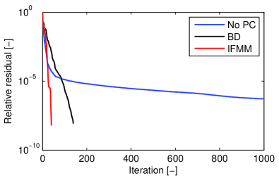 (b)

Figure 2: (a) Relative residual as a function of the iteration step and (b) total CPU time obtained without a preconditioner (No PC), a block-diagonal preconditioner (BD), and the IFMM as the preconditioner (IFMM) for a shear flow problem with $M=22$ pores and $N=10\,\mathrm{k}$ unknowns. The number of GMRES iterations is restricted to 1000.

Table 1: Overview of the results for various preconditioning strategies for a shear flow problem with $M=22$ pores and $N=10\,\mathrm{k}$ unknowns. The number of GMRES iterations is restricted to 1000.

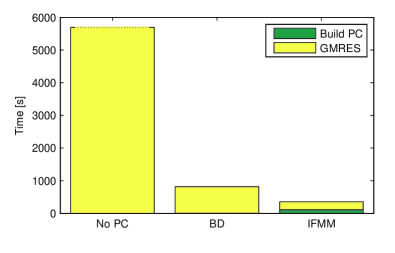
	# iterations	Total CPU time [s]	$\|\mathbf{P}^{-1}\mathbf{f}-\mathbf{P}^{-1}\mathbf{A}\widehat{\bm{\sigma}}\|_{2}/\|\mathbf{P}^{-1}\mathbf{f}\|_{2}$	$\|\mathbf{f}-\mathbf{A}\widehat{\bm{\sigma}}\|_{2}/\|\mathbf{f}\|_{2}$
		(Build PC + GMRES)
No PC	1000	$5.69\times 10^{3}$ (0 + $5.69\times 10^{3}$)	$5.16\times 10^{-7}$	$5.16\times 10^{-7}$
BD	139	$8.16\times 10^{2}$ ($2.51\times 10^{0}$ + $8.13\times 10^{2}$)	$8.87\times 10^{-9}$	$8.89\times 10^{-9}$
IFMM	40	$3.52\times 10^{2}$ ($1.11\times 10^{2}$ + $2.41\times 10^{2}$)	$6.54\times 10^{-9}$	$6.54\times 10^{-9}$

The density vector $\bm{\sigma}$ and the absolute value of the residual vector $\mathbf{r}=\mathbf{f}-\mathbf{A}\bm{\sigma}$ are shown in Figure 3(a) and Figure 3(b) for the block-diagonal and IFMM preconditioner, respectively. Because of the boundary condition chosen, the density function is exactly zero on the boundaries of the pores (the first $2\times 128\times 22=5632$ degrees of freedom). Generally speaking, the residual is somewhat smaller for the IFMM than for the block-diagonal preconditioner.

(a)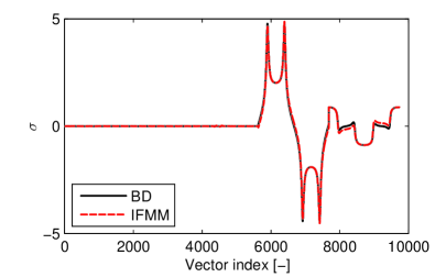 (b)

Figure 3: (a) Density vector $\bm{\sigma}$ and (b) absolute value of the residual vector $\mathbf{r}=\mathbf{f}-\mathbf{A}\bm{\sigma}$, obtained with a block-diagonal preconditioner (BD), and the IFMM as preconditioner (IFMM), for a shear flow problem with $M=22$ pores and $N=10\,\mathrm{k}$ unknowns.

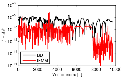
The accuracy of the solutions is further assessed with the logarithm of the relative error in the magnitude of the velocity field

$$\bm{\varepsilon}(\mathbf{x})=\frac{\big{|}\|\mathbf{u}(\mathbf{x})\|-\|\mathbf{u}_{\mathrm{ref}}(\mathbf{x})\|\big{|}}{\|\mathbf{u}_{\mathrm{ref}}(\mathbf{x})\|}.$$

We plot the error with both the block-diagonal and the IFMM preconditioner in Figure 4. We see that the errors are small in both cases, although the IFMM leads to errors that are almost two full orders of magnitude smaller. The largest errors are observed in both cases along the line $y=0$ where the magnitude of the reference velocity field is exactly zero.

(a) 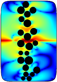     (b) 

Figure 4: Logarithm of the relative velocity magnitude error $\bm{\varepsilon}(\mathbf{x})=\big{|}\|\mathbf{u}(\mathbf{x})\|-\|\mathbf{u}_{\mathrm{ref}}(\mathbf{x})\|\big{|}/\|\mathbf{u}_{\mathrm{ref}}(\mathbf{x})\|$ obtained with (a) the block-diagonal preconditioner and (b) the IFMM preconditioner, for a shear flow problem with $M=22$ pores and $N=10\,\mathrm{k}$ unknowns.

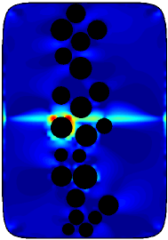
4.1.2 $M=226$ pores

We now consider the geometry in Figure 6 which contains 226 pores. We still discretize each pore with $N_{\mathrm{int}}=128$ points, but the longer outer wall is discretized with $N_{\mathrm{ext}}=4096$ points, leading to a problem with $66\,\mathrm{k}$ unknowns. The block-diagonal preconditioner and the IFMM are used as preconditioners in GMRES. The number of Chebyshev nodes in the IFMM is first chosen as $n=10$, but $n=15$ is also investigated since the matrix is expected to be more ill-conditioned than in the previous example. Results for unpreconditioned GMRES are not reported since it requires over 1000 iterations.

Figure 5(a) shows the relative residual as a function of the number of GMRES iterations for all the preconditioning strategies. GMRES with a block-diagonal preconditioner requires 785 iterations to converge to the specified residual, which is significantly larger than the number required in the previous example (see Figure 2(a)). This demonstrates that a preconditioner that does not include inter-dependence between pores is too simplistic to be effective for this complex geometry. Application of the IFMM, on the other hand, results in a faster convergence of the residual. The IFMM preconditioner with $n=10$ requires 501 iterations, and with $n=15$ requires 277 iterations.

The computation time of each preconditioning approach is depicted in Figure 5(b). The most expensive preconditioner to construct is the IFMM with $n=15$. However, because of the reduction in the number of GMRES iterations, this preconditioner leads to the smallest overall computation time and is more than twice as fast as the block-diagonal preconditioner.

(a)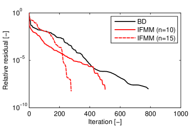 (b)

Figure 5: (a) Relative residual as a function of the iteration step and (b) total CPU time obtained with a block-diagonal preconditioner (BD), and the IFMM as preconditioner (IFMM), for a shear flow problem with $M=226$ pores and $N=66\,\mathrm{k}$ unknowns.

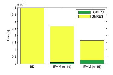
Apart from achieving a speedup, application of the IFMM also leads to a more accurate solution than the block-diagonal preconditioner. This is highlighted in the two last columns of Table 2: although the preconditioned residual $\|\mathbf{P}^{-1}\mathbf{f}-\mathbf{P}^{-1}\mathbf{A}\widehat{\bm{\sigma}}\|_{2}/\|\mathbf{P}^{-1}\mathbf{f}\|_{2}$ has reached the desired tolerance for the block-diagonal preconditioner, the actual residual $\|\mathbf{f}-\mathbf{A}\widehat{\bm{\sigma}}\|_{2}/\|\mathbf{f}\|_{2}$ is still several orders of magnitude larger.

Table 2: Overview of the results for various preconditioning strategies for a shear flow problem with $M=226$ pores and $N=66\,\mathrm{k}$ unknowns.

	# iterations	Total CPU time [s]	$\|\mathbf{P}^{-1}\mathbf{f}-\mathbf{P}^{-1}\mathbf{A}\widehat{\bm{\sigma}}\|_{2}/\|\mathbf{P}^{-1}\mathbf{f}\|_{2}$	$\|\mathbf{f}-\mathbf{A}\widehat{\bm{\sigma}}\|_{2}/\|\mathbf{f}\|_{2}$
		(Build PC + GMRES)
BD	785	$3.99\times 10^{4}$ ($1.78\times 10^{1}$ + $3.99\times 10^{4}$)	$1.00\times 10^{-8}$	$3.67\times 10^{-2}$
IFMM ($n=10$)	501	$2.68\times 10^{4}$ ($8.93\times 10^{2}$ + $2.59\times 10^{4}$)	$8.94\times 10^{-9}$	$8.94\times 10^{-9}$
IFMM ($n=15$)	277	$1.65\times 10^{4}$ ($2.34\times 10^{3}$ + $1.42\times 10^{4}$)	$5.94\times 10^{-9}$	$5.94\times 10^{-9}$

The accuracy of the solution is further assessed in Figure 6, showing the logarithm of the relative velocity magnitude error $\bm{\varepsilon}(\mathbf{x})$. The largest errors appear once again along the line $y=0$. Furthermore, the errors obtained with the IFMM are almost four orders of magnitude smaller than with the block-diagonal preconditioner. The results presented in Figure 5 and 6 clearly demonstrate the efficiency and accuracy of the IFMM for the challenging problem under concern.

(a)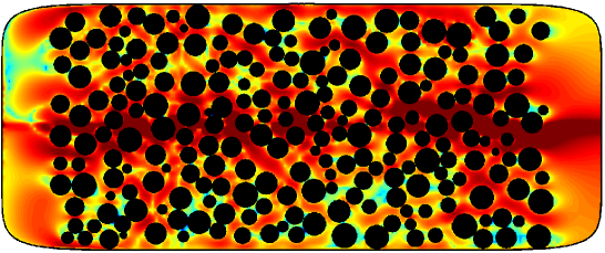 

(b)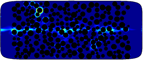 

Figure 6: Logarithm of the relative velocity magnitude error $\bm{\varepsilon}(\mathbf{x})=\big{|}\|\mathbf{u}(\mathbf{x})\|-\|\mathbf{u}_{\mathrm{ref}}(\mathbf{x})\|\big{|}/\|\mathbf{u}_{\mathrm{ref}}(\mathbf{x})\|$ obtained using (a) the block-diagonal preconditioner and (b) the IFMM preconditioner, for a shear flow problem with $M=226$ pores and $N=66\,\mathrm{k}$ unknowns.

4.1.3 $M=826$ pores

Finally, the full geometry with 826 pores depicted in Figure 1 is considered. We discretize each pore with $N_{\mathrm{int}}=128$ points and the outer boundary with $N_{\mathrm{ext}}=16384$ points, leading to a problem with $244\,\mathrm{k}$ unknowns. The number of Chebyshev nodes in the IFMM is chosen as $n=15$, while the maximum number of GMRES iterations is increased to 2000.

Table 3 indicates that the block-diagonal preconditioner does not reach convergence within 2000 iterations, and that the actual residual remains very large. On the other hand, convergence is obtained after 1489 iterations with the IFMM (with a small actual residual), confirming its effectiveness even for large problems with a very complicated geometry. Figure 7 depicts the logarithm of the relative velocity magnitude error $\bm{\varepsilon}(\mathbf{x})$, as obtained with the IFMM preconditioner. The errors are larger than in the previous test cases (compare with Figure 4(b) and Figure 6(b)), but are still reasonably small.

Table 3: Overview of the results for various preconditioning strategies for a shear flow problem with $M=826$ pores and $N=244\,\mathrm{k}$ unknowns. The number of GMRES iterations is restricted to 2000.

	# iterations	Total CPU time [s]	$\|\mathbf{P}^{-1}\mathbf{f}-\mathbf{P}^{-1}\mathbf{A}\widehat{\bm{\sigma}}\|_{2}/\|\mathbf{P}^{-1}\mathbf{f}\|_{2}$	$\|\mathbf{f}-\mathbf{A}\widehat{\bm{\sigma}}\|_{2}/\|\mathbf{f}\|_{2}$
		(Build PC + GMRES)
BD	2000	$3.04\times 10^{5}$ ($3.57\times 10^{2}$ + $3.04\times 10^{5}$)	$7.44\times 10^{-6}$	$1.82\times 10^{-1}$
IFMM ($n=15$)	1489	$2.70\times 10^{5}$ ($8.83\times 10^{3}$ + $2.61\times 10^{5}$)	$9.98\times 10^{-9}$	$1.15\times 10^{-6}$

Figure 7: Logarithm of the relative velocity magnitude error $\bm{\varepsilon}(\mathbf{x})=\big{|}\|\mathbf{u}(\mathbf{x})\|-\|\mathbf{u}_{\mathrm{ref}}(\mathbf{x})\|\big{|}/\|\mathbf{u}_{\mathrm{ref}}(\mathbf{x})\|$ obtained using the IFMM preconditioner, for a shear flow problem with $M=826$ pores and $N=244\,\mathrm{k}$ unknowns.

4.2 A linear combination of Stokeslets and rotlets

The examples considered in Subsection missing 4.1 are repeated with the same number of discretization points ($N_{\mathrm{int}}=128$ points per pore and $N_{\mathrm{ext}}=2048,4096,16384$ for the outer boundary), but with a boundary condition that results in a non-zero density vector $\bm{\sigma}$ on the boundaries of the inner pores. The boundary condition is given by a linear combination of Stokeslets and rotlets

$$\mathbf{f}(\mathbf{x})=\sum_{k=0}^{M}\left(-\log\|\mathbf{x}-\mathbf{c}_{k}\|\mathbf{I}+\frac{\left(\mathbf{x}-\mathbf{c}_{k}\right)\otimes\left(\mathbf{x}-\mathbf{c}_{k}\right)}{\|\mathbf{x}-\mathbf{c}_{k}\|^{2}}\right)\bm{\lambda}_{k}+\sum_{k=0}^{M}\frac{\left(\mathbf{x}-\mathbf{c}_{k}\right)^{\perp}}{\|\mathbf{x}-\mathbf{c}_{k}\|^{2}}\mu_{k},\quad\mathbf{x}\in\Gamma$$ (15)

where $\mathbf{c}_{0}$ is an arbitrary point located outside the domain $\Omega_{0}$ and $\mathbf{c}_{k}$ ($k=1\ldots M$) are arbitrary points inside each of the pores $\Omega_{k}$. The vectors $\bm{\lambda}_{k}$ and scalars $\mu_{k}$ are randomly chosen, and $(x,y)^{\perp}=(y,-x)$. The exact velocity field $\mathbf{u}_{\mathrm{ref}}(\mathbf{x})$ at any point $\mathbf{x}\in\Omega$ is given by Eq. (missing) 15 as well.

4.2.1 $M=22$ pores

We again consider the first 22 pores. The GMRES convergence results are very similar to the shear flow example: no convergence is achieved in 1000 iterations without preconditioning, while 143 and only 54 iterations are needed with the block-diagonal and the IFMM preconditioners, respectively. The results are summarized in Table 4. We see that the IFMM preconditioner is nearly twice as fast as the block-diagonal preconditioner.

Table 4: Overview of the results for various preconditioning strategies for a Stokeslets/rotlets flow problem with $M=22$ pores and $N=10\,\mathrm{k}$ unknowns. The number of GMRES iterations is restricted to 1000.

	# iterations	Total CPU time [s]	$\|\mathbf{P}^{-1}\mathbf{f}-\mathbf{P}^{-1}\mathbf{A}\widehat{\bm{\sigma}}\|_{2}/\|\mathbf{P}^{-1}\mathbf{f}\|_{2}$	$\|\mathbf{f}-\mathbf{A}\widehat{\bm{\sigma}}\|_{2}/\|\mathbf{f}\|_{2}$
		(Build PC + GMRES)
No PC	1000	$5.65\times 10^{3}$ (0 + $5.65\times 10^{3}$)	$2.39\times 10^{-5}$	$2.39\times 10^{-5}$
BD	143	$8.39\times 10^{2}$ ($2.44\times 10^{0}$ + $8.36\times 10^{2}$)	$8.61\times 10^{-9}$	$8.65\times 10^{-9}$
IFMM	55	$4.37\times 10^{2}$ ($1.20\times 10^{2}$ + $3.18\times 10^{2}$)	$3.79\times 10^{-9}$	$3.79\times 10^{-9}$

With this boundary condition, the density vector $\bm{\sigma}$ is non-zero on the boundary of each inner pore (Figure 8(a)). A good correspondence between the results of both preconditioners is found. Figure 8(b) shows the logarithm of the relative velocity magnitude error $\bm{\varepsilon}(\mathbf{x})$ obtained with the IFMM. As in the shear flow example, about six digits of accuracy is achieved.

(a)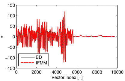    (b)

Figure 8: (a) Density vector $\bm{\sigma}$ obtained with a block-diagonal preconditioner (BD) and the IFMM as preconditioner (IFMM), and (b) logarithm of the relative velocity magnitude error $\bm{\varepsilon}(\mathbf{x})=\big{|}\|\mathbf{u}(\mathbf{x})\|-\|\mathbf{u}_{\mathrm{ref}}(\mathbf{x})\|\big{|}/\|\mathbf{u}_{\mathrm{ref}}(\mathbf{x})\|$ obtained with the IFMM preconditioner, for a linear combination of Stokeslets and rotlets with $M=22$ pores and $N=10\,\mathrm{k}$ unknowns.

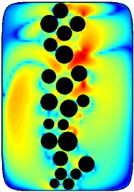
4.2.2 $M=226$ pores

We next increase the problem size to the first 226 pores and summarize the results in Table 5. GMRES with the block-diagonal preconditioner needs over 700 iterations to converge, while application of the IFMM reduces this number to 506 for $n=10$ and 258 for $n=15$. As we saw for the shear boundary condition, using $n=15$ Chebyshev nodes results in the smallest overall computation time, and this is almost 2.5 times faster than the block-diagonal preconditioner.

Table 5: Overview of the results for various preconditioning strategies for a Stokeslets/rotlets flow problem with $M=226$ pores and $N=66\,\mathrm{k}$ unknowns.

	# iterations	Total CPU time [s]	$\|\mathbf{P}^{-1}\mathbf{f}-\mathbf{P}^{-1}\mathbf{A}\widehat{\bm{\sigma}}\|_{2}/\|\mathbf{P}^{-1}\mathbf{f}\|_{2}$	$\|\mathbf{f}-\mathbf{A}\widehat{\bm{\sigma}}\|_{2}/\|\mathbf{f}\|_{2}$
		(Build PC + GMRES)
BD	715	$3.63\times 10^{4}$ ($1.81\times 10^{1}$ + $3.63\times 10^{4}$)	$9.94\times 10^{-9}$	$6.07\times 10^{-3}$
IFMM ($n=10$)	506	$2.68\times 10^{4}$ ($8.94\times 10^{2}$ + $2.59\times 10^{4}$)	$8.33\times 10^{-9}$	$8.33\times 10^{-9}$
IFMM ($n=15$)	258	$1.57\times 10^{4}$ ($2.35\times 10^{3}$ + $1.33\times 10^{4}$)	$7.33\times 10^{-9}$	$7.33\times 10^{-9}$

Similar to the shear flow example, there is a large discrepancy between the preconditioned and the actual residual for the block-diagonal preconditioner, while this is not the case for the IFMM (see Table 5). The errors inside the domain are consequently several orders of magnitude smaller when using the IFMM preconditioner as is illustrated in Figure 9.

(a)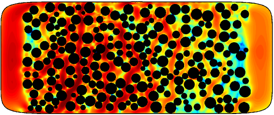 

(b)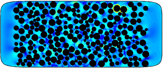 

Figure 9: Logarithm of the relative velocity magnitude error $\bm{\varepsilon}(\mathbf{x})=\big{|}\|\mathbf{u}(\mathbf{x})\|-\|\mathbf{u}_{\mathrm{ref}}(\mathbf{x})\|\big{|}/\|\mathbf{u}_{\mathrm{ref}}(\mathbf{x})\|$ obtained using (a) the block-diagonal preconditioner and (b) the IFMM preconditioner, for a Stokeslets/rotlets flow problem with $M=226$ pores and $N=66\,\mathrm{k}$ unknowns.

4.2.3 $M=826$ pores

Finally, all $826$ pores are considered. Table 6 indicates that no convergence is achieved with the block-diagonal preconditioner (even after 2000 iterations), while 1283 iterations are needed with the IFMM. Figure 10 confirms the accuracy of the solution obtained with the IFMM, although some localized spots with larger errors are observed.

Table 6: Overview of the results for various preconditioning strategies for a Stokeslets/rotlets flow problem with $M=826$ pores and $N=244\,\mathrm{k}$ unknowns. The number of GMRES iterations is restricted to 2000.

	# iterations	Total CPU time [s]	$\|\mathbf{P}^{-1}\mathbf{f}-\mathbf{P}^{-1}\mathbf{A}\widehat{\bm{\sigma}}\|_{2}/\|\mathbf{P}^{-1}\mathbf{f}\|_{2}$	$\|\mathbf{f}-\mathbf{A}\widehat{\bm{\sigma}}\|_{2}/\|\mathbf{f}\|_{2}$
		(Build PC + GMRES)
BD	2000	$3.04\times 10^{5}$ ($3.61\times 10^{2}$ + $3.04\times 10^{5}$)	$1.12\times 10^{-7}$	$7.23\times 10^{-2}$
IFMM ($n=15$)	1283	$2.24\times 10^{5}$ ($8.82\times 10^{3}$ + $2.16\times 10^{5}$)	$1.00\times 10^{-8}$	$1.34\times 10^{-7}$

Figure 10: Logarithm of the relative velocity magnitude error $\bm{\varepsilon}(\mathbf{x})=\big{|}\|\mathbf{u}(\mathbf{x})\|-\|\mathbf{u}_{\mathrm{ref}}(\mathbf{x})\|\big{|}/\|\mathbf{u}_{\mathrm{ref}}(\mathbf{x})\|$ obtained using the IFMM preconditioner, for a Stokeslets/rotlets flow problem with $M=826$ pores and $N=244\,\mathrm{k}$ unknowns.

4.3 Pipe flow

This final section considers the more physical boundary conditions defined in Eq. (missing) 4 and illustrated in Figure 1. The velocity is parabolic at the intake and outtake of the outer boundary $\Gamma_{0}$, and zero on each pore. The same number of discretization points as in Subsection missing 4.1 and 4.2 is used.

4.3.1 $M=22$ pores

Figure 11(a) shows the relative residual as a function of the number of GMRES iterations for the case involving 22 pores. The convergence behavior of the preconditioners is similar to the previous two examples. However, without preconditioning, the convergence is notably slower than before. The results are summarized in Table 7. The density vector $\bm{\sigma}$ obtained with the block-diagonal and IFMM preconditioners is depicted in Figure 11(b), illustrating a good match between both approaches.

(a)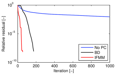 (b)

Figure 11: (a) Relative residual as a function of the iteration step and (b) density vector $\bm{\sigma}$, obtained without preconditioner (No PC), a block-diagonal preconditioner (BD), and the IFMM as preconditioner (IFMM) for a pipe flow problem with $M=22$ pores and $N=10\,\mathrm{k}$ unknowns.

Table 7: Overview of the results for various preconditioning strategies, for a pipe flow problem with $M=22$ pores and $N=10\,\mathrm{k}$ unknowns. The number of GMRES iterations is restricted to 1000.

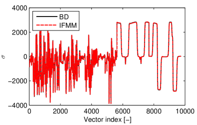
	# iterations	Total CPU time [s]	$\|\mathbf{P}^{-1}\mathbf{f}-\mathbf{P}^{-1}\mathbf{A}\widehat{\bm{\sigma}}\|_{2}/\|\mathbf{P}^{-1}\mathbf{f}\|_{2}$	$\|\mathbf{f}-\mathbf{A}\widehat{\bm{\sigma}}\|_{2}/\|\mathbf{f}\|_{2}$
		(Build PC + GMRES)
No PC	1000	$5.66\times 10^{3}$ (0 + $5.66\times 10^{3}$)	$8.81\times 10^{-3}$	$8.81\times 10^{-3}$
BD	173	$3.61\times 10^{2}$ ($2.44\times 10^{0}$ + $3.59\times 10^{2}$)	$8.95\times 10^{-9}$	$8.98\times 10^{-9}$
IFMM	54	$9.80\times 10^{1}$ ($1.72\times 10^{1}$ + $8.08\times 10^{1}$)	$7.07\times 10^{-9}$	$7.07\times 10^{-9}$

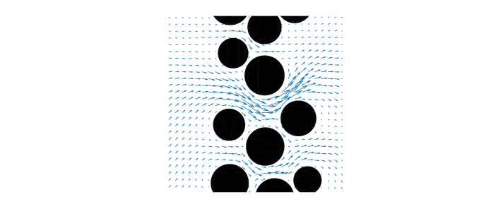
Figure 12 shows a quiver plot of the velocity field $\mathbf{u}(\mathbf{x})$ obtained with the block-diagonal and the IFMM preconditioner. The parabolic velocity profile imposed on the left side of the outer boundary is strongly affected by the presence of the pores, and large velocities are observed in the areas with the largest gaps between the pores.

Figure 12: Quiver plot of the velocity field $\mathbf{u}(\mathbf{x})$ obtained when using the IFMM preconditioner for a pipe flow problem with $M=22$ pores and $N=10\,\mathrm{k}$ unknowns. The velocity field is plotted in a small window in the middle of the porous region.

4.3.2 $M=226$ pores

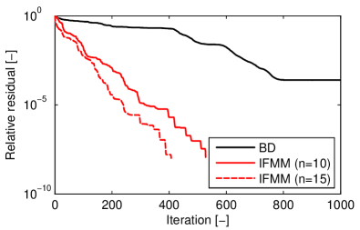
For all the examples considered so far, the block-diagonal preconditioner did not perform that badly; application of the IFMM has only lead to rather moderate speedups (up to a factor of 2.5). The pipe flow problem involving 226 pores turns out to be much harder for the block-diagonal preconditioner, however, as is indicated in Figure 13 and Table 8. Block-diagonal preconditioned GMRES is unable to converge within 1000 iterations and the residual is still more than four orders of magnitude above the prescribed tolerance of $10^{-8}$. Application of the IFMM, on the other hand, guarantees converge in 528 iterations for $n=10$ and slightly more than 400 iterations for $n=15$, hence confirming the effectiveness of the IFMM.

Figure 13: Relative residual as a function of the iteration step for a block-diagonal preconditioner (BD) and the IFMM preconditioner (IFMM) for a pipe flow with $M=226$ pores and $N=66\,\mathrm{k}$ unknowns. The number of GMRES iterations is restricted to 1000.

Table 8: Overview of the results for various preconditioning strategies for a pipe flow problem with $M=226$ pores and $N=66\,\mathrm{k}$ unknowns. The number of GMRES iterations is restricted to 1000.

	# iterations	Total CPU time [s]	$\|\mathbf{P}^{-1}\mathbf{f}-\mathbf{P}^{-1}\mathbf{A}\widehat{\bm{\sigma}}\|_{2}/\|\mathbf{P}^{-1}\mathbf{f}\|_{2}$	$\|\mathbf{f}-\mathbf{A}\widehat{\bm{\sigma}}\|_{2}/\|\mathbf{f}\|_{2}$
		(Build PC + GMRES)
BD	1000	$4.42\times 10^{4}$ ($1.81\times 10^{1}$ + $4.42\times 10^{4}$)	$2.45\times 10^{-4}$	$9.31\times 10^{-1}$
IFMM ($n=10$)	528	$1.30\times 10^{4}$ ($5.63\times 10^{2}$ + $1.24\times 10^{4}$)	$9.97\times 10^{-9}$	$4.64\times 10^{-6}$
IFMM ($n=15$)	407	$1.12\times 10^{4}$ ($1.81\times 10^{3}$ + $9.38\times 10^{3}$)	$9.94\times 10^{-9}$	$2.07\times 10^{-6}$

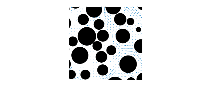
Figure 14 shows a quiver plot of the velocity field $\mathbf{u}(\mathbf{x})$ obtained with the IFMM preconditioner. Even though the governing equations are linear, the flow is very complex because of the geometry. With this velocity field, particle tracking can be performed, and this can be used to find structure within the flow [80]. However, this is only practical if the linear system Eq. (missing) 8 can be solved with a specified tolerance with a reasonable amount of computation time. With our proposed IFMM preconditioner, this is exactly the case.

Figure 14: Quiver plot of the velocity field $\mathbf{u}(\mathbf{x})$ obtained when using the IFMM preconditioner for a pipe flow problem with $M=226$ pores and $N=66\,\mathrm{k}$ unknowns. The velocity field is plotted in a small window in the middle of the porous region.

4.3.3 $M=826$ pores

Finally, the problem depicted in Figure 1 is solved. The block diagonal preconditioner is once more unable to reach convergence and the residual remains large after 2000 iterations, as is summarized in Table 9. GMRES would probably need a few more thousand iterations to converge with this preconditioner. The IFMM preconditioner needs 1645 iterations to converge, leading to a reasonably small actual residual.

Table 9: Overview of the results for various preconditioning strategies for a pipe flow problem with $M=826$ pores and $N=244\,\mathrm{k}$ unknowns. The number of GMRES iterations is restricted to 2000.

	# iterations	Total CPU time [s]	$\|\mathbf{P}^{-1}\mathbf{f}-\mathbf{P}^{-1}\mathbf{A}\widehat{\bm{\sigma}}\|_{2}/\|\mathbf{P}^{-1}\mathbf{f}\|_{2}$	$\|\mathbf{f}-\mathbf{A}\widehat{\bm{\sigma}}\|_{2}/\|\mathbf{f}\|_{2}$
		(Build PC + GMRES)
BD	2000	$3.04\times 10^{5}$ ($3.61\times 10^{2}$ + $3.04\times 10^{5}$)	$9.78\times 10^{-3}$	$9.48\times 10^{-1}$
IFMM ($n=15$)	1645	$2.96\times 10^{5}$ ($8.84\times 10^{3}$ + $2.87\times 10^{5}$)	$1.00\times 10^{-8}$	$2.67\times 10^{-5}$

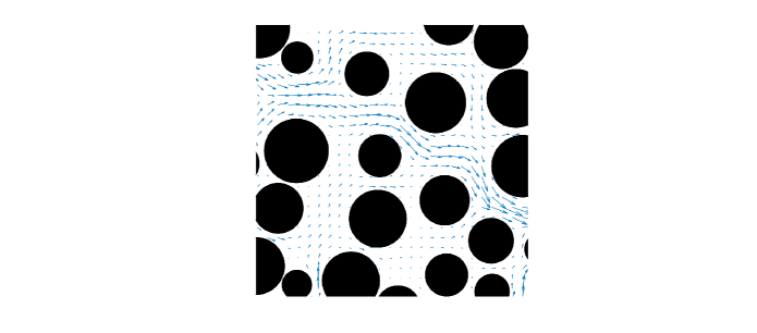
Figure 15 shows a quiver plot of the velocity field $\mathbf{u}(\mathbf{x})$ obtained with the IFMM preconditioner. A very complex flow is resolved in this case as well.

Figure 15: Quiver plot of the velocity field $\mathbf{u}(\mathbf{x})$ obtained when using the IFMM preconditioner for a pipe flow problem with $M=826$ pores and $N=244\,\mathrm{k}$ unknowns. The velocity field is plotted in a small window in the middle of the porous region.

5 Conclusions

Discretization of a first-kind boundary integral equation, representing a 2D incompressible Stokes flow in a porous medium, leads to a dense linear system of equations that is computationally expensive to solve. In particular, a large number of iterations is often required if an iterative Krylov methods such as GMRES is employed. In this paper, the IFMM has been presented as an efficient preconditioner that is capable of significantly reducing the number of iterations and the overall computation cost.

The IFMM is in essence an inexact fast direct solver for dense $\mathcal{H}^{2}$-matrices with a linear complexity. This complexity is achieved through two key ideas: the hierarchical low-rank structure of the matrix is exploited to represent the original system as an extended sparse system, and low-rank (re)compressions are applied to maintain the sparsity pattern of the latter throughout the Gaussian elimination. The solver has a tunable accuracy $\varepsilon$ allowing for a trade-off between a highly accurate direct solver and a low-accurate preconditioner.

Various numerical benchmarks have been carried out to validate the accuracy and to assess the efficacy of the IFMM as a preconditioner. It has been demonstrated that the IFMM preconditioner outperforms a block-diagonal preconditioner for several types of boundary conditions. This is especially the case for pipe flow problems involving many pores, which is relevant for various practical applications.

Finally, it is important to note that the current IFMM implementation is based on a uniform quadtree decomposition of the domain, which is far from optimal for the complex geometries considered in this paper. The use of an adaptive quadtree is expected to make the IFMM even more efficient.

References

- [1] Cueto-Felgueroso L, Juanes R. Nonlocal Interface Dynamics and Pattern Formation in Gravity-Driven Unsaturated Flow Through Porous Media. Physical Review Letters 2008; 101(24):244 504.
- [2] Kitamura K, Jiang F, Valocchi AJ, Chiyonobu S, Tsuji T, Christensen KT. The study of heterogeneous two-phase flow around small-scale heterogeneity in porous sandstone by measured elastic wave velocities and lattice Boltzmann method simulation. Journal of Geophysical Research: Solid Earth 2014; 119(10):7564–7577.
- [3] McDowell-Boyer LM, Hunt JR, Sitar N. Particle Transport Through Porous Media. Water Resources Research 1986; 22(13):1901–1921.
- [4] Vardoulakis I, Stavropoulou M, Papanastasiou P. Hydromechanical aspects of the sand production problem. Transport in porous media 1996; 22(2):225–244.
- [5] Wang CY. Fundamental Models for Fuel Cell Engineering. Chemical Reviews 2004; 104(10):4727–4766.
- [6] Lecoanet HF, Bottero JY, Wiesner MR. Laboratory Assessment of the Mobility of Nanomaterials in Porous Media. Environmental Science & Technology 2004; 38(19):5164–5169.
- [7] Wu D, Liu H, Xie M, Liu H, Sun W. Experimental investigation on low velocity filtration combustion in porous packed bed using gaseous and liquid fuels. Experimental Thermal and Fluid Science 2012; 36:169–177.
- [8] Wu YS, Ye M, Sudicky EA. Fracture-Flow-Enhanced Matrix Diffusion in Solute Transport Through Fractured Porous Media. Transport in Porous Media 2010; 81(1):21–34.
- [9] Borgne TL, Dentz M, Villermaux E. Stretching, Coalescence, and Mixing in Porous Media. Physical Review Letters 2013; 110(20):204 501.
- [10] Hidalgo JJ, Fe J, Cueto-Felgueroso L, Juanes R. Scaling of Convective Mixing in Porous Media. Physical Review Letters 2012; 109(26):264 503.
- [11] Berkowitz B, Scher H, Silliman SE. Anomalous transport in laboratory-scale, heterogeneous porous media. Water Resources Research 2000; 36(1):149–158.
- [12] Sun H, Chen W, Chen Y. Variable-order fractional differential operators in anomalous diffusion modeling. Physica A: Statistical Mechanics and its Applications 2009; 388(21):4586–4592.
- [13] Haggerty R, McKenna SA, Meigs LC. On the late-time behavior of tracer test breakthrough curves. Water Resources Research 2000; 36(12):3467–3479.
- [14] Kazemifar F, Blois G, Kyritsis DC, Christensen KT. Quantifying the flow dynamics of supercritical CO2–water displacement in a 2D porous micromodel using fluorescent microscopy and microscopic PIV. Advances in Water Resources 2015; .
- [15] Szulczewski ML, Hesse M, Juanes R. Carbon dioxide dissolution in structural and stratigraphic traps. Journal of Fluid Mechanics 2013; 736:287–315.
- [16] Icardi M, Boccardo G, Tempone R. On the predictivity of pore-scale simulations: Estimating uncertainties with multilevel Monte Carlo. Advances in Water Resources 2016; .
- [17] Meyer DW, Tchelepi HA, Jenny P. A fast simulation method for uncertainty quantification of subsurface flow and transport. Water Resources Research 2013; 49(5):2359–2379.
- [18] Dentz M, Borgne TL, Englert A, Bijeljic B. Mixing, spreading and reaction in heterogeneous media: A brief review. Journal of Contaminant Hydrology 2011; 120:1–17.
- [19] Tél T, de Moura A, Grebogi C, Károlyi G. Chemical and biological activity in open flows: A dynamical system approach. Physics Reports 2005; 413(2):91–196.
- [20] Lebon L, Oger L, Leblond J, Hulin JP, Martys NS, Schwartz LM. Pulsed gradient NMR measurements and numerical simulation of flow velocity distribution in sphere packings. Physics of Fluids 1996; 8(2):293–301.
- [21] Icardi M, Boccardo G, Marchisio DL, Tosco T, Sethi R. Pore-scale simulation of fluid flow and solute dispersion in three-dimensional porous media. Physical Review E 2014; 90(1):013 032.
- [22] Jr JSA, Almeida MP, Filho JM, Havlin S, Suki B, Stanley HE. Fluid Flow through Porous Media: The Role of Stagnant Zones. Physical Review Letters 1997; 79(20):3901.
- [23] Blunt MJ, Bijeljic B, Dong H, Gharbi O, Iglauer S, Mostaghimi P, Paluszny A, Pentland C. Pore-scale imaging and modelling. Advances in Water Resources 2013; 51:197–216.
- [24] Manz B, Gladden LF, Warren PB. Flow and Dispersion in Porous Media: Lattice-Boltzmann and NMR Studies. AIChE journal 1999; 45(9):1845–1854.
- [25] de Anna P, Borgne TL, Dentz M, Tartakovsky AM, Bolster D, Davy P. Flow Intermittency, Dispersion, and Correlated Continuous Time Random Walks in Porous Media. Physical Review Letters 2013; 110(18):184 502.
- [26] Liu PL, Cheng AHD, Liggett JA, Lee JH. Boundary Integral Equation Solutions to Moving Interface Between Two Fluids in Porous Media. Water Resources Research 1981; 17(5):1445–1452.
- [27] Lough MF, Lee SH, Kamath J. An Efficient Boundary Integral Formulation for Flow Through Fractured Porous Media. Journal of Computational Physics 1998; 143(2):462–483.
- [28] Malholtra D, Gholami A, Biros G. A volume integral equation Stokes solver for problems with variable coefficients. Proceedings of the International Conference for High Performance Computing, Networking, Storage and Analysis, IEEE Press, 2014; 92–102.
- [29] Campbell SL, Ipsen ICF, Kelley CT, Meyer CD, Xue ZQ. Convergence estimates for solution of integral equations with GMRES. Journal of Integral Equations and Applications 1996; 8(1):19–34.
- [30] Greengard L, Rokhlin V. A Fast Algorithm for Particle Simulations. Journal of Computational Physics 1987; 73:325–348.
- [31] Ying L, Biros G, Zorin D. A kernel-independent adaptive fast multipole algorithm in two and three dimensions. Journal of Computational Physics 2004; 194(2):591–626.
- [32] Darden T, York D, Pedersen L. Particle mesh Ewald: An method for Ewald sums in large systems. The Journal of Chemical Physics 1993; 98(12):10 089–10 092.
- [33] Barnes J, Hut P. A hierarchical force-calculation algorithm. Nature Publishing Group 1986; 324:446–449.
- [34] Quaife B, Biros G. On preconditioners for the Laplace double-layer potential in 2D. Numerical Linear Algebra with Applications 2015; 22:101–122.
- [35] Colton D, Kress R. Inverse Acoustic and Electromagnetic Scattering Theory, vol. 93. Springer Science & Business Media, 2012.
- [36] Hsiao GC, Wendland WL. Boundary Integral Equations. Springer: Berlin, 2008.
- [37] Heuer N, Stephan EP, Tran T. Multilevel additive Schwarz method for the h-p version of the Galerkin boundary element method. Mathematics of Computation of the American Mathematical Society 1998; 67(222):501–518.
- [38] Maischak M, Stephan EP, Tran T. Multiplicative Schwarz algorithms for the Galerkin boundary element method. SIAM Journal on Numerical Analysis 2000; 38(4):1243–1268.
- [39] Funken SA, Stephan EP. The BPX preconditioner for the single layer potential operator. Applicable Analysis 1997; 67(3-4):327–340.
- [40] Chen K. An Analysis of Sparse Approximate Inverse Preconditioners for Boundary Integral Equations. SIAM Journal on Matrix Analysis and Applications 2000; 22(4):1058–1078.
- [41] Grama A, Kumar V, Sameh A. Parallel Hierarchical Solvers and Preconditioners for Boundary Element Methods. SIAM Journal on Scientific Computing 1997; 20(1):337–358.
- [42] Bebendorf M. Hierarchical LU decomposition-based preconditioners for BEM. Computing 2005; 74(3):225–247.
- [43] Nabors K, Korsmeyer FT, Leighton FT, White JK. Preconditioned, adaptive, multipole-accelerated iterative methods for three-dimensional first-kind integral equations of potential theory. SIAM Journal on Scientific and Statistical Computing 1994; 15:713–735.
- [44] Vavasis SA. Preconditioning for boundary integral equations. SIAM Journal on Matrix Analysis and Applications 1992; 13(3):905–925.
- [45] Steinbach O, Wendland W. The construction of some efficient preconditioners in the boundary element method. Advances in Computational Mathematics 1998; 9:191–216.
- [46] Bramble JH, Leyk Z, Pasciak JE. The Analysis of Multigrid Algorithms for Pseudodifferential Operators of Order Minus One. Mathematics of Computation October 208; 63(208):461–478.
- [47] Hsiao GC, Xu L, Zhang S. Solving Negative Order Equations by the Multigrid Method Via Variable Substitution. Journal of Scientific Computing 2014; 59(2):371–385.
- [48] Langer U, Pusch D, Reitzinger S. Efficient preconditioners for boundary element matrices based on grey-box algebraic multigrid methods. International Journal for Numerical Methods in Engineering 2003; 58(13):1937–1953.
- [49] Of G. An efficient algebraic multigrid preconditioner for a fast multipole boundary element method. Computing 2008; 82:139–155.
- [50] Langer U, Pusch D. Data-sparse algebraic multigrid methods for large scale boundary element equations. Applied Numerical Mathematics 2005; 54(3):406–424.
- [51] Aminfar A, Ambikasaran S, Darve E. A Fast Block Low-Rank Dense Solver with Applications to Finite-Element Matrices. arXiv 2014; :1403.5337.
- [52] Chandrasekaran M S Gu, Pals T. A fast ULV decomposition solver for hierarchically semi-separable representations. SIAM Journal on Matrix Analysis and Applications 2006; 28(3):603–622.
- [53] Sheng Z, Dewilde P, Chandrasekaran S. Algorithms to Solve Hierarchically Semi-separable Systems. System Theory, the Schur Algorithm and Multidimensional Analysis, Operator Theory: Advances and Applications, vol. 176, Alpay D, Vinnikov V (eds.). Birkhäuser Basel, 2007; 255–294.
- [54] Bebendorf M. Hierarchical Matrices: A Means to Efficiently Solve Elliptic Boundary Value Problems. 1st edn., Springer Publishing Company, 2008.
- [55] Börm S. Data-sparse approximation of non-local operators by -matrices. Linear Algebra and its Applications 2007; 422(2):380–403.
- [56] Hackbusch W, Börm S. Data-sparse Approximation by Adaptive -Matrices. Computing 2002; 69(1):1–35.
- [57] Gillman A, Martinsson PG. An algorithm for constructing the solution operator to 2D elliptic boundary value problems in the absence of body loads. Advances in Computational Mathematics 2014; 40(4):773–796.
- [58] Kong W, Bremer J, Rokhlin V. An adaptive fast direct solver for boundary integral equations in two dimensions. Applied and Computational Harmonic Analysis 2011; 31(3):346–369.
- [59] Martinsson PG, Rokhlin V. A fast direct solver for boundary integral equations in two dimensions. Journal of Computational Physics 2005; 205(1):1–23.
- [60] Marple GR, Barnett A, Gillman A, Veerapaneni S. A fast algorithm for simulating multiphase flows through periodic geometries of arbitrary shape. arXiv 2015; 1510.05616.
- [61] Gillman A, Barnett A. A fast direct solver for quasi-periodic scattering problems. Journal of Computational Physics 2013; 248:309–322.
- [62] Gillman A, Barnett A, Martinsson PG. A spectrally accurate direction solution technique for frequency-domain scattering problems with variable media. BIT Numerical Mathematics 2014; 55(1):141–170.
- [63] Ambikasaran S, Darve E. The Inverse Fast Multipole Method. arxiv 2014; 1407.1572.
- [64] Coulier P, Pouransari H, Darve E. The inverse fast multipole method: using a fast approximate direct solver as a preconditioner for dense linear systems. arXiv 2015; :1508.01 835.
- [65] Power H. The completed double layer boundary integral equation method for two-dimensional Stokes flow. IMA Journal of Applied Mathematics 1993; 51(2):123–145.
- [66] Pozrikidis C. Boundary Integral and Singularity Methods for Linearized Viscous Flow. Cambridge University Press: New York, NY, USA, 1992.
- [67] Kapur S, Rokhlin V. High-Order Corrected Trapezoidal Quadrature Rules for Singular Functions. SIAM Journal on Numerical Analysis 1997; 34(4):1331–1356.
- [68] Alpert BK. Hybrid Gauss-Trapezoidal Quadrature Rules. SIAM Journal on Scientific Computing 1999; 20:1551–1584.
- [69] Barnett A, Wu B, Veerapaneni S. Spectrally-Accurate Quadratures for Evaluation of Layer Potentials Close to the Boundary for the 2D Stokes and Laplace Equations. arXiv 2014; 1410.2187.
- [70] Ying L, Biros G, Zorin D. A high-order 3D boundary integral equation solver for elliptic PDEs in smooth domains. Journal of Computational Physics 2006; 219(1):247–275.
- [71] Coulier P, Darve E. Efficient mesh deformation based on radial basis function interpolation by means of the inverse fast multipole method. Computer Methods in Applied Mechanics and Engineering 2016; .
- [72] Xia J, Chandrasekaran S, Gu M, Li X. Fast algorithms for hierarchically semiseparable matrices. Numerical Linear Algebra with Applications 2010; 17(6):953–976.
- [73] Xia J, Chandrasekaran S, Gu M, Li X. Superfast Multifrontal Method for Large Structured Linear Systems of Equations. SIAM Journal on Matrix Analysis and Applications 2010; 31(3):1382–1411.
- [74] Ambikasaran S, Darve E. An Fast Direct Solver for Partial Hierarchically Semi-Separable Matrices. Journal of Scientific Computing 2013; 57(3):477–501.
- [75] Corona E, Martinsson PG, Zorin D. A direct solver for integral equations on the plane. Applied and Computational Harmonic Analysis 2015; 38(2):284–317.
- [76] Lizé B. Fast Direct Solver for the Boundary Element Method in Electromagnetism and Acoustics: -Matrices. Parallelism and Industrial Applications. PhD Thesis, Université Paris 13 2014.
- [77] Saad Y, Schultz M. GMRES: A Generalized Minimal Residual Algorithm for Solving Nonsymmetric Linear Systems. SIAM Journal on Scientific and Statistical Computing 1986; 7:856–869.
- [78] Fong W, Darve E. The black-box fast multipole method. Journal of Computational Physics 2009; 228(23):8712–8725.
- [79] Hsiao GC, Kopp P, Wendland WL. A Galerkin Collocation Method for Some Integral Equations of the First Kind. Computing 1980; 25(2):89–130.
- [80] Haller G. Distinguished material surfaces and coherent structures in three-dimensional fluid flows. Physica D 2001; 149:248–277.