Robust recovery-type a posteriori error estimators for streamline upwind/Petrov Galerkin discretizations for singularly perturbed problems

Shaohong Du School of Mathematics and Statistics, Chongqing Jiaotong University, Chongqing 400074, China. E-mail: dushaohong@csrc.ac.cn, duzheyan.student@sina.com.cn. Research partially supported by the National Natural Science Foundation of China under grants 91430216, 11471031.    Runchang Lin Department of Mathematics and Physics, Texas A&M International University, Laredo, Texas 78041, USA. E-mail: rlin@tamiu.edu. Research partially supported by the US National Science Foundation grant 1217268 and by a University Research Grant of Texas A&M International University.    Zhimin Zhang Beijing Computational Science Research Center, Beijing 100193, China and Department of Mathematics, Wayne State University, Detroit, Michigan 48202, USA. E-mail: zmzhang@csrc.ac.cn, zzhang@math.wayne.edu. Research partially supported by the US National Science Foundation through grant DMS-1419040 and by the National Natural Science Foundation of China under grants 91430216, 11471031.
Abstract

In this paper, we investigate adaptive streamline upwind/Petrov Galerkin (SUPG) methods for singularly perturbed convection-diffusion-reaction equations in a new dual norm presented in [15]. The flux is recovered by either local averaging in conforming H(div)𝐻divH({\rm div}) spaces or weighted global L2superscript𝐿2L^{2} projection onto conforming H(div)𝐻divH({\rm div}) spaces. We further introduce a recovery stabilization procedure, and develop completely robust a posteriori error estimators with respect to the singular perturbation parameter ε𝜀\varepsilon. Numerical experiments are reported to support the theoretical results and to show that the estimated errors depend on the degrees of freedom uniformly in ε𝜀\varepsilon.

Keywords: singular perturbation, streamline upwind/Petrov Galerkin method, recovery-type a posteriori error estimator, robust.

2010 Mathematics Subject Classification. 65N15, 65N30, 65J15

1 Introduction

Let ΩΩ\Omega be a bounded polygonal or polyhedral domain in dsuperscript𝑑{\mathbb{R}}^{d} (d=2𝑑2d=2 or 333) with Lipschitz boundary Γ=ΓDΓNΓsubscriptΓ𝐷subscriptΓ𝑁\Gamma=\Gamma_{D}\cup\Gamma_{N}, where ΓDΓN=subscriptΓ𝐷subscriptΓ𝑁\Gamma_{D}\cap\Gamma_{N}=\emptyset. Consider the following stationary singularly perturbed convection-diffusion-reaction problem

{u:=εu+𝐚u+bu=finΩ,u=0onΓD,εu𝐧=gonΓN,casesassign𝑢𝜀𝑢𝐚𝑢𝑏𝑢𝑓inΩ𝑢0onsubscriptΓ𝐷𝜀𝑢𝐧𝑔onsubscriptΓ𝑁\left\{\begin{array}[]{rl}\mathcal{L}u:=-\varepsilon\triangle u+{\bf a}\cdot\nabla u+bu=f&\mbox{in}~{}\Omega,\\ u=0&\mbox{on}~{}\Gamma_{D},\\ \displaystyle\varepsilon\frac{\partial u}{\partial{\bf n}}=g&\mbox{on}~{}\Gamma_{N},\end{array}\right. (1.1)

where 0<ε10𝜀much-less-than10<\varepsilon\ll 1 is the singular perturbation parameter, 𝐚(W1,(Ω))d𝐚superscriptsuperscript𝑊1Ω𝑑{\bf a}\in(W^{1,\infty}(\Omega))^{d}, bL(Ω)𝑏superscript𝐿Ωb\in L^{\infty}(\Omega), fL2(Ω)𝑓superscript𝐿2Ωf\in L^{2}(\Omega), 𝐧𝐧{\bf n} is the outward unit normal vector to ΓΓ\Gamma, and equation (1.1) is scaled such that 𝐚L=𝒪(1)subscriptnorm𝐚superscript𝐿𝒪1||{\bf a}||_{L^{\infty}}=\mathcal{O}(1) and bL=𝒪(1)subscriptnorm𝑏superscript𝐿𝒪1||b||_{L^{\infty}}=\mathcal{O}(1). The Dirichlet boundary ΓDsubscriptΓ𝐷\Gamma_{D} has a positive (d1)𝑑1(d-1)-dimensional Lebesgue measure, which includes the inflow boundary {𝐱Ω:𝐚(𝐱)𝐧<0}conditional-set𝐱Ω𝐚𝐱𝐧0\{{\bf x}\in\partial\Omega:{\bf a}({\bf x})\cdot{\bf n}<0\}. Assume that there are two nonnegative constants β𝛽\beta and cbsubscript𝑐𝑏c_{b}, independent of ε𝜀\varepsilon, satisfying

b12𝐚βandbL(Ω)cbβ.formulae-sequence𝑏12𝐚𝛽andsubscriptnorm𝑏superscript𝐿Ωsubscript𝑐𝑏𝛽b-\frac{1}{2}\nabla\cdot{\bf a}\geq\beta\quad\text{and}\quad||b||_{L^{\infty}{(\Omega)}}\leq c_{b}\beta. (1.2)

Note that if β=0𝛽0\beta=0, then b0𝑏0b\equiv 0 and there is no reaction term in (1.1).

Adaptive finite element methods (FEMs) for numerical solutions of partial differential equations (PDEs) are very popular in scientific and engineering computations. A posteriori error estimation is an essential ingredient of adaptivity. Error estimators in literature can be categorized into three classes: residual based, gradient recovery based, and hierarchical bases based. Each approach has certain advantages.

Designing a robust a posteriori error estimator for singularly perturbed equations is challenging, because the estimators usually depend on the small diffusion parameter ε𝜀\varepsilon. This problem was first investigated by Verfürth [27], in which both upper and lower bounds for error estimator in an ε𝜀\varepsilon-weighted energy norm was proposed. It was shown that the estimator was robust when the local Péclet number is not very large. Generalization of this approach can be found in, e.g., [8, 19, 22, 24]. He considered also robust estimators in an ad hoc norm in [28]. In [25], Sangalli pointed out that the ad hoc norm may not be appropriate for problem (1.1), and proposed a residual-type a posteriori estimator for 1D convection-diffusion problem which is robust up to a logarithmic factor with respect to global Péclet number. Recently, John and Novo [18] proposed a robust a posteriori error estimator in the natural SUPG norm (used in the a priori analysis) under some hypotheses, which, however, may not be fulfilled in practise. In [2], a fully computable, guaranteed upper bounds are developed for the discretisation error in energy norm. Very recently, Tobiska and Verfürth [26] presented robust residual a priori error estimates for a wide range of stabilized FEMs.

For a posteriori error estimation of singularly perturbed problems, it is crucial to employ an appropriate norm, since the efficiency of a robust estimator depends fully on the norm. Du and Zhang [15] proposed a dual norm, which is induced by an ε𝜀\varepsilon-weighted energy norm and a related H1/2(Ω)superscript𝐻12ΩH^{1/2}(\Omega)-norm. A uniformly robust a posteriori estimator for the numerical error was obtained from the new norm. Both theoretical and numerical results showed that the estimator performs better than the existing ones in the literature.

It is well known that the a posteriori error estimators of the recovery type possess many appealing properties, including simplicity, university, and asymptotical exactness, which lead to their widespread adoption, especially in the engineering community (cf., e.g., [3, 4, 7, 11, 30, 31, 32, 33]). However, when applied to many problems of practical interest, such as interface singularities, discontinuities in the form of shock-like fronts, and of interior or boundary layers, they lose not only asymptotical exactness but also efficiency on relatively coarse meshes. They may overrefine regions where there are no error, and hence fail to reduce the global error (see [6, 20, 21]). To overcome this difficulty, Cai and Zhang [9] developed a global recovery approach for the interface problem. The flux is recovered in H(div)𝐻divH({\rm div}) conforming finite element (FE) spaces, such as the Raviart-Thomas (RT) or the Brezzi-Douglas-Marini (BDM) spaces, by global weighted L2superscript𝐿2L^{2}-projection or local averaging. The resulting recovery-based (implicit and explicit) estimators are measured in the standard energy norm, which turned out to be robust if the diffusion coefficient is monotonically distributed.

This approach was further extended for solving general second-order elliptic PDEs [10]. The implicit estimators based on the L2superscript𝐿2L^{2}-projection and H(div)𝐻divH({\rm div}) recovery procedures were proposed to be the sum of the error in the standard energy norm and the error of the recovered flux in a weighted H(div)𝐻divH({\rm div}) norm. The global reliability and the local efficiency bounds for these estimators were established. For singularly perturbed problems, the estimators developed in [9, 10] are not robust with respect to ε𝜀\varepsilon. To the authors’ knowledge, no robust recovery-type estimators have been proposed for such problems in the literature.

Motivated by aforementioned works, we extend the approach in [15] and develop robust recovery-based a posteriori error estimators for the SUPG method for singularly perturbed problems. Three procedures will be applied, which are the explicit recovery through local averaging in RT0𝑅subscript𝑇0RT_{0} spaces, the implicit recovery based on the global weighted L2superscript𝐿2L^{2}-projection in RT0𝑅subscript𝑇0RT_{0} and BDM1𝐵𝐷subscript𝑀1BDM_{1} spaces, and the implicit H(div)𝐻divH({\rm div}) recovery procedure. Numerical errors will be measured in a dual norm presented in [15]. Note that these estimators are different from those in [15], since the jump in the normal component of the flux consists of a recovery indicator in addition to an incidental term (see Remark 4.1). Our recovery procedures are also different from those in [9, 10] (e.g., the flux recovery based on the local averaging provides an appropriate choice of weight factor, the H(div)𝐻divH({\rm div}) recovery procedure develops a stabilization technique, the recovery procedures treat Neumann boundary conditions properly, etc.). Moreover, the estimators developed here are uniformly robust with respect to ε𝜀\varepsilon and β𝛽\beta.

The rest of this paper is organized as follows. In Section 2, we introduce the variational formulation and some preliminary results. In Section 3, we define an implicit flux recovery procedure based on the L2superscript𝐿2L^{2}-projection onto the lowest-order RT𝑅𝑇RT or BDM𝐵𝐷𝑀BDM spaces, and an explicit recovery procedure through local averaging in the lowest-order RT𝑅𝑇RT spaces. In Section 4, for implicit and explicit recovery procedures, we give a reliable upper bound for the numerical error in a dual norm developed in [15]. Section 5 is devoted to the analysis of efficiency of the estimators. Here, the efficiency is in the sense that the converse estimate of upper bound holds up to different higher order terms (usually oscillations of data) and a different multiplicative constant depends only on the shape of the mesh. We show that the estimators are completely robust with respect to ε𝜀\varepsilon and β𝛽\beta. In Section 6, we define a stabilization H(div)𝐻divH({\rm div}) recover procedure, and develop robust recovery-based estimator by using the main results of Sections 4 and 5. Numerical tests are provided in Section 7 to support the theoretical results.

2 Variational Formulation and Preliminary Results

For any subdomain ω𝜔\omega of ΩΩ\Omega with a Lipschitz boundary γ𝛾\gamma, denote by <,>e<\cdot,\cdot>_{e} and (,)ωsubscript𝜔(\cdot,\cdot)_{\omega} the inner products on eγ𝑒𝛾e\subseteq\gamma and ω𝜔\omega, respectively. Throughout this paper, standard notations for Lebesgue and Sobolev spaces and their norms and seminorms are used [1]. In particular, for 1p<1𝑝1\leq p<\infty and 0<s<10𝑠10<s<1, the norm of the fractional Sobolev space Ws,p(ω)superscript𝑊𝑠𝑝𝜔W^{s,p}(\omega) is defined as

vWs,p(ω):={vLp(ω)p+ωω|v(x)v(y)|p|xy|d+ps𝑑x𝑑y}1/pforvWs,p(ω).formulae-sequenceassignsubscriptnorm𝑣superscript𝑊𝑠𝑝𝜔superscriptsuperscriptsubscriptnorm𝑣superscript𝐿𝑝𝜔𝑝subscript𝜔subscript𝜔superscript𝑣𝑥𝑣𝑦𝑝superscript𝑥𝑦𝑑𝑝𝑠differential-d𝑥differential-d𝑦1𝑝for𝑣superscript𝑊𝑠𝑝𝜔||v||_{W^{s,p}(\omega)}:=\Big{\{}||v||_{L^{p}(\omega)}^{p}+\int_{\omega}\int_{\omega}\frac{|v(x)-v(y)|^{p}}{|x-y|^{d+ps}}dxdy\Big{\}}^{1/p}\ \ {\rm for}\ \ v\in W^{s,p}(\omega).

When p=2𝑝2p=2, we write Hs(ω)superscript𝐻𝑠𝜔H^{s}(\omega) for Ws,2(ω)superscript𝑊𝑠2𝜔W^{s,2}(\omega). We will also use the space H(div;ω):={τL2(ω)d:τL2(ω)}.assign𝐻div𝜔conditional-set𝜏superscript𝐿2superscript𝜔𝑑𝜏superscript𝐿2𝜔H({\rm div};\omega):=\{\tau\in L^{2}(\omega)^{d}:\nabla\cdot\tau\in L^{2}(\omega)\}.To simplify notations, we write ||||s,ω=||||Hs(ω)||\cdot||_{s,\omega}=||\cdot||_{H^{s}(\omega)}, ||s,ω=||Hs(ω)|\cdot|_{s,\omega}=|\cdot|_{H^{s}(\omega)}, and ||||γ=||||L2(γ)||\cdot||_{\gamma}=||\cdot||_{L^{2}(\gamma)}. Moreover, when no confusion may arise, we will omit the subindex ΩΩ\Omega in the norm and inner product notations if ω=Ω𝜔Ω\omega=\Omega. Let HD1(Ω):={vH1(Ω):v|ΓD=0}assignsuperscriptsubscript𝐻𝐷1Ωconditional-set𝑣superscript𝐻1Ωevaluated-at𝑣subscriptΓ𝐷0H_{D}^{1}(\Omega):=\{v\in H^{1}(\Omega):v|_{\Gamma_{D}}=0\}. Define a bilinear form B(,)𝐵B(\cdot,\cdot) on HD1(Ω)×HD1(Ω)superscriptsubscript𝐻𝐷1Ωsuperscriptsubscript𝐻𝐷1ΩH_{D}^{1}(\Omega)\times H_{D}^{1}(\Omega) by

B(u,v)=ε(u,v)+(𝐚u,v)+(bu,v).𝐵𝑢𝑣𝜀𝑢𝑣𝐚𝑢𝑣𝑏𝑢𝑣B(u,v)=\varepsilon(\nabla u,\nabla v)+({\bf a}\cdot\nabla u,v)+(bu,v). (2.1)

The variational formulation of (1.1) is to find uHD1(Ω)𝑢superscriptsubscript𝐻𝐷1Ωu\in H_{D}^{1}(\Omega) such that

B(u,v)=(f,v)+<g,v>ΓNvHD1(Ω).B(u,v)=(f,v)+<g,v>_{\Gamma_{N}}\quad\forall v\in H_{D}^{1}(\Omega). (2.2)

Under the assumption (1.2), equation (2.2) possesses a unique weak solution (cf., e.g., [23]).

Let 𝒯hsubscript𝒯\mathcal{T}_{h} be a shape regular admissible triangulation of ΩΩ\Omega into triangles or tetrahedra satisfying the angle condition [12]. We use FGprecedes-or-equals𝐹𝐺F\preceq G to represent FCG𝐹𝐶𝐺F\leq CG , and write FG𝐹𝐺F\thickapprox G if both FGprecedes-or-equals𝐹𝐺F\preceq G and GFprecedes-or-equals𝐺𝐹G\preceq F hold true. Here and in what follows, we use C𝐶C for a generic positive constant depending only on element shape regularity and d𝑑d. Assume that 𝒯hsubscript𝒯\mathcal{T}_{h} aligns with the partition of ΓDsubscriptΓ𝐷\Gamma_{D} and ΓNsubscriptΓ𝑁\Gamma_{N}. Let \mathcal{E} be the set of all edges (for d=2𝑑2d=2) or faces (for d=3𝑑3d=3) of elements in 𝒯hsubscript𝒯\mathcal{T}_{h}. Then =ΩDNsubscriptΩsubscript𝐷subscript𝑁\mathcal{E}=\mathcal{E}_{\Omega}\cup\mathcal{E}_{D}\cup\mathcal{E}_{N}, where ΩsubscriptΩ\mathcal{E}_{\Omega} is the set of interior edges/faces, and Dsubscript𝐷\mathcal{E}_{D} and Nsubscript𝑁\mathcal{E}_{N} are the sets of boundary edges/faces on ΓDsubscriptΓ𝐷\Gamma_{D} and ΓNsubscriptΓ𝑁\Gamma_{N}, respectively. Let Pk(K)subscript𝑃𝑘𝐾P_{k}(K) be the space of polynomials on K𝐾K of total degree at most k𝑘k. Let the FE space Vhsubscript𝑉V_{h} be

Vh:={vhC(Ω¯):vh|KP1(K)K𝒯h,vh|ΓD=0}.assignsubscript𝑉conditional-setsubscript𝑣𝐶¯Ωformulae-sequenceevaluated-atsubscript𝑣𝐾subscript𝑃1𝐾formulae-sequencefor-all𝐾subscript𝒯evaluated-atsubscript𝑣subscriptΓ𝐷0V_{h}:=\{v_{h}\in C(\overline{\Omega}):v_{h}|_{K}\in P_{1}(K)\quad\forall K\in\mathcal{T}_{h},\,v_{h}|_{\Gamma_{D}}=0\}.

Define a bilinear form Bδ(,)subscript𝐵𝛿B_{\delta}(\cdot,\cdot) on Vh×Vhsubscript𝑉subscript𝑉V_{h}\times V_{h} and a linear functional lδ()subscript𝑙𝛿l_{\delta}(\cdot) on Vhsubscript𝑉V_{h} by

Bδ(uh,vh)=B(uh,vh)+K𝒯hδK(εuh+𝐚uh+buh,𝐚vh)K,subscript𝐵𝛿subscript𝑢subscript𝑣𝐵subscript𝑢subscript𝑣subscript𝐾subscript𝒯subscript𝛿𝐾subscript𝜀subscript𝑢𝐚subscript𝑢𝑏subscript𝑢𝐚subscript𝑣𝐾\displaystyle B_{\delta}(u_{h},v_{h})=B(u_{h},v_{h})+\sum_{K\in\mathcal{T}_{h}}\delta_{K}(-\varepsilon\triangle u_{h}+{\bf a}\cdot\nabla u_{h}+bu_{h},{\bf a}\cdot\nabla v_{h})_{K},
lδ(vh)=(f,vh)+<g,vh>ΓN+K𝒯hδK(f,𝐚vh)K,formulae-sequencesubscript𝑙𝛿subscript𝑣limit-from𝑓subscript𝑣𝑔subscriptsubscriptΓ𝑁subscript𝑣subscript𝐾subscript𝒯subscript𝛿𝐾subscript𝑓𝐚subscript𝑣𝐾\displaystyle l_{\delta}(v_{h})=(f,v_{h})+<g,v_{h}>_{\Gamma_{N}}+\sum_{K\in\mathcal{T}_{h}}\delta_{K}(f,{\bf a}\cdot\nabla v_{h})_{K},

where δKsubscript𝛿𝐾\delta_{K}’s are nonnegative stabilization parameters satisfying

δK𝐚L(K)ChKK𝒯h.formulae-sequencesubscript𝛿𝐾subscriptnorm𝐚superscript𝐿𝐾𝐶subscript𝐾for-all𝐾subscript𝒯\delta_{K}||{\bf a}||_{L^{\infty}(K)}\leq Ch_{K}\quad\forall K\in\mathcal{T}_{h}. (2.3)

Note that uhsubscript𝑢\triangle u_{h} is interpreted as the Laplacian applied to uh|K,K𝒯hevaluated-atsubscript𝑢𝐾for-all𝐾subscript𝒯u_{h}|_{K},\forall K\in\mathcal{T}_{h}. For the lowest-order element, though uhsubscript𝑢\triangle u_{h} vanishes on each element, we will keep this term for complete presentation of the SUPG method and its analysis in below (cf. Section 5).

Then the FE approximation of (1.1) is to find uhVhsubscript𝑢subscript𝑉u_{h}\in V_{h} such that

Bδ(uh,vh)=lδ(vh)vhVh.formulae-sequencesubscript𝐵𝛿subscript𝑢subscript𝑣subscript𝑙𝛿subscript𝑣for-allsubscript𝑣subscript𝑉B_{\delta}(u_{h},v_{h})=l_{\delta}(v_{h})\quad\forall v_{h}\in V_{h}. (2.4)

Note that the choice δK=0subscript𝛿𝐾0\delta_{K}=0 for all K𝒯h𝐾subscript𝒯K\in\mathcal{T}_{h} yields the standard Galerkin method, and the choice δK>0subscript𝛿𝐾0\delta_{K}>0 for all K𝐾K corresponds to the SUPG-discretization. The existence and uniqueness of solution to (2.4) are guaranteed by (1.2) and (2.3) (cf., e.g., [16, 17, 28]).

Define an ε𝜀\varepsilon-weighted energy norm by

vε:=(ε|v|12+βv2)1/2vH1(Ω).formulae-sequenceassignsubscriptnorm𝑣𝜀superscript𝜀superscriptsubscript𝑣12𝛽superscriptnorm𝑣212for-all𝑣superscript𝐻1Ω||v||_{\varepsilon}:=(\varepsilon|v|_{1}^{2}+\beta||v||^{2})^{1/2}\quad\forall v\in H^{1}(\Omega).

Let h(𝐱)𝐱h({\bf x}) be a function satisfying 0<hminh(𝐱)hmax<0subscriptmin𝐱subscriptmax0<h_{\rm min}\leq h({\bf x})\leq h_{\rm max}<\infty almost everywhere in ΩΩ\Omega. Define a norm of vHD1(Ω)𝑣superscriptsubscript𝐻𝐷1Ωv\in H_{D}^{1}(\Omega) with respect to h(𝐱)𝐱h({\bf x}) by

|v|2:=vε2+max{vH1/2(Ω)2,h(𝐱)1/2v2+h(𝐱)1/2v2}assignsuperscriptnorm𝑣2superscriptsubscriptnorm𝑣𝜀2superscriptsubscriptnorm𝑣superscript𝐻12Ω2superscriptnormsuperscript𝐱12𝑣2superscriptnormsuperscript𝐱12𝑣2\displaystyle|||v|||^{2}:=||v||_{\varepsilon}^{2}+\max\big{\{}||v||_{H^{1/2}(\Omega)}^{2},\;||h({\bf x})^{-1/2}v||^{2}+||h({\bf x})^{1/2}\nabla v||^{2}\big{\}}
or |v|2:=vε2+h(𝐱)1/2v2+h(𝐱)1/2v2.assignsuperscriptnorm𝑣2superscriptsubscriptnorm𝑣𝜀2superscriptnormsuperscript𝐱12𝑣2superscriptnormsuperscript𝐱12𝑣2\displaystyle|||v|||^{2}:=||v||_{\varepsilon}^{2}+||h({\bf x})^{-1/2}v||^{2}+||h({\bf x})^{1/2}\nabla v||^{2}.

It is shown [15] that the dual norm

||||||:=supvHD1(Ω){0}B(,v)|v||||\cdot|||_{*}:=\sup_{v\in H_{D}^{1}(\Omega)\setminus\{0\}}\frac{B(\cdot,v)}{|||v|||} (2.5)

induced by the bilinear form (2.1) satisfies, for uHD1(Ω)𝑢superscriptsubscript𝐻𝐷1Ωu\in H_{D}^{1}(\Omega),

|u|=supvHD1(Ω){0}<u,v>|v||u|1(HD1(Ω))HD1(Ω).|||u|||_{*}=\sup_{v\in H_{D}^{1}(\Omega)\setminus\{0\}}\frac{<\mathcal{L}u,v>}{|||v|||}\geq\frac{|||u|||}{||\mathcal{L}^{-1}||_{(H_{D}^{1}(\Omega))^{*}\rightarrow H_{D}^{1}(\Omega)}}.

This inequality shows that |u|subscriptnorm𝑢|||u|||_{*} may reflect the first derivatives of u𝑢u even if ε=0𝜀0\varepsilon=0.

Let Ih:L2(Ω)Vh:subscript𝐼superscript𝐿2Ωsubscript𝑉I_{h}:L^{2}(\Omega)\rightarrow V_{h} be the Clément interpolation operator (cf. [13, 28, 25] and [12, Exercise 3.2.3]). The following estimates on Ihsubscript𝐼I_{h} are found in [15].

Lemma 2.1.

Let hesubscript𝑒h_{e} be the diameter of an edge/face e𝑒e. For any vHD1(Ω)𝑣superscriptsubscript𝐻𝐷1Ωv\in H_{D}^{1}(\Omega),

K𝒯hδK2max{β,εhK2,hK1}𝐚(Ihv)K2|v|2,precedes-or-equalssubscript𝐾subscript𝒯superscriptsubscript𝛿𝐾2𝛽𝜀superscriptsubscript𝐾2superscriptsubscript𝐾1superscriptsubscriptnorm𝐚subscript𝐼𝑣𝐾2superscriptnorm𝑣2\displaystyle\sum_{K\in\mathcal{T}_{h}}\delta_{K}^{2}\max\{\beta,\varepsilon h_{K}^{-2},h_{K}^{-1}\}||{\bf a}\cdot\nabla(I_{h}v)||_{K}^{2}\preceq|||v|||^{2}, (2.6)
K𝒯hmax{β,εhK2,hK1}vIhvK2|v|2,precedes-or-equalssubscript𝐾subscript𝒯𝛽𝜀superscriptsubscript𝐾2superscriptsubscript𝐾1superscriptsubscriptnorm𝑣subscript𝐼𝑣𝐾2superscriptnorm𝑣2\displaystyle\sum_{K\in\mathcal{T}_{h}}\max\{\beta,\varepsilon h_{K}^{-2},h_{K}^{-1}\}||v-I_{h}v||_{K}^{2}\preceq|||v|||^{2}, (2.7)
eΓNmax{ε1/2β1/2,εhe1,1}vIhve2|v|2.precedes-or-equalssubscript𝑒subscriptΓ𝑁superscript𝜀12superscript𝛽12𝜀superscriptsubscript𝑒11superscriptsubscriptnorm𝑣subscript𝐼𝑣𝑒2superscriptnorm𝑣2\displaystyle\sum_{e\subset\Gamma_{N}}\max\{\varepsilon^{1/2}\beta^{1/2},\varepsilon h_{e}^{-1},1\}||v-I_{h}v||_{e}^{2}\preceq|||v|||^{2}. (2.8)
Remark 2.2 (On the norm |||||||||\cdot|||_{*}).

We first review a robust residual-based a posteriori estimator, which is proposed in SUPG norm under some hypotheses [18]. Let

η1=(K𝒯hmin{Cβ,ChK2ε,24δK}RKK2)1/2,η2=(K𝒯h24δKRKK2)1/2,and η3=(emin{24𝐚,e,Cheε,Cε1/2β1/2}Ree2)1/2,formulae-sequencesubscript𝜂1superscriptsubscript𝐾subscript𝒯𝐶𝛽𝐶superscriptsubscript𝐾2𝜀24subscript𝛿𝐾superscriptsubscriptnormsubscript𝑅𝐾𝐾212subscript𝜂2superscriptsubscript𝐾subscript𝒯24subscript𝛿𝐾superscriptsubscriptnormsubscript𝑅𝐾𝐾212and subscript𝜂3superscriptsubscript𝑒24subscriptnorm𝐚𝑒𝐶subscript𝑒𝜀𝐶superscript𝜀12superscript𝛽12superscriptsubscriptnormsubscript𝑅𝑒𝑒212\begin{array}[]{c}\eta_{1}=\displaystyle\Big{(}\sum\limits_{K\in\mathcal{T}_{h}}\min\big{\{}\frac{C}{\beta},C\frac{h_{K}^{2}}{\varepsilon},24\delta_{K}\big{\}}||R_{K}||_{K}^{2}\Big{)}^{1/2},\quad\eta_{2}=\displaystyle\Big{(}\sum\limits_{K\in\mathcal{T}_{h}}24\delta_{K}||R_{K}||_{K}^{2}\Big{)}^{1/2},\\ \text{and~{}~{}}\eta_{3}=\displaystyle\Big{(}\sum\limits_{e\in\mathcal{E}}\min\big{\{}\frac{24}{||{\bf a}||_{\infty,e}},C\frac{h_{e}}{\varepsilon},\frac{C}{\varepsilon^{1/2}\beta^{1/2}}\big{\}}||R_{e}||_{e}^{2}\Big{)}^{1/2},\end{array}

where the cell residual RKsubscript𝑅𝐾R_{K} and edge/face residual Resubscript𝑅𝑒R_{e} are defined by (4.1) and

Re:={[εuh𝐧e]|eifeΓ,gεuh𝐧eifeΓN,0ifeΓD,assignsubscript𝑅𝑒casesevaluated-atdelimited-[]𝜀subscript𝑢subscript𝐧𝑒𝑒not-subset-of-nor-equalsif𝑒Γ𝑔𝜀subscript𝑢subscript𝐧𝑒if𝑒subscriptΓ𝑁0if𝑒subscriptΓ𝐷R_{e}:=\left\{\begin{array}[]{ll}-[\varepsilon\nabla u_{h}\cdot{\bf n}_{e}]|_{e}&\mbox{if}\ \ e\nsubseteq\Gamma,\\ g-\varepsilon\nabla u_{h}\cdot{\bf n}_{e}&\mbox{if}\ \ e\subset\Gamma_{N},\\ 0&\mbox{if}\ \ e\subset\Gamma_{D},\end{array}\right.

respectively. A global upper bound is then given by [18, Theorem 1]

uuhSUPG2superscriptsubscriptnorm𝑢subscript𝑢SUPG2absent\displaystyle||u-u_{h}||_{\rm{SUPG}}^{2}\leq η12+η22+η32+K𝒯h16δKhK2ε2C2(uI~huh)K2superscriptsubscript𝜂12superscriptsubscript𝜂22superscriptsubscript𝜂32subscript𝐾subscript𝒯16subscript𝛿𝐾superscriptsubscript𝐾2superscript𝜀2superscript𝐶2superscriptsubscriptnorm𝑢subscript~𝐼subscript𝑢𝐾2\displaystyle\eta_{1}^{2}+\eta_{2}^{2}+\eta_{3}^{2}+\sum\limits_{K\in\mathcal{T}_{h}}16\delta_{K}h_{K}^{-2}\varepsilon^{2}C^{2}||\nabla(u-\tilde{I}_{h}u_{h})||_{K}^{2}
+K𝒯h8δKε2(uI~huh)K2,subscript𝐾subscript𝒯8subscript𝛿𝐾superscript𝜀2superscriptsubscriptnorm𝑢subscript~𝐼subscript𝑢𝐾2\displaystyle+\sum\limits_{K\in\mathcal{T}_{h}}8\delta_{K}\varepsilon^{2}||\triangle(u-\tilde{I}_{h}u_{h})||_{K}^{2}, (2.9)

where uuhSUPG2=uuhε2+K𝒯hδK𝐚(uuh)K2superscriptsubscriptnorm𝑢subscript𝑢SUPG2superscriptsubscriptnorm𝑢subscript𝑢𝜀2subscript𝐾subscript𝒯subscript𝛿𝐾superscriptsubscriptnorm𝐚𝑢subscript𝑢𝐾2||u-u_{h}||_{{\rm SUPG}}^{2}=||u-u_{h}||_{\varepsilon}^{2}+\sum_{K\in\mathcal{T}_{h}}\delta_{K}||{\bf a}\cdot\nabla(u-u_{h})||_{K}^{2} and I~hsubscript~𝐼\tilde{I}_{h} is an interpolation operator satisfying the hypothesis in [18]. In the convection-dominated regime, the last two terms in (2.9) are negligible compared with the other terms. The upper bound is reduced to

uuhSUPG2η12+η22+η32.precedes-or-equalssuperscriptsubscriptnorm𝑢subscript𝑢SUPG2superscriptsubscript𝜂12superscriptsubscript𝜂22superscriptsubscript𝜂32||u-u_{h}||_{\rm{SUPG}}^{2}\preceq\eta_{1}^{2}+\eta_{2}^{2}+\eta_{3}^{2}.

Compared with the estimator in [15], one concludes that

|uuh|2η12+η22+η32+h.o.t.formulae-sequenceprecedes-or-equalssuperscriptsubscriptnorm𝑢subscript𝑢2superscriptsubscript𝜂12superscriptsubscript𝜂22superscriptsubscript𝜂32hot|||u-u_{h}|||_{*}^{2}\preceq\eta_{1}^{2}+\eta_{2}^{2}+\eta_{3}^{2}+{\rm h.o.t}.

On the other hand, when convection dominates, the local lower bound is [18, Theorem 2]

ηi||uuh||SUPG+h.o.t.,i=1,2,3.\eta_{i}\preceq||u-u_{h}||_{\rm{SUPG}}+{\rm h.o.t.},\quad i=1,2,3.

This leads to

|uuh|uuhSUPG+h.o.t.formulae-sequenceprecedes-or-equalssubscriptnorm𝑢subscript𝑢subscriptnorm𝑢subscript𝑢SUPGhot|||u-u_{h}|||_{*}\preceq||u-u_{h}||_{\rm{SUPG}}+{\rm h.o.t}.

Let |uuh|ε:=uuhε+h1/2(uuh)assignsubscriptnorm𝑢subscript𝑢𝜀subscriptnorm𝑢subscript𝑢𝜀normsuperscript12𝑢subscript𝑢|||u-u_{h}|||_{\varepsilon}:=||u-u_{h}||_{\varepsilon}+||h^{1/2}\nabla(u-u_{h})||. Since

uuhSUPG|uuh|ε|uu||uuh|,precedes-or-equalssubscriptnorm𝑢subscript𝑢SUPGsubscriptnorm𝑢subscript𝑢𝜀norm𝑢𝑢precedes-or-equalssubscriptnorm𝑢subscript𝑢||u-u_{h}||_{\rm{SUPG}}\preceq|||u-u_{h}|||_{\varepsilon}\leq|||u-u|||\preceq|||u-u_{h}|||_{*},

|uuh|subscriptnorm𝑢subscript𝑢|||u-u_{h}|||_{*} is equivalent to |uuh|εsubscriptnorm𝑢subscript𝑢𝜀|||u-u_{h}|||_{\varepsilon} and uuhSUPGsubscriptnorm𝑢subscript𝑢SUPG||u-u_{h}||_{\rm{SUPG}} when the higher order terms are negligible. This will be confirmed numerically in Section 7.

3 Flux Recovery

Introducing the flux variable σ=εu𝜎𝜀𝑢\sigma=-\varepsilon\nabla u, the variational form of the flux reads: find σH(div;Ω)𝜎𝐻divΩ\sigma\in H({\rm div};\Omega) such that

(ε1σ,τ)=(u,τ)τH(div;Ω).formulae-sequencesuperscript𝜀1𝜎𝜏𝑢𝜏for-all𝜏𝐻divΩ(\varepsilon^{-1}\sigma,\tau)=-(\nabla u,\tau)\quad\forall\tau\in H({\rm div};\Omega). (3.1)

In this paper, we use standard RT0𝑅subscript𝑇0RT_{0} or BDM1𝐵𝐷subscript𝑀1BDM_{1} elements to recover the flux, which are

RT0:={τH(div;Ω):τ|KP0(K)d+𝐱P0(K)K𝒯h}assign𝑅subscript𝑇0conditional-set𝜏𝐻divΩformulae-sequenceevaluated-at𝜏𝐾subscript𝑃0superscript𝐾𝑑𝐱subscript𝑃0𝐾for-all𝐾subscript𝒯\displaystyle RT_{0}:=\{\tau\in H({\rm div};\Omega):\tau|_{K}\in P_{0}(K)^{d}+{\bf x}P_{0}(K)\quad\forall K\in\mathcal{T}_{h}\}
and BDM1:={τH(div;Ω):τ|KP1(K)dK𝒯h},assign𝐵𝐷subscript𝑀1conditional-set𝜏𝐻divΩformulae-sequenceevaluated-at𝜏𝐾subscript𝑃1superscript𝐾𝑑for-all𝐾subscript𝒯\displaystyle BDM_{1}:=\{\tau\in H({\rm div};\Omega):\tau|_{K}\in P_{1}(K)^{d}\quad\forall K\in\mathcal{T}_{h}\},

respectively. Let uhsubscript𝑢u_{h} be the solution to (2.4) and 𝒱𝒱\mathcal{V} be RT0𝑅subscript𝑇0RT_{0} or BDM1𝐵𝐷subscript𝑀1BDM_{1}. We recover the flux by solving the following problem: find σν𝒱subscript𝜎𝜈𝒱\sigma_{\nu}\in\mathcal{V} such that

(ε1σν,τ)=(uh,τ)τ𝒱.formulae-sequencesuperscript𝜀1subscript𝜎𝜈𝜏subscript𝑢𝜏for-all𝜏𝒱(\varepsilon^{-1}\sigma_{\nu},\tau)=-(\nabla u_{h},\tau)\quad\forall\tau\in\mathcal{V}. (3.2)

We have the following a priori error estimates for the recovered flux.

Theorem 3.1.

Let u𝑢u, uhsubscript𝑢u_{h}, σ𝜎\sigma, and σνsubscript𝜎𝜈\sigma_{\nu} be solutions to (2.2), (2.4), (3.1), and (3.2), respectively. Then there holds

ε1/2(σσν)infτ𝒱ε1/2(στ)+ε1/2(uuh).precedes-or-equalsnormsuperscript𝜀12𝜎subscript𝜎𝜈subscriptinfimum𝜏𝒱normsuperscript𝜀12𝜎𝜏normsuperscript𝜀12𝑢subscript𝑢||\varepsilon^{-1/2}(\sigma-\sigma_{\nu})||\preceq\inf_{\tau\in\mathcal{V}}||\varepsilon^{-1/2}(\sigma-\tau)||+||\varepsilon^{1/2}\nabla(u-u_{h})||.
Proof.

Following the line of the proof of [9, Theorem 3.1], we obtain the assertion. ∎

We next consider an explicit approximation of the flux in RT0𝑅subscript𝑇0RT_{0} (cf., e.g. [9]). For eDN𝑒subscript𝐷subscript𝑁e\in\mathcal{E}_{D}\cup\mathcal{E}_{N}, let 𝐧esubscript𝐧𝑒{\bf n}_{e} be the outward unit normal vector to ΓΓ\Gamma. For eΩ𝑒subscriptΩe\in\mathcal{E}_{\Omega}, let Ke+superscriptsubscript𝐾𝑒K_{e}^{+} and Kesuperscriptsubscript𝐾𝑒K_{e}^{-} be the two elements sharing e𝑒e, and let 𝐧esubscript𝐧𝑒{\bf n}_{e} be the outward unit normal vector of Ke+superscriptsubscript𝐾𝑒K_{e}^{+}. Let 𝐚e±superscriptsubscript𝐚𝑒plus-or-minus{\bf a}_{e}^{\pm} be the opposite vertices of e𝑒e in Ke±superscriptsubscript𝐾𝑒plus-or-minusK_{e}^{\pm}, respectively. Then the RT0𝑅subscript𝑇0RT_{0} basis function corresponding to e𝑒e is

ϕe(𝐱):={|e|d|Ke+|(𝐱𝐚e+)for𝐱Ke+,|e|d|Ke|(𝐱𝐚e)for𝐱Ke,0elsewhere,assignsubscriptitalic-ϕ𝑒𝐱cases𝑒𝑑superscriptsubscript𝐾𝑒𝐱superscriptsubscript𝐚𝑒for𝐱superscriptsubscript𝐾𝑒𝑒𝑑superscriptsubscript𝐾𝑒𝐱superscriptsubscript𝐚𝑒for𝐱superscriptsubscript𝐾𝑒0elsewhere\phi_{e}({\bf x}):=\left\{\begin{array}[]{ll}\displaystyle\frac{|e|}{d|K_{e}^{+}|}({\bf x}-{\bf a}_{e}^{+})&\mbox{for}\;\ \ \ {\bf x}\in K_{e}^{+},\\ \displaystyle-\frac{|e|}{d|K_{e}^{-}|}({\bf x}-{\bf a}_{e}^{-})&\mbox{for}\;\ \ \ {\bf x}\in K_{e}^{-},\\ 0&\mbox{elsewhere},\end{array}\right.

where |e|𝑒|e| and |Ke±|superscriptsubscript𝐾𝑒plus-or-minus|K_{e}^{\pm}| are the (d1)𝑑1(d-1)- and d𝑑d-dimensional measures of e𝑒e and Ke±superscriptsubscript𝐾𝑒plus-or-minusK_{e}^{\pm}, respectively. For a boundary edge/face e𝑒e, the corresponding basis function is

ϕe(𝐱):={|e|d|Ke+|(𝐱𝐚e+)for𝐱Ke+,0elsewhere.assignsubscriptitalic-ϕ𝑒𝐱cases𝑒𝑑superscriptsubscript𝐾𝑒𝐱superscriptsubscript𝐚𝑒for𝐱superscriptsubscript𝐾𝑒0elsewhere\phi_{e}({\bf x}):=\left\{\begin{array}[]{ll}\displaystyle\frac{|e|}{d|K_{e}^{+}|}({\bf x}-{\bf a}_{e}^{+})&\mbox{for}\;\ \ \ {\bf x}\in K_{e}^{+},\\ 0&\mbox{elsewhere}.\end{array}\right.

Define the approximation σ^RT0(uh)subscript^𝜎𝑅subscript𝑇0subscript𝑢\hat{\sigma}_{RT_{0}}(u_{h}) of 𝝉=εuh𝝉𝜀subscript𝑢\boldsymbol{\tau}=-\varepsilon\nabla u_{h} in RT0𝑅subscript𝑇0RT_{0} by

σ^RT0(uh)=eσ^eϕe(𝐱),subscript^𝜎𝑅subscript𝑇0subscript𝑢subscript𝑒subscript^𝜎𝑒subscriptitalic-ϕ𝑒𝐱\hat{\sigma}_{RT_{0}}(u_{h})=\sum_{e\in\mathcal{E}}\hat{\sigma}_{e}\phi_{e}({\bf x}), (3.3)

where σ^esubscript^𝜎𝑒\hat{\sigma}_{e} is the normal component of σ^RT0subscript^𝜎𝑅subscript𝑇0\hat{\sigma}_{RT_{0}} on e𝑒e\in\mathcal{E} defined by

σ^e:={γe(𝝉|Ke+𝐧e)|e+(1γe)(𝝉|Ke𝐧e)|efor eΩ,(𝝉|Ke+𝐧e)|efor eDN,assignsubscript^𝜎𝑒casesevaluated-atsubscript𝛾𝑒evaluated-at𝝉superscriptsubscript𝐾𝑒subscript𝐧𝑒𝑒evaluated-at1subscript𝛾𝑒evaluated-at𝝉superscriptsubscript𝐾𝑒subscript𝐧𝑒𝑒for 𝑒subscriptΩevaluated-atevaluated-at𝝉superscriptsubscript𝐾𝑒subscript𝐧𝑒𝑒for 𝑒subscript𝐷subscript𝑁\hat{\sigma}_{e}:=\left\{\begin{array}[]{ll}\gamma_{e}(\boldsymbol{\tau}|_{K_{e}^{+}}\cdot{\bf n}_{e})|_{e}+(1-\gamma_{e})(\boldsymbol{\tau}|_{K_{e}^{-}}\cdot{\bf n}_{e})|_{e}&\text{for }~{}e\in\mathcal{E}_{\Omega},\\ (\boldsymbol{\tau}|_{K_{e}^{+}}\cdot{\bf n}_{e})|_{e}&\text{for }~{}e\in\mathcal{E}_{D}\cup\mathcal{E}_{N},\end{array}\right. (3.4)

with the constant γe[0,1)subscript𝛾𝑒01\gamma_{e}\in[0,1) to be determined in (5.5). Note that the definition of σ^RT0(uh)subscript^𝜎𝑅subscript𝑇0subscript𝑢\hat{\sigma}_{RT_{0}}(u_{h}) is independent of the choice of Ke+superscriptsubscript𝐾𝑒K_{e}^{+} and Kesuperscriptsubscript𝐾𝑒K_{e}^{-}.

4 A posteriori Error Estimates

For K𝒯h𝐾subscript𝒯K\in\mathcal{T}_{h} and e𝑒e\in\mathcal{E}, define weights αK:=min{hKε1/2,β1/2,hK1/2}assignsubscript𝛼𝐾subscript𝐾superscript𝜀12superscript𝛽12superscriptsubscript𝐾12\alpha_{K}:=\min\big{\{}h_{K}\varepsilon^{-1/2},\beta^{-1/2},h_{K}^{1/2}\big{\}} and αe:=min{he1/2ε1/2,ε1/4β1/4,1}assignsubscript𝛼𝑒superscriptsubscript𝑒12superscript𝜀12superscript𝜀14superscript𝛽141\alpha_{e}:=\min\big{\{}h_{e}^{1/2}\varepsilon^{-1/2},\varepsilon^{-1/4}\beta^{-1/4},1\big{\}}, and residuals

RK:=f+εuh𝐚uhbuhandR~K:=fσh𝐚uhbuh,formulae-sequenceassignsubscript𝑅𝐾𝑓𝜀subscript𝑢𝐚subscript𝑢𝑏subscript𝑢andassignsubscript~𝑅𝐾𝑓subscript𝜎𝐚subscript𝑢𝑏subscript𝑢R_{K}:=f+\varepsilon\triangle u_{h}-{\bf a}\cdot\nabla u_{h}-bu_{h}\quad\text{and}\quad\tilde{R}_{K}:=f-\nabla\cdot\sigma_{h}-{\bf a}\cdot\nabla u_{h}-bu_{h}, (4.1)

where σhsubscript𝜎\sigma_{h} is the implicit or explicit recovered flux. Let

Φ=(K𝒯hαK2(RKK2+R~KK2)+ε1/2uh+ε1/2σh2)1/2.Φsuperscriptsubscript𝐾subscript𝒯superscriptsubscript𝛼𝐾2superscriptsubscriptnormsubscript𝑅𝐾𝐾2superscriptsubscriptnormsubscript~𝑅𝐾𝐾2superscriptnormsuperscript𝜀12subscript𝑢superscript𝜀12subscript𝜎212\Phi=\Big{(}\sum\limits_{K\in\mathcal{T}_{h}}\alpha_{K}^{2}(||R_{K}||_{K}^{2}+||\tilde{R}_{K}||_{K}^{2})+||\varepsilon^{1/2}\nabla u_{h}+\varepsilon^{-1/2}\sigma_{h}||^{2}\Big{)}^{1/2}. (4.2)

We have the following error estimates.

Theorem 4.1.

Let u𝑢u and uhsubscript𝑢u_{h} be the solutions to (2.2) and (2.4), respectively. Let ΦΦ\Phi be defined in (4.2). If σh=σ^RT0(uh)subscript𝜎subscript^𝜎𝑅subscript𝑇0subscript𝑢\sigma_{h}=\hat{\sigma}_{RT_{0}}(u_{h}) is the recovered flux obtained by the explicit approximation (3.3), then

|uuh|Φ+(eΓNαe2gεuh𝐧e2)1/2.precedes-or-equalssubscriptnorm𝑢subscript𝑢Φsuperscriptsubscript𝑒subscriptΓ𝑁superscriptsubscript𝛼𝑒2superscriptsubscriptnorm𝑔𝜀subscript𝑢𝐧𝑒212|||u-u_{h}|||_{*}\preceq\Phi+\Big{(}\sum_{e\subset\Gamma_{N}}\alpha_{e}^{2}||g-\varepsilon\nabla u_{h}\cdot{\bf n}||_{e}^{2}\Big{)}^{1/2}. (4.3)

If σh=σνsubscript𝜎subscript𝜎𝜈\sigma_{h}=\sigma_{\nu} is the recovered flux obtained by the implicit approximation (3.2), then

|uuh|Φ+(eΓNαe2(gεuh𝐧e2+(σh+εuh)𝐧e2))1/2.precedes-or-equalssubscriptnorm𝑢subscript𝑢Φsuperscriptsubscript𝑒subscriptΓ𝑁superscriptsubscript𝛼𝑒2superscriptsubscriptnorm𝑔𝜀subscript𝑢𝐧𝑒2superscriptsubscriptnormsubscript𝜎𝜀subscript𝑢𝐧𝑒212|||u-u_{h}|||_{*}\preceq\Phi+\Big{(}\sum_{e\subset\Gamma_{N}}\alpha_{e}^{2}(||g-\varepsilon\nabla u_{h}\cdot{\bf n}||_{e}^{2}+||(\sigma_{h}+\varepsilon\nabla u_{h})\cdot{\bf n}||_{e}^{2})\Big{)}^{1/2}. (4.4)
Proof.

For any vHD1(Ω)𝑣superscriptsubscript𝐻𝐷1Ωv\in H_{D}^{1}(\Omega), let Ihvsubscript𝐼𝑣I_{h}v be the Clément interpolation of v𝑣v. Using (2.2), and integration by parts, we have

B(uuh,v)𝐵𝑢subscript𝑢𝑣\displaystyle B(u-u_{h},v) =(f𝐚uhbuh,v)(εuh,v)+<g,v>ΓNformulae-sequenceabsent𝑓𝐚subscript𝑢𝑏subscript𝑢𝑣limit-from𝜀subscript𝑢𝑣𝑔subscriptsubscriptΓ𝑁𝑣absent\displaystyle=(f-{\bf a}\cdot\nabla u_{h}-bu_{h},v)-(\varepsilon\nabla u_{h},\nabla v)+<g,v>_{\Gamma_{N}}
=(R~K,v)(ε1/2uh+ε1/2σh,ε1/2v)+<g+σh𝐧,v>ΓN,formulae-sequenceabsentsubscript~𝑅𝐾𝑣limit-fromsuperscript𝜀12subscript𝑢superscript𝜀12subscript𝜎superscript𝜀12𝑣𝑔subscript𝜎𝐧subscriptsubscriptΓ𝑁𝑣absent\displaystyle=(\tilde{R}_{K},v)-(\varepsilon^{1/2}\nabla u_{h}+\varepsilon^{-1/2}\sigma_{h},\varepsilon^{1/2}\nabla v)+<g+\sigma_{h}\cdot{\bf n},v>_{\Gamma_{N}},

which implies

B(uuh,vIhv)=𝐵𝑢subscript𝑢𝑣subscript𝐼𝑣absent\displaystyle B(u-u_{h},v-I_{h}v)= K𝒯h(ε1/2uh+ε1/2σh,ε1/2(vIhv))Ksubscript𝐾subscript𝒯subscriptsuperscript𝜀12subscript𝑢superscript𝜀12subscript𝜎superscript𝜀12𝑣subscript𝐼𝑣𝐾\displaystyle-\sum_{K\in\mathcal{T}_{h}}(\varepsilon^{1/2}\nabla u_{h}+\varepsilon^{-1/2}\sigma_{h},\varepsilon^{1/2}\nabla(v-I_{h}v))_{K}
+K𝒯h(R~K,vIhv)K+eΓN<g+σh𝐧,vIhv>e.\displaystyle+\sum_{K\in\mathcal{T}_{h}}(\tilde{R}_{K},v-I_{h}v)_{K}+\sum_{e\subset\Gamma_{N}}<g+\sigma_{h}\cdot{\bf n},v-I_{h}v>_{e}. (4.5)

Subtracting (2.4) from (2.2), we get

B(uuh,Ihv)=K𝒯hδK(RK,𝐚(Ihv))K.𝐵𝑢subscript𝑢subscript𝐼𝑣subscript𝐾subscript𝒯subscript𝛿𝐾subscriptsubscript𝑅𝐾𝐚subscript𝐼𝑣𝐾B(u-u_{h},I_{h}v)=-\sum_{K\in\mathcal{T}_{h}}\delta_{K}(R_{K},{\bf a}\cdot\nabla(I_{h}v))_{K}. (4.6)

On the other hand, the Clément interpolation operator possesses the following stable estimate (cf. [12, Exercise 3.2.3] and [13, 28, 25])

(vIhv)Kvω~KK𝒯h,vH1(ω~K),formulae-sequenceprecedes-or-equalssubscriptnorm𝑣subscript𝐼𝑣𝐾subscriptnorm𝑣subscript~𝜔𝐾formulae-sequencefor-all𝐾subscript𝒯𝑣superscript𝐻1subscript~𝜔𝐾||\nabla(v-I_{h}v)||_{K}\preceq||\nabla v||_{\tilde{\omega}_{K}}\quad\forall K\in\mathcal{T}_{h},\quad v\in H^{1}(\tilde{\omega}_{K}),

where ω~Ksubscript~𝜔𝐾\tilde{\omega}_{K} is the union of all elements in 𝒯hsubscript𝒯\mathcal{T}_{h} sharing at least one point with K𝐾K. Then from (4.5), (4.6), and Lemma 2.1, we obtain

B(uuh,\displaystyle B(u-u_{h}, v)=B(uuh,vIhv)+B(uuh,Ihv)\displaystyle v)=B(u-u_{h},v-I_{h}v)+B(u-u_{h},I_{h}v)
(\displaystyle\preceq\Big{(} K𝒯hmax{β,εhK2,hK1}1(||RK||K2+||R~K||K2)+||ε1/2uh+ε1/2σh||2\displaystyle\sum_{K\in\mathcal{T}_{h}}\max\{\beta,\varepsilon h_{K}^{-2},h_{K}^{-1}\}^{-1}(||R_{K}||_{K}^{2}+||\tilde{R}_{K}||_{K}^{2})+||\varepsilon^{1/2}\nabla u_{h}+\varepsilon^{-1/2}\sigma_{h}||^{2}
+eΓNmax{ε1/2β1/2,εhe1,1}1||g+σh𝐧||e2)1/2|||v|||.\displaystyle+\sum_{e\subset\Gamma_{N}}\max\{\varepsilon^{1/2}\beta^{1/2},\varepsilon h_{e}^{-1},1\}^{-1}||g+\sigma_{h}\cdot{\bf n}||_{e}^{2}\Big{)}^{1/2}|||v|||. (4.7)

If σhsubscript𝜎\sigma_{h} is the recovery flux obtained by its explicit approximation (3.3), i.e., σh=σ^RT0(uh)subscript𝜎subscript^𝜎𝑅subscript𝑇0subscript𝑢\sigma_{h}=\hat{\sigma}_{RT_{0}}(u_{h}), then we have from the construction of σ^RT0(uh)subscript^𝜎𝑅subscript𝑇0subscript𝑢\hat{\sigma}_{RT_{0}}(u_{h}) that

σh𝐧=εuh𝐧onΓN.subscript𝜎𝐧𝜀subscript𝑢𝐧onsubscriptΓ𝑁\sigma_{h}\cdot{\bf n}=-\varepsilon\nabla u_{h}\cdot{\bf n}\ \ \ {\rm on}\ \ \Gamma_{N}.

Thus (4.3) follows from (4.7). If σhsubscript𝜎\sigma_{h} is the recovery flux obtained by the implicit approximation (3.2), i.e., σh=σνsubscript𝜎subscript𝜎𝜈\sigma_{h}=\sigma_{\nu}, then (4.4) follows from a triangle inequality and (4.7). ∎
Refer to caption
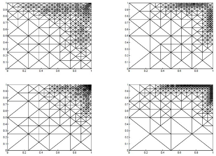
Figure 1: Top: the meshes by using ε=0.01𝜀0.01\varepsilon=0.01, δK=hKsubscript𝛿𝐾subscript𝐾\delta_{K}=h_{K}, and θ=0.3𝜃0.3\theta=0.3; Bottom: the meshes by using ε=0.0001𝜀0.0001\varepsilon=0.0001, δK=hKsubscript𝛿𝐾subscript𝐾\delta_{K}=h_{K}, and θ=0.5𝜃0.5\theta=0.5; Left: the meshes by using (ehαe2Ree2)1/2superscriptsubscript𝑒subscriptsuperscriptsubscript𝛼𝑒2superscriptsubscriptnormsubscript𝑅𝑒𝑒212\big{(}\sum_{e\in\mathcal{E}_{h}}\alpha_{e}^{2}||R_{e}||_{e}^{2}\big{)}^{1/2}; and Right: the meshes by using ε1/2σh+ε1/2uhnormsuperscript𝜀12subscript𝜎superscript𝜀12subscript𝑢||\varepsilon^{-1/2}\sigma_{h}+\varepsilon^{1/2}\nabla u_{h}|| with σhsubscript𝜎\sigma_{h} the implicit recovery flux by (3.2). The top-left, top-right, bottom-left, and bottom-right plots are meshes after 10, 8, 8, and 8 iterations with 640, 473, 635, and 749 triangles, respectively.
Remark 4.2.

Compared with the estimators developed in [15], the jump in the normal component of the flux is replaced by the residual ε1/2uh+ε1/2σhnormsuperscript𝜀12subscript𝑢superscript𝜀12subscript𝜎||\varepsilon^{1/2}\nabla u_{h}+\varepsilon^{-1/2}\sigma_{h}|| in Theorem 4.1. Moreover, a residual term K𝒯hαK2R~KK2subscript𝐾subscript𝒯superscriptsubscript𝛼𝐾2superscriptsubscriptnormsubscript~𝑅𝐾𝐾2\sum_{K\in\mathcal{T}_{h}}\alpha_{K}^{2}||\tilde{R}_{K}||_{K}^{2} and another residual term of the Neumann boundary data occur in the a posteriori error estimators. In ε1/2uh+ε1/2σhnormsuperscript𝜀12subscript𝑢superscript𝜀12subscript𝜎||\varepsilon^{1/2}\nabla u_{h}+\varepsilon^{-1/2}\sigma_{h}||, the impacts of ε𝜀\varepsilon and hh are implicitly accounted, which however are expressed explicitly in αesubscript𝛼𝑒\alpha_{e}, and hence in (ehαe2Ree2)1/2superscriptsubscript𝑒subscriptsuperscriptsubscript𝛼𝑒2superscriptsubscriptnormsubscript𝑅𝑒𝑒212\big{(}\sum_{e\in\mathcal{E}_{h}}\alpha_{e}^{2}||R_{e}||_{e}^{2}\big{)}^{1/2}, in [15] (e.g., if εhe𝜀subscript𝑒\varepsilon\leq h_{e} and β=1𝛽1\beta=1, then αe=1subscript𝛼𝑒1\alpha_{e}=1). To illustrate the difference in numerical results, we provide in Figure 1 the adaptive meshes by the two estimators for Section 7 Example 1. It is observed that the quality of the meshes generated by ε1/2uh+ε1/2σhnormsuperscript𝜀12subscript𝑢superscript𝜀12subscript𝜎||\varepsilon^{1/2}\nabla u_{h}+\varepsilon^{-1/2}\sigma_{h}|| is better than that of the meshes by (ehαe2Ree2)1/2superscriptsubscript𝑒subscriptsuperscriptsubscript𝛼𝑒2superscriptsubscriptnormsubscript𝑅𝑒𝑒212\big{(}\sum_{e\in\mathcal{E}_{h}}\alpha_{e}^{2}||R_{e}||_{e}^{2}\big{)}^{1/2}.

5 Analysis of efficiency

Let 𝝉=εuh𝝉𝜀subscript𝑢\boldsymbol{\tau}=-\varepsilon\nabla u_{h}. For each eΩ𝑒subscriptΩe\in\mathcal{E}_{\Omega}, define the edge/face residual along e𝑒e by

Re:={Je(𝝉)ifeΓ,g+𝝉𝐧eifeΓN,0ifeΓD,assignsubscript𝑅𝑒casessubscript𝐽𝑒𝝉not-subset-of-nor-equalsif𝑒Γ𝑔𝝉subscript𝐧𝑒if𝑒subscriptΓ𝑁0if𝑒subscriptΓ𝐷R_{e}:=\left\{\begin{array}[]{ll}J_{e}(\boldsymbol{\tau})&\mbox{if}\ \ e\nsubseteq\Gamma,\\ g+\boldsymbol{\tau}\cdot{\bf n}_{e}&\mbox{if}\ \ e\subset\Gamma_{N},\\ 0&\mbox{if}\ \ e\subset\Gamma_{D},\end{array}\right.

where Je(𝝉)subscript𝐽𝑒𝝉J_{e}(\boldsymbol{\tau}) is defined in (5.3). Let ΠksubscriptΠ𝑘\Pi_{k} be an L2superscript𝐿2L^{2}-projection operator into Pk(K)subscript𝑃𝑘𝐾P_{k}(K) and

osch:=(K𝒯hαK2DKK2+eΓNαe2Dee2)1/2,assignsubscriptoscsuperscriptsubscript𝐾subscript𝒯superscriptsubscript𝛼𝐾2superscriptsubscriptnormsubscript𝐷𝐾𝐾2subscript𝑒subscriptΓ𝑁superscriptsubscript𝛼𝑒2superscriptsubscriptnormsubscript𝐷𝑒𝑒212{\rm osc}_{h}:=\Big{(}\sum_{K\in\mathcal{T}_{h}}\alpha_{K}^{2}||D_{K}||_{K}^{2}+\sum_{e\subset\Gamma_{N}}\alpha_{e}^{2}||D_{e}||_{e}^{2}\Big{)}^{1/2},

be an oscillation of data, where DK=RKΠkRKsubscript𝐷𝐾subscript𝑅𝐾subscriptΠ𝑘subscript𝑅𝐾D_{K}=R_{K}-\Pi_{k}R_{K} for every K𝒯h𝐾subscript𝒯K\in\mathcal{T}_{h}, and De=ReΠkResubscript𝐷𝑒subscript𝑅𝑒subscriptΠ𝑘subscript𝑅𝑒D_{e}=R_{e}-\Pi_{k}R_{e} for each eΓN𝑒subscriptΓ𝑁e\subset\Gamma_{N}. The following efficient estimate is found in [15].

Lemma 5.1.

Let u𝑢u and uhsubscript𝑢u_{h} be the solutions to problems (2.2) and (2.4), respectively. Then the error is bounded from below by

(K𝒯h(αK2RKK2+eKαe2Ree2))1/2|uuh|+osch.precedes-or-equalssuperscriptsubscript𝐾subscript𝒯superscriptsubscript𝛼𝐾2superscriptsubscriptnormsubscript𝑅𝐾𝐾2subscript𝑒𝐾superscriptsubscript𝛼𝑒2superscriptsubscriptnormsubscript𝑅𝑒𝑒212subscriptnorm𝑢subscript𝑢subscriptosc\Big{(}\sum_{K\in\mathcal{T}_{h}}\big{(}\alpha_{K}^{2}||R_{K}||_{K}^{2}+\sum_{e\subset\partial K}\alpha_{e}^{2}||R_{e}||_{e}^{2}\big{)}\Big{)}^{1/2}\preceq|||u-u_{h}|||_{*}+{\rm osc}_{h}. (5.1)
Lemma 5.2.

Let u𝑢u and uhsubscript𝑢u_{h} be the solutions to (2.2) and (2.4), respectively. If σ^RT0(uh)subscript^𝜎𝑅subscript𝑇0subscript𝑢\hat{\sigma}_{RT_{0}}(u_{h}) is the explicit recovery flux given by (3.3), then it holds

ε1/2σ^RT0(uh)+ε1/2uh|uuh|+osch.precedes-or-equalsnormsuperscript𝜀12subscript^𝜎𝑅subscript𝑇0subscript𝑢superscript𝜀12subscript𝑢subscriptnorm𝑢subscript𝑢subscriptosc||\varepsilon^{-1/2}\hat{\sigma}_{RT_{0}}(u_{h})+\varepsilon^{1/2}\nabla u_{h}||\preceq|||u-u_{h}|||_{*}+{\rm osc}_{h}. (5.2)
Proof.

For any element K𝒯h𝐾subscript𝒯K\in\mathcal{T}_{h} and an edge/face eK𝑒𝐾e\subset\partial K, let 𝐧esubscript𝐧𝑒{\bf n}_{e} be the outward unit vector normal to K𝐾\partial K. Note that 𝝉=εuh𝝉𝜀subscript𝑢\boldsymbol{\tau}=-\varepsilon\nabla u_{h} on K𝐾K is a constant vector. Let 𝝉e,K=(𝝉|K𝐧e)|esubscript𝝉𝑒𝐾evaluated-atevaluated-at𝝉𝐾subscript𝐧𝑒𝑒\boldsymbol{\tau}_{e,K}=(\boldsymbol{\tau}|_{K}\cdot{\bf n}_{e})|_{e} be the normal component of 𝝉𝝉\boldsymbol{\tau} on e𝑒e. There holds the representation in RT0𝑅subscript𝑇0RT_{0}: 𝝉=eK𝝉e,Kϕe(𝐱)𝝉subscript𝑒𝐾subscript𝝉𝑒𝐾subscriptitalic-ϕ𝑒𝐱\boldsymbol{\tau}=\sum_{e\subset\partial K}\boldsymbol{\tau}_{e,K}\phi_{e}({\bf x}). Then, for 𝐱K𝐱𝐾{\bf x}\in K, (3.3) and (3.4) give

σ^RT0(uh)𝝉=eKΩ(σ^e𝝉|e𝐧e)ϕe(𝐱)=eKΓ(1γe)Je(𝝉)ϕe(𝐱),subscript^𝜎𝑅subscript𝑇0subscript𝑢𝝉subscript𝑒𝐾subscriptΩsubscript^𝜎𝑒evaluated-at𝝉𝑒subscript𝐧𝑒subscriptitalic-ϕ𝑒𝐱subscript𝑒𝐾Γ1subscript𝛾𝑒subscript𝐽𝑒𝝉subscriptitalic-ϕ𝑒𝐱\hat{\sigma}_{RT_{0}}(u_{h})-\boldsymbol{\tau}=\sum_{e\subset\partial K\cap\mathcal{E}_{\Omega}}(\hat{\sigma}_{e}-\boldsymbol{\tau}|_{e}\cdot{\bf n}_{e})\phi_{e}({\bf x})=\sum_{e\subset\partial K\setminus\Gamma}(1-\gamma_{e})J_{e}(\boldsymbol{\tau})\phi_{e}({\bf x}),

where, for the two elements Ke+superscriptsubscript𝐾𝑒K_{e}^{+} and Kesuperscriptsubscript𝐾𝑒K_{e}^{-} sharing e𝑒e,

Je(𝝉)=(𝝉|Ke+𝝉|Ke)𝐧e.subscript𝐽𝑒𝝉evaluated-at𝝉superscriptsubscript𝐾𝑒evaluated-at𝝉superscriptsubscript𝐾𝑒subscript𝐧𝑒J_{e}(\boldsymbol{\tau})=(\boldsymbol{\tau}|_{K_{e}^{+}}-\boldsymbol{\tau}|_{K_{e}^{-}})\cdot{\bf n}_{e}. (5.3)

This identity implies

ε1/2(σ^RT0(uh)𝝉)K2eKΓ(1γe)2εJe(𝝉)ϕe(𝐱)K2precedes-or-equalssuperscriptsubscriptnormsuperscript𝜀12subscript^𝜎𝑅subscript𝑇0subscript𝑢𝝉𝐾2subscript𝑒𝐾Γsuperscript1subscript𝛾𝑒2𝜀superscriptsubscriptnormsubscript𝐽𝑒𝝉subscriptitalic-ϕ𝑒𝐱𝐾2\displaystyle||\varepsilon^{-1/2}(\hat{\sigma}_{RT_{0}}(u_{h})-\boldsymbol{\tau})||_{K}^{2}\preceq\sum_{e\subset\partial K\setminus\Gamma}\frac{(1-\gamma_{e})^{2}}{\varepsilon}||J_{e}(\boldsymbol{\tau})\phi_{e}({\bf x})||_{K}^{2}
\displaystyle\leq eKΓ(1γe)2ε|Je(𝝉)|2ϕe(𝐱)K2eKΓ(1γe)2εJe(𝝉)e2he,precedes-or-equalssubscript𝑒𝐾Γsuperscript1subscript𝛾𝑒2𝜀superscriptsubscript𝐽𝑒𝝉2superscriptsubscriptnormsubscriptitalic-ϕ𝑒𝐱𝐾2subscript𝑒𝐾Γsuperscript1subscript𝛾𝑒2𝜀superscriptsubscriptnormsubscript𝐽𝑒𝝉𝑒2subscript𝑒\displaystyle\sum_{e\subset\partial K\setminus\Gamma}\frac{(1-\gamma_{e})^{2}}{\varepsilon}|J_{e}(\boldsymbol{\tau})|^{2}||\phi_{e}({\bf x})||_{K}^{2}\preceq\sum_{e\subset\partial K\setminus\Gamma}\frac{(1-\gamma_{e})^{2}}{\varepsilon}||J_{e}(\boldsymbol{\tau})||_{e}^{2}h_{e}, (5.4)

where, in the last step, we employ the fact that Je(𝝉)subscript𝐽𝑒𝝉J_{e}(\boldsymbol{\tau}) is constant and ϕe(𝐱)K2|K|precedes-or-equalssuperscriptsubscriptnormsubscriptitalic-ϕ𝑒𝐱𝐾2𝐾||\phi_{e}({\bf x})||_{K}^{2}\preceq|K|.

Now, for each eΩ𝑒subscriptΩe\in\mathcal{E}_{\Omega} we choose

γe=1αeε1/2he1/2subscript𝛾𝑒1subscript𝛼𝑒superscript𝜀12superscriptsubscript𝑒12\gamma_{e}=1-\alpha_{e}\varepsilon^{1/2}h_{e}^{-1/2} (5.5)

so that (1γe)2he/ε=1superscript1subscript𝛾𝑒2subscript𝑒𝜀1{(1-\gamma_{e})^{2}h_{e}}/{\varepsilon}=1. Since αehe/εsubscript𝛼𝑒subscript𝑒𝜀\alpha_{e}\leq\sqrt{h_{e}/\varepsilon}, thus 0γe<10subscript𝛾𝑒10\leq\gamma_{e}<1. This choice together with the definition of the edge//face residual Resubscript𝑅𝑒R_{e} leads to

(1γe)2εheJe(𝝉)e2αe2Ree2,superscript1subscript𝛾𝑒2𝜀subscript𝑒superscriptsubscriptnormsubscript𝐽𝑒𝝉𝑒2superscriptsubscript𝛼𝑒2superscriptsubscriptnormsubscript𝑅𝑒𝑒2\frac{(1-\gamma_{e})^{2}}{\varepsilon}h_{e}||J_{e}(\boldsymbol{\tau})||_{e}^{2}\leq\alpha_{e}^{2}||R_{e}||_{e}^{2},

which, with (5.4), implies

ε1/2σ^RT0(uh)+ε1/2uhK2eKΓαe2Ree2.precedes-or-equalssuperscriptsubscriptnormsuperscript𝜀12subscript^𝜎𝑅subscript𝑇0subscript𝑢superscript𝜀12subscript𝑢𝐾2subscript𝑒𝐾Γsuperscriptsubscript𝛼𝑒2superscriptsubscriptnormsubscript𝑅𝑒𝑒2||\varepsilon^{-1/2}\hat{\sigma}_{RT_{0}}(u_{h})+\varepsilon^{1/2}\nabla u_{h}||_{K}^{2}\preceq\displaystyle\sum_{e\subset\partial K\setminus\Gamma}\alpha_{e}^{2}||R_{e}||_{e}^{2}. (5.6)

Summing up (5.6) over all K𝒯h𝐾subscript𝒯K\in\mathcal{T}_{h}, we obtain

ε1/2σ^RT0(uh)+ε1/2uh2K𝒯heKΓαe2Ree2K𝒯heKαe2Ree2.precedes-or-equalssuperscriptnormsuperscript𝜀12subscript^𝜎𝑅subscript𝑇0subscript𝑢superscript𝜀12subscript𝑢2subscript𝐾subscript𝒯subscript𝑒𝐾Γsuperscriptsubscript𝛼𝑒2superscriptsubscriptnormsubscript𝑅𝑒𝑒2precedes-or-equalssubscript𝐾subscript𝒯subscript𝑒𝐾superscriptsubscript𝛼𝑒2superscriptsubscriptnormsubscript𝑅𝑒𝑒2||\varepsilon^{-1/2}\hat{\sigma}_{RT_{0}}(u_{h})+\varepsilon^{1/2}\nabla u_{h}||^{2}\preceq\sum_{K\in\mathcal{T}_{h}}\sum_{e\subset\partial K\setminus\Gamma}\alpha_{e}^{2}||R_{e}||_{e}^{2}\preceq\sum_{K\in\mathcal{T}_{h}}\sum_{e\subset\partial K}\alpha_{e}^{2}||R_{e}||_{e}^{2}. (5.7)

The desired estimate (5.2) follows from (5.7) and (5.1). ∎

Lemma 5.3.

Under the assumption of Lemma 5.2, if σνsubscript𝜎𝜈\sigma_{\nu} is the implicit recovery flux obtained by (3.2), then it holds

ε1/2σν+ε1/2uh|uuh|+osch.precedes-or-equalsnormsuperscript𝜀12subscript𝜎𝜈superscript𝜀12subscript𝑢subscriptnorm𝑢subscript𝑢subscriptosc||\varepsilon^{-1/2}\sigma_{\nu}+\varepsilon^{1/2}\nabla u_{h}||\preceq|||u-u_{h}|||_{*}+{\rm osc}_{h}. (5.8)
Proof.

For all τ𝒱𝜏𝒱\tau\in\mathcal{V}, (3.2) implies

(ε1/2σν+ε1/2uh,ε1/2τ)=0,superscript𝜀12subscript𝜎𝜈superscript𝜀12subscript𝑢superscript𝜀12𝜏0(\varepsilon^{-1/2}\sigma_{\nu}+\varepsilon^{1/2}\nabla u_{h},\varepsilon^{-1/2}\tau)=0,

which results in

ε1/2σν+ε1/2uh2=(ε12σν+ε12uh,ε12(σντ)+ε12τ+ε12uh)superscriptnormsuperscript𝜀12subscript𝜎𝜈superscript𝜀12subscript𝑢2superscript𝜀12subscript𝜎𝜈superscript𝜀12subscript𝑢superscript𝜀12subscript𝜎𝜈𝜏superscript𝜀12𝜏superscript𝜀12subscript𝑢\displaystyle||\varepsilon^{-1/2}\sigma_{\nu}+\varepsilon^{1/2}\nabla u_{h}||^{2}=(\varepsilon^{-\frac{1}{2}}\sigma_{\nu}+\varepsilon^{\frac{1}{2}}\nabla u_{h},\varepsilon^{-\frac{1}{2}}(\sigma_{\nu}-\tau)+\varepsilon^{-\frac{1}{2}}\tau+\varepsilon^{\frac{1}{2}}\nabla u_{h})
=\displaystyle= (ε1/2σν+ε1/2uh,ε1/2τ+ε1/2uh)ε1/2σν+ε1/2uhε1/2τ+ε1/2uh.superscript𝜀12subscript𝜎𝜈superscript𝜀12subscript𝑢superscript𝜀12𝜏superscript𝜀12subscript𝑢normsuperscript𝜀12subscript𝜎𝜈superscript𝜀12subscript𝑢normsuperscript𝜀12𝜏superscript𝜀12subscript𝑢\displaystyle(\varepsilon^{-1/2}\sigma_{\nu}+\varepsilon^{1/2}\nabla u_{h},\varepsilon^{-1/2}\tau+\varepsilon^{1/2}\nabla u_{h})\leq||\varepsilon^{-1/2}\sigma_{\nu}+\varepsilon^{1/2}\nabla u_{h}||||\varepsilon^{-1/2}\tau+\varepsilon^{1/2}\nabla u_{h}||.

Dividing by ε1/2σν+ε1/2uhnormsuperscript𝜀12subscript𝜎𝜈superscript𝜀12subscript𝑢||\varepsilon^{-1/2}\sigma_{\nu}+\varepsilon^{1/2}\nabla u_{h}||, we get

ε1/2σν+ε1/2uhε1/2τ+ε1/2uhnormsuperscript𝜀12subscript𝜎𝜈superscript𝜀12subscript𝑢normsuperscript𝜀12𝜏superscript𝜀12subscript𝑢||\varepsilon^{-1/2}\sigma_{\nu}+\varepsilon^{1/2}\nabla u_{h}||\leq||\varepsilon^{-1/2}\tau+\varepsilon^{1/2}\nabla u_{h}||

for all τ𝒱𝜏𝒱\tau\in\mathcal{V}, which implies

ε1/2σν+ε1/2uh=minτ𝒱ε1/2τ+ε1/2uh.normsuperscript𝜀12subscript𝜎𝜈superscript𝜀12subscript𝑢subscript𝜏𝒱normsuperscript𝜀12𝜏superscript𝜀12subscript𝑢||\varepsilon^{-1/2}\sigma_{\nu}+\varepsilon^{1/2}\nabla u_{h}||=\min_{\tau\in\mathcal{V}}||\varepsilon^{-1/2}\tau+\varepsilon^{1/2}\nabla u_{h}||. (5.9)

The assertion (5.8) follows from the fact that RT0BDM1𝑅subscript𝑇0𝐵𝐷subscript𝑀1RT_{0}\subset BDM_{1}, (5.9), and Lemma 5.2. ∎

Lemma 5.4.

Under the assumption of Lemma 5.2, if σνsubscript𝜎𝜈\sigma_{\nu} is the implicit recovery flux obtained by (3.2), then it holds

(eΓNαe2(σν+εuh)𝐧e2)1/2ε1/2σν+ε1/2uh.precedes-or-equalssuperscriptsubscript𝑒subscriptΓ𝑁superscriptsubscript𝛼𝑒2superscriptsubscriptnormsubscript𝜎𝜈𝜀subscript𝑢𝐧𝑒212normsuperscript𝜀12subscript𝜎𝜈superscript𝜀12subscript𝑢\Big{(}\sum_{e\subset\Gamma_{N}}\alpha_{e}^{2}||(\sigma_{\nu}+\varepsilon\nabla u_{h})\cdot{\bf n}||_{e}^{2}\Big{)}^{1/2}\preceq||\varepsilon^{-1/2}\sigma_{\nu}+\varepsilon^{1/2}\nabla u_{h}||. (5.10)
Proof.

Using trace theorem, inverse estimate, shape regularity of element, and the fact αehe1/2/εsubscript𝛼𝑒superscriptsubscript𝑒12𝜀\alpha_{e}\leq h_{e}^{1/2}/\sqrt{\varepsilon}, we have for eΓNK𝑒subscriptΓ𝑁𝐾e\subset\Gamma_{N}\cap\partial K

αe(σν+εuh)𝐧eαehK1/2σν+εuhKε1/2σν+ε1/2uhK.precedes-or-equalssubscript𝛼𝑒subscriptnormsubscript𝜎𝜈𝜀subscript𝑢𝐧𝑒subscript𝛼𝑒superscriptsubscript𝐾12subscriptnormsubscript𝜎𝜈𝜀subscript𝑢𝐾precedes-or-equalssubscriptnormsuperscript𝜀12subscript𝜎𝜈superscript𝜀12subscript𝑢𝐾\alpha_{e}||(\sigma_{\nu}+\varepsilon\nabla u_{h})\cdot{\bf n}||_{e}\preceq\alpha_{e}h_{K}^{-1/2}||\sigma_{\nu}+\varepsilon\nabla u_{h}||_{K}\preceq||\varepsilon^{-1/2}\sigma_{\nu}+\varepsilon^{1/2}\nabla u_{h}||_{K}.

Summing the above inequality over all eΓN𝑒subscriptΓ𝑁e\subset\Gamma_{N}, we obtain the desired estimate (5.10). ∎

Moreover, we have the following estimate.

Lemma 5.5.

Let σhsubscript𝜎\sigma_{h} be the flux recovery obtained by the implicit approximation (3.2) or the explicit approximation (3.3). Then it holds

(K𝒯hαK2R~KK2)1/2(K𝒯hαK2RKK2)1/2+ε1/2uh+ε1/2σh.precedes-or-equalssuperscriptsubscript𝐾subscript𝒯superscriptsubscript𝛼𝐾2superscriptsubscriptnormsubscript~𝑅𝐾𝐾212superscriptsubscript𝐾subscript𝒯superscriptsubscript𝛼𝐾2superscriptsubscriptnormsubscript𝑅𝐾𝐾212normsuperscript𝜀12subscript𝑢superscript𝜀12subscript𝜎\Big{(}\sum_{K\in\mathcal{T}_{h}}\alpha_{K}^{2}||\tilde{R}_{K}||_{K}^{2}\Big{)}^{1/2}\preceq\Big{(}\sum_{K\in\mathcal{T}_{h}}\alpha_{K}^{2}||R_{K}||_{K}^{2}\Big{)}^{1/2}+||\varepsilon^{1/2}\nabla u_{h}+\varepsilon^{-1/2}\sigma_{h}||. (5.11)
Proof.

For each K𝒯h𝐾subscript𝒯K\in\mathcal{T}_{h}, it follows from triangle inequality and inverse estimate that

R~KKRKK+εuh+σhKRKK+hK1ε1/2ε1/2uh+ε1/2σhK.subscriptnormsubscript~𝑅𝐾𝐾subscriptnormsubscript𝑅𝐾𝐾subscriptnorm𝜀subscript𝑢subscript𝜎𝐾missing-subexpressionprecedes-or-equalssubscriptnormsubscript𝑅𝐾𝐾superscriptsubscript𝐾1superscript𝜀12subscriptnormsuperscript𝜀12subscript𝑢superscript𝜀12subscript𝜎𝐾\begin{array}[]{lll}||\tilde{R}_{K}||_{K}&\leq&||R_{K}||_{K}+||\varepsilon\triangle u_{h}+\nabla\cdot\sigma_{h}||_{K}\\ &\preceq&||R_{K}||_{K}+h_{K}^{-1}\varepsilon^{1/2}||\varepsilon^{1/2}\nabla u_{h}+\varepsilon^{-1/2}\sigma_{h}||_{K}.\end{array}

We get from the fact αKhK/εsubscript𝛼𝐾subscript𝐾𝜀\alpha_{K}\leq h_{K}/\sqrt{\varepsilon} that

αKR~KKαKRKK+ε1/2uh+ε1/2σhK.precedes-or-equalssubscript𝛼𝐾subscriptnormsubscript~𝑅𝐾𝐾subscript𝛼𝐾subscriptnormsubscript𝑅𝐾𝐾subscriptnormsuperscript𝜀12subscript𝑢superscript𝜀12subscript𝜎𝐾\alpha_{K}||\tilde{R}_{K}||_{K}\preceq\alpha_{K}||R_{K}||_{K}+||\varepsilon^{1/2}\nabla u_{h}+\varepsilon^{-1/2}\sigma_{h}||_{K}.

Summing up the above inequality over all K𝒯h𝐾subscript𝒯K\in\mathcal{T}_{h}, we obtain

K𝒯hαK2R~KK2K𝒯hαK2RKK2+ε1/2uh+ε1/2σh2,precedes-or-equalssubscript𝐾subscript𝒯superscriptsubscript𝛼𝐾2superscriptsubscriptnormsubscript~𝑅𝐾𝐾2subscript𝐾subscript𝒯superscriptsubscript𝛼𝐾2superscriptsubscriptnormsubscript𝑅𝐾𝐾2superscriptnormsuperscript𝜀12subscript𝑢superscript𝜀12subscript𝜎2\displaystyle\sum_{K\in\mathcal{T}_{h}}\alpha_{K}^{2}||\tilde{R}_{K}||_{K}^{2}\preceq\sum_{K\in\mathcal{T}_{h}}\alpha_{K}^{2}||R_{K}||_{K}^{2}+||\varepsilon^{1/2}\nabla u_{h}+\varepsilon^{-1/2}\sigma_{h}||^{2},

which results in the desired estimate (5.11). ∎

Collecting Lemma 5.1-5.5, we obtain the global lower bound estimate.

Theorem 5.6.

Let u𝑢u and uhsubscript𝑢u_{h} be the solutions to (2.2) and (2.4), respectively. Let ΦΦ\Phi be defined in (4.2). If σhsubscript𝜎\sigma_{h} is the recovery flux obtained by the explicit approximation (3.3), i.e., σh=σ^RT0(uh)subscript𝜎subscript^𝜎𝑅subscript𝑇0subscript𝑢\sigma_{h}=\hat{\sigma}_{RT_{0}}(u_{h}), then

Φ+(eΓNαe2gεuh𝐧e2)1/2|uuh|+osch.precedes-or-equalsΦsuperscriptsubscript𝑒subscriptΓ𝑁superscriptsubscript𝛼𝑒2superscriptsubscriptnorm𝑔𝜀subscript𝑢𝐧𝑒212subscriptnorm𝑢subscript𝑢subscriptosc\Phi+\Big{(}\sum_{e\subset\Gamma_{N}}\alpha_{e}^{2}||g-\varepsilon\nabla u_{h}\cdot{\bf n}||_{e}^{2}\Big{)}^{1/2}\preceq|||u-u_{h}|||_{*}+{\rm osc}_{h}. (5.12)

If σhsubscript𝜎\sigma_{h} is the recovery flux obtained by the implicit approximation (3.2), i.e., σh=σνsubscript𝜎subscript𝜎𝜈\sigma_{h}=\sigma_{\nu}, then

Φ+(eΓNαe2(gεuh𝐧e2+(σh+εuh)𝐧e2))12|uuh|+osch.precedes-or-equalsΦsuperscriptsubscript𝑒subscriptΓ𝑁superscriptsubscript𝛼𝑒2superscriptsubscriptnorm𝑔𝜀subscript𝑢𝐧𝑒2superscriptsubscriptnormsubscript𝜎𝜀subscript𝑢𝐧𝑒212subscriptnorm𝑢subscript𝑢subscriptosc\Phi+\Big{(}\sum_{e\subset\Gamma_{N}}\alpha_{e}^{2}(||g-\varepsilon\nabla u_{h}\cdot{\bf n}||_{e}^{2}+||(\sigma_{h}+\varepsilon\nabla u_{h})\cdot{\bf n}||_{e}^{2})\Big{)}^{\frac{1}{2}}\preceq|||u-u_{h}|||_{*}+{\rm osc}_{h}. (5.13)
Proof.

It follows from Lemmas 5.2-5.3 that

ε1/2uh+ε1/2σh2|uuh|2+osch.precedes-or-equalssuperscriptnormsuperscript𝜀12subscript𝑢superscript𝜀12subscript𝜎2superscriptsubscriptnorm𝑢subscript𝑢2subscriptosc||\varepsilon^{1/2}\nabla u_{h}+\varepsilon^{-1/2}\sigma_{h}||^{2}\preceq|||u-u_{h}|||_{*}^{2}+{\rm osc}_{h}. (5.14)

If σh=σ^RT0(uh)subscript𝜎subscript^𝜎𝑅subscript𝑇0subscript𝑢\sigma_{h}=\hat{\sigma}_{RT_{0}}(u_{h}), we get from Lemma 5.1 and Lemma 5.5 that

K𝒯hαK2(RKK2+R~KK2)+eΓNαe2gεuh𝐧e2subscript𝐾subscript𝒯superscriptsubscript𝛼𝐾2superscriptsubscriptnormsubscript𝑅𝐾𝐾2superscriptsubscriptnormsubscript~𝑅𝐾𝐾2subscript𝑒subscriptΓ𝑁superscriptsubscript𝛼𝑒2superscriptsubscriptnorm𝑔𝜀subscript𝑢𝐧𝑒2\displaystyle\sum_{K\in\mathcal{T}_{h}}\alpha_{K}^{2}(||R_{K}||_{K}^{2}+||\tilde{R}_{K}||_{K}^{2})+\sum_{e\subset\Gamma_{N}}\alpha_{e}^{2}||g-\varepsilon\nabla u_{h}\cdot{\bf n}||_{e}^{2}
\displaystyle\leq K𝒯h(αK2RKK2+eKαe2Ree2)+K𝒯hαK2R~KK2subscript𝐾subscript𝒯superscriptsubscript𝛼𝐾2superscriptsubscriptnormsubscript𝑅𝐾𝐾2subscript𝑒𝐾superscriptsubscript𝛼𝑒2superscriptsubscriptnormsubscript𝑅𝑒𝑒2subscript𝐾subscript𝒯superscriptsubscript𝛼𝐾2superscriptsubscriptnormsubscript~𝑅𝐾𝐾2\displaystyle\sum_{K\in\mathcal{T}_{h}}(\alpha_{K}^{2}||R_{K}||_{K}^{2}+\sum_{e\subset\partial K}\alpha_{e}^{2}||R_{e}||_{e}^{2})+\sum_{K\in\mathcal{T}_{h}}\alpha_{K}^{2}||\tilde{R}_{K}||_{K}^{2}
precedes-or-equals\displaystyle\preceq K𝒯h(αK2RKK2+eKαe2Ree2)+ε1/2uh+ε1/2σh2subscript𝐾subscript𝒯superscriptsubscript𝛼𝐾2superscriptsubscriptnormsubscript𝑅𝐾𝐾2subscript𝑒𝐾superscriptsubscript𝛼𝑒2superscriptsubscriptnormsubscript𝑅𝑒𝑒2superscriptnormsuperscript𝜀12subscript𝑢superscript𝜀12subscript𝜎2\displaystyle\sum_{K\in\mathcal{T}_{h}}(\alpha_{K}^{2}||R_{K}||_{K}^{2}+\sum_{e\subset\partial K}\alpha_{e}^{2}||R_{e}||_{e}^{2})+||\varepsilon^{1/2}\nabla u_{h}+\varepsilon^{-1/2}\sigma_{h}||^{2}
precedes-or-equals\displaystyle\preceq |uuh|2+osch2+ε1/2uh+ε1/2σh2.superscriptsubscriptnorm𝑢subscript𝑢2superscriptsubscriptosc2superscriptnormsuperscript𝜀12subscript𝑢superscript𝜀12subscript𝜎2\displaystyle~{}|||u-u_{h}|||_{*}^{2}+{\rm osc}_{h}^{2}+||\varepsilon^{1/2}\nabla u_{h}+\varepsilon^{-1/2}\sigma_{h}||^{2}. (5.15)

The assertion (5.12) follows from a combination of (5.14) and (5.15). If σh=σνsubscript𝜎subscript𝜎𝜈\sigma_{h}=\sigma_{\nu}, then, similarly, we have from Lemma 5.1 and Lemmas 5.4-5.5 that

K𝒯hαK2(RKK2+R~KK2)+eΓNαe2(gεuh𝐧e2+(σh+εuh)𝐧e2)subscript𝐾subscript𝒯superscriptsubscript𝛼𝐾2superscriptsubscriptnormsubscript𝑅𝐾𝐾2superscriptsubscriptnormsubscript~𝑅𝐾𝐾2subscript𝑒subscriptΓ𝑁superscriptsubscript𝛼𝑒2superscriptsubscriptnorm𝑔𝜀subscript𝑢𝐧𝑒2superscriptsubscriptnormsubscript𝜎𝜀subscript𝑢𝐧𝑒2\displaystyle\sum_{K\in\mathcal{T}_{h}}\alpha_{K}^{2}(||R_{K}||_{K}^{2}+||\tilde{R}_{K}||_{K}^{2})+\sum_{e\subset\Gamma_{N}}\alpha_{e}^{2}(||g-\varepsilon\nabla u_{h}\cdot{\bf n}||_{e}^{2}+||(\sigma_{h}+\varepsilon\nabla u_{h})\cdot{\bf n}||_{e}^{2})
precedes-or-equals\displaystyle\preceq |uuh|2+osch2+ε1/2uh+ε1/2σh2.superscriptsubscriptnorm𝑢subscript𝑢2superscriptsubscriptosc2superscriptnormsuperscript𝜀12subscript𝑢superscript𝜀12subscript𝜎2\displaystyle~{}|||u-u_{h}|||_{*}^{2}+{\rm osc}_{h}^{2}+||\varepsilon^{1/2}\nabla u_{h}+\varepsilon^{-1/2}\sigma_{h}||^{2}.

The estimate (5.13) follows from the above inequality and (5.14). ∎

6 A stabilization H(div)𝐻divH({\rm div}) recovery

Let uhVhsubscript𝑢subscript𝑉u_{h}\in V_{h} be the approximation of the solution u𝑢u to (1.1). A stabilization H(div)𝐻divH({\rm div}) recovery procedure is to find σ𝒯𝒱subscript𝜎𝒯𝒱\sigma_{\mathcal{T}}\in\mathcal{V} such that

(ε1σ𝒯,τν)+K𝒯hγK(σ𝒯,τν)Ksuperscript𝜀1subscript𝜎𝒯subscript𝜏𝜈subscript𝐾subscript𝒯subscript𝛾𝐾subscriptsubscript𝜎𝒯subscript𝜏𝜈𝐾\displaystyle(\varepsilon^{-1}\sigma_{\mathcal{T}},\tau_{\nu})+\sum_{K\in\mathcal{T}_{h}}\gamma_{K}(\nabla\cdot\sigma_{\mathcal{T}},\nabla\cdot\tau_{\nu})_{K}
=\displaystyle= (uh,τν)+K𝒯hγK(f𝐚uhbuh,τν)Kτν𝒱,subscript𝑢subscript𝜏𝜈subscript𝐾subscript𝒯subscript𝛾𝐾subscript𝑓𝐚subscript𝑢𝑏subscript𝑢subscript𝜏𝜈𝐾for-allsubscript𝜏𝜈𝒱\displaystyle-(\nabla u_{h},\tau_{\nu})+\sum_{K\in\mathcal{T}_{h}}\gamma_{K}(f-{\bf a}\cdot\nabla u_{h}-bu_{h},\nabla\cdot\tau_{\nu})_{K}\quad\forall\tau_{\nu}\in\mathcal{V}, (6.1)

where γKsubscript𝛾𝐾\gamma_{K} is a stabilization parameter to be determined in below. Recalling the exact flux σ=εu𝜎𝜀𝑢\sigma=-\varepsilon\nabla u, define the approximation error of the flux recovery by

σσ𝒯B,Ω2:=(ε1(σσ𝒯),σσ𝒯)+K𝒯hγK((σσ𝒯),(σσ𝒯))K.assignsuperscriptsubscriptnorm𝜎subscript𝜎𝒯𝐵Ω2superscript𝜀1𝜎subscript𝜎𝒯𝜎subscript𝜎𝒯subscript𝐾subscript𝒯subscript𝛾𝐾subscript𝜎subscript𝜎𝒯𝜎subscript𝜎𝒯𝐾||\sigma-\sigma_{\mathcal{T}}||_{B,\Omega}^{2}:=(\varepsilon^{-1}(\sigma-\sigma_{\mathcal{T}}),\sigma-\sigma_{\mathcal{T}})+\displaystyle\sum_{K\in\mathcal{T}_{h}}\gamma_{K}(\nabla\cdot(\sigma-\sigma_{\mathcal{T}}),\nabla\cdot(\sigma-\sigma_{\mathcal{T}}))_{K}.
Theorem 6.1.

The following a priori error bound for the approximation error of the H(div)𝐻divH({\rm div}) recovery flux holds

σσ𝒯B,Ωinfτν𝒱στνB,Ω+uuhε.precedes-or-equalssubscriptnorm𝜎subscript𝜎𝒯𝐵Ωsubscriptinfimumsubscript𝜏𝜈𝒱subscriptnorm𝜎subscript𝜏𝜈𝐵Ωsubscriptnorm𝑢subscript𝑢𝜀||\sigma-\sigma_{\mathcal{T}}||_{B,\Omega}\preceq\inf_{\tau_{\nu}\in\mathcal{V}}||\sigma-\tau_{\nu}||_{B,\Omega}+||u-u_{h}||_{\varepsilon}. (6.2)
Proof.

Note that the exact flux σ𝜎\sigma satisfies, for all τH(div;Ω)𝜏𝐻divΩ\tau\in H({\rm div};\Omega),

(ε1σ,τ)+K𝒯hγK(σ,τ)K=(u,τ)+K𝒯hγK(f𝐚ubu,τ)K.superscript𝜀1𝜎𝜏subscript𝐾subscript𝒯subscript𝛾𝐾subscript𝜎𝜏𝐾𝑢𝜏subscript𝐾subscript𝒯subscript𝛾𝐾subscript𝑓𝐚𝑢𝑏𝑢𝜏𝐾(\varepsilon^{-1}\sigma,\tau)+\displaystyle\sum_{K\in\mathcal{T}_{h}}\gamma_{K}(\nabla\cdot\sigma,\nabla\cdot\tau)_{K}=-(\nabla u,\tau)+\displaystyle\sum_{K\in\mathcal{T}_{h}}\gamma_{K}(f-{\bf a}\cdot\nabla u-bu,\nabla\cdot\tau)_{K}.

For all τν𝒱subscript𝜏𝜈𝒱\tau_{\nu}\in\mathcal{V}, This identity and (6.1) give the error equation

(ε1(σσ𝒯),τν)+K𝒯hγK((σσ𝒯),τν)Ksuperscript𝜀1𝜎subscript𝜎𝒯subscript𝜏𝜈subscript𝐾subscript𝒯subscript𝛾𝐾subscript𝜎subscript𝜎𝒯subscript𝜏𝜈𝐾\displaystyle(\varepsilon^{-1}(\sigma-\sigma_{\mathcal{T}}),\tau_{\nu})+\sum_{K\in\mathcal{T}_{h}}\gamma_{K}(\nabla\cdot(\sigma-\sigma_{\mathcal{T}}),\nabla\cdot\tau_{\nu})_{K}
=\displaystyle= ((uuh),τν)K𝒯hγK(𝐚(uuh)+b(uuh),τν)K𝑢subscript𝑢subscript𝜏𝜈subscript𝐾subscript𝒯subscript𝛾𝐾subscript𝐚𝑢subscript𝑢𝑏𝑢subscript𝑢subscript𝜏𝜈𝐾\displaystyle-(\nabla(u-u_{h}),\tau_{\nu})-\sum_{K\in\mathcal{T}_{h}}\gamma_{K}({\bf a}\cdot\nabla(u-u_{h})+b(u-u_{h}),\nabla\cdot\tau_{\nu})_{K} (6.3)

which implies

||σ\displaystyle||\sigma- σ𝒯||B,Ω2=(ε1(σσ𝒯),στν)+K𝒯hγK((σσ𝒯),(στν))K\displaystyle\sigma_{\mathcal{T}}||_{B,\Omega}^{2}=~{}(\varepsilon^{-1}(\sigma-\sigma_{\mathcal{T}}),\sigma-\tau_{\nu})+\sum_{K\in\mathcal{T}_{h}}\gamma_{K}(\nabla\cdot(\sigma-\sigma_{\mathcal{T}}),\nabla\cdot(\sigma-\tau_{\nu}))_{K}
((uuh),τνσ𝒯)K𝒯hγK(𝐚(uuh)+b(uuh),(τνσ𝒯))K.𝑢subscript𝑢subscript𝜏𝜈subscript𝜎𝒯subscript𝐾subscript𝒯subscript𝛾𝐾subscript𝐚𝑢subscript𝑢𝑏𝑢subscript𝑢subscript𝜏𝜈subscript𝜎𝒯𝐾\displaystyle-(\nabla(u-u_{h}),\tau_{\nu}-\sigma_{\mathcal{T}})-\sum_{K\in\mathcal{T}_{h}}\gamma_{K}({\bf a}\cdot\nabla(u-u_{h})+b(u-u_{h}),\nabla\cdot(\tau_{\nu}-\sigma_{\mathcal{T}}))_{K}.

Using (1.2) and Cauchy-Schwartz inequality, we arrive at

||σ\displaystyle||\sigma- σ𝒯||B,Ω2||σσ𝒯||B,Ω||στν||B,Ω+||uuh||ε||τνσ𝒯||B,Ω\displaystyle\sigma_{\mathcal{T}}||_{B,\Omega}^{2}\leq||\sigma-\sigma_{\mathcal{T}}||_{B,\Omega}||\sigma-\tau_{\nu}||_{B,\Omega}+||u-u_{h}||_{\varepsilon}||\tau_{\nu}-\sigma_{\mathcal{T}}||_{B,\Omega}
+K𝒯hγK(𝐚L(K)(uuh)K+cbβuuhK)(τνσ𝒯)K.subscript𝐾subscript𝒯subscript𝛾𝐾subscriptnorm𝐚superscript𝐿𝐾subscriptnorm𝑢subscript𝑢𝐾subscript𝑐𝑏𝛽subscriptnorm𝑢subscript𝑢𝐾subscriptnormsubscript𝜏𝜈subscript𝜎𝒯𝐾\displaystyle+\sum_{K\in\mathcal{T}_{h}}\gamma_{K}(||{\bf a}||_{L^{\infty}(K)}||\nabla(u-u_{h})||_{K}+c_{b}\beta||u-u_{h}||_{K})||\nabla\cdot(\tau_{\nu}-\sigma_{\mathcal{T}})||_{K}.

Choose γKhKmin{1𝐚L(K),1βε}subscript𝛾𝐾subscript𝐾1subscriptnorm𝐚superscript𝐿𝐾1𝛽𝜀\gamma_{K}\leq h_{K}\min\big{\{}\frac{1}{||{\bf a}||_{L^{\infty}(K)}},\frac{1}{\sqrt{\beta\varepsilon}}\big{\}} for all K𝒯h𝐾subscript𝒯K\in\mathcal{T}_{h}. Then, by inverse estimate, we have

||σ\displaystyle||\sigma- σ𝒯||B,Ω2||σσ𝒯||B,Ω||στν||B,Ω+||uuh||ε||τνσ𝒯||B,Ω\displaystyle\sigma_{\mathcal{T}}||_{B,\Omega}^{2}\preceq||\sigma-\sigma_{\mathcal{T}}||_{B,\Omega}||\sigma-\tau_{\nu}||_{B,\Omega}+||u-u_{h}||_{\varepsilon}||\tau_{\nu}-\sigma_{\mathcal{T}}||_{B,\Omega}
σσ𝒯B,ΩστνB,Ω+uuhε(τνσB,Ω+σσ𝒯B,Ω),absentsubscriptnorm𝜎subscript𝜎𝒯𝐵Ωsubscriptnorm𝜎subscript𝜏𝜈𝐵Ωsubscriptnorm𝑢subscript𝑢𝜀subscriptnormsubscript𝜏𝜈𝜎𝐵Ωsubscriptnorm𝜎subscript𝜎𝒯𝐵Ω\displaystyle\leq||\sigma-\sigma_{\mathcal{T}}||_{B,\Omega}||\sigma-\tau_{\nu}||_{B,\Omega}+||u-u_{h}||_{\varepsilon}(||\tau_{\nu}-\sigma||_{B,\Omega}+||\sigma-\sigma_{\mathcal{T}}||_{B,\Omega}),

which implies

σσ𝒯B,ΩστνB,Ω+uuhετν𝒱.formulae-sequenceprecedes-or-equalssubscriptnorm𝜎subscript𝜎𝒯𝐵Ωsubscriptnorm𝜎subscript𝜏𝜈𝐵Ωsubscriptnorm𝑢subscript𝑢𝜀for-allsubscript𝜏𝜈𝒱||\sigma-\sigma_{\mathcal{T}}||_{B,\Omega}\preceq||\sigma-\tau_{\nu}||_{B,\Omega}+||u-u_{h}||_{\varepsilon}\quad\forall\tau_{\nu}\in\mathcal{V}.

The assertion (6.2) follows immediately. ∎

Theorem 6.2.

Let σ𝒯subscript𝜎𝒯\sigma_{\mathcal{T}} be the H(div)𝐻divH({\rm div}) recovery flux obtained from (6.1), and u𝑢u and uhsubscript𝑢u_{h} be the solutions to (2.2) and (2.4), respectively. For each K𝒯h𝐾subscript𝒯K\in\mathcal{T}_{h}, let R~K:=fσ𝒯𝐚uhbuhassignsubscript~𝑅𝐾𝑓subscript𝜎𝒯𝐚subscript𝑢𝑏subscript𝑢\tilde{R}_{K}:=f-\nabla\cdot\sigma_{\mathcal{T}}-{\bf a}\cdot\nabla u_{h}-bu_{h}. Then the following reliable estimate holds

|uuh|precedes-or-equalssubscriptnorm𝑢subscript𝑢absent\displaystyle|||u-u_{h}|||_{*}\preceq (K𝒯hαK2(RKK2+R~KK2)+ε1/2uh+ε1/2σ𝒯2)1/2superscriptsubscript𝐾subscript𝒯superscriptsubscript𝛼𝐾2superscriptsubscriptnormsubscript𝑅𝐾𝐾2superscriptsubscriptnormsubscript~𝑅𝐾𝐾2superscriptnormsuperscript𝜀12subscript𝑢superscript𝜀12subscript𝜎𝒯212\displaystyle\Big{(}\sum_{K\in\mathcal{T}_{h}}\alpha_{K}^{2}(||R_{K}||_{K}^{2}+||\tilde{R}_{K}||_{K}^{2})+||\varepsilon^{1/2}\nabla u_{h}+\varepsilon^{-1/2}\sigma_{\mathcal{T}}||^{2}\Big{)}^{1/2}
+(eΓNαe2(gεuh𝐧e2+(σ𝒯+εuh)𝐧e2))1/2.superscriptsubscript𝑒subscriptΓ𝑁superscriptsubscript𝛼𝑒2superscriptsubscriptnorm𝑔𝜀subscript𝑢𝐧𝑒2superscriptsubscriptnormsubscript𝜎𝒯𝜀subscript𝑢𝐧𝑒212\displaystyle+\Big{(}\sum_{e\subset\Gamma_{N}}\alpha_{e}^{2}(||g-\varepsilon\nabla u_{h}\cdot{\bf n}||_{e}^{2}+||(\sigma_{\mathcal{T}}+\varepsilon\nabla u_{h})\cdot{\bf n}||_{e}^{2})\Big{)}^{1/2}. (6.4)
Proof.

Following the line of the proof of Theorem 4.1, we obtain the estimate (6.4). ∎

Lemma 6.3.

Under the assumption of Lemma 5.2, if σ𝒯subscript𝜎𝒯\sigma_{\mathcal{T}} is the H(div)𝐻divH({\rm div}) recovery flux obtained from (6.1), then it holds that

(eΓNαe2(σ𝒯+εuh)𝐧e2)1/2ε1/2σ𝒯+ε1/2uh.precedes-or-equalssuperscriptsubscript𝑒subscriptΓ𝑁superscriptsubscript𝛼𝑒2superscriptsubscriptnormsubscript𝜎𝒯𝜀subscript𝑢𝐧𝑒212normsuperscript𝜀12subscript𝜎𝒯superscript𝜀12subscript𝑢\Big{(}\sum_{e\subset\Gamma_{N}}\alpha_{e}^{2}||(\sigma_{\mathcal{T}}+\varepsilon\nabla u_{h})\cdot{\bf n}||_{e}^{2}\Big{)}^{1/2}\preceq||\varepsilon^{-1/2}\sigma_{\mathcal{T}}+\varepsilon^{1/2}\nabla u_{h}||. (6.5)
Proof.

A proof similar to Lemma 5.4 yields the assertion (6.5). ∎

Lemma 6.4.

Let σ𝒯subscript𝜎𝒯\sigma_{\mathcal{T}} be the H(div)𝐻divH({\rm div}) recovery flux obtained from (6.1), and R~Ksubscript~𝑅𝐾\tilde{R}_{K} be the residual defined in Theorem 6.2. Then it holds that

(K𝒯hαK2R~KK2)1/2(K𝒯hαK2RKK2)1/2+ε1/2uh+ε1/2σ𝒯.precedes-or-equalssuperscriptsubscript𝐾subscript𝒯superscriptsubscript𝛼𝐾2superscriptsubscriptnormsubscript~𝑅𝐾𝐾212superscriptsubscript𝐾subscript𝒯superscriptsubscript𝛼𝐾2superscriptsubscriptnormsubscript𝑅𝐾𝐾212normsuperscript𝜀12subscript𝑢superscript𝜀12subscript𝜎𝒯\Big{(}\sum_{K\in\mathcal{T}_{h}}\alpha_{K}^{2}||\tilde{R}_{K}||_{K}^{2}\Big{)}^{1/2}\preceq\Big{(}\sum_{K\in\mathcal{T}_{h}}\alpha_{K}^{2}||R_{K}||_{K}^{2}\Big{)}^{1/2}+||\varepsilon^{1/2}\nabla u_{h}+\varepsilon^{-1/2}\sigma_{\mathcal{T}}||. (6.6)
Proof.

Following the line of the proof of Lemma 5.5, we obtain the assertion (6.6). ∎

Lemma 6.5.

Let u𝑢u and uhsubscript𝑢u_{h} be the solutions to (2.2) and (2.4), respectively, and σ𝒯subscript𝜎𝒯\sigma_{\mathcal{T}} be the H(div)𝐻divH(\rm div) recovery flux obtained from (6.1). Then it holds that

ε1/2σ𝒯+ε1/2uh|uuh|+osch.precedes-or-equalsnormsuperscript𝜀12subscript𝜎𝒯superscript𝜀12subscript𝑢subscriptnorm𝑢subscript𝑢subscriptosc||\varepsilon^{-1/2}\sigma_{\mathcal{T}}+\varepsilon^{1/2}\nabla u_{h}||\preceq|||u-u_{h}|||_{*}+{\rm osc}_{h}. (6.7)
Proof.

For all τν𝒱subscript𝜏𝜈𝒱\tau_{\nu}\in\mathcal{V}, we have from (6.1) that

||ε1/2σ𝒯+\displaystyle||\varepsilon^{-1/2}\sigma_{\mathcal{T}}+ ε1/2uh||2=(ε1/2σ𝒯+ε1/2uh,ε1/2τν+ε1/2uh)\displaystyle\varepsilon^{1/2}\nabla u_{h}||^{2}=(\varepsilon^{-1/2}\sigma_{\mathcal{T}}+\varepsilon^{1/2}\nabla u_{h},\varepsilon^{-1/2}\tau_{\nu}+\varepsilon^{1/2}\nabla u_{h})
+(ε1/2σ𝒯+ε1/2uh,ε1/2(σ𝒯τν))superscript𝜀12subscript𝜎𝒯superscript𝜀12subscript𝑢superscript𝜀12subscript𝜎𝒯subscript𝜏𝜈\displaystyle+(\varepsilon^{-1/2}\sigma_{\mathcal{T}}+\varepsilon^{1/2}\nabla u_{h},\varepsilon^{-1/2}(\sigma_{\mathcal{T}}-\tau_{\nu}))
=\displaystyle=~{} (ε1/2σ𝒯+ε1/2uh,ε1/2τν+ε1/2uh)superscript𝜀12subscript𝜎𝒯superscript𝜀12subscript𝑢superscript𝜀12subscript𝜏𝜈superscript𝜀12subscript𝑢\displaystyle(\varepsilon^{-1/2}\sigma_{\mathcal{T}}+\varepsilon^{1/2}\nabla u_{h},\varepsilon^{-1/2}\tau_{\nu}+\varepsilon^{1/2}\nabla u_{h})
+K𝒯hγK(f𝐚uhbuhσ𝒯,(σ𝒯τν))K.subscript𝐾subscript𝒯subscript𝛾𝐾subscript𝑓𝐚subscript𝑢𝑏subscript𝑢subscript𝜎𝒯subscript𝜎𝒯subscript𝜏𝜈𝐾\displaystyle+\sum_{K\in\mathcal{T}_{h}}\gamma_{K}(f-{\bf a}\cdot\nabla u_{h}-bu_{h}-\nabla\cdot\sigma_{\mathcal{T}},\nabla\cdot(\sigma_{\mathcal{T}}-\tau_{\nu}))_{K}. (6.8)

An inverse estimate leads to

(f𝐚uhbuhσ𝒯,(σ𝒯τν))Ksubscript𝑓𝐚subscript𝑢𝑏subscript𝑢subscript𝜎𝒯subscript𝜎𝒯subscript𝜏𝜈𝐾\displaystyle(f-{\bf a}\cdot\nabla u_{h}-bu_{h}-\nabla\cdot\sigma_{\mathcal{T}},\nabla\cdot(\sigma_{\mathcal{T}}-\tau_{\nu}))_{K}
=\displaystyle= (RK(εuh+σ𝒯),(σ𝒯τν))Ksubscriptsubscript𝑅𝐾𝜀subscript𝑢subscript𝜎𝒯subscript𝜎𝒯subscript𝜏𝜈𝐾\displaystyle\ (R_{K}-(\varepsilon\triangle u_{h}+\nabla\cdot\sigma_{\mathcal{T}}),\nabla\cdot(\sigma_{\mathcal{T}}-\tau_{\nu}))_{K}
\displaystyle\leq (RKK+ChK1ε1/2ε1/2uh+ε1/2σ𝒯K)ChK1ε1/2ε1/2(σ𝒯τν)K.subscriptnormsubscript𝑅𝐾𝐾𝐶superscriptsubscript𝐾1superscript𝜀12subscriptnormsuperscript𝜀12subscript𝑢superscript𝜀12subscript𝜎𝒯𝐾𝐶superscriptsubscript𝐾1superscript𝜀12subscriptnormsuperscript𝜀12subscript𝜎𝒯subscript𝜏𝜈𝐾\displaystyle(||R_{K}||_{K}+Ch_{K}^{-1}\varepsilon^{1/2}||\varepsilon^{1/2}\nabla u_{h}+\varepsilon^{-1/2}\sigma_{\mathcal{T}}||_{K})Ch_{K}^{-1}\varepsilon^{1/2}||\varepsilon^{-1/2}(\sigma_{\mathcal{T}}-\tau_{\nu})||_{K}. (6.9)

Choose γK>0subscript𝛾𝐾0\gamma_{K}>0 to satisfy

γKhKmin{1𝐚L(K),1βε,αK8C2ε}K𝒯h.formulae-sequencesubscript𝛾𝐾subscript𝐾1subscriptnorm𝐚superscript𝐿𝐾1𝛽𝜀subscript𝛼𝐾8superscript𝐶2𝜀for-all𝐾subscript𝒯\gamma_{K}\leq h_{K}\min\Big{\{}\frac{1}{||{\bf a}||_{L^{\infty}(K)}},\frac{1}{\sqrt{\beta\varepsilon}},\frac{\alpha_{K}}{8C^{2}\sqrt{\varepsilon}}\Big{\}}\quad\forall K\in\mathcal{T}_{h}.

From (6.8)-(6.9), Young’inequality, αKhK/εsubscript𝛼𝐾subscript𝐾𝜀\alpha_{K}\leq h_{K}/\sqrt{\varepsilon}, and triangle inequality, we have

ε1/2σ𝒯+ε1/2uh218ε1/2σ𝒯+ε1/2uh2+2ε1/2τν+ε1/2uh2superscriptnormsuperscript𝜀12subscript𝜎𝒯superscript𝜀12subscript𝑢218superscriptnormsuperscript𝜀12subscript𝜎𝒯superscript𝜀12subscript𝑢22superscriptnormsuperscript𝜀12subscript𝜏𝜈superscript𝜀12subscript𝑢2\displaystyle||\varepsilon^{-1/2}\sigma_{\mathcal{T}}+\varepsilon^{1/2}\nabla u_{h}||^{2}\leq\frac{1}{8}||\varepsilon^{-1/2}\sigma_{\mathcal{T}}+\varepsilon^{1/2}\nabla u_{h}||^{2}+2||\varepsilon^{-1/2}\tau_{\nu}+\varepsilon^{1/2}\nabla u_{h}||^{2}
+K𝒯h(18CαKRKK+18ε1/2σ𝒯+ε1/2uhK)ε1/2(σ𝒯τν)Ksubscript𝐾subscript𝒯18𝐶subscript𝛼𝐾subscriptnormsubscript𝑅𝐾𝐾18subscriptnormsuperscript𝜀12subscript𝜎𝒯superscript𝜀12subscript𝑢𝐾subscriptnormsuperscript𝜀12subscript𝜎𝒯subscript𝜏𝜈𝐾\displaystyle\quad\quad+\sum_{K\in\mathcal{T}_{h}}\Big{(}\frac{1}{8C}\alpha_{K}||R_{K}||_{K}+\frac{1}{8}||\varepsilon^{-1/2}\sigma_{\mathcal{T}}+\varepsilon^{1/2}\nabla u_{h}||_{K}\Big{)}||\varepsilon^{-1/2}(\sigma_{\mathcal{T}}-\tau_{\nu})||_{K}
\displaystyle\leq 38ε1/2σ𝒯+ε1/2uh2+178ε1/2uh+ε1/2τν2+18C2K𝒯hαK2RKK2,38superscriptnormsuperscript𝜀12subscript𝜎𝒯superscript𝜀12subscript𝑢2178superscriptnormsuperscript𝜀12subscript𝑢superscript𝜀12subscript𝜏𝜈218superscript𝐶2subscript𝐾subscript𝒯superscriptsubscript𝛼𝐾2superscriptsubscriptnormsubscript𝑅𝐾𝐾2\displaystyle\frac{3}{8}||\varepsilon^{-1/2}\sigma_{\mathcal{T}}+\varepsilon^{1/2}\nabla u_{h}||^{2}+\frac{17}{8}||\varepsilon^{1/2}\nabla u_{h}+\varepsilon^{-1/2}\tau_{\nu}||^{2}+\frac{1}{8C^{2}}\sum_{K\in\mathcal{T}_{h}}\alpha_{K}^{2}||R_{K}||_{K}^{2},

which results in, for all τν𝒱subscript𝜏𝜈𝒱\tau_{\nu}\in\mathcal{V},

ε1/2σ𝒯+ε1/2uh2175ε1/2uh+ε1/2τν2+15C2K𝒯hαK2RKK2.superscriptnormsuperscript𝜀12subscript𝜎𝒯superscript𝜀12subscript𝑢2175superscriptnormsuperscript𝜀12subscript𝑢superscript𝜀12subscript𝜏𝜈215superscript𝐶2subscript𝐾subscript𝒯superscriptsubscript𝛼𝐾2superscriptsubscriptnormsubscript𝑅𝐾𝐾2||\varepsilon^{-1/2}\sigma_{\mathcal{T}}+\varepsilon^{1/2}\nabla u_{h}||^{2}\leq\frac{17}{5}||\varepsilon^{1/2}\nabla u_{h}+\varepsilon^{-1/2}\tau_{\nu}||^{2}+\frac{1}{5C^{2}}\sum_{K\in\mathcal{T}_{h}}\alpha_{K}^{2}||R_{K}||_{K}^{2}.

Therefore,

ε1/2σ𝒯+ε1/2uh2175minτν𝒱ε1/2uh+ε1/2τν2+15C2K𝒯hαK2RKK2.superscriptnormsuperscript𝜀12subscript𝜎𝒯superscript𝜀12subscript𝑢2175subscriptsubscript𝜏𝜈𝒱superscriptnormsuperscript𝜀12subscript𝑢superscript𝜀12subscript𝜏𝜈215superscript𝐶2subscript𝐾subscript𝒯superscriptsubscript𝛼𝐾2superscriptsubscriptnormsubscript𝑅𝐾𝐾2||\varepsilon^{-1/2}\sigma_{\mathcal{T}}+\varepsilon^{1/2}\nabla u_{h}||^{2}\leq\frac{17}{5}\min_{\tau_{\nu}\in\mathcal{V}}||\varepsilon^{1/2}\nabla u_{h}+\varepsilon^{-1/2}\tau_{\nu}||^{2}+\frac{1}{5C^{2}}\sum_{K\in\mathcal{T}_{h}}\alpha_{K}^{2}||R_{K}||_{K}^{2}.

By taking τνsubscript𝜏𝜈\tau_{\nu} obtained by the implicit approximation (3.2) or the explicit approximation (3.3), and using the fact that RT0BDM1𝑅subscript𝑇0𝐵𝐷subscript𝑀1RT_{0}\subset BDM_{1} and Lemmas 5.1-5.3, we obtain the assertion (6.7). ∎

Theorem 6.6.

Let u𝑢u and uhsubscript𝑢u_{h} be the solutions to (2.2) and (2.4), respectively, and σ𝒯subscript𝜎𝒯\sigma_{\mathcal{T}} be the H(div)𝐻divH(\rm div) recovery flux obtained from (6.1). Then there holds

(K𝒯hαK2(RKK2+R~KK2)+ε1/2uh+ε1/2σ𝒯2)1/2superscriptsubscript𝐾subscript𝒯superscriptsubscript𝛼𝐾2superscriptsubscriptnormsubscript𝑅𝐾𝐾2superscriptsubscriptnormsubscript~𝑅𝐾𝐾2superscriptnormsuperscript𝜀12subscript𝑢superscript𝜀12subscript𝜎𝒯212\displaystyle\Big{(}\sum_{K\in\mathcal{T}_{h}}\alpha_{K}^{2}(||R_{K}||_{K}^{2}+||\tilde{R}_{K}||_{K}^{2})+||\varepsilon^{1/2}\nabla u_{h}+\varepsilon^{-1/2}\sigma_{\mathcal{T}}||^{2}\Big{)}^{1/2} (6.10)
+(eΓNαe2(gεuh𝐧e2+(σ𝒯+εuh)𝐧e2))1/2|uuh|+osch.precedes-or-equalssuperscriptsubscript𝑒subscriptΓ𝑁superscriptsubscript𝛼𝑒2superscriptsubscriptnorm𝑔𝜀subscript𝑢𝐧𝑒2superscriptsubscriptnormsubscript𝜎𝒯𝜀subscript𝑢𝐧𝑒212subscriptnorm𝑢subscript𝑢subscriptosc\displaystyle+\Big{(}\sum_{e\subset\Gamma_{N}}\alpha_{e}^{2}(||g-\varepsilon\nabla u_{h}\cdot{\bf n}||_{e}^{2}+||(\sigma_{\mathcal{T}}+\varepsilon\nabla u_{h})\cdot{\bf n}||_{e}^{2})\Big{)}^{1/2}\preceq|||u-u_{h}|||_{*}+{\rm osc}_{h}.
Proof.

Collecting Lemma 5.1, and Lemmas 6.3-6.5, we obtain the estimate (6.10). ∎

Remark 6.7 (On three recovering approaches).

First, note that the explicit recovering does not require solving an algebraic system, which, however, is demanded by the implicit and H(div)𝐻divH({\rm div}) approaches. From the perspective of accuracy, the implicit and H(div)𝐻divH({\rm div}) recoveries are intuitively better than the explicit scheme. L2superscript𝐿2L^{2}-projection recovery is a special case of H(div)𝐻divH({\rm div}) recovering in which the stabilization parameter γK=0subscript𝛾𝐾0\gamma_{K}=0. H(div)𝐻divH({\rm div}) recovering is based on mixed FEM, which has been used to precisely approximate the flux [10]. In particularly, for L2superscript𝐿2L^{2}-projection recovery, when 𝒱=BDM1𝒱𝐵𝐷subscript𝑀1\mathcal{V}=BDM_{1}, following the idea of multipoint flux mixed FEM in [29], one concludes that the cost of solving an algebraic system is equivalent to that for computing the estimator.

7 Numerical experiments

In this section, we will demonstrate the performance of our a posteriori error estimators in two example problems.

7.1 Example 1: boundary layer

In this example, we take Ω=(0,1)2Ωsuperscript012\Omega=(0,1)^{2}, 𝐚=(1,1)𝐚11{\bf a}=(1,1), and b=1𝑏1b=1. We use β=1𝛽1\beta=1 and set the right-hand side f𝑓f so that the exact solution of (1.1) is

u(x,y)=(exp(x1ε)1exp(1ε)1+x1)(exp(y1ε)1exp(1ε)1+y1).𝑢𝑥𝑦𝑥1𝜀11𝜀1𝑥1𝑦1𝜀11𝜀1𝑦1u(x,y)=\Big{(}\frac{\exp(\frac{x-1}{\varepsilon})-1}{\exp(-\frac{1}{\varepsilon})-1}+x-1\Big{)}\Big{(}\frac{\exp(\frac{y-1}{\varepsilon})-1}{\exp(-\frac{1}{\varepsilon})-1}+y-1\Big{)}.

Clearly, u𝑢u is 00 on ΓΓ\Gamma and has boundary layers of width 𝒪(ε)𝒪𝜀\mathcal{O}(\varepsilon) along x=1𝑥1x=1 and y=1𝑦1y=1. Note that for a fixed ε𝜀\varepsilon, similar as in [5], one can numerically compute the characteristic layers. However, we shall be focused on numerical robustness of the estimators in this paper.

The coarsest triangulation 𝒯0subscript𝒯0\mathcal{T}_{0} is obtained from halving 4 congruent squares by connecting the bottom right and top left corners. We employ Dörfler strategy with the marking parameter θ=0.5𝜃0.5\theta=0.5, and use the “longest edge” refinement to obtain an admissible mesh.
Refer to caption
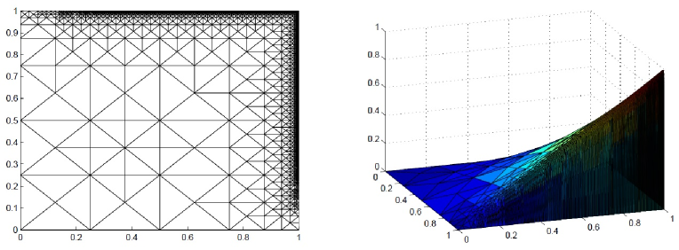
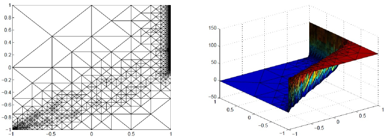
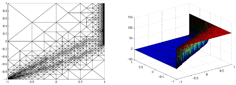
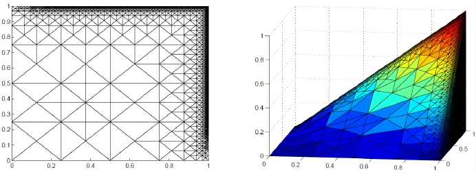
Figure 2: An adaptive mesh with 54855 triangles (left) and the approximation of displacement (piecewise linear element) on the corresponding mesh (right) for ε=1012𝜀superscript1012\varepsilon=10^{-12} by using the estimator from (3.3).
Refer to caption
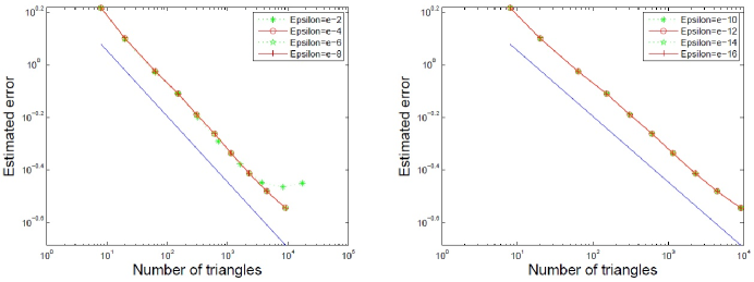
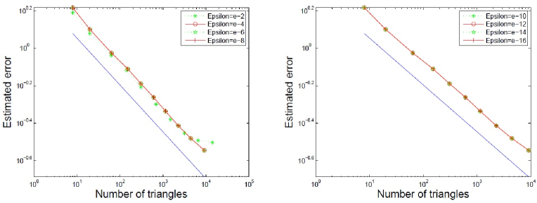
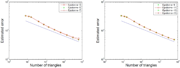
Figure 3: Estimated error of the flux against the number of elements in adaptively refined meshes for ε𝜀\varepsilon from 102superscript10210^{-2} to 108superscript10810^{-8} (left) and from 1010superscript101010^{-10} to 1016superscript101610^{-16} (right) by using the estimator from (3.3).
Refer to caption
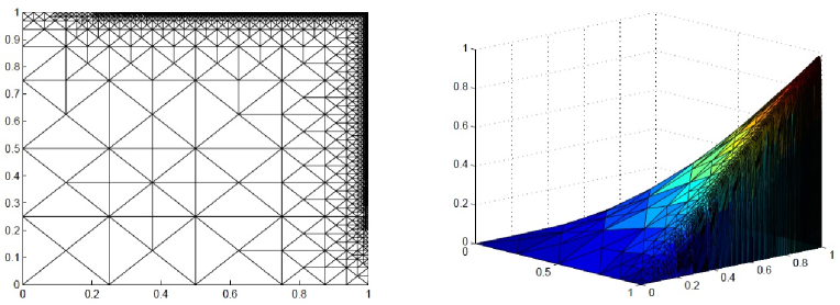
Figure 4: An adaptive mesh with 30869 triangles (left) and the approximation of displacement (piecewise linear element) on the corresponding mesh (right) for ε=1016𝜀superscript1016\varepsilon=10^{-16} by using the estimator from (3.2).
Refer to caption
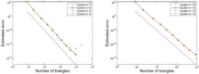
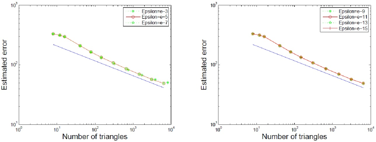
Figure 5: Estimated error of the flux against the number of elements in adaptively refined meshes for ε𝜀\varepsilon from 102superscript10210^{-2} to 108superscript10810^{-8} (left) and from 1010superscript101010^{-10} to 1016superscript101610^{-16} (right) by using the estimator from (3.2).
Refer to caption
Figure 6: An adaptive mesh with 17382 triangles (left) and the approximation of displacement (piecewise linear element) on the corresponding mesh (right) for ε=1016𝜀superscript1016\varepsilon=10^{-16} by using the estimator from (6.1).
Refer to caption
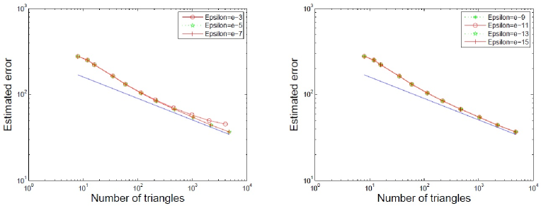
Figure 7: Estimated error of the flux against the number of elements in adaptively refined meshes for ε𝜀\varepsilon from 102superscript10210^{-2} to 108superscript10810^{-8} (left) and from 1010superscript101010^{-10} to 1016superscript101610^{-16} (right) by using the estimator from (6.1).
Refer to caption
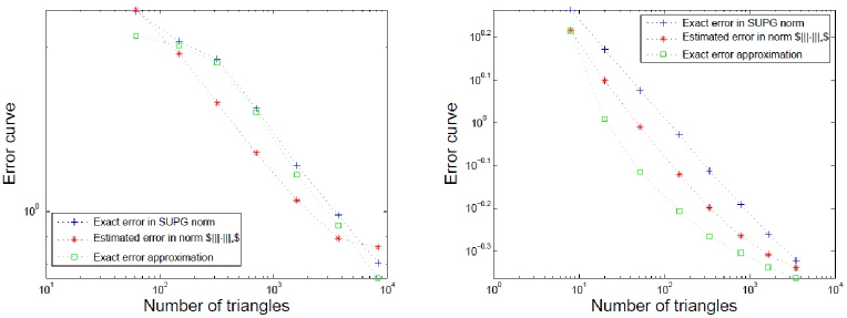
Figure 8: Exact error in SUPG norm, estimated error in norm |||||||||\cdot|||_{*}, and exact error approximation in norm ||||||ε|||\cdot|||_{\varepsilon} for explicit recovering for Example 1 with θ=0.5𝜃0.5\theta=0.5, ε=102𝜀superscript102\varepsilon=10^{-2}, and δK=16hKsubscript𝛿𝐾16subscript𝐾\delta_{K}=16h_{K} (left), and θ=0.5𝜃0.5\theta=0.5, ε=106𝜀superscript106\varepsilon=10^{-6}, and δK=4hKsubscript𝛿𝐾4subscript𝐾\delta_{K}=4h_{K} (right).

In Figures 2, 5, and 8, we plot adaptive meshes and numerical displacements by using the estimators obtained from the explicit recovery (3.3), the L2superscript𝐿2L^{2}-projection recovery (3.2), and the H(div)𝐻divH({\rm div}) recovery (6.1), respectively. Here the stabilization parameter is chosen as δK=hKsubscript𝛿𝐾subscript𝐾\delta_{K}=h_{K} on each element K𝒯h𝐾subscript𝒯K\in\mathcal{T}_{h}. Note that the constant C𝐶C in the stabilization parameter γKsubscript𝛾𝐾\gamma_{K} in H(div)𝐻divH({\rm div}) recovery (6.1) is taken as C=1𝐶1C=1 throughout numerical experiments.

It is observed that strong mesh refinements occur along x=1𝑥1x=1 and y=1𝑦1y=1, where the estimators correctly capture boundary layers and resolve them in convection-dominated regimes. Figures 3, 5, and 8, which are respectively in correspondence to (4.1), (4.2), and (6.5), report the estimated error against the number of elements in adaptively refined meshes obtained by using estimators from flux recoveries (3.3), (3.2), and (6.1), respectively. Here δK=16hKsubscript𝛿𝐾16subscript𝐾\delta_{K}=16h_{K}, the errors are measured in |||||||||\cdot|||_{*}, and ε𝜀\varepsilon is from 102superscript10210^{-2} to 1016superscript101610^{-16}. It is observed that the estimated errors depend on DOF𝐷𝑂𝐹DOF uniformly in ε𝜀\varepsilon. The estimators work well even if Péclet number is large, and the estimated errors of all three cases are convergent. As indicated in Remark 2.2, we substitute |uuh|subscriptnorm𝑢subscript𝑢|||u-u_{h}|||_{*} with uuhSUPGsubscriptnorm𝑢subscript𝑢SUPG||u-u_{h}||_{\rm SUPG} or |uuh|εsubscriptnorm𝑢subscript𝑢𝜀|||u-u_{h}|||_{\varepsilon} to compute the effectivity indices. We point out that the performance of the true error |uuh|subscriptnorm𝑢subscript𝑢|||u-u_{h}|||_{*} is between that of |uuh|εsubscriptnorm𝑢subscript𝑢𝜀|||u-u_{h}|||_{\varepsilon} and uuhSUPGsubscriptnorm𝑢subscript𝑢SUPG||u-u_{h}||_{{\rm SUPG}} up to a multiple of a constant independent of hh and ε𝜀\varepsilon. To confirm this assertion, Figure 8 illustrates uuhSUPGsubscriptnorm𝑢subscript𝑢SUPG||u-u_{h}||_{{\rm SUPG}}, the estimated error, and |uuh|εsubscriptnorm𝑢subscript𝑢𝜀|||u-u_{h}|||_{\varepsilon}. It is observed that, in the convection-dominated regime, the behavior of the true error is very similar to that of |uuh|εsubscriptnorm𝑢subscript𝑢𝜀|||u-u_{h}|||_{\varepsilon} and uuhSUPGsubscriptnorm𝑢subscript𝑢SUPG||u-u_{h}||_{{\rm SUPG}}. Thus, it is reasonable to use |uuh|εsubscriptnorm𝑢subscript𝑢𝜀|||u-u_{h}|||_{\varepsilon} or uuhSUPGsubscriptnorm𝑢subscript𝑢SUPG||u-u_{h}||_{{\rm SUPG}} to approximate the true error |uuh|subscriptnorm𝑢subscript𝑢|||u-u_{h}|||_{*} when convection dominates. In Table 2, we show numerical results for implicit L2superscript𝐿2L^{2}-projection recovering for ε=106𝜀superscript106\varepsilon=10^{-6}, θ=0.5𝜃0.5\theta=0.5, and δK=4hKsubscript𝛿𝐾4subscript𝐾\delta_{K}=4h_{K}. The effectivity indices (ratio of estimated and exact errors) are close to 111 after 8 iterations. Moreover, the estimators are robust with respect to ε𝜀\varepsilon.

We have checked the cases for δKsubscript𝛿𝐾\delta_{K} from δK=hKsubscript𝛿𝐾subscript𝐾\delta_{K}=h_{K} to δK=16hKsubscript𝛿𝐾16subscript𝐾\delta_{K}=16h_{K}, and found that the choice of δKsubscript𝛿𝐾\delta_{K} has a slight influence to the quality of the mesh. This observation indicates that adaptivity and stabilization for convection-diffusion equation is worthy of further study. In fact, the current state-of-the-art in stabilization is not completely satisfactory. In particular, the choice of stabilization parameters is still a subtle issue that is not fully understood. This is reflected either by remaining unphysical oscillations in the numerical solution or by smearing solution features too much. For more discussion on this subject, we refer to [14].

Table 1: Example 1: k𝑘k – the number of iterations; ηksubscript𝜂𝑘\eta_{k} – the estimated numerical error in |||||||||\cdot|||_{*}; errSUPG𝑒𝑟subscript𝑟SUPGerr_{\rm SUPG} and eff-index1 – the exact error in ||||SUPG||\cdot||_{\rm SUPG} and the corresponding effectivity index; and errAPP𝑒𝑟subscript𝑟APPerr_{\rm APP} and eff-index2 – the exact approximation error in ||||||ε|||\cdot|||_{\varepsilon} and the corresponding effectivity index. Here ε=106𝜀superscript106\varepsilon=10^{-6}, θ=0.5𝜃0.5\theta=0.5, and δK=4hKsubscript𝛿𝐾4subscript𝐾\delta_{K}=4h_{K}.
k𝑘k 111 222 333 444 555 666 777 888
ηksubscript𝜂𝑘\eta_{k} 1.6476 1.2551 0.9790 0.7580 0.6328 0.5438 0.4908 0.4573
errSUPG𝑒𝑟subscript𝑟SUPGerr_{\rm SUPG} 1.8419 1.4871 1.1914 0.9387 0.7717 0.6445 0.5492 0.4765
eff-index1 0.8945 0.8440 0.8217 0.8075 0.8200 0.8437 0.8936 0.9598
errAPP𝑒𝑟subscript𝑟APPerr_{\rm APP} 0.8204 0.6811 0.5760 0.4971 0.4519 0.4253 0.4018 0.3852
eff-index2 2.0083 1.8427 1.6998 1.5230 1.4002 1.2786 1.2216 1.1872
Table 2: Example 2: Numerical results by (3.3) with δK=16hKsubscript𝛿𝐾16subscript𝐾\delta_{K}=16h_{K} and θ=0.3𝜃0.3\theta=0.3. In the table, ε𝜀\varepsilon is the singular perturbation parameter, ηksubscript𝜂𝑘\eta_{k} is the estimated numerical error, TOL is the given tolerance, DOF is the degrees of freedom, hmax(ε)subscriptmax𝜀h_{\rm max}(\varepsilon) and hmin(ε)subscriptmin𝜀h_{\rm min}(\varepsilon) are respectively the largest and smallest mesh sizes, and k𝑘k is the number of iterations.
ε𝜀\varepsilon 106superscript10610^{-6} 105superscript10510^{-5} 104superscript10410^{-4} 103superscript10310^{-3} 102superscript10210^{-2}
ηksubscript𝜂𝑘\eta_{k}/TOL 24.159 29.5353 51.0934 86.1609 154.3741
DOF 28194 15696 1999 368 75
hmax(ε)subscriptmax𝜀h_{\rm max}(\varepsilon) 0.55902 0.55902 0.55902 0.55902 1.118034
hmin(ε)subscriptmin𝜀h_{\rm min}(\varepsilon) 7.63e-06 3.05e-05 4.88e-04 3.91e-03 0.031250
k𝑘k 20 18 14 11 8

7.2 Example 2: interior and boundary layer

This model problem is one of the examples solved by Verfürth in ALF software. Let Ω=(1,1)2Ωsuperscript112\Omega=(-1,1)^{2}. We set the velocity field 𝐚=(2,1)𝐚21{\bf a}=(2,1), the reaction coefficient b=0𝑏0b=0, and the source term f=0𝑓0f=0 in (1.1), and consider cases for ε𝜀\varepsilon from 103superscript10310^{-3} to 1015superscript101510^{-15}. The following Dirichlet boundary conditions are applied: u(x,y)=0𝑢𝑥𝑦0u(x,y)=0 along x=1𝑥1x=-1 and y=1𝑦1y=1, and u(x,y)=100𝑢𝑥𝑦100u(x,y)=100 along x=1𝑥1x=1 and y=1𝑦1y=-1. The exact solution of this problem is not available, which however exhibits an exponential boundary layer along the boundary {(x,y):x=1,y>0}conditional-set𝑥𝑦formulae-sequence𝑥1𝑦0\{(x,y)\;:\>x=1,y>0\}, and a parabolic interior layer along the line segment connecting points (1,1)11(-1,-1) and (1,0)10(1,0). Note that the interior layer extends in the direction of the convection coefficient.
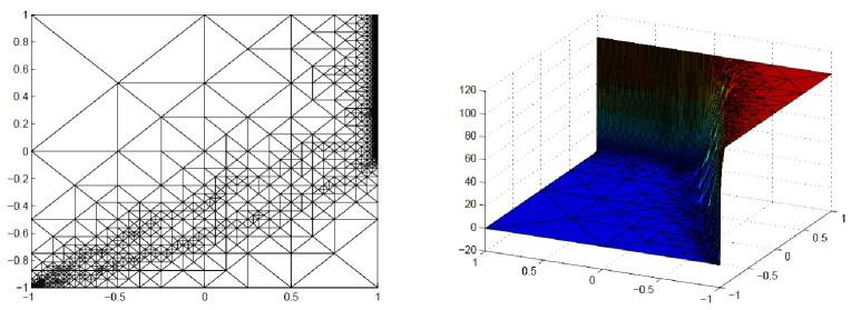
Refer to caption
Figure 9: An adaptive mesh with 14315 triangles (left) and the approximation of displacement (piecewise linear element) on the corresponding mesh (right) for ε=1011𝜀superscript1011\varepsilon=10^{-11} by using the estimator from (3.3).
Refer to caption
Figure 10: Estimated error of the flux against the number of elements in adaptively refined meshes for ε𝜀\varepsilon from 103superscript10310^{-3} to 107superscript10710^{-7} (left) and from 109superscript10910^{-9} to 1015superscript101510^{-15} (right) by using the estimator from (3.3).
Refer to caption
Figure 11: An adaptive mesh with 7761 triangles (left) and the approximation of displacement (piecewise linear element) on the corresponding mesh (right) for ε=1011𝜀superscript1011\varepsilon=10^{-11} by using the estimator from (3.2).
Refer to caption
Figure 12: Estimated error of the flux against the number of elements in adaptively refined meshes for ε𝜀\varepsilon from 103superscript10310^{-3} to 107superscript10710^{-7} (left) and from 109superscript10910^{-9} to 1015superscript101510^{-15} (right) by using the estimator from (3.2).
Refer to caption
Figure 13: An adaptive mesh with 27309 triangles (left) and the approximation of displacement (piecewise linear element) on the corresponding mesh (right) for ε=1011𝜀superscript1011\varepsilon=10^{-11} by using the estimator from (6.1).
Refer to caption
Figure 14: Estimated error of the flux against the number of elements in adaptively refined meshes for ε𝜀\varepsilon from 103superscript10310^{-3} to 107superscript10710^{-7} (left) and from 109superscript10910^{-9} to 1015superscript101510^{-15} (right) by using the estimator from (6.1).

We choose the same initial mesh as in Example 1. From Figures 10, 12, and 14, which are respectively depicted by using the estimators obtained from the explicit recovery (3.3), the L2superscript𝐿2L^{2}-projection recovery (3.2), and the H(div)𝐻divH({\rm div}) recovery (6.1), and by choosing the stabilization parameters as δK=hKsubscript𝛿𝐾subscript𝐾\delta_{K}=h_{K}. It is observed that the meshes are refined in both the exponential and the parabolic layer regions, but the refinement first occurs in the region near {(x,y):x=1,y>0}conditional-set𝑥𝑦formulae-sequence𝑥1𝑦0\{(x,y)\;:\>x=1,y>0\}. The reason is that the exponential layer is much stronger than the parabolic layer. It is also observed that each one of three estimators capture the behavior of the solution pretty well, even when the singular perturbation parameter ε𝜀\varepsilon is very small.

Figures 10, 12, and 14 are depicted by using the estimators obtained from the flux recovery (3.3), (3.2), and (6.1), respectively, and by choosing the stabilization parameters as δK=16hKsubscript𝛿𝐾16subscript𝐾\delta_{K}=16h_{K}. The estimated error against the number of elements in adaptively refined mesh for ε𝜀\varepsilon from 103superscript10310^{-3} to 1015superscript101510^{-15} are reported. It is observed that all three estimated errors from respective estimators in norm |||||||||\cdot|||_{*} reduce uniformly in sufficiently small ε𝜀\varepsilon in absence of reaction term. In addition, the same convergence rates as in Example 1 are obtained. It is also noticed that the performance of the three estimators are similar.

In Table 2, data for different ε𝜀\varepsilons are provided. The adaptive iterations refine elements till the layer is resolved or the TOL is met. One may observe that the performance of the error estimators depends on the TOL; the minimum mesh sizes hminsubscript𝑚𝑖𝑛h_{min} are of order O(εhmax)𝑂𝜀subscript𝑚𝑎𝑥O(\varepsilon h_{max}) or O(ε)𝑂𝜀O(\varepsilon), since the maximum mesh sizes hmax(ε)subscript𝑚𝑎𝑥𝜀h_{max}(\varepsilon) and the initial mesh size h0subscript0h_{0} are of similar sizes; the DOF required for resolving layers will increase when TOL and/or ε𝜀\varepsilon decrease; and the proposed error estimators are robust with respect to ε𝜀\varepsilon. On the other hand, due to the current state-of-the-art in stabilization, spurious oscillations may occur on very fine mesh, which will hence affect the quality of mesh refinement of further iterations and the rate of convergence of the method; cf. [14] and the plots for ε=102𝜀superscript102\varepsilon=10^{-2} in Figures 3 and 5.

References

  • [1] R.A. Adams, Sobolev space, Academic Press, New York. 1975.
  • [2] M. Ainsworth, A. Allends, G. R. Barrenechea, and R. Rankin, Fully computable a posteriori error bounds for stabilized FEM approximations of convection-reaction-diffusion problems in three dimentions, Int. J. Numer. Meth. Fluids, 73 (2013), no. 9, 765–790.
  • [3] M. Ainsworth and A.W. Craig, A posteriori error estimation in finite element method, Numer. Math., 36 (1991), 429–463.
  • [4] M. Ainsworth and J.T. Oden, A posteriori error estimation in finite element analysis, Pure Appl. Math., Wiley-Interscience, John Wiley &\& Sons, New York, 2000.
  • [5] M. Augustin, A. Caiazzo, A. Fiebach, J. Fuhrmann, V. Jhon, A. Linke, and R. Umla, An assessment of discretizations for convection-dominated convection-diffusion equations, Comput. Methods Appl. Mech. Engrg., 200 (2011), 3395-3409.
  • [6] R. Bank and J. Xu, Asymptotically exact a posteriori error estimators, Part 1: Grids with superconvergence, SIAM J. Numer. Anal., 41 (2003), 2294–2312; Part 2: General unstructured grids, SIAM J. Numer. Anal., 41 (2003), 2313–2332.
  • [7] R. Bank, J. Xu, and B. Zheng, Superconvergent derivative recovery for Lagrange triangular elmements of degree p𝑝p on unstructured grids, SIAM J. Numer. Anal., 45 (2007), 2032–2046.
  • [8] S. Berron, Robustness in a posteriori error analysis for FEM flow models, Numer. Math. 91 (2002), no. 3, 389–422.
  • [9] Z. Cai and S. Zhang, Recovery-based error estimator for interface problems: conforming linear elemnts, SIAM J. Numer. Anal., 47 (2009), no. 3, 2132–2156.
  • [10] Z. Cai and S. Zhang, Flux recovery and a posteriori error estimators: conforming elements for scalar elliptic equations, SIAM J. Numer. Anal., 48 (2010), no. 2, 578–602.
  • [11] C. Carstensen, All first-order averaging technique for a posteriori finite element error control on unstructure grids are efficient and reliable, Math. Comp., 73 (2003), 1153–1165.
  • [12] P.G. Ciarlet, The finite element method for elliptic problems, Nort-Holland, Amsterdam, 1978.
  • [13] P. Clemént, Approximation by finite element functions using local regularization, RAIRO Sér. Rouge Anal. Numér., 2 (1975), 77–84.
  • [14] A. Cohen, W. Dahmen, and G. Welper, Adaptivity and variational stablization for convection-diffusion equations, ESAIM: Mathematical Modelling and Numerical Analysis, 46 (2012), no. 5, 1247–1273
  • [15] S.H. Du and Z. Zhang, A robust residual-type a posteriori error estimator for convection-diffusion equations, Journal of Scientific Computing, 65 (2015), pp. 138-170.
  • [16] L.P. Franca, S.L. Frey, and T.J.R. Hughes, Stabilized finite element methods I: Application to the advective-diffusive model, Comput. Methods Appl. Mech. Engrg., 95 (1992), 253–276.
  • [17] T.J.R. Hughes and A. Brooks, Streamline upwind/Petrov Garlerkin formulations for the convection dominated flows with particular emphasis on the incompressible Navier-Stokes equations, Comput. Methods Appl. Mech. Engrg., 54 (1982), 199–259.
  • [18] V. John and J. Novo, A robust SUPG norm a posteriori error estimator for stationary convection-diffusion equations, Comput. Meth. Appl. Mech. Engrg., 255 (2013), 289–305.
  • [19] G. Kunert, A posteriori error estimation for convection dominated problems on anisotropic meshes, Math. Methods Appl. Sci. 26 (2003), no. 7, 589–617.
  • [20] J.S. Ovall, Fixing a “bug” in recovery-type a posteriori error estimators, Technical report 25, Max-Planck-Institute fur Mathematick in den Naturwissenschaften, Bonn, Germany, 2006.
  • [21] J.S. Ovall, Two dangers to avoid when using gradient recovery methods for finite element error estimation and adaptivity, Technical report 6, Max-Planck-Institute fur Mathematick in den Naturwissenschaften, Bonn, Germany, 2006.
  • [22] G. Rapin and G. Lube, A stabilized scheme for the Lagrange multiplier method for advection-diffusion equations, Math. Models Methods Appl. Sci. 14 (2004), no. 7, 1035–1060.
  • [23] H.G. Roos, M. Stynes, and L. Tobiska, Robust numerical methods for singularly perturbed differential equations, Springer-Verlag Berlin Heidelberg, 2008.
  • [24] G. Sangalli, A robust a posteriori estimator for the residual free bubbles method applied to advection-dominated problems, Numer. Math., 89 (2001), 379–399.
  • [25] G. Sangalli, Robust a-posteriori estimator for advection-diffusion-reaction problems, Math. Comp., 77 (2008), no. 261, 41–70.
  • [26] L. Tobiska and R. Verfürth, Robust a-posteriori error estimates for stablized finite element methods, IMA J Numer. Anal., (2015), doi: 10.1093//imanum//dru060.
  • [27] R. Verfürth, A posteriori error estimators for convection-diffusion equations, Numer. Math., 80 (1998), 641–663.
  • [28] R. Verfürth, Robust a posteriori error estimates for stationary convection-diffusion equations, SIAM J.Numer. Anal., 43 (2005), 1766–1782.
  • [29] M. F. Wheeler and I. Yotov, A multipoint flux mixed finite element method, SIAM J. Numer. Anal., 44 (2006), 2082–2106.
  • [30] Z. Zhang, A posteriori error estimates on irregular grids based on gradient recovery, Adv. Comput. Math., 15 (2001), 363–374.
  • [31] Z. Zhang, Recovery techniques in finite element methods, in Adaptive Computations: Theory and Algorithms, Mathematics Monogr. Ser. 6, T. Tang and J. Xu, eds., Science Publisher, New York, 333–412, 2007.
  • [32] O.C. Zienkiewicz and J.Z. Zhu, A simple error estimator and adaptive procedure for practical engineering analysis, Internat. J. Numer. Methods Engrg., 24 (1987), 337–357.
  • [33] O.C. Zienkiewicz and J.Z. Zhu, The superconvergent patch recovery and a posteriori error estimates, Part 1: The recovery technique, Internat. J. Numer. Methods Engrg., 33 (1992), 1331–1364; Part 2: Error estimates and adaptivity, Internat. J. Numer. Methods Engrg., 33 (1992), 1365–1382.