Learning Robust Features for Gait Recognition by Maximum Margin Criterion

Abstract

In the field of gait recognition from motion capture data, designing human-interpretable gait features is a common practice of many fellow researchers. To refrain from ad-hoc schemes and to find maximally discriminative features we may need to explore beyond the limits of human interpretability. This paper contributes to the state-of-the-art with a machine learning approach for extracting robust gait features directly from raw joint coordinates. The features are learned by a modification of Linear Discriminant Analysis with Maximum Margin Criterion so that the identities are maximally separated and, in combination with an appropriate classifier, used for gait recognition. Experiments on the CMU MoCap database show that this method outperforms eight other relevant methods in terms of the distribution of biometric templates in respective feature spaces expressed in four class separability coefficients. Additional experiments indicate that this method is a leading concept for rank-based classifier systems.

I Introduction

From the surveillance perspective, gait pattern biometrics is appealing for its possibility of being performed at a distance and without body-invasive equipment or subject’s cooperation. This allows data acquisition without a subject’s consent. As the data are collected with high participation rate and surveilled subjects are not expected to claim their identities, the trait is preferably employed for identification rather than for authentication.

Motion capture technology provides video clips of walking individuals containing structural motion data. The format keeps an overall structure of the human body and holds estimated 3D positions of major anatomical landmarks as the person moves. These so-called motion capture data (MoCap) can be collected online by a system of multiple cameras (Vicon) or a depth camera (Microsoft Kinect). To visualize motion capture data (see Figure 1), a simplified stick figure representing the human skeleton (a graph of joints connected by bones) can be recovered from the values of body point spatial coordinates. With recent rapid improvement in MoCap sensor accuracy, we believe in an affordable MoCap technology that can be installed in the streets and identify people from MoCap data.

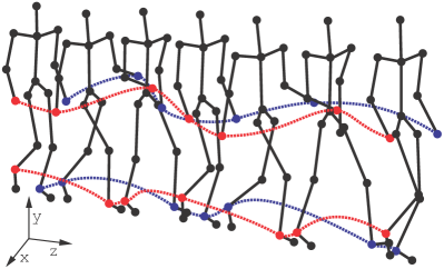
Figure 1: Motion capture data. Skeleton is represented by a stick figure of 31 joints (only 17 are drawn here). Seven selected video frames of a walk sequence contain 3D coordinates of each joint in time. The red and blue lines track trajectories of hands and feet. [1]

Primary goal of this work is to project a method for learning robust gait features from raw MoCap data. A collection of extracted features builds a gait template that serves as the walker’s signature. Templates are stored in a central database. Recognition of a person involves capturing their walk sample, extracting gait features to compose a template, and finally querying this database for a set of similar templates to report the most likely identity. Similarity of two templates is expressed in a single number computed by a similarity/distance function.

Many geometric gait features have been introduced over the past few years: Ahmed et al. [2] extract horizontal and vertical distances of selected joint pairs. Andersson et al. [3] calculate mean and standard deviation in the signals of lower joint (hips, knees and ankles) angles. Ball et al. [4] select mean, standard deviation and maximum of the signals of lower joint (hips, knees and ankles) angles. Dikovski et al. [5] construct 7 different feature sets from a broad spectrum of geometric features, such as static body parameters, joint angles and inter-joint distances aggregated within a gait cycle, along with various statistics. Kwolek et al. [6] extract bone rotations, inter-joint distances, and the person’s height. Preis et al. [7] define thirteen pose attributes, eleven of them static body parameters and the other two dynamic parameters: step length and walk speed. Sinha et al. [8] combine a number of gait features: areas of upper and lower body, inter-joint distances and all features introduced by Ball et al. [4] and Preis et al. [7]. Clearly, joint angles and step length are schematic and human-interpretable, which is convenient for visualizations and for intuitive understanding of the models, but unnecessary for automatic gait recognition. This application prefers learning features that maximally separate the identities and are not limited by such dispensable factors. Section II gives a scheme for learning the features by Maximum Margin Criterion.

We have implemented and evaluated all methods on a testing database described in Section III-A. Their performance is expressed in several evaluation metrics defined in Section III-B. Results are presented and discussed in Section III-C.

II Learning Gait Features

In statistical pattern recognition, reducing space dimensionality is a common technique to overcome class estimation problems. Classes are discriminated by projecting high-dimensional input data onto low-dimensional sub-spaces by linear transformations with the goal of maximizing the class separability. We are interested in finding an optimal feature space where a gait template is close to those of the same walker and far from those of different walkers.

Let the model of a human body have $J$ joints and all samples be linearly normalized to their average length $T$. Labeled learning data in a sample (measurement) space have the form ${\mathcal{G}}_{L}=\left\{\left(\mathbf{g}_{n},\ell_{n}\right)\right\}_{n=1}^{{N}_{L}}$ where

$$\mathbf{g}_{n}=\left[[\gamma_{1}\left(1\right)\,\cdots\,\gamma_{J}\left(1\right)]^{\top}\,\cdots\,[\gamma_{1}\left(T\right)\,\cdots\,\gamma_{J}\left(T\right)]^{\top}\right]^{\top}$$ (1)

is a gait sample (one gait cycle) in which $\gamma_{j}\left(t\right)\in\mathbb{R}^{3}$ are 3D spatial coordinates of a joint $j\in\left\{1,\ldots,J\right\}$ at time $t\in\left\{1,\ldots,T\right\}$ normalized with respect to the person’s position and walk direction. See that ${\mathcal{G}}_{L}$ has dimensionality $D=3JT$. Each learning sample falls strictly into one of the learning identity classes $\left\{\mathcal{I}_{c}\right\}_{c=1}^{C}$. A class $\mathcal{I}_{c}$ has $N_{c}$ samples. Here $\mathcal{I}_{c}\cap\mathcal{I}_{c^{\prime}}=\emptyset$ for $c\neq c^{\prime}$ and ${\mathcal{G}}_{L}=\bigcup_{c=1}^{C}\mathcal{I}_{c}$. $\ell_{n}$ is the ground-truth label of the walker’s identity class. We say that samples $\mathbf{g}_{n}$ and $\mathbf{g}_{n^{\prime}}$ share a common walker if they are in the same class, i.e., $\mathbf{g}_{n},\mathbf{g}_{n^{\prime}}\in\mathcal{I}_{c}\Leftrightarrow\ell_{n}=\ell_{n^{\prime}}$.

We measure class separability of a given feature space by a representation of the Maximum Margin Criterion (MMC) used by the Vapnik’s Support Vector Machines (SVM) [9]

$$\mathcal{J}=\frac{1}{2}\sum_{c,c^{\prime}=1}^{C}\left(\left(\mu_{c}-\mu_{c^{\prime}}\right)^{\top}\left(\mu_{c}-\mu_{c^{\prime}}\right)-\operatorname{tr}\left(\mathbf{\Sigma}_{c}+\mathbf{\Sigma}_{c^{\prime}}\right)\right)$$ (2)

which is actually a summation of $\frac{1}{2}C(C-1)$ between-class margins. The margin is defined as the Euclidean distance of class means minus both individual variances (traces of scatter matrices $\mathbf{\Sigma}_{c}=\frac{1}{N_{c}}\sum_{n=1}^{N_{c}}\left(\mathbf{g}_{n}^{(c)}-\mu_{c}\right)\left(\mathbf{g}_{n}^{(c)}-\mu_{c}\right)^{\top}$ and similarly for $\mathbf{\Sigma}_{c^{\prime}}$). For the whole labeled data, we denote the between- and within-class and total scatter matrices

$$\begin{split}\mathbf{\Sigma}_{\mathrm{B}}&=\sum_{c=1}^{{C}_{L}}\left(\mu_{c}-\mu\right)\left(\mu_{c}-\mu\right)^{\top}\\ \mathbf{\Sigma}_{\mathrm{W}}&=\sum_{c=1}^{{C}_{L}}\frac{1}{N_{c}}\sum_{n=1}^{N_{c}}\left(\mathbf{g}_{n}^{(c)}-\mu_{c}\right)\left(\mathbf{g}_{n}^{(c)}-\mu_{c}\right)^{\top}\\ \mathbf{\Sigma}_{\mathrm{T}}&=\sum_{c=1}^{{C}_{L}}\frac{1}{N_{c}}\sum_{n=1}^{N_{c}}\left(\mathbf{g}_{n}^{(c)}-\mu\right)\left(\mathbf{g}_{n}^{(c)}-\mu\right)^{\top}=\mathbf{\Sigma}_{\mathrm{B}}+\mathbf{\Sigma}_{\mathrm{W}}\end{split}$$ (3)

where $\mathbf{g}_{n}^{(c)}$ denotes the $n$-th sample in class $\mathcal{I}_{c}$ and $\mu_{c}$ and $\mu$ are sample means for class $\mathcal{I}_{c}$ and the whole data set, respectively, that is, $\mu_{c}=\frac{1}{N_{c}}\sum_{n=1}^{N_{c}}\mathbf{g}_{n}^{(c)}$ and $\mu=\frac{1}{{N}_{L}}\sum_{n=1}^{{N}_{L}}\mathbf{g}_{n}$. Now we obtain

$$\begin{split}\mathcal{J}&\!=\!\frac{1}{2}\sum_{c,c^{\prime}=1}^{C}\left(\mu_{c}-\mu_{c^{\prime}}\right)^{\top}\left(\mu_{c}-\mu_{c^{\prime}}\right)-\frac{1}{2}\sum_{c,c^{\prime}=1}^{C}\operatorname{tr}\left(\mathbf{\Sigma}_{c}+\mathbf{\Sigma}_{c^{\prime}}\right)\\ &\!=\!\frac{1}{2}\sum_{c,c^{\prime}=1}^{C}\left(\mu_{c}-\mu+\mu-\mu_{c^{\prime}}\right)^{\top}\left(\mu_{c}-\mu+\mu-\mu_{c^{\prime}}\right)-\sum_{c=1}^{C}\operatorname{tr}\left(\mathbf{\Sigma}_{c}\right)\\ &\!=\!\operatorname{tr}\left(\sum_{c=1}^{C}\left(\mu_{c}-\mu\right)\left(\mu_{c}-\mu\right)^{\top}\right)-\operatorname{tr}\left(\sum_{c=1}^{C}\mathbf{\Sigma}_{c}\right)\\ &\!=\!\operatorname{tr}\left(\mathbf{\Sigma}_{\mathrm{B}}\right)-\operatorname{tr}\left(\mathbf{\Sigma}_{\mathrm{W}}\right)=\operatorname{tr}\left(\mathbf{\Sigma}_{\mathrm{B}}-\mathbf{\Sigma}_{\mathrm{W}}\right).\end{split}$$ (4)

Since $\operatorname{tr}\left(\mathbf{\Sigma}_{\mathrm{B}}\right)$ measures the overall variance of the class mean vectors, a large one implies that the class mean vectors scatter in a large space. On the other hand, a small $\operatorname{tr}\left(\mathbf{\Sigma}_{\mathrm{W}}\right)$ implies that classes have a small spread. Thus, a large $\mathcal{J}$ indicates that samples are close to each other if they share a common walker but are far from each other if they are performed by different walkers. Extracting features, that is, transforming the input data in the measurement space into a feature space of higher $\mathcal{J}$, can be used to link new observations of walkers more successfully.

Feature extraction is given by a linear transformation (feature) matrix $\mathbf{\Phi}\in\mathbb{R}^{D\times\widehat{D}}$ from a $D$-dimensional measurement space $\mathcal{G}=\left\{\mathbf{g}_{n}\right\}_{n=1}^{N}$ of not necessarily labeled gait samples into a $\widehat{D}$-dimensional feature space $\widehat{\mathcal{G}}=\left\{\widehat{\mathbf{g}}_{n}\right\}_{n=1}^{N}$ of gait templates where $\widehat{D}<D$. Gait samples $\mathbf{g}_{n}$ are transformed into gait templates $\widehat{\mathbf{g}}_{n}=\mathbf{\Phi}^{\top}\mathbf{g}_{n}$. The objective is to learn a transform $\mathbf{\Phi}$ that maximizes the accumulated margin of the feature space

$$\mathcal{J}\left(\mathbf{\Phi}\right)=\operatorname{tr}\left(\mathbf{\Phi}^{\top}\left(\mathbf{\Sigma}_{\mathrm{B}}-\mathbf{\Sigma}_{\mathrm{W}}\right)\mathbf{\Phi}\right).$$ (5)

Once the transformation is found, all measured samples are transformed into templates (in the feature space) along with the class means and covariances. The templates are compared by the Mahalanobis distance function

$$\widehat{\delta}\left(\widehat{\mathbf{g}}_{n},\widehat{\mathbf{g}}_{n^{\prime}}\right)=\sqrt{\left(\widehat{\mathbf{g}}_{n}-\widehat{\mathbf{g}}_{n^{\prime}}\right)^{\top}\mathbf{\widehat{\Sigma}}_{\mathrm{T}}^{-1}\left(\widehat{\mathbf{g}}_{n}-\widehat{\mathbf{g}}_{n^{\prime}}\right)}.$$ (6)

Now we show that solution to the optimization problem in Equation (5) can be obtained by eigendecomposition of the matrix $\mathbf{\Sigma}_{\mathrm{B}}-\mathbf{\Sigma}_{\mathrm{W}}$. An important property to notice about the objective $\mathcal{J}\left(\mathbf{\Phi}\right)$ is that it is invariant w.r.t. rescalings $\mathbf{\Phi}\rightarrow\alpha\mathbf{\Phi}$. Since it is a scalar itself, we can always choose $\mathbf{\Phi}=\mathbf{f}_{1}\|\cdots\|\mathbf{f}_{\widehat{D}}$ such that $\mathbf{f}_{\widehat{d}}^{\top}\mathbf{f}_{\widehat{d}}=1$ and reduce the problem of maximizing $\mathcal{J}\left(\mathbf{\Phi}\right)$ into the constrained optimization problem

$$\begin{split}\max&\quad\sum_{\widehat{d}=1}^{\widehat{D}}\mathbf{f}_{\widehat{d}}^{\top}\left(\mathbf{\Sigma}_{\mathrm{B}}-\mathbf{\Sigma}_{\mathrm{W}}\right)\mathbf{f}_{\widehat{d}}\\ \mathrm{subject\,to}&\quad\mathbf{f}_{\widehat{d}}^{\top}\mathbf{f}_{\widehat{d}}-1=0\qquad\forall\widehat{d}=1,\ldots,\widehat{D}.\end{split}$$ (7)

To solve the above optimization problem, let us consider the Lagrangian

$$\mathcal{L}\left(\mathbf{f}_{\widehat{d}},\lambda_{\widehat{d}}\right)=\sum_{\widehat{d}=1}^{\widehat{D}}\mathbf{f}_{\widehat{d}}^{\top}\left(\mathbf{\Sigma}_{\mathrm{B}}-\mathbf{\Sigma}_{\mathrm{W}}\right)\mathbf{f}_{\widehat{d}}-\lambda_{\widehat{d}}\left(\mathbf{f}_{\widehat{d}}^{\top}\mathbf{f}_{\widehat{d}}-1\right)$$ (8)

with multipliers $\lambda_{\widehat{d}}$. To find the maximum, we derive it with respect to $\mathbf{f}_{\widehat{d}}$ and equate to zero

$$\frac{\partial\mathcal{L}\left(\mathbf{f}_{\widehat{d}},\lambda_{\widehat{d}}\right)}{\partial\mathbf{f}_{\widehat{d}}}=\left(\left(\mathbf{\Sigma}_{\mathrm{B}}-\mathbf{\Sigma}_{\mathrm{W}}\right)-\lambda_{\widehat{d}}\mathbf{I}\right)\mathbf{f}_{\widehat{d}}=0$$ (9)

which leads to

$$\left(\mathbf{\Sigma}_{\mathrm{B}}-\mathbf{\Sigma}_{\mathrm{W}}\right)\mathbf{f}_{\widehat{d}}=\lambda_{\widehat{d}}\mathbf{f}_{\widehat{d}}$$ (10)

where $\lambda_{\widehat{d}}$ are the eigenvalues of $\mathbf{\Sigma}_{\mathrm{B}}-\mathbf{\Sigma}_{\mathrm{W}}$ and $\mathbf{f}_{\widehat{d}}$ are the corresponding eigenvectors. Therefore,

$$\mathcal{J}\left(\mathbf{\Phi}\right)=\operatorname{tr}\left(\mathbf{\Phi}^{\top}\left(\mathbf{\Sigma}_{\mathrm{B}}-\mathbf{\Sigma}_{\mathrm{W}}\right)\mathbf{\Phi}\right)=\operatorname{tr}\left(\mathbf{\Phi}^{\top}\mathbf{\Lambda}\mathbf{\Phi}\right)=\operatorname{tr}\left(\mathbf{\Lambda}\right)$$ (11)

is maximized when $\mathbf{\Lambda}=\operatorname{diag}\left(\lambda_{1},\ldots,\lambda_{\widehat{D}}\right)$ has $\widehat{D}$ largest eigenvalues and $\mathbf{\Phi}$ contains the corresponding leading eigenvectors.

In the following we discuss how to calculate the eigenvectors of $\mathbf{\Sigma}_{\mathrm{B}}-\mathbf{\Sigma}_{\mathrm{W}}$ and to determine an optimal dimensionality $\widehat{D}$ of the feature space. First, we rewrite $\mathbf{\Sigma}_{\mathrm{B}}-\mathbf{\Sigma}_{\mathrm{W}}=2\mathbf{\Sigma}_{\mathrm{B}}-\mathbf{\Sigma}_{\mathrm{T}}$. Note that the null space of $\mathbf{\Sigma}_{\mathrm{T}}$ is a subspace of that of $\mathbf{\Sigma}_{\mathrm{B}}$ since the null space of $\mathbf{\Sigma}_{\mathrm{T}}$ is the common null space of $\mathbf{\Sigma}_{\mathrm{B}}$ and $\mathbf{\Sigma}_{\mathrm{W}}$. Thus, we can simultaneously diagonalize $\mathbf{\Sigma}_{\mathrm{B}}$ and $\mathbf{\Sigma}_{\mathrm{T}}$ to some $\mathbf{\Delta}$ and $\mathbf{I}$

$$\begin{split}\mathbf{\Psi}^{\top}\mathbf{\Sigma}_{\mathrm{B}}\mathbf{\Psi}&=\mathbf{\Delta}\\ \mathbf{\Psi}^{\top}\mathbf{\Sigma}_{\mathrm{T}}\mathbf{\Psi}&=\mathbf{I}\end{split}$$ (12)

with the $D\times\operatorname{rank}\left(\mathbf{\Sigma}_{\mathrm{T}}\right)$ eigenvector matrix

$$\mathbf{\Psi}=\mathbf{\Omega}\mathbf{\Theta}^{-\frac{1}{2}}\mathbf{\Xi}$$ (13)

where $\mathbf{\Omega}$ and $\mathbf{\Theta}$ are the eigenvector and eigenvalue matrices of $\mathbf{\Sigma}_{\mathrm{T}}$, respectively, and $\mathbf{\Xi}$ is the eigenvector matrix of $\mathbf{\Theta}^{-1/2}\mathbf{\Omega}^{\top}\mathbf{\Sigma}_{\mathrm{B}}\mathbf{\Omega}\mathbf{\Theta}^{-1/2}$. To calculate $\mathbf{\Psi}$, we use a fast two-step algorithm [10] in virtue of Singular Value Decomposition (SVD). SVD expresses a real $r\times s$ matrix $\mathbf{A}$ as a product $\mathbf{A}=\mathbf{U}\mathbf{D}\mathbf{V}^{\top}$ where $\mathbf{D}$ is a diagonal matrix with decreasing non-negative entries, and $\mathbf{U}$ and $\mathbf{V}$ are $r\times\min\left\{r,s\right\}$ and $s\times\min\left\{r,s\right\}$ eigenvector matrices of $\mathbf{A}\mathbf{A}^{\top}$ and $\mathbf{A}^{\top}\mathbf{A}$, respectively, and the non-vanishing entries of $\mathbf{D}$ are square roots of the non-zero corresponding eigenvalues of both $\mathbf{A}\mathbf{A}^{\top}$ and $\mathbf{A}^{\top}\mathbf{A}$. See that $\mathbf{\Sigma}_{\mathrm{T}}$ and $\mathbf{\Sigma}_{\mathrm{B}}$ can be expressed in the forms

$$\begin{split}\mathbf{\Sigma}_{\mathrm{T}}=&\enskip\mathbf{X}\mathbf{X}^{\top}\enskip\mathrm{where}\enskip\mathbf{X}=\frac{1}{\sqrt{{N}_{L}}}\left[\left(\mathbf{g}_{1}-\mu\right)\cdots\left(\mathbf{g}_{{N}_{L}}-\mu\right)\right]\enskip\text{and}\\ \mathbf{\Sigma}_{\mathrm{B}}=&\enskip\mathbf{\Upsilon}\mathbf{\Upsilon}^{\top}\enskip\text{where}\enskip\mathbf{\Upsilon}=\left[\left(\mu_{1}-\mu\right)\cdots\left(\mu_{{C}_{L}}-\mu\right)\right],\end{split}$$ (14)

respectively. Hence, we can obtain the eigenvectors $\mathbf{\Omega}$ and the corresponding eigenvalues $\mathbf{\Theta}$ of $\mathbf{\Sigma}_{\mathrm{T}}$ through the SVD of $\mathbf{X}$ and analogically $\mathbf{\Xi}$ of $\mathbf{\Theta}^{-1/2}\mathbf{\Omega}^{\top}\mathbf{\Sigma}_{\mathrm{B}}\mathbf{\Omega}\mathbf{\Theta}^{-1/2}$ through the SVD of $\mathbf{\Theta}^{-1/2}\mathbf{\Omega}^{\top}\mathbf{\Upsilon}$. The columns of $\mathbf{\Psi}$ are clearly the eigenvectors of $2\mathbf{\Sigma}_{\mathrm{B}}-\mathbf{\Sigma}_{\mathrm{T}}$ with the corresponding eigenvalues $2\mathbf{\Delta}-\mathbf{I}$. Therefore, to constitute the transform $\mathbf{\Phi}$ by maximizing the MMC, we should choose the eigenvectors in $\mathbf{\Psi}$ that correspond to the eigenvalues of at least $\frac{1}{2}$ in $\mathbf{\Delta}$. Note that $\mathbf{\Delta}$ contains at most $\operatorname{rank}\left(\mathbf{\Sigma}_{\mathrm{B}}\right)=C-1$ positive eigenvalues.

We found inspiration in the Fisher’s Linear Discriminant Analysis (LDA) [11] that uses the Fisher’s criterion

$$\mathcal{J}\left(\mathbf{\Phi}_{\mathrm{LDA}}\right)=\operatorname{tr}\left(\frac{\mathbf{\Phi}_{\mathrm{LDA}}^{\top}\mathbf{\Sigma}_{\mathrm{B}}\mathbf{\Phi}_{\mathrm{LDA}}}{\mathbf{\Phi}_{\mathrm{LDA}}^{\top}\mathbf{\Sigma}_{\mathrm{W}}\mathbf{\Phi}_{\mathrm{LDA}}}\right).$$ (15)

However, since the rank of $\mathbf{\Sigma}_{\mathrm{W}}$ is at most ${N}_{L}-C$, it is a singular (non-invertible) matrix if ${N}_{L}$ is less than $D+C$, or, analogously might be unstable if ${N}_{L}\ll D$. Small sample size is a substantial difficulty as it is necessary to calculate $\mathbf{\Sigma}_{\mathrm{W}}^{-1}$. To alleviate this, the measured data can be first projected to a lower dimensional space using Principal Component Analysis (PCA), resulting in a two-stage PCA+LDA feature extraction technique [12]

$$\begin{split}\mathcal{J}\left(\mathbf{\Phi}_{\mathrm{PCA}}\right)=&\operatorname{tr}\left(\mathbf{\Phi}_{\mathrm{PCA}}^{\top}\mathbf{\Sigma}_{\mathrm{T}}\mathbf{\Phi}_{\mathrm{PCA}}\right)\\ \mathcal{J}\left(\mathbf{\Phi}_{\mathrm{LDA}}\right)=&\operatorname{tr}\left(\frac{\mathbf{\Phi}_{\mathrm{LDA}}^{\top}\mathbf{\Phi}_{\mathrm{PCA}}^{\top}\mathbf{\Sigma}_{\mathrm{B}}\mathbf{\Phi}_{\mathrm{PCA}}\mathbf{\Phi}_{\mathrm{LDA}}}{\mathbf{\Phi}_{\mathrm{LDA}}^{\top}\mathbf{\Phi}_{\mathrm{PCA}}^{\top}\mathbf{\Sigma}_{\mathrm{W}}\mathbf{\Phi}_{\mathrm{PCA}}\mathbf{\Phi}_{\mathrm{LDA}}}\right)\end{split}$$ (16)

and the final transform is $\mathbf{\Phi}=\mathbf{\Phi}_{\mathrm{PCA}}\mathbf{\Phi}_{\mathrm{LDA}}$. Given that there are $\overline{D}$ principal components, then regardless of the dimensionality $D$ there are at least $\overline{D}+1$ independent data points. Thus, if the $\overline{D}\times\overline{D}$ matrix $\mathbf{\Phi}_{\mathrm{PCA}}^{\top}\mathbf{\Sigma}_{\mathrm{W}}\mathbf{\Phi}_{\mathrm{PCA}}$ is estimated from ${N}_{L}-C$ independent observations and providing the $C\leq\overline{D}\leq{N}_{L}-C$, we can always invert $\mathbf{\Phi}_{\mathrm{PCA}}^{\top}\mathbf{\Sigma}_{\mathrm{W}}\mathbf{\Phi}_{\mathrm{PCA}}$ and this way obtain the LDA estimate. Note that this method is sub-optimal for multi-class problems [13] as PCA keeps at most ${N}_{L}-C$ principal components whereas at least ${N}_{L}-1$ of them are necessary in order not to lose information. PCA+LDA in this form has been used for silhouette-based (2D) gait recognition by Su et al. [14] and is included in our experiments with MoCap (3D).

On given labeled learning data ${\mathcal{G}}_{L}$, Algorithm 1 and Algorithm 2 provided below are efficient ways of learning the transforms $\mathbf{\Phi}$ for MMC and PCA+LDA, respectively.

Algorithm 1 LearnTransformationMatrixMMC$\left({\mathcal{G}}_{L}\right)$

1:split ${\mathcal{G}}_{L}=\left\{\left(\mathbf{g}_{n},\ell_{n}\right)\right\}_{n=1}^{{N}_{L}}$ into $\left\{\mathcal{I}_{c}\right\}_{c=1}^{{C}_{L}}$ of $N_{c}=\left|\mathcal{I}_{c}\right|$ samples

2:compute overall mean $\mu=\frac{1}{{N}_{L}}\sum_{n=1}^{{N}_{L}}\mathbf{g}_{n}$ and individual class means $\mu_{c}=\frac{1}{N_{c}}\sum_{n=1}^{N_{c}}\mathbf{g}_{n}^{(c)}$

3:compute $\mathbf{\Sigma}_{\mathrm{B}}=\sum_{c=1}^{{C}_{L}}\left(\mu_{c}-\mu\right)\left(\mu_{c}-\mu\right)^{\top}$

4:compute $\mathbf{X}=\frac{1}{\sqrt{{N}_{L}}}\left[\left(\mathbf{g}_{1}-\mu\right)\cdots\left(\mathbf{g}_{{N}_{L}}-\mu\right)\right]$

5:compute $\mathbf{\Upsilon}=\left[\left(\mu_{1}-\mu\right)\cdots\left(\mu_{{C}_{L}}-\mu\right)\right]$

6:compute eigenvectors $\mathbf{\Omega}$ and corresponding eigenvalues $\mathbf{\Theta}$
of $\mathbf{\Sigma}_{\mathrm{T}}$ through SVD of $\mathbf{X}$

7:compute eigenvectors $\mathbf{\Xi}$ of $\mathbf{\Theta}^{\nicefrac{{-1}}{{2}}}\mathbf{\Omega}^{\top}\mathbf{\Sigma}_{\mathrm{B}}\mathbf{\Omega}\mathbf{\Theta}^{\nicefrac{{-1}}{{2}}}$
through SVD of $\mathbf{\Theta}^{\nicefrac{{-1}}{{2}}}\mathbf{\Omega}^{\top}\mathbf{\Upsilon}$

8:compute eigenvectors $\mathbf{\Psi}=\mathbf{\Omega}\mathbf{\Theta}^{\nicefrac{{-1}}{{2}}}\mathbf{\Xi}$

9:compute eigenvalues $\mathbf{\Delta}=\mathbf{\Psi}^{\top}\mathbf{\Sigma}_{\mathrm{B}}\mathbf{\Psi}$

10:return transform $\mathbf{\Phi}$ as eigenvectors in $\mathbf{\Psi}$
that correspond to the eigenvalues of at least $\nicefrac{{1}}{{2}}$ in $\mathbf{\Delta}$

Algorithm 2 LearnTransformationMatrixPCALDA$\left({\mathcal{G}}_{L}\right)$

1:split ${\mathcal{G}}_{L}=\left\{\left(\mathbf{g}_{n},\ell_{n}\right)\right\}_{n=1}^{{N}_{L}}$ into $\left\{\mathcal{I}_{c}\right\}_{c=1}^{{C}_{L}}$ of $N_{c}=\left|\mathcal{I}_{c}\right|$ samples

2:compute overall mean $\mu=\frac{1}{{N}_{L}}\sum_{n=1}^{{N}_{L}}\mathbf{g}_{n}$ and individual class means $\mu_{c}=\frac{1}{N_{c}}\sum_{n=1}^{N_{c}}\mathbf{g}_{n}^{(c)}$

3:compute $\mathbf{\Sigma}_{\mathrm{B}}=\sum_{c=1}^{{C}_{L}}\left(\mu_{c}-\mu\right)\left(\mu_{c}-\mu\right)^{\top}$

4:compute $\mathbf{\Sigma}_{\mathrm{W}}=\sum_{c=1}^{{C}_{L}}\frac{1}{N_{c}}\sum_{n=1}^{N_{c}}\left(\mathbf{g}_{n}^{(c)}-\mu_{c}\right)\left(\mathbf{g}_{n}^{(c)}-\mu_{c}\right)^{\top}$

5:compute eigenvectors $\mathbf{\Phi}_{\mathrm{PCA}}$ of $\mathbf{\Sigma}_{\mathrm{T}}=\mathbf{\Sigma}_{\mathrm{B}}+\mathbf{\Sigma}_{\mathrm{W}}$
that correspond to $\overline{D}$ largest eigenvalues (we set $\overline{D}={C}_{L}$)

6:compute eigenvectors $\mathbf{\Phi}_{\mathrm{LDA}}$
of $(\mathbf{\Phi}_{\mathrm{PCA}}^{\top}\mathbf{\Sigma}_{\mathrm{W}}\mathbf{\Phi}_{\mathrm{PCA}})^{-1}(\mathbf{\Phi}_{\mathrm{PCA}}^{\top}\mathbf{\Sigma}_{\mathrm{B}}\mathbf{\Phi}_{\mathrm{PCA}})$

7:return transform $\mathbf{\Phi}=\mathbf{\Phi}_{\mathrm{PCA}}\mathbf{\Phi}_{\mathrm{LDA}}$

III Experimental Evaluation

III-A Database

For the evaluation purposes we have extracted a large number of samples from the general MoCap database from CMU [15] as a well-known and recognized database of structural human motion data. It contains numerous motion sequences, including a considerable number of gait sequences. Motions are recorded with an optical marker-based Vicon system. People wear a black jumpsuit and have 41 markers taped on. The tracking space of 30 m², surrounded by 12 cameras of sampling rate of 120 Hz in the height from 2 to 4 meters above ground, creates a video surveillance environment. Motion videos are triangulated to get highly accurate 3D data in the form of relative body point coordinates (with respect to the root joint) in each video frame and stored in the standard ASF/AMC data format. Each registered participant is assigned with their respective skeleton described in an ASF file. Motions in the AMC files store bone rotational data, which is interpreted as instructions about how the associated skeleton deforms over time.

To use the collected data in a fairly manner, a prototypical skeleton is constructed and used to represent bodies of all subjects, shrouding the unique skeleton parameters of individual walkers. Assuming that all walking subjects are physically identical disables a trivial skeleton check as a potentially unfair 100% classifier. Moreover, this is a skeleton-robust solution as all bone rotational data are linked with a fixed skeleton. To obtain realistic parameters, it is calculated as the mean of all skeletons in the provided ASF files.

3D joint coordinates are calculated using bone rotational data and the prototypical skeleton. One cannot directly use raw values of joint coordinates, as they refer to absolute positions in the tracking space, and not all potential methods are invariant to person’s position or walk direction. To ensure such invariance, the center of the coordinate system is moved to the position of root joint $\gamma_{\mathrm{root}}\left(t\right)=[0,0,0]^{\top}$ for each time $t$ and axes are adjusted to the walker’s perspective: the X axis is from right (negative) to left (positive), the Y axis is from down (negative) to up (positive), and the Z axis is from back (negative) to front (positive). In the AMC file structure notation it is achieved by zeroing the root translation and rotation (root 0 0 0 0 0 0) in all frames of all motion sequences.

Since the general motion database contains all motion types, we extracted a number of sub-motions that represent gait cycles. First, an exemplary gait cycle was identified, and clean gait cycles were then filtered out using the DTW distance over bone rotations. The similarity threshold was set high enough so that even the least similar sub-motion still semantically represents a gait cycle. Finally, subjects that contributed with less than 10 samples were excluded. The final database has 54 walking subjects that performed 3,843 samples in total, which makes an average of about 71 samples per subject.

III-B Performance Metrics

All results are estimated with nested cross-validation (see Figure 2) that involves two partial cross-validation loops. In the outer 3-fold cross-validation loop, ${N}_{L}$ labeled templates in one fold are used for learning the features and thus training the model. This model is frozen and ready to be evaluated for class separability coefficients on the remaining two folds of ${N}_{E}$ labeled templates. Both learning and evaluation sets contain templates of all $C$ identities. Evaluation of classification metrics advances to the inner 10-fold cross-validation loop taking one dis-labeled fold as a testing set and other nine labeled folds as gallery. Test templates are classified by the winner-takes-all strategy, in which a test template $\widehat{\mathbf{g}}^{\mathrm{test}}$ gets assigned with the label $\ell_{\operatorname{argmin}_{i}\widehat{\delta}\left(\widehat{\mathbf{g}}^{\mathrm{test}},\widehat{\mathbf{g}}_{i}^{\mathrm{gallery}}\right)}$ of the gallery’s closest identity class.

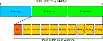
Figure 2: Nested cross-validation.

Correct Classification Rate (CCR) is often perceived as the ultimate qualitative measure; however, if a method has a low CCR, we cannot directly say if the system is failing because of bad features or a bad classifier. It is more explanatory to provide an evaluation in terms of class separability of the feature space. The class separability measures give an estimate on the recognition potential of the extracted features and do not reflect eventual combination with an unsuitable classifier:

• Davies-Bouldin Index: DBI

$$\mathrm{DBI}=\frac{1}{C}\sum_{c=1}^{C}\max\limits_{1\leq c^{\prime}\leq C,\,c^{\prime}\neq c}\frac{\sigma_{c}+\sigma_{c^{\prime}}}{\widehat{\delta}\left(\widehat{\mu}_{c},\widehat{\mu}_{c^{\prime}}\right)}$$ (17)

where $\sigma_{c}=\frac{1}{N_{c}}\sum_{n=1}^{N_{c}}\widehat{\delta}\left(\widehat{\mathbf{g}}_{n},\widehat{\mu}_{c}\right)$ is the average distance of all elements in identity class $\mathcal{I}_{c}$ to its centroid, and analogically for $\sigma_{c^{\prime}}$. Templates of low intra-class distances and of high inter-class distances have a low DBI.

• Dunn Index: DI

$$\mathrm{DI}=\frac{\min\limits_{1\leq c<c^{\prime}\leq C}\widehat{\delta}\left(\widehat{\mu}_{c},\widehat{\mu}_{c^{\prime}}\right)}{\max\limits_{1\leq c\leq C}\sigma_{c}}$$ (18)

with $\sigma_{c}$ from the above DBI. Since this criterion seeks classes with high intra-class similarity and low inter-class similarity, a high DI is more desirable.

• Silhouette Coefficient: SC

$$\mathrm{SC}=\frac{1}{{N}_{E}}\sum_{n=1}^{{N}_{E}}\frac{b(\widehat{\mathbf{g}}_{n})-a(\widehat{\mathbf{g}}_{n})}{\max\left\{a\left(\widehat{\mathbf{g}}_{n}),b(\widehat{\mathbf{g}}_{n}\right)\right\}}$$ (19)

where $a(\widehat{\mathbf{g}}_{n})=\frac{1}{N_{c}}\sum_{n^{\prime}=1}^{N_{c}}\widehat{\delta}\left(\widehat{\mathbf{g}}_{n},\widehat{\mathbf{g}}_{n^{\prime}}\right)$ is the average distance from $\widehat{\mathbf{g}}_{n}$ to other samples within the same identity class and $b(\widehat{\mathbf{g}}_{n})=\min\limits_{1\leq c^{\prime}\leq C,\,c^{\prime}\neq c}\frac{1}{N_{c^{\prime}}}\sum_{n^{\prime}=1}^{N_{c^{\prime}}}\widehat{\delta}\left(\widehat{\mathbf{g}}_{n},\widehat{\mathbf{g}}_{n^{\prime}}\right)$ is the average distance of $\widehat{\mathbf{g}}_{n}$ to the samples in the closest class. It is clear that $-1\leq\mathrm{SC}\leq 1$ and SC close to one means that classes are appropriately separated.

• Fisher’s Discriminant Ratio: FDR

$$\mathrm{FDR}=\frac{\frac{1}{C}\sum_{c=1}^{C}\widehat{\delta}\left(\widehat{\mu}_{c},\widehat{\mu}\right)}{\frac{1}{{N}_{E}}\sum_{c=1}^{C}\sum_{n=1}^{N_{c}}\widehat{\delta}\left(\widehat{\mathbf{g}}_{n},\widehat{\mu}_{c}\right)}.$$ (20)

High FDR is preferred for seeking classes with low intra-class sparsity and high inter-class sparsity.

Apart from analyzing distribution of templates in the feature space, it is schematic to combine the features with a rank-based classifier and to evaluate the system based on distance distribution with respect to a probe. For obtaining a more applied performance evaluation, we evaluate:

• Cumulative Match Characteristic: CMC

Sequence of Rank-$k$ (for $k$ on X axis from 1 up to the number of classes) recognition rates (Y axis) for measuring ranking capabilities of a recognition method. Its headline Rank-1 is the well-known CCR.

• False Accept Rate vs. False Reject Rate: FAR/FRR

Two sequences of the error rates (Y axis) as functions of the discrimination threshold (X axis). Each method has a value $e$ of this threshold giving Equal Error Rate (EER=FAR=FRR).

• Receiver Operating Characteristic: ROC

Sequence of True Accept Rate (TAR) and False Accept Rate with a varied discrimination threshold. For a given threshold the system signalizes both TAR (Y axis) and FAR (X axis). The value of Area Under Curve (AUC) is computed as the integral of the ROC curve.

• Recall vs. Precision: RCL/PCN

Sequence of the rates with a varied discrimination threshold. For a given threshold the system signalizes both RCL (X axis) and PCN (Y axis). The value of Mean Average Precision (MAP) is computed as the area under the RCL/PCN curve.

III-C Results of Comparative Evaluation

In this section we provide comparative evaluation results of the proposed MMC-based feature extraction method against the related methods mentioned in Section I in terms of performance metrics defined in Section III-B. All methods were implemented with their best-performance features, as Table I shows. To ensure a fair comparison, we evaluate all methods on the same experimental database described in Section III-A. Figure 3 and Table II present results of the four class separability coefficients and the rank-based classification metrics.

method	features	template dimensionality
Ahmed [2]	HDF + VDF	24
Andersson [3]	all described features	80
Ball [4]	all described features	18
Dikovski [5]	Dataset 3	71
Kwolek [6]	g_all	660
Preis [7]	static and dynamic	13
Sinha [8]	all described features	45
PCA+LDA	learned by PCA+LDA	between $C$ and ${N}_{L}-C$
MMC	learned by MMC	up to $C-1$

Table I: Configuration details of each implemented method. We advise readers to read the original papers for better understanding of the terminology in this table.

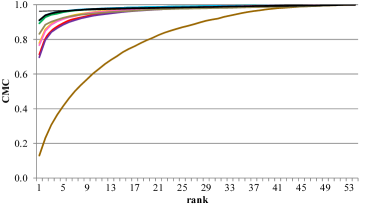
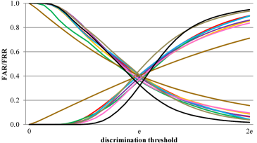
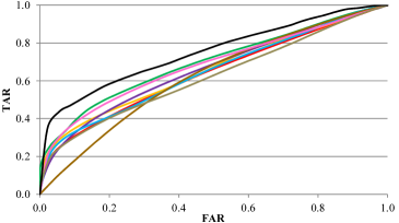
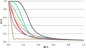
Figure 3: Four rank-based classifier performance metrics CMC (top left), EER-centered FAR/FRR (top right), ROC (bottom left) and RCL/PCN (bottom right).

	class separability coefficients				classification based metrics
method	DBI	DI	SC	FDR	CCR	EER	AUC	MAP
Ahmed [2]	189.31	1.1823	$-$0.1323	0.9213	0.7134	0.411	0.6387	0.1617
Andersson [3]	175.5	1.2047	$-$0.1117	0.9277	0.7787	0.413	0.6545	0.1926
Ball [4]	200.75	1.014	$-$0.14	0.982	0.6963	0.3906	0.6612	0.1454
Dikovski [5]	138.44	1.788	$-$0.0873	1.2803	0.8926	0.3625	0.6964	0.2582
Kwolek [6]	151.28	1.2027	$-$0.074	0.974	0.9089	0.4072	0.6477	0.2121
Preis [7]	2138.3	0.0313	$-$0.3756	1.0957	0.13	0.4041	0.6236	0.0579
Sinha [8]	166.83	1.3	$-$0.1256	1.0413	0.7666	0.3706	0.6809	0.1858
PCA+LDA	195.19	1.021	$-$0.084	0.8207	0.8314	0.447	0.6216	0.1643
MMC	96.2	1.8453	0.2227	1.278	0.9102	0.3223	0.7551	0.2996

Table II: Four class separability coefficients and supplementary rank-based classifier performance metrics related to Figure 3 for all tested gait recognition methods.

The goal of the MMC-based learning is to find a linear discriminant that maximizes the misclassification margin. This optimization technique appears to be more effective than designing geometric gait features. Figure 3 and in Table II indicate the best results: lowest DBI, highest DI, highest (and exclusively positive) SC, second highest FDR and, combined with rank-based classifier, the best CMC, FAR/FRR, ROC and RCL/PCN scores along with all CCR, EER, AUC and MAP. We interpret the high scores as a sign of robustness. Apart from performance merits, the MMC method is also efficient: relatively low-dimensional templates (see the third column in Table I) and Mahalanobis distance (6) ensure fast distance computations and thus contribute to high scalability.

IV Conclusions and Future Work

The field of pattern recognition has recently advanced to an era where best results are often obtained using a machine learning approach. Finding optimal features for MoCap-based gait recognition is not an exception. This work introduces the concept of learning robust and discriminative features directly from raw joint coordinates by a modification of the Fisher’s Linear Discriminant Analysis with Maximum Margin Criterion with the goal of maximal separation of identity classes. The introduced MMC method avoids instinctive drawing of ad-hoc features; on the contrary, they are computed from a much larger space beyond the limits of human interpretability. The collection of learned features achieves leading scores in four class separability coefficients and therefore has a strong potential in gait recognition applications. This is demonstrated by outperforming other methods in numerous rank-based classification metrics. We believe that MMC is a suitable criterion for optimizing gait features; however, our future work will continue with research on further potential optimality criterions and machine learning approaches.

Furthermore, we are investigating on whether these features can discriminate different people than exclusively who they are learned on. Can the number of learning identities be (much) smaller than the number of walkers encountered in the real operation? The main idea is to learn what aspects of walk people generally differ in and extract those as gait features. This is particularly important for a system to aid video surveillance applications where encountered walkers never supply labeled data and new identities can appear on the fly.

Acknowledgments

The data used in this project was created with funding from NSF EIA-0196217 and was obtained from http://mocap.cs.cmu.edu [15]. Our extracted database and implementation details of the compared methods are available at https://gait.fi.muni.cz to support reproducibility of results.

References

- [1] J. Valcik, J. Sedmidubsky, and P. Zezula, “Assessing Similarity Models for Human-Motion Retrieval Applications,” Computer Animation and Virtual Worlds, vol. 27, no. 5, pp. 484–500, 2016. [Online]. Available: http://dx.doi.org/10.1002/cav.1674
- [2] M. Ahmed, N. Al-Jawad, and A. Sabir, “Gait Recognition Based on Kinect Sensor,” Proc. SPIE, vol. 9139, pp. 91 390B–91 390B–10, 2014. [Online]. Available: http://dx.doi.org/10.1117/12.2052588B
- [3] V. O. Andersson and R. M. Araujo, “Person Identification Using Anthropometric and Gait Data from Kinect Sensor,” in Proc. of the Twenty-Ninth AAAI Conference on Artificial Intelligence (AAAI-15). AAAI Press, 2015, pp. 425–431. [Online]. Available: http://www.aaai.org/ocs/index.php/AAAI/AAAI15/paper/view/9680
- [4] A. Ball, D. Rye, F. Ramos, and M. Velonaki, “Unsupervised clustering of people from ’skeleton’ data,” in Proceedings of the Seventh Annual ACM/IEEE International Conference on Human-Robot Interaction, ser. HRI ’12. New York, NY, USA: ACM, 2012, pp. 225–226. [Online]. Available: http://doi.acm.org/10.1145/2157689.2157767
- [5] B. Dikovski, G. Madjarov, and D. Gjorgjevikj, “Evaluation of Different Feature Sets for Gait Recognition Using Skeletal Data from Kinect,” in 37th Intl. Convention on Information and Communication Technology, Electronics and Microelectronics, May 2014, pp. 1304–1308. [Online]. Available: http://ieeexplore.ieee.org/stamp/stamp.jsp?arnumber=6859769
- [6] B. Kwolek, T. Krzeszowski, A. Michalczuk, and H. Josinski, “3D Gait Recognition Using Spatio-Temporal Motion Descriptors,” in Proc. of Intelligent Information and Database Systems: 6th Asian Conference, ACIIDS 2014, Bangkok, Thailand, Part II, ser. LNCS, vol. 8398. Springer, Apr. 2014, pp. 595–604. [Online]. Available: https://doi.org/10.1007/978-3-319-05458-2_61
- [7] J. Preis, M. Kessel, M. Werner, and C. Linnhoff-Popien, “Gait Recognition with Kinect,” in 1st International Workshop on Kinect in Pervasive Computing, New Castle, UK, June 18–22, 2012, pp. 1–4. [Online]. Available: https://www.researchgate.net/publication/239862819_Gait_Recognition_with_Kinect
- [8] A. Sinha, K. Chakravarty, and B. Bhowmick, “Person Identification Using Skeleton Information from Kinect,” in ACHI 2013: Proc. of the Sixth Intl. Conf. on Advances in CHI, 2013, pp. 101–108. [Online]. Available: https://www.thinkmind.org/index.php?view=article&articleid=achi_2013_4_50_20187
- [9] V. N. Vapnik, The Nature of Statistical Learning Theory. New York, NY, USA: Springer-Verlag, 1995.
- [10] H. Li, T. Jiang, and K. Zhang, “Efficient and Robust Feature Extraction by Maximum Margin Criterion,” IEEE Transactions on Neural Networks, vol. 17, no. 1, pp. 157–165, Jan 2006. [Online]. Available: https://doi.org/10.1109/TNN.2005.860852
- [11] R. A. Fisher, “The Use of Multiple Measurements in Taxonomic Problems,” Annals of Eugenics, vol. 7, no. 2, pp. 179–188, 1936. [Online]. Available: https://doi.org/10.1111/j.1469-1809.1936.tb02137.x
- [12] P. N. Belhumeur, J. P. Hespanha, and D. J. Kriegman, “Eigenfaces vs. Fisherfaces: Recognition Using Class Specific Linear Projection,” IEEE Trans. Pattern Anal. Mach. Intell., vol. 19, no. 7, pp. 711–720, Jul. 1997. [Online]. Available: https://doi.org/10.1109/34.598228
- [13] M. Loog, R. P. Duin, and R. Haeb-Umbach, “Multiclass Linear Dimension Reduction by Weighted Pairwise Fisher Criteria,” IEEE Transactions on Pattern Analysis and Machine Intelligence, vol. 23, no. 7, pp. 762–766, Jul. 2001. [Online]. Available: https://doi.org/10.1109/34.935849
- [14] H. Su, Z.-W. Liao, and G.-Y. Chen, “A gait recognition method using L1-PCA and LDA,” in Proc. of the Eighth Intl. Conf. on Machine Learning and Cybernetics, vol. 6, Jul. 2009, pp. 3198–3203. [Online]. Available: https://dx.org/10.1109/ICMLC.2009.5212776
- [15] CMU Graphics Lab, “Carnegie-Mellon Motion Capture (MoCap) Database,” 2003, http://mocap.cs.cmu.edu.