Living document 3 1 4mm 90 current page.east

QUBIC Technical Design Report
The QUBIC collaboration

Preface

QUBIC, now in its construction phase, is dedicated to the exploration of the inflation age of the Universe. By detecting and characterizing the Cosmic Microwave Background B-mode polarization, QUBIC will contribute to find the “smoking gun” of inflation and to discriminate among the numerous models consistent with current data. The primordial B-modes (as opposed to E-modes) is the unique direct observational signature of the inflationary phase that is thought to have taken place in the early Universe, generating primeval perturbations, producing Standard Model elementary particles and giving its generic features to our Universe (flatness, homogeneity…).

Recent results from the BICEP2 and the Planck collaborations have brought the importance of the quest for B-modes to the attention of a wide audience well beyond the cosmology community. The original claim from BICEP2, contradicted by Planck later on has also shown how challenging the search for primordial B-mode polarization is, because of many difficulties: smallness of the expected signal, instrumental systematics that could possibly induce polarization leakage from the large E signal into B, brighter than anticipated polarized foregrounds (dust) reducing to zero the initial hope of finding sky regions clean enough to have a direct primordial B-modes observation.

QUBIC is designed to address all aspects of this challenge with a novel kind of instrument, a Bolometric Interferometer, combining the background-limited sensitivity of Transition-Edge-Sensors and the control of systematics allowed by the observation of interference fringe patterns, while operating at two frequencies to disentangle polarized foregrounds from primordial B mode polarization.

QUBIC is the only European ground based B-mode project with the scientific potential of discovering and measuring B-modes. It is the natural project for the European CMB community to continue at the edge-cutting level it has reached with Planck.

With the measurement of the Cosmic Microwave B-mode Polarization in two bands at 150 and 220 GHz, with two years of continuous observations from Alto Chorillos near San Antonio de los Cobres, Argentina, the first QUBIC module would be able to constrain the ratio of the primordial tensor to scalar perturbations power spectra amplitudes with a conservative projected uncertainty of $\sigma(r)=0.02$, while having a good control of foregrounds contamination thanks to its dual band nature.

Depending on the scientific and technological results of the first module we could envidage to construct more QUBIC modules operating at three frequencies (90, 150 and 220 GHz) that could feature design upgrades in order to achieve a higher sensitivity, and could preferentially be deployed in Antartica to take benefit of its exquisite atmospheric conditions. These could include different detectors (eg MKIDs), larger horn arrays or number of detectors, different optical combiner design, … QUBIC is therefore a project dedicated to grow and could be a Europen Stage-IV CMB Polarization experiment.

QUBIC has been and will be implemented through successive steps:

1. R$\&$D to design the instrument (now finalized)

2. Validation of the detections chain (now finalized)

3. Validation of the technological demonstrator (less detectors and horns than the final instrument, but in the nominal cryostat). This will occur in the course of 2017.

4. Construction and operations of the of the first module which will happen in the second half of 2017.

5. Optionaly, construction and operations of a number of additional modules to complete the QUBIC observatory.

More details can be found on the QUBIC website : http://qubic.in2p3.fr/QUBIC/Home.html

1 Science Case

1.1 Context: the Quest for primordial B-modes

1.1.1 Primordial Universe, Inflation and the CMB Polarization

Our understanding of the origin and evolution of the Universe has made remarkable progress during the last two decades, thanks in particular to the observations of the Cosmic Microwave Background (CMB). The diverse and more and more numerous probes, such as CMB anisotropies, SNIa, BAO (…) give complementary informations, enabling consistency tests of the standard cosmological model (aka $\Lambda\hbox{CDM}$ model). This concordance model is based on General Relativity and is parameterized, in its simplest form, with six parameters. From the determination of those cosmological parameters using the observations, we have learned that the Universe is spatially flat, contains a large fraction of dark matter, and experiences accelerated expansion. The latter can be accommodated within the Friedman-Lemaître framework through the presence of a mysterious dark energy $\Lambda$ (or cosmological constant).

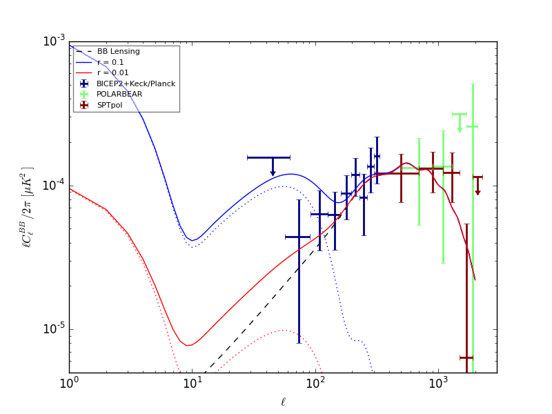
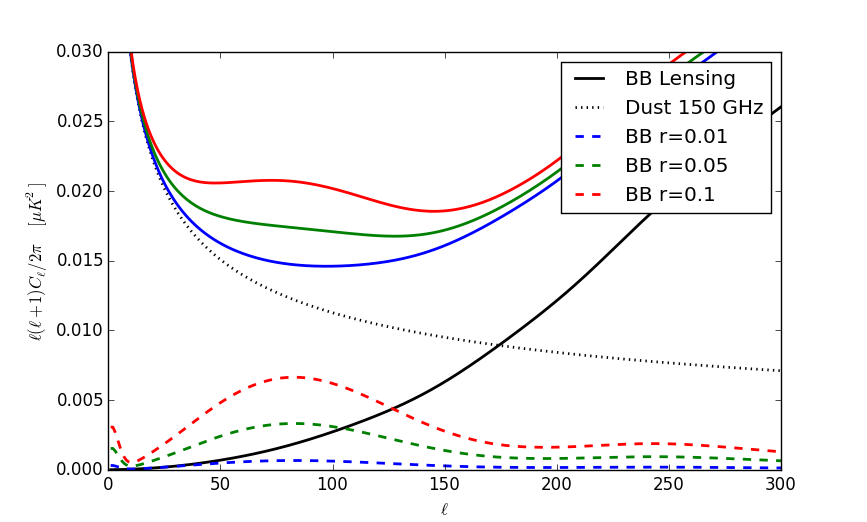
Figure 1: (left) Recent B-modes measurements compiled in  [sptpol], with results from BICEP2/Keck [bicep2] (dominated by dust), PolarBear [PolarBear], ACTpol [actpol] and SPTpol [sptpol] due to lensing. The reionisation and recombinations bumps can be seen at respectively $\ell\simeq 7$ and $\ell\simeq 100$. (right) Total B-modes (primordial + lensing + dust) expected signal for different values of the tensor-to-scalar ratio with dust level set by Planck and BICEP2 measurements [Ade:2015tva] (black dotted line).  

Regarding the most primordial Universe history (i.e. shortly – 10^-38 sec – after the Big Bang), all the observational data are up to now perfectly consistent with the inflation paradigm in which the young Universe undergoes a period of accelerated expansion that results in a flat, almost uniform space-time when inflation ends. Besides explaining flatness and homogeneity (which has originally motivated its introduction), inflation appears as the best theory able to produce the observed almost scale invariant spectrum for the Gaussian primordial density fluctuations without fine-tuning, only relying on the evolution of the quantum fluctuations of the scalar field(s) driving inflation. One of the most important predictions of inflation is that, on top of the density anisotropies (corresponding to scalar perturbations of the metric), it is expected to produce primordial gravitational waves (corresponding to tensor perturbations of the metric). This specific prediction of inflation remains to be tested and is the core motivation for the QUBIC instrument, together with the measurement of their amplitude to further constrain the inflation models.

CMB polarization can be decomposed into two modes of opposite parities: E-modes (with even parity) and B-modes (with odd parity). In total, four different power spectra describe the correlations of CMB temperature (T) and polarization (E and B) anisotropies. Density perturbations only give rise to E modes, while gravity waves are also source of B-modes. In other words, an observation of primordial B-modes would be the “smoking gun” betraying the presence of primordial gravity waves generated by inflation. B-mode detection is today one of the major challenges to be addressed in observational cosmology. This signal is parameterized using the tensor-to-scalar amplitude ratio $r$ which value would allow us to distinguish between various inflation scenarios and is directly related to the energy scale of inflation [baumann]. Theoretical predictions on the tensor to scalar amplitudes ratio are rather weak however but the simplest inflationary models predict r to be higher than 0.01 as the corresponding energy level would be too low with respect to Grand Unified Theories for smaller values or $r$. We plan to explore this very range (between 0.01 and 0.1) with QUBIC.

1.1.2 A major observational challenge

Unfortunately, B-modes appear to be very difficult to detect because of their small amplitude: a tensor-to-scalar ratio of 0.01 corresponds to polarization fluctuations of the CMB of a few nK while the well observed temperature fluctuations are around 100 microK. Even if such a sensitivity can be achieved using background limited detectors such as bolometers from low-atmospheric emission suborbital locations or from a satellite, the challenge to face for this detection remains huge because of two main reasons: instrumental systematics and foregrounds.

Instrumental systematic effects of usual telescopes (sidelobes, cross-polarization) may become too large to be disentangled from a small primordial B-mode signal. Indeed any instrument, even designed with care, exhibits cross-polarization, beam mismatch, inter calibration uncertainties, cross-talk, … All of these instrumental systematics mix the electric fields in the two orthogonal directions inducing a mixing between the Stokes parameters Q and U and possibly a leakage from intensity into polarization. This induces leakage from I and E into B-modes that, given the smallness of the primordial B-modes, may completely overcome those B-modes. A new generation of instruments achieving an unprecedented level of control of instrumental systematics is therefore needed for the B-mode quest. QUBIC was precisely designed with this objective.

B-modes anisotropies are also produced by foregrounds (summarized in the right panel of Figure 1):

1. The lensing of the B-modes by intervening large scale structure in the Universe converts part of the E-modes into B-modes, mostly at small scales($\ell\gtrsim 300$). The spectrum of those lensing B-modes however has a well defined shape and has been detected recently by PolarBear [PolarBear], ActPol [actpol] and SPTpol [sptpol] (see Figure 1, left panel). This contribution is not expected to affect the primordial B-modes detectability on the large scales observed by QUBIC (around the so-called recombination peak at l=100) if the tensor-to-scalar ratio is sufficiently high, but would become a strong limitation if r is below $\sim 0.01$.

2. Thermal emission from dust grains in the Galaxy is expected (and measured) to be linearly polarized due to the elongated shape of the grains which align along the magnetic field. The dust e.m. spectrum is different from the CMB one so that multiple frequencies (above 150 GHz) can be used to remove it and obtain cleaned maps of the CMB B-modes. This was the motivation for adding a 220 GHz channel in QUBIC besides the initial 150 GHz one.

3. Synchrotron emission from electrons swirling around magnetic fields in the Galaxy is also expected to produce B-modes. The synchrotron EM spectrum is falling with frequency so that it can be monitored with channels at lower frequencies that the CMB ones the same way as dust. Synchrotron polarization is not expected to be highly significant at 150 nor at 220 GHz, the QUBIC operation frequencies [Krachmalnicoff:2015xkg] [Fuskeland].

4. For ground based observations, atmosphere is also a possible source of contamination. However, the main effect of atmosphere is to increase the loading on the detectors in a time-variable manner that increases the variance of the data. A recent study with PolarBear data [JosquinAtmo] has shown that the polarization induced by atmosphere remains at a small level when observing from the Atacama plateau, which is known to be worse than in South Pole.

Searching for B-modes in the Cosmic Microwave Background polarization is therefore a major challenge that requires instruments observing at multiple frequencies with high sensitivity and unprecedented control of instrumental systematics. The current best upper-limit on r is r < 0.07 at 95% C.L.  [Ade:2015tva] and is obtained by combining BICEP2, Keck Array and Planck data.

1.1.3 Ongoing and planned projects

Two kinds of instruments have been used so far in the Cosmic Microwave Background polarization observations:

• Imagers where an optical system (reflective as in Planck or refractive as in BICEP2) allows us to form the image of the sky on a focal plane equipped with high sensitivity total power detectors. Bolometers have been successfully used because their intrinsic noise is lower than the photon noise of the observed radiation (so-called «background limited»). This is achieved by cooling the bolometers down to sub-Kelvin temperatures. The detection principle is that incoming radiation heats the bolometers whose temperature is being monitored through the variation of a resistance (resistively or using the normal-superconducting transition). Recently, Kinetic Inductance Detectors (KIDs) have been developped, they present the advantage of an easier fabrication process and natural ability for multiplexed readout (a major issue at cryogenic temperatures). Imagers directly measure the temperature on the sky in a given direction (with a resolution given by that of the telescope and horns) and therefore allow building maps of the CMB Stokes parameters I, Q, and U that further enables us to reconstruct T, E and B power spectra.

• Interferometers where the correlation between two receivers allows us to directly access the Fourier modes (known as visibilities) of the Stokes parameters I, Q and U without producing maps. The observation of interference fringes with an interferometer allows for an extra control of systematic effects in comparison with an imager. That explains why interferometers were used for the first measurements of sub-degree temperature anisotropies (with VSA [vsa]) and E-mode polarization (with CBI [cbi] and DASI [dasi]). However, they suffered from a degraded sensitivity due to their heterodyne nature: signals at the frequency of the CMB (from a few GHz to a few hundreds of GHz) need to be amplified and down-converted to lower frequencies before being detected. This amplification process adds an irreducible amount of noise that prevents such interferometers from being background limited. Furthermore, the complexity of traditional CMB interferometers (based on multiplicative interferometry, making the correlation by pairs of detectors) prevent them from growing to the large number of receivers that is now required to achieve the sensitivity needed for the B-mode quest (if N is the number of channels, their complexity increases as N² while that of an imager grows as N). This is the reason why, despite their better ability to handle instrumental systematics, interferometers have no longer been considered, until QUBIC, for CMB polarization observations.

Project	Country	Location	Status	Frequencies	$\ell$ range		$\sigma{(r)}$ goal
				(GHz)	value	Ref.	no fg.	with fg.
QUBIC	France	Argentina		150,220	30-200		0.006	0.01
Bicep3/Keck	U.S.A.	Antartica	Running	95, 150, 220${}^{1}$	50-250	[BicepMoriond]	$2.5\ 10^{-3}$	0.013
CLASS	U.S.A.	Atacama	$\geq 2016$	38, 93, 148, 217	2-100	[Class]	$1.4\ 10^{-3}$	0.003
SPT3G	U.S.A.	Antartica	2017	95, 148, 223	50-3000	[SPTMoriond]	$1.7\ 10^{-3}$	0.005
AdvACT	U.S.A.	Atacama	Starting	90, 150, 230	60-3000	[ACTMoriond]	$1.3\ 10^{-3}$	0.004
Simons Array	U.S.A.	Atacama	$\geq 2017$	90, 150, 220	30-3000	[SimonsArrayPres]	$1.6\ 10^{-3}$	0.005
LSPE	Italy	Artic	2017	43, 90, 140, 220, 245	3-150	[LSPE]	0.03${*}$
EBEX10K	U.S.A.	Antartica	$\geq 2017$	150, 220, 280, 350	20-2000	[EBex10K]	$2.7\ 10^{-3}$	0.007
SPIDER	U.S.A.	Antartica	Running	90, 150	20-500	[SpiderMoriond]	$3.1\ 10^{-3}$	0.012
PIPER	U.S.A.	Multiple	$\geq 2016$	200, 270, 350, 600	2-300	[Piper]	$3.8\ 10^{-3}$	0.008

Table 1: Summary of the main ground and balloon projects aiming at measuring B-modes. The label “fg” or “no fg” corresponds to the assumption on the foregrounds, numbers have been extracted from [Josquin]. [$*$] The LSPE value is an upper limit at 99.7$\%$CL. [1] Ref.  [Josquin] did not include this frequency. .

Most of the on-going or planned projects are lead by U.S. teams. They are all based on the concept of a traditional imager with a broad variety of technical choices regarding the modulation of the polarization, the optical setup, the detector technology, the frequency coverage or the instrument location. They also use different instrumental apertures, that sets the angular accuracy hence the multipole coverage and therefore are optimized for different science goals: high angular resolution instruments are better suited for the lensing B-modes study (allowing one to constrain neutrino masses for instance), and have published results on this (PolarBear, SPTpol, ACTpol) while low resolution suborbital instruments aim at detecting the recombination peak of the primordial B-modes at l=100. Satellite missions are considered by the community and aim at covering both science goals with the additional advantage of a full sky coverage allowing one to search for the reionization peak at l=7. However, no such mission has been selected up to now by Space agencies, neither in the U.S.A. nor in Europe. LiteBird is a possible mission to be flown in the early 2020 by the Japanese Space Agency (JAXA) and would be an extremely sensitive project (targeting r=0.001) with low angular resolution, therefore only focused on primordial B-modes.

Table 1 summarizes the situation in terms of competitors for QUBIC. We know since the BICEP2/Planck controversy that foregrounds cannot be neglected. This is why, when the foreground-free forecasted sensitivity of the QUBIC first module, from Argentina, is $\sigma(r)=0.01$, we can only achieve $\sigma(r)=0.02$ when accounting for realistic foregrounds. The observation efficiency is taken to be $30\%$ in those QUBIC sensitivity forecasts. Besides BICEP/Keck [Ade:2015tva] on the ground and the ballon-borne SPIDER experiment [fraisse_spider] which has already taken data in the same multipole range as QUBIC (namely targeting the recombination peak at $\ell\sim 100$), it is clear from this table that QUBIC is competitive and timely with respect to other competitors with the same target. High resolution experiments are more suited to the measurement of the lensing B-modes which should provide very exciting neutrino constraints. Although these projects claim they will measure primordial B-modes, this is not their primary goal and that they focus on the smaller angular scales because large angular scales are harder to reconstruct due to 1/f noise (from electronics and/or atmosphere). As a matter of fact, these experiments have never published data, even with temperature only, below a multipole of $\sim 300$. While having comparable sensitivity with the other experiments, QUBIC will offer this improved control of instrumental systematics that may be a decisive factor when reaching very low tensor-to-scalar ratio sensitivity.

1.2 Bolometric Interferometry and QUBIC

Most of the current projects aiming at detecting the B-mode radiation are based on the architecture of an imager because of its simplicity and the high sensitivity allowed by bolometers. However, imagers do not allow for the same level of control of instrumental systematics and could potentially reach a sensitivity floor because of E-modes leaking into B-modes.  Bolometric Interferometry is a novel concept combining the advantages of bolometric detectors in terms of sensitivity with those of interferometers in terms of control for systematics. It was initially proposed in 2001 by Peter Timbie (University of Wisconsin) and Lucio Piccirillo (University of Manchester). Two collaborations on both sides of the Atlantic (BRAIN in Europe and MBI in the U.S.A.) started to develop the concept and decided to merge their efforts in the QUBIC project in 2008. The QUBIC collaboration now includes six laboratories in France, all members of the CNRS (APC in Paris, LAL, IAS and CSNSM in Orsay and IRAP in Toulouse), three  Universities in Italy (Universitá di Roma – La Sapienza, Universitá Milano Bicocca and Statale in Milano), Manchester and Cardiff Universities in the UK and NUI/Maynooth in Ireland, three universities in the USA (University of Wisconsin at Madison, WI ; Brown University at Providence, RH ; Richmond University, VI). NIKHEF (Netherlands) have joined QUBIC in 2014.

1.2.1 The QUBIC design

QUBIC will observe interference fringes formed altogether by a large number of receiving horns with two arrays of bolometric detectors (operating at 150 and 220 GHz) at the focal planes of an optical combiner. The image on each focal plane is a synthesized image in the sense that only specific Fourier modes are selected by the array of receiving horns. A bolometric interferometer is therefore a synthetic imager whose beam is the synthesized beam formed by the array of receiving horns. The interferometric nature of this synthesized beam allows us to use a specific self-calibration technique that permits to determine the parameters of the systematic effects channel by channel with an unprecedented accuracy [Charlassier] [Bigot]. As a comparison, an imager can only measure the effective beam of each channel. We therefore have an extra-level of systematics control. The use of bolometric detectors allows us to reach a sensitivity comparable to that of an imager with the same number of receivers [Hamilton].

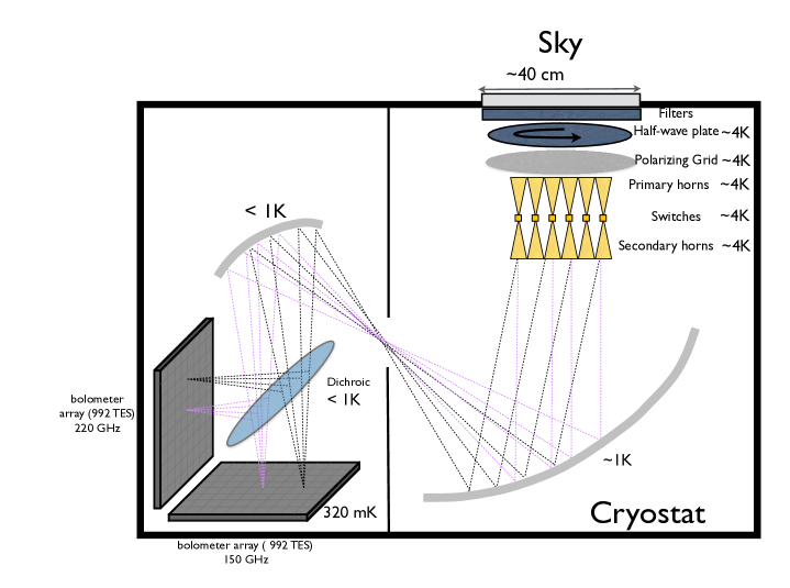
Figure 2: Sketch of QUBIC (see text for explanation)

The QUBIC instrument is made (see Figure 2) of a cryostat cooled down to 4K using pulse-tubes. The cryostat is open to the sky with a 45 cm diameter window made of high-density polyethylene (HDPE) providing an excellent transmission and mechanical stiffness. Right after the window, filters ensure a low thermal load inside the cryostat and a rotating Half-Wave-Plate (HWP) similar to that of the Pilot instrument [salatino] modulates the polarization. Then, a polarizing grid selects one of the two polarization angles w.r.t the instrument. An array of 400 corrugated horns (called « primary horns » designed to be efficient throughout the 150 and 220 GHz bands with a $\approx 13$ degrees FWHM at 150 GHz) selects the baselines observed by QUBIC. These primary horns are immediately followed by back-horns re-emitting the signal inside the cryostat towards an « optical combiner » which is simply a telescope that combines on the focal plane the images of each of the secondary horns in order to form interference fringes. Before the focal plane, a dichroic plate splits the signal into its 150 and 220 GHz components that are each imaged on a focal plane equipped with 1024 Transition-Edge-Sensors (TES) from which 992 are exposed to the sky radiation (blind ones are used for systematics studies) cooled down to 320 mK and read using a multiplexed cryogenic readout system based on SQUIDs and SiGe ASIC operating at 4K. Finally, the signal measured by each detector p at in the focal plane with frequency $\nu$ at time t is:

$$R(p,\nu,t)\ =\ S_{I}(p,\nu)+\cos\left[4\varphi_{\mathrm{HPW}}(t)\right]S_{Q}(p,\nu)+\sin\left[4\varphi_{\mathrm{HPW}}(t)\right]S_{U}(p,\nu)$$ (1)

where $\varphi_{\mathrm{HWP}}(t)$ is the angle of the HWP at time t, $S_{I/Q/U}$ the sky signal at frequency $\nu$ convolved with the synthesized beam (see Figure 3). With a scanning strategy offering a wide range of polarization angles on the sky and thanks to the HWP rotation, one can recover the synthesized images of each of the three Stokes parameters I, Q and U. In contrast with traditional interferometry, the observables of QUBIC are not the visibilities (Fourier Transform of the observed sky for modes corresponding to the baselines), but the synthesized image, which is nothing else but the observed sky filtered to the modes corresponding to the baselines allowed by our instrument. This particular feature is a crucial one in QUBIC as each of these modes can be calibrated separately using the « self calibration » procedure (see section 1.2.3 and [Bigot]) allowing QUBIC to reach an unprecedented level of instrumental systematics control.

One important aspect of the QUBIC design is the presence of the polarizing grid right after the half-wave plate, ie very close to the sky. It may appear undesirable from the sensitivity point of view to reject half of the photons at the entrance of the instrument. However, this a very nice feature from the point of view of polarization systematics because this is associated with bolometers that are not polarization sensitive: the rejection of the undesidered polarization with the polarizing grid is very efficient and whatever the cross-polarization of the rest of the instrument, the detectors will measure the polarized sky signal modulated by the HWP. This means that we expect a very low level of instrumental cross-polarization for QUBIC.

1.2.2 The QUBIC synthesized beam and map-making

In QUBIC, each primary horns pair defines a baseline (a Fourier mode on the sky) that is transmitted through the instrument and forms an interference fringe on the focal planes. In the standard « sky observing » mode, the fringes formed by all the baselines are coherently combined on the focal and form a synthesized image of the sky, which is the sky image convolved by the QUBIC synthesized beam than can be calculated from the combination of all baselines.

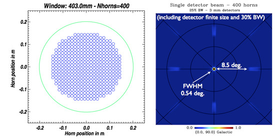
Figure 3: QUBIC primary horn array and corresponding beam on the sky for the central detector of any of the two focal planes.

The QUBIC horn array and synthesized beams are shown in Figure 3. As can be seen on this Figure (left panel), the horn array, although enclosed in a circle to optimize the window occupation, respects a regular square grid pattern that has been shown to ensure a coherent summation of redundant baselines which is the key aspect offering to a bolometric interferometer a comparable sensitivity to an imager [Hamilton] [Charlassier].

The synthesized beams shape is significantly different from the beam offered by a classical imager and typical of that of an interferometer: it has a central peak, with 0.54° FWHM and has replications around, damped by the primary 14° FWHM that are due to the fact that the primary horn array has finite extension. These replications are not sidelobes as they are a desired feature of an interferometer that only observes well defined and well « calibrable » baselines (see Sect. LABEL:selfcalsect). It however makes the map-making procedure much more complicated than with an imager as it involves partial deconvolution to disentangle the small contamination by secondary peaks with respect to the main one.

We have shown that using super-calculators and a specific map-making algorithm based on « inverse problem solving » [chanial], one can recover the input I, Q and U maps provided the fact that the scanning strategy offers a wide enough variety of polarization angles on the sky (which is ensured by the combination of sweeps in azimuth with constant elevation and the rotation of the Half-Wave-Plate, cf. Figure 4 and Figure 5).

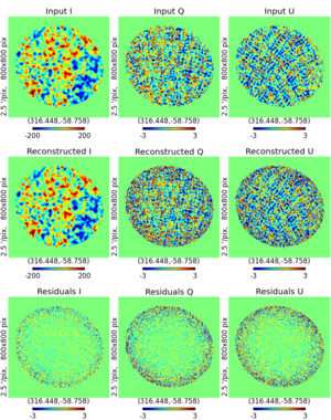
Figure 4: (left) Current results with the QUBIC mapmaking under the Gaussian peaks assumption. First row shows the input I,Q and U maps in the region observed by QUBIC, second row shows the recovered maps using the full simulation pipeline, last row shows the residuals w.r.t. the input maps.

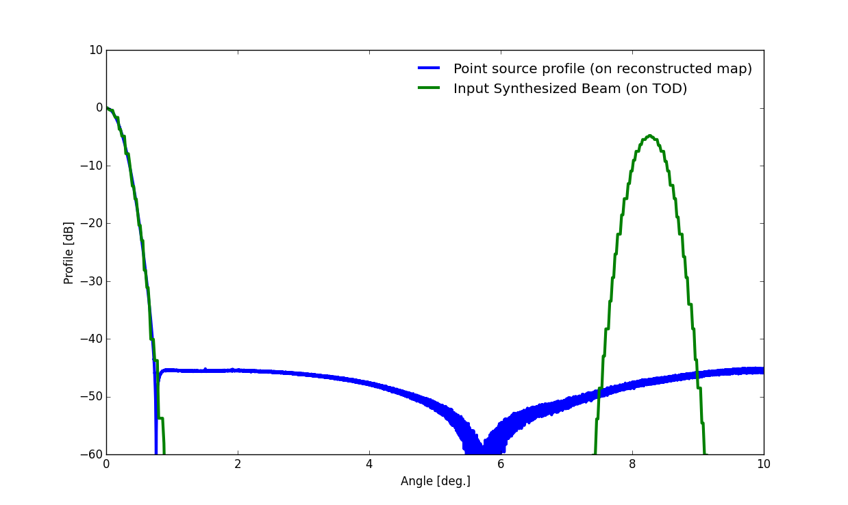
Figure 5: Results of the current version of the map-making: the multiple –peaked feature of the synthesized beam (green) present in the TOD is deconvolved efficiently in the maps where we show the recovered profile for a point source (blue line). The achieved resolution (FWHM of the blue central peak) is 23.5 arcmin.

1.2.3 Self-calibration and the systematic effects mitigation with QUBIC

Interferometry is known [Timbie] to offer an improved control of instrumental systematics with respect to direct imaging thanks to the observation of individual interference fringes that can be calibrated individually. This feature is conserved with bolometric interferometry, in QUBIC, thanks to the presence of electromagnetic switches between the primary and secondary horns (cf. sections  2.3.4 and  LABEL:switch). This apparatus consists in a waveguide that is closed or open using a cold (4K) shutter operated by solenoid magnets. In the self-calibration mode, pairs of horns are successively shut when observing an artificial partially polarized source (we do not need to know its polarization). As a result, we can reconstruct the signal measured by each individual pairs of horns in the array and compare them. As redundant baselines correspond to the same mode of the observed field, a different signal between them can only be due to photon noise or instrumental systematics. Using a detailed model of the instrument incorporating all possible systematics (through the use of Jones matrices for each optical component), we have shown that we can fully recover all of these parameters through a non-linear inversion involving hundreds of parameters (horn locations and beams, components cross-polarization, detector inter calibration, …). The updated model of the instrument can then be used to reconstruct the synthesized beam and improve the map-making, reducing the leakage between Stokes parameters. We have shown in [Bigot] that with 2.5% of the observing time, we can reduce the impact of the instrument systematics on the E to B leakage to a level allowing us to measure the B modes down to r=0.05 (see Figure 6). No such feature exists with a usual imager justifying the fact that QUBIC will have extra-control on instrumental systematics with respect to all the other running or planned instruments listed in Table  1.

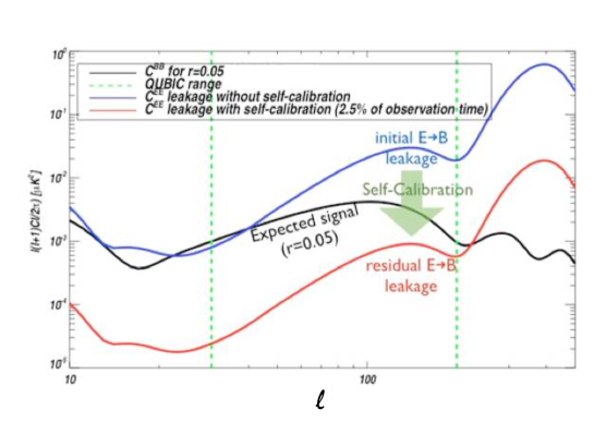
Figure 6: “Self-calibration” simulated result [Bigot]. The leakage from E to B due to instrumental systematics is reduced by more than an order of magnitude spending only 2.5% of the observation time on self-calibration.

1.3 QUBIC sensitivity to B modes

The first module of QUBIC will be installed in Argentina, on the Puna plateau in the Salta Province, near the city of San Antonio de Los Cobres, on the site of the LLAMA experiment (cf. Sect. LABEL:argentina for more details). Still, in the initial phase of the project, we considered installing QUBIC in Dome C, Antartica. For this reason, some results presented below refer to this site.

1.3.1 E/B power spectra from realistic simulations

The outputs of the mapmaking are I, Q and U Stokes parameters maps. However, the polarized fields of interest for cosmology are the scalar E and B fields instead of the spin-2 Q and U. They are related through a non-local transformation in harmonic space that is trivial when full sky Q and U maps are available. However, on a cut sky (a few percent of the celestial sphere for QUBIC), this transformation cannot be applied anymore since the Spherical Harmonics are no longer a complete basis. As a result, some of the modes are ambiguous (neither E nor B) and even in the absence of instrumental systematics, the cut sky induces massive leakage of E into B when just expanding the cut sky Q and U maps onto E and B power spectra. This mixing is however easy to revert as we know the exact geometry of the cut-sky. Unfortunately, although this inversion is unbiased and allows to recover unaltered E and B fields in average, the variance of the recovered fields contains contribution from both the sample variance of E and B so that the uncertainty on the small B field is largely dominated by the E sample variance [Tristram]. It is nonetheless possible to reduce the non-optimality of the B measurement by applying apodization functions [smith] [smith-zalda] [grain]. Finally, near-optimality can be reached (within a factor $\sim 2$) but requires a large amount of work with simulations in order to find the optimal apodization scheme for the Q and U maps.

Figure 7 shows in red the anticipated error bars on the 150 GHz channel assuming a perfect cleaning of the dust by the 220 GHz. They have been calculated using a full end-to-end Monte-Carlo Simulation (from time-ordered data to maps) for Dome C.

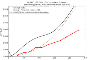
Figure 7: Full end-to-end Monte-Carlo simulation (from time-ordered data to maps and then to power spectra) error-bars (dispersion), at 150 GHz, assuming a perfect dust cleaning from the 220 GHz channel, are shown in red along with the expected signal from B-modes for r=0.05 for observations from Dome C.

1.3.2 QUBIC Sensitivity to B-Modes

Thanks to the extreme dryness of the Dome C site in Antarctica, the atmospheric emission in the millimeter wavelengths is extremely small [Tomasi] [Battistelli]. The Precipitable Water Vapor average in Dome C has been measured to be 0.6mm in January and well below 0.5mm the rest of the time. By comparison, it is below 0.5mm only 50% of the time in Chajnantor, Chile, where a number of B-modes experiments are installed (see Table 1). The QUBIC detectors, cooled down to 320mK, will be background limited, where the background is dominated by the atmosphere. We will therefore fully benefit from the former extreme location which would ensure QUBIC to have an exquisite sensitivity. Another advantage of being close to the South Pole is that the interesting fields in the sky (with minimal dust contamination [Adam:2014bub]) are not far from the Southern Equatorial Pole and therefore visible 100% of the time above 30 degrees elevation from Concordia, while this is not the case from Argentina, nor Chile where several other CMB observatories are based, forcing these experiments to define multiple observation fields which is not optimal. Expected errors on the B mode spectra obtained from Dome C are shown on the left panel of Figure 8.

We have performed full likelihood forecasts for QUBIC including lensing B-modes and dust foregrounds at the level measured by Planck in the BICEP2 field [Planck Intermediate Results XXX, 2014]. We use our two bands to form three cross power-spectra (150x150, 150x220 an 220x220) and multipole range from 25 to 300 to constrain the dust spectral index and primordial tensor-to-scalar ratio (dust amplitude is fixed by Planck 353 GHz). Those results (see Figure 8 right) show that using the two bands of QUBIC alone (blue) or with Planck 353 GHz added (red) allows to reach $\sigma(r)=0.01$ while this value goes down to $\sigma(r)=0.006$ in the absence of foregrounds (green). These forecasts assume two years of continuous observations from Dome C, Antarctica and an overall 30% efficiency. It is worth noting that Planck 353 GHz does not bring much gain with respect to QUBIC dual band (difference between red and blue).

Finally, when accounting for all the aspects, QUBIC, when deployed in Argentina, will reach $\sigma(r)=0.01$ in two years of observation with an overall 30% efficiency as quoted in Table 1. (see also Figure LABEL:fig107, more details on the site comparison can be found in Section {siteComparison).

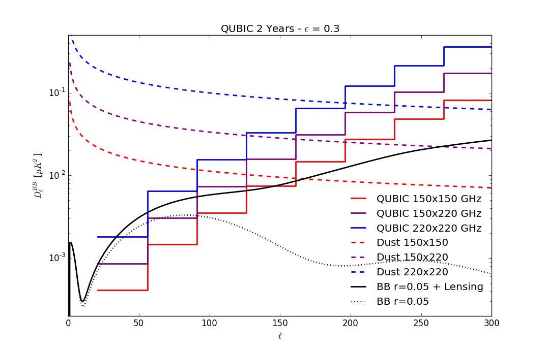
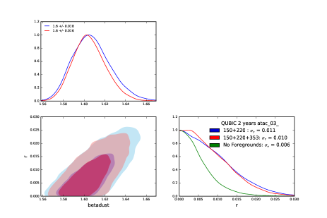
Figure 8: (left) Expected noise-only error bars for QUBIC for the three BB cross-spectra that can be formed along with r=0.2 and dust levels extrapolated following [Adam:2014bub] for the BICEP2 field. (right) Expected forecasts on dust spectral index and tensor-to-scalar ratio with QUBIC using a full likelihood with three configurations: QUBIC alone (blue), QUBIC with Planck 353 GHz information added (red), QUBIC if no foregrounds were present (green). The sensitivities on r are estimated from a marginalization over the dust spectral index and assume 2 years of continuous observations from Dome C and an overall efficiency of 0.3.

2 Overall Description of QUBIC

2.1 Main characteristics of the Instrument

The final sensitivity and deep control of systematics quoted in the previous section assumes that a series of requirements are fulfilled. They are listed in this section. The technical details on how these requirements are fulfilled in the instrument design are detailed in the rest of the Technical Design Review. Basic characteristics of the instrument are summarized in table 2. The QUBIC detectors (TESs) are cooled down to 320 mK thanks to a ${}^{3}$He/ ${}^{4}$He adsorption refrigerator. They are illuminated by an optical system (optical combiner, horns,…) cooled down to 1K. This experimental system is encased in a liquid-free cryostat housing a Pulse Tube cryocooler with base temperatures of 40K and 4K respectively for the 1st and 2nd cryogenic stage. Summaries of the characteristics of these various parts are listed below, and detailed further in this document.

Frequency channels	150 and 220 GHz
Bandwidth	25%
Number of horns (interferometric elements)	400
Primary beam FWHM at 150 GHz	12.9 degrees
Primary beam FWHM at 220 GHz	15 degrees (not gaussian)
Number of detectors	2x1024

Table 2: General requirements on the bolometric interferometer design.

The QUBIC instrument is composed of the following elements (see Figure 2) :

Optical Chain :
The optical chain of the QUBIC instrument starts from the window, opportunely coated with antireflection coating, directly observing the sky and extends to the detectors. It also includes the external baffling of the instrument that prevents ground pickup on the detectors.

QUBIC horns are quasi diffraction-limited apertures at 150GHz. This implies a relationship between their operating frequency, beam FWHM and aperture size: S$\Omega\sim\lambda^{2}$ which conditions their size to be 13.3mm (an internal diameter of 12.3mm to which 1 mm of metal wall thickness is added) for single mode operation at 150 GHz (HE11). The same horn structure support three modes at 220 GHz (HE11, TM02, EH21), with a consequently larger FOV (15 degrees, as shown in Table 2) and increased throughput. This gives its dimensions to the whole instrument.

The size of the horn array is thus 33.078 cm diameter as shown on Figure 3 (left hand side), driving the requirements summarized in table 3. The horns need to have a low level of cross polarization (< -25dB) and secondary lobes (< -20dB), and to transmit a large fraction of the incoming power (Return Loss < -25dB) across both 150 and 220 GHz bands.

Horn diameter (internal)	12.33 +/- 0.1 mm
Back-to-Back Horn array diameter	33.078 cm
Horn Return loss across the bands	< -25 dB
Horn secondary lobe level	< -20 dB
Horn cross-polarization level	< -25 dB
Horn interaxis	< 14 mm

Table 3: Requirements on horns

Window diameter	39.9 cm
Filters diameters	39.2 cm
Polarizer diameter	32.6 cm
Half-Wave plate diameter	32.7 cm
Half-Wave plate, filters and polarizer transmission	-0.2 dB
Half-Wave plate, filters and polarizer cross-polarization	-20 dB

Table 4: Requirements on cold optics chain

On the other hand, the detector size needs to be approximately the observed wavelength (2mm at 150 GHz) so that the overall $\sim$ 1k detectors array has a diameter of about 11 cm if it is maximally filled (which is of course highly desirable). This implies a focal length for the optical combiner of $f\sim$ 330mm [OSulli2015]. Such a focal length was found to be achievable with a minimal level of optical aberrations with an off-axis Gregorian system with the following characteristics: (1) it is nearly telecentric, (2) it fulfills the Rusch and Mizuguchi-Dragone condition, (3) it features a field of view largely diffraction limited with with Strehl ratio >0.8 within +/- 4.9 degrees [Gayer]. The requirement for the amount of optical aberrations was that the sensitivity loss is less than 10% when calculated by the ratio of the synthesized beam with and without optical aberrations. Requirements on cold optics and mirrors are summarized on Tables 4 and 5.

The different diameters have been calculated assuming that 95$\%$ of the power goes through the aperture, but similar values have been calculated to get 99$\%$ of the power.

Optical combiner focal length	30 cm
Number of mirrors	2
M1 shape and diameter	480mm x 600mm -
M2 shape and diameter	600mm x 500mm -
Optical combiner sensitivity loss from aberrations	< 10%

Table 5: Requirements on mirrors and optical properties

The possibility to monitor departure from idealities is provided by the self-calibration procedure. This procedure (see Sect. LABEL:selfcalsect) is indeed one of the main advantages of QUBIC with respect to other more traditional designs (see Sect. 1.1.3). In order to perform it efficiently, one needs to be able to switch on and off some of the horns while observing a calibration source. This requires waveguide switches placed in between the back-to-back horns. Such switches need to be closed enough when in off position (-80 dB) while open enough when set to the on position (-0.1 dB). Both of these criteria need to be fulfilled simultaneously across the 150 and 220 GHz bands. The switches also need to have low cross talk between neighbouring switches. The switching between on and off needs to dissipate minimal power at the 4K stage (60 mW) in order not to heat this stage and perturb observations. Such requirements are summarized on Table 6

Switches OFF transmission	-80 dB
Switches ON transmission	-0.1 dB
Switches Cross-talk	-40 dB

Table 6: Requirements on switches

External shields are required to prevent ground pickup in the detectors and make sure that photons coming from a large angle with respect to the optical axis are absorbed or reflected before entering the cryostat. This is achieved thanks to:

• a cylindrical forebaffle attached to the cryostat with a 1m length and a $14\deg$ opening angle. This allows to reduce by more than 20dB the radiation coming from 20deg < $\theta$ < 40deg from the optical axis, and by more than 40dB beyond.

• an external shield around the instrument mount or the experiment module’s roof (therefore fixed with respect to the ground) that allows a reduction of the radiation by another 40dB beyond 80 degrees from the zenith and minimize scan synchronous pick-up.

Baffling reduction 20deg < $\theta$ < 40deg	-20 dB
Baffling reduction 40deg < $\theta$ < 80deg	-40 dB
Baffling reduction $\theta$ > 80deg	-80 dB

Table 7: Requirements on the external shields

Detectors :
Transition Edge Sensors (TES) are the state of the art of bolometric detectors already employed in several millimetric and sub-millimetric astronomical experiments all over the world. They have been chosen as detectors for the QUBIC first module, relying on the extensive developments made in France over the last few years. We may however consider other types of detectors such as KIDs (Kinetic Inductance Detectors) for future QUBIC modules as they may offer an easier fabrication and readout, and larger scalability although they are not yet completely competitive in terms of noise with the TES.

A QUBIC TES focal plane is made of an array of 4$\times$256-pixels arrays disposed in an overall diameter of the order of 110 mm. The TES matrix for one focal plane of "QUBIC 1st module" is made of four identical pieces. The full focal plane TES matrix will have a quasi-circular shape as shown in Figure 9.

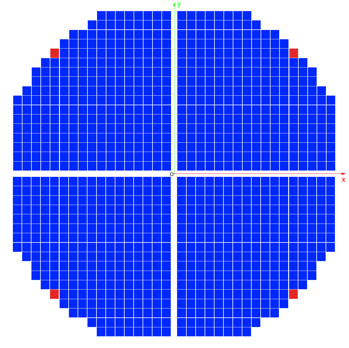
Figure 9: schematic "top-view" of the TES bolometers for one focal plane of the QUBIC 1st module. Active detectors are shown in blue.

A quarter of a focal plane is composed by 248 "usable" TES elements plus 8 blind sensors for $1/f$ noise monitoring. Thus a full focal plane include 992 "usable" TES bolometers, and the QUBIC 1st module will have 1984 usable TES. A quarter of a focal plane is presented in Figure 10.

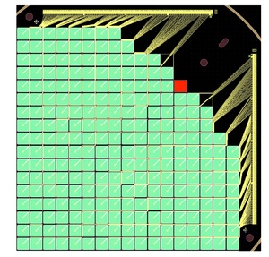
Figure 10: Picture of a TES array covering a quarter of the focal plane. Yellow lines are wires used for the reading of the TESes signal. The TES in red is not used.

The shape of one single TES and its electromagnetic wave absorber part are shown on Figure 11.

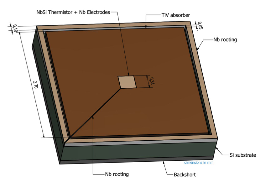
Figure 11: (left) Picture on one of the QUBIC focal plane TESes ; (right) Absorbing part of one TES (in blue).

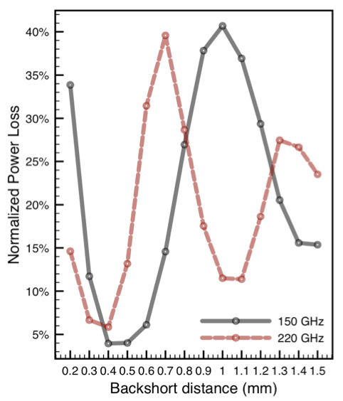
Figure 12: Simulated power loss of a detector at 150GHz and 220GHz with respect to backshort distance. An optimal value for the backshort is 400$\mu$m.

As mentioned above, the detector size is approximately defined by the central wavelength of the 150 GHz band, namely 2.7mm. Detectors, however, need to exhibit the same efficiency at 220 GHz as at 150 GHz. This efficiency is driven by the thickness of the backshort below the detector plane. We have set the power loss requirement at 10% for each and as it will be seen in Figure  12, we achieve 4% at 150GHz and 6% at 220 GHz. The number of detectors is determined by the required fraction of the secondary beam from the horns to be integrated in the focal plane. The requirement of 80% of the power integrated sets the number of detectors to 992, namely 4 wafers of 256 TES assembled together (minus the 8 blind detectors per wafer). We require that the fabrication yield of the TES is larger than 90%.

TES size	2.6 mm
Power loss on TES	< 10%
Power integrated on focal plane	> 80%
Number of bolometers / focal plane	1024
Number of 256 TES wafers	4
Fraction of operational detectors / wafer	> 90%

Table 8: Requirements on the TES detectors

In order to ensure a fruitfull exploitation of the QUBIC instrument data, the detectors sensitivities need to be close to the background limit, despite the fact that the focal planes are cooled down to 320 mK. Such a situation is achieved with TES noise below $5.10^{-17}W/\sqrt{Hz}$. We also require the time constants to be less than 10ms. Accordingly, the data rate for scientific data is required to be 100 Hz.

Detector stage temperature spec.	350 mK
Detector stage temperature goal	320 mK
Bolometers NEP	$5.10^{-17}\hbox{W.Hz}^{-1/2}$
Bolometers time constant	< 10 ms
Number of bolometers / focal plane	1024
Number of 256 TES wafers	4
Scientific Data sampling rate	100 Hz

Table 9: Requirements on the sensitivity

Cryogenics :
The whole instrument will be integrated in a cryostat that needs to be operated without the use of cryogenic liquids in order to be usable in any remote observation site. The 4K stage is therefore ensured thanks to a Pulse Tube Cooler achieving at least 1 W of cooling power at 4K. The electrical consumption of the Pulse Tube Cooler was required to be less than 15kW. A further requirement on the Pulse Tube Cooler is that it remains with unchanged cooling efficiency when the instrument is tilted in elevation during observations in the range required by the scanning strategy (30 to 70 degrees elevation, so $\pm$ 20 degrees). The 1K stage (secondary and primary mirrors, dichroic and detector structure) will be achieved using a ${}^{4}$He sorption fridge. The cryogenic stage for detectors will be ensured through a ${}^{3}$He/${}^{4}$He sorption cooler achieving a cooling power of at least 20$\mu$W at this temperature.

In order to be easily transported, the outer dimensions of the diameter of the cryostat is required not to exceed 1.6m and the height 1.8m. This requirement sets the dimensions of the whole internal cryogenic architecture. The weight of the instrument should not exceed 800 kg in order to be still transportable by helicopters if needed.

4K cooling	Pulse Tube Cooler
Pulse Tube Cooler 4K cooling power	>1 W
Pulse Tube Cooler Electrical consumption	< 15 kW
Pulse Tube Cooler angle range	+/- 20 degrees
1K stage refrigerator	${}^{4}$He sorption fridge
1K cooling power	>2 mW
detector stage refrigerator	${}^{3}$He/${}^{4}$He Sorption Cooler
detector stage cooling power	> 20$\mu$W
Instrument Diameter	< 1.6m
Instrument Height	< 1.8m
Instrument Weight	< 800 kg

Table 10: Requirement on cryostat and cryogenics

The overall internal structure of the cryostat will hold the horns+switches assembly, the mirrors, the dichroic and the detectors. It is cooled down to 1K. Such an assemble needs to weight less than 150 kg in order to prevent a too long cooling time for the cryostat. It also needs to bend by less than 400$\mu$m when the elevation of the instrument varies in the observation range (30 to 70 degrees). The heat conduction of the attaches of this structure need to be less than 2$\mu$W.

Internal Structure weight	< 150 kg
Internal Structure temperature spec.	<1.4K
Internal Structure temperature goal	1 K
Internal Structure bending for +/- 20 deg.	< 400$\mu$m
Internal Structure attaches heat conduction	< 2$\mu$W
Internal Structure rotation	< 0.2°

Table 11: Requirements on instrument internal structure

Self-calibration source :
This external calibrator is an active source able to radiate a typical power of few mW through a feedhorn with a well-known beam, and a low level of cross-polarisation (typically < -30 dB). Two similar systems, including a microwave sweeper followed by a cascade of multipliers, will be used to generate quasi- monochromatic signals to span both QUBIC bands. The external calibrator will be in the far-field of the interferometer, which means at about 40m. For this reason, it will be installed on top of a tower nearby the instrument. Due to the extreme environment conditions, the sources will be installed in an insulation box, suitable to maintain the devices in the desired temperature range.

We resume the basic specification of the sources in Table 12. More details are given in Section LABEL:calibSource2.

Frequency coverage	110-170 GHz & 170-260 GHz
power output spec.	5 mW
power output goal	1 mW
Operation modes	CW + amplitude modulation
Polarisation	Linear
Cross-polarisation	${\leq}$ -30 dB
Weight (estim., including insulation box)	10 kg

Table 12: Requirements on calibration sources

The tower must be around 40 m tall, and endowed with a lift to carry the source box and other equipment on top. A platform must be accessible at least for one person to operate the source and/or perform basic maintenance and/or to switch from 150 GHz to 220 GHz channel if required (we might consider the option of a source having a single microwave sweeper, but two different multiplier chains).

In order to avoid uncontrollable power fluctuations during self-calibration, we require stability against the wind: the lateral displacement of the platform on top shouldn’t exceed ± 20 cm with respect to the nominal position.

Mount :
The main requirements on the mount system are summarized in table 13.

Maximal diameter	2500 mm
Maximal height	2500 mm
Mass (without the instrument)	< 2300 kg
Mass to be supported by the mount	700 kg
Diameter of the instrument	1600 mm
Height of the instrument with forebaffle	1800 mm
Electrical consumption of the mount	< 1 kW
Rotation in azimuth	-220${}^{\circ}$ / +220${}^{\circ}$
Rotation in elevation	+30${}^{\circ}$ / +70${}^{\circ}$
Rotation around the optical axis	-30${}^{\circ}$/ +30${}^{\circ}$
Pointing accuracy (all axis)	< 20 arcsec
Angular speed (all axis)	Adjustable between 0 and 5${}^{\circ}$/s with steps < 0.2${}^{\circ}$/s

Table 13: General requirements on the mount system.

Slow control / data storage :

Four operating modes have been identified:

• Passive mode (no signal is acquired),

• Diagnostic mode (acquisition of diagnostic data such as temperatures),

• Calibration mode (used during observation of calibration sources, acquisition of bolometric, matrix thermometer, mount, switches, diagnostic and calibration sources data),

• Observation mode (acquisition of science data during sky observation, i.e. bolometric, matrix thermometer, mount and diagnostic data).

In the nominal observation mode (with an acquisition frequency of the scientific signal tuned at 2 kHz), the data rate (including raw and scientific signals, excluding house keeping signals) of the instrument will be 0.6 Mo/s. At that acquisition frequency, the needed data storage will be 20 To/year (see also section LABEL:datastore and tables LABEL:table16 and LABEL:table17).

The slow control of the instrument allows to operate properly the overall system and especially the cryogenic system. It will be implemented in the QUBIC studio data acquisition system which has all the needed interfaces already implemented (serie, USB, GPIB…). All subsystems will provide their slow control system which will be further interfaced with QUBIC studio.

2.2 Cryogenic systems

2.2.1 Cryostat design / Mechanic architecture and CAD

The cryogenic system of QUBIC aims at cooling the detector arrays at 0.3K, the beam combiner optics at 1K, and the rotating HWP, the polarizing analyzer, the horn array, and the switches at 4K. It is based on:

• A self-contained 3He refrigerator cooling the detector arrays

• A self-contained 4He refrigerator pre-cooling the 3He fridge and cooling a large 1K shield surrounding the optical system (the beam combiner optic)

• Two 1W pulse-tube (PT) refrigerators working in parallel and cooling the experiment volume at 3K and the surrounding radiation shield at 40K respectively

• A large vacuum jacket surrounding the entire system, including a large (50 cm) optical window

• Heat switches, Heaters, Thermometers, Control Electronics to run the system.

In the following we describe the basic design choices, and the dimensions and interfaces of the cryogenic system.

2.2.2 Cryostat vacuum

The purpose of the outer shell of the cryostat is to allow the setup ot operate under high-vacuum conditions in the internal volume of the cryostat, to support all the internal elements, and to permit mm-wave radiation under study to reach the cryogenic part of the instrument through the optical window. The size of the outer shell of the cryostat is driven by the volume of the cryogenic instrument, which includes the polarization modulator, the horns array, the beam combiner mirrors, and the focal plane assembly, for a total volume of the order of $1\ m^{3}$. The cryostat has been designed around the cryogenic instrument, and its dimensions are a trade-off between the total size limit imposed by the transportation and the need for sufficient thermal insulation between the cryogenic instrument and the room-temperature shell.

The resulting vacuum shell has a diameter of 1.4m and a height of 1.55m. Its shape and structure has been optimized for withstanding the stress from atmospheric pressure outside and vacuum inside, with sufficient safety factors. The structure is made out of Aluminium alloy sheets, roll-bent and welded, reinforced by a stiffening ribs structure. The vacuum jacket is obtained by closing a vertical cylinder with two flanges (using indium seals) as shown in Figure 13. The axes of the two PTs are tilted by $40\deg$ with respect to the vertical, to allow optimal elevation coverage during the observations of the sky at the latitude of operation, while maintaining the Pulse Tube head close to the vertical position where its operational performance are maximized.

Figure 13 also shows the two pulse-tube (PT) heads, mounted on dedicated flanges on the cylinder. The top flange differs from the bottom one because it includes the vacuum window.

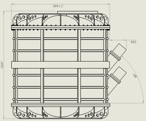
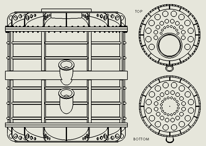
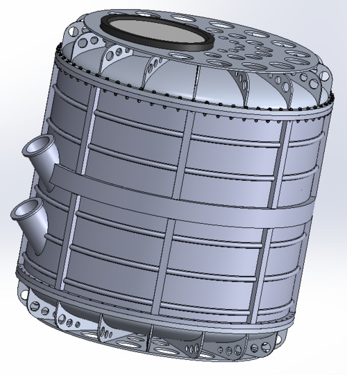
Figure 13: Schematics of the cryostat shell, with outer dimensions indicated, including the two Pulse-Tube heads.

2.2.3 Main Cryostat Cooling System

The cryogenic system is cooled down by two PTs, each providing cooling power of the order of 1W at 4K and 30Wm at 40K.

The two-stages pulse tubes refrigerate two temperature stages: a 40K shield, surrounding the lower temperature stages and intercepting warm radiation loads and supporting low-pass filters on the optical chain, and a 4K stage and shield, surrounding the lower temperature stages, intercepting radiation loads, and supporting directly low-pass filters, the horns array, the wave-plate rotator assembly, and the hexapod of the 1K stage.

A superinsulation blanket is placed between the outer shell and the 40K shield to reduce the radiative load. The two shields are shown in Figure 14 and Figure 15.

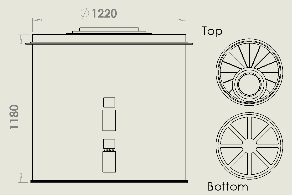
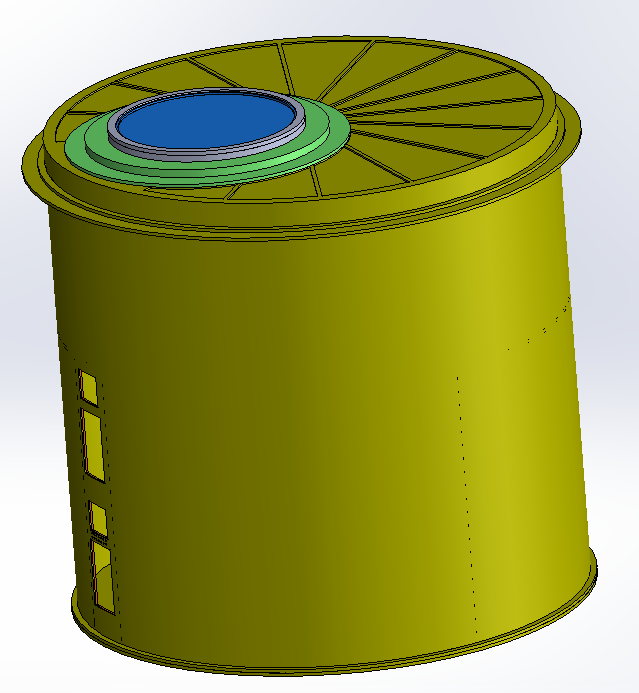
Figure 14: Views of the 40K shield (first PT stage) with main dimensions.

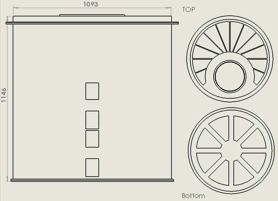
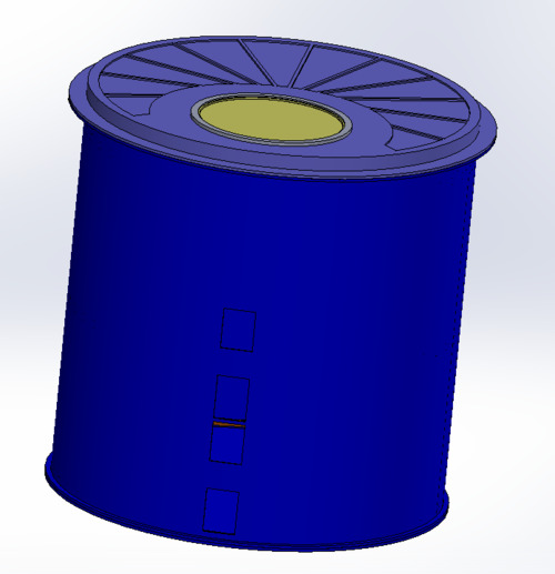
Figure 15: Views of the 4K shield (second PT stage) with main dimensions.

The interfaces between the PTs and the shields, flexible enough to accommodate for differential thermal contraction of the cryostat parts are shown in Figure 16. The key flexible conductive elements are gold-plated copper flaps, optimized for flexibility and heat conduction. Further copper belts are used to thermalize the large shields (especially the 4K one) as shown in the right panel of Figure 16.

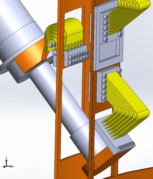
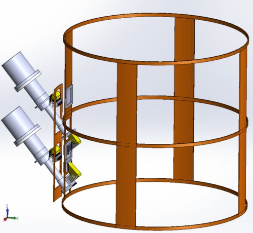
Figure 16: Left: flexible thermal interfaces between the PTs and the shields. Right: system of copper belts used to thermalize the shields.

The 40K stage is held firmly in place by a system of insulating fiberglass tubes assembled as in a drum, as visible in Figure 17. A similar drum is used to hold firmly in place the 4K stage. The support structure is completed by a system of radial fiberglass straps mounted on the bottom of the 40K and 4K shields.

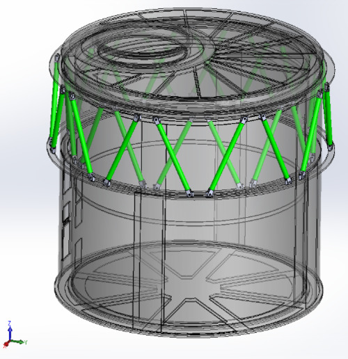
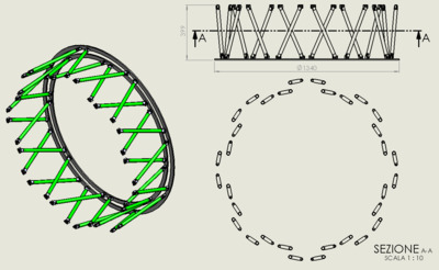
Figure 17: Views of the fiberglass tubes “drum” holding firmly in place the 40K and 4K shields.

Results from a preliminary simulation of the heat loads on the two stages of the system are reported in Table 14.

T1	3.0 K
T2	40 K
T3	300 K
top fiberglass tubes	16
bottom fiberglass straps	6
area of 4K shield	5.81 m${}^{2}$
area of 40K shield	6.12 m${}^{2}$
window diameter	0.50 m
number of superinsulation shields 1-2	10
number of superinsulation shields 2-3	30
number of ASICs	16
W cond (1,2)	91.68	1615.68 mW
W wires (1,2)	0.18	2180.00 mW
W rad window	0.28	901.77 mW
W rad (1,2)	8.43	9369.72 mW
W ASIC (2)		1600.00 mW
Q dot (1,2)	100.58	15667.20 mW

Table 14: Summary of simulated heat loads on 4K and 40K stages.

With a total load of about 0.1W on the 3K stage and of about  16W on the 40K stage, operation with a single pulse tube is possible. We maintain the second pulse tube mainly to handle unexpected large thermal gradients in the system and extra loads from the window and warm filters. Moreover,  when cycling the sub-Kelvin  fridges, operation with a single PT would be marginal. Pre-cooling of the cryogenic sections of the systems is obtained through suitable gas switches.

2.2.4 1K-box

As shown in Figure 18, the 1 K box contains the followings parts:

• The primary and secondary mirrors

• The cold stop

• The dichroic

• The focal plane

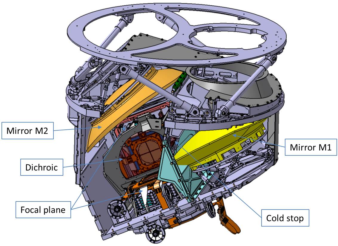
Figure 18: 1K box and its inner parts

The purpose of the 1K box is, on the one hand to assure the mechanical holding and the alignment of these different parts, and on the other hand to ensure a thermal shielding at 1K.

The 1K box is fixed on the 4K stage of the cryostat through its upper support frame (see Figure 19) which will be made of Carbon fiber hexapods (which temperature will thus lie between 4K and 1K). On this upper support frame will also be assembled the horns and switches. The 1K box itself is assembled on its upper support frame by 6 carbon fiber tubes of thin section for thermally insulating the 1K box of the 4K stage of the cryostat. The 1K box will be connected to the 1K subsystem.

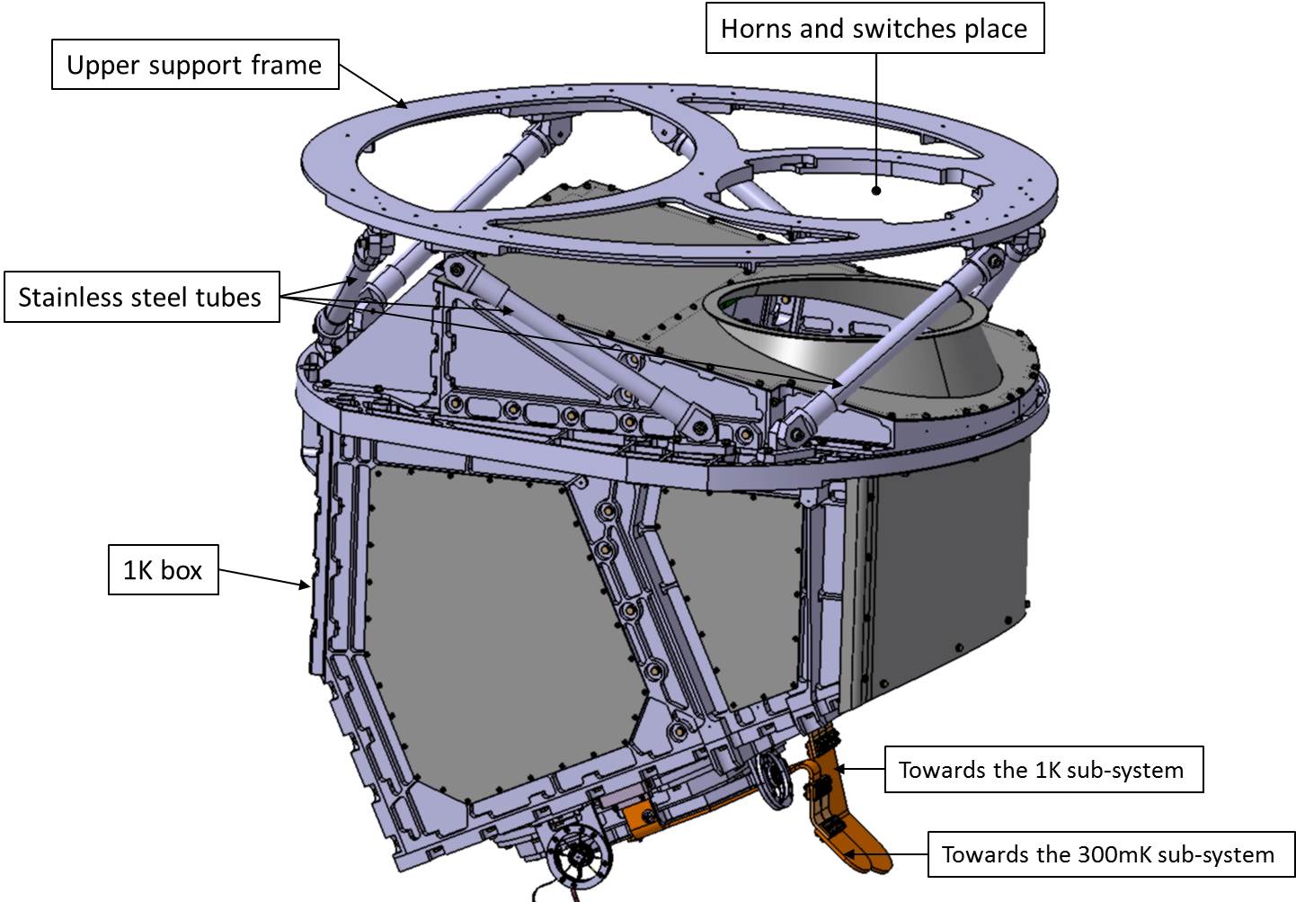
Figure 19: Sketch of the 1K box

The 1K box is made of aluminium alloy sheets and plates with stiffening ribs screwed between them to allow their assembly and to mount and align inner parts (mirrors, cold stop, dichroic, focal plane …). Its design is optimized to reduce its mass (in particular for thermal reason), but also to increase its stiffness. The requirements are that, under the effect of gravity during the displacement of the instrument while scanning the sky, the 1K box must be stiff enough to guarantee the alignment of the optical components, in particular the mirrors and the focal plane. Its dimensions are outlined by Figure 20 and summarized in Table 11.

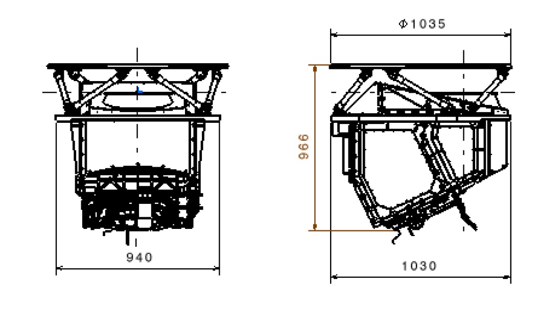
Figure 20: Main dimensions of the 1K box.

2.2.5 1 K System

2.2.5.1 Requirements

This system is dedicated to cool down the optics box from $4.2$ K to $1$ K. Since the requested temperature is in the K-regime, the best option is use an ${}^{4}$He sorption cooler. The optics box is a system of about $165$ kg: $140$ Kg of Aluminium-6061 (Al6061) , $11$ Kg of Stainless Steel 304 (SS304), $10$ kg of Copper and $4$ kg of Brass. In order to support the optics box, there are two possibilities, the first one is the use of Stainless Steel 304 hexapod. Instead, the second one is the use of Carbon Fibre (CF) support. The difference between these two material is mainly due to the thermal load that will be on the optics box. Indeed, the SS304 will introduce a heat load of $168$ J/day at $1$ K, while the CF heat load will be of $43$ J/day at the same temperature. The minimum hold time of the fridge requested for this experiment is one day, plus the time of recycling. In order to cool down from $4.2$ K to $1$ K, the fridge should be able to provide $123$ J. Other contributions (such as radiative transfer from cold environment of from window) can be considered negligible. Indeed, heat load coming from these sources is less than $0.2$ J/day.

A typical ${}^{4}$He sorption cooler is able to provide a minimum cooling power of 2 mW at $1$ K. Considering the latent heat of the ${}^{4}$He, an amount of $1.5$ moles of helium to keep the optics box at $1$ K for an entire day in case of the use of SS304 hexapod with a previous cooling power. While using CF, only $0.55$ moles of ${}^{4}$He are requested. During the cooling phase, a certain amount of gas will evaporate to cool itself. In particular, it is possible to find that the number of moles evaporated is equal to $2.5$ mol for the SS304 support and less than $1$ mol for the CF (This value changes as function of temperature of the pulse tube cold head as it is possible to see in figure 21).

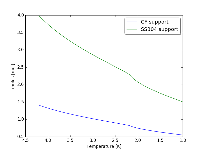
Figure 21: Moles of ${}^{4}$He as function of temperature during the cooling phase.

Therefore, the final requirements for the $1$ K fridge are:

• cooling power of at least $2$ mW,
  

• total time of operation 24 hrs (hold time) plus cooling time,
  

• $4$ mol of ${}^{4}$He using SS304 or $1.5$ mol using CF.

2.2.5.2 Design

To design a fridge that respects the previous requirements, there is the necessity to distinguish the two different solution for the support. In case of the SS304 hexapod, at the moment there is not a fridge able to contain almost $4$ mol, so the easiest way is to design two equal small fridges, each of $2$ mol. Instead in case of CF support, one fridge is enough. A CAD of a single fridge is presented in figure 22. This fridge is designed to reach the requested temperature, and it has been already manufactured, as shown in Figure 23. The condenser of the fridge will be attached to the $4.2$ K flange in order to condense the helium. In addiction to this connection, there will be an heat switch between the cryopump and the $4.2$ K. In order to allow the adsorption of the gas and reducing the temperature of the helium bath, the switch must be in the ON state to cool down the charcoal. When all the gas is adsorbed, a heater will be switched on (and the heat switch off) to increase the temperature of the charcoal up to $50$ K and allows the desorption of the gas. When all the gas is desorbed, the heater will be switched off, so the heat switch on. This phase is very delicate, indeed the charcoal pump will cool down from $50$ to $4$ K releasing a huge amount of energy, some thousands of Joule, on the $4.2$ K flange. This is due to heat capacity, and so the enthalpy difference, of the copper and of the stainless steel that are the main components of pump (in a first instance, it is possible to neglect the heat capacity of the charcoal which is significantly lower). The releasing of this energy will be in a short time corresponding to a power of $2-3$ W, which is greater than the cooling of the pulse tube ($1.4$ W). This means that the $4.2$ K flange will increase its temperature (with a steep spike) and all the other elements attached too. To avoid this problem (which is present in both the cases considered for the support), it is possible to use two different pulse tubes, one of them dedicated only to the ${}^{4}$He fridges (fridge). This implies that only the pulse tube attached to the fridges (fridge) will suffer the temperature drift, while the other components will remain at $4.2$ K thanks to the other pulse tube.

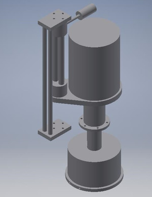
Figure 22: CAD drawings of the 1K Fridge.

2.2.5.3 Testing

The testing phase will start with the commissioning of the new cryostat. This cryostat will use a Gifford-McMahon (GM) mechanical cooler to precool the ${}^{4}$He fridge at suitable temperature to allow the condensation of the gas. The system is presented in figure 23. The sorption cooler will be attached to the cold stage of the GM cooler, which is the lowest copper flange in the picture on le left hand side of Figure 23.

The ${}^{4}$He fridge is presented in figure 23. The indium tube coming from the top of the charcoal pump is visible. This will be connected to a gas line, in this way it is possible to charge, and consequentially test, the fridge with different quantities of the gas.

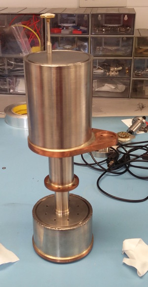
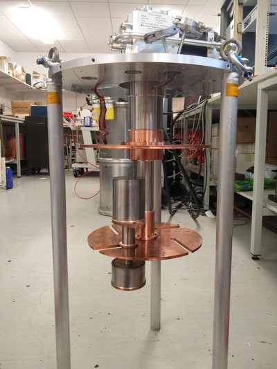
Figure 23: Photo of the ${}^{4}$He Sorption Cooler (left); Photo of the ${}^{4}$He Sorption Cooler mounted on the 4K stage (right).

2.2.6 sub-K systems

2.2.6.1 Sub-K System Description

The ${}^{4}$He + ${}^{3}$He sorption fridge selected to cool the QUBIC focal plane was manufactured by Chase Cryogenics and is shown in Figure 24 (left).It is presently installed within another experiment (cryogenic electron paramagnetic resonance). We are negotiating a calendar for final operations of this system, but for now we have only limited data from earlier tests.

2.2.6.2 Sub-K Performance Tests

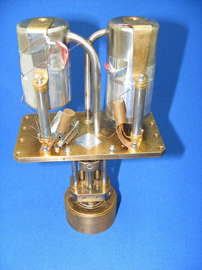
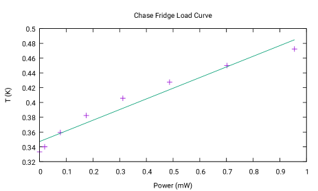
Figure 24: Chase Cryogenics fridge for the focal plane (left), Cold stage load curve for Chase fridge (right)

Figure 24 (on the right) shows a load curve measured with the Chase fridge installed into the EPR system. No loads were connected to the fridge (other than unintentional stray loads, e.g. radiative loading, but we would expect these to be similar).

We do not at this stage have a predicted hold time for the power considered. This fridge has a large charge, however. We will run the fridge with the expected load applied to obtain an expected run-time figure at a later date.

2.2.6.3 Sub-K Interfaces

The fridge requires a certain volume within the system and must be mechanically connected to the 4-K PTC second-stage cold plate and to the focal plane attachment. A crude CAD model of the fridge has been provided. When we have full access to the fridge again we will verify the dimensions of these mechanical interfaces.

Heat will flow into the fridge from the focal plane attachment and from the fridge to the 4-K plate. The heat lift from the FP will be characterized as described above. The energy flow to the 4-K stage will be substantial. This is illustrated by Figure 25, which shows the response of the 2nd stage of a Sumitomo RDK415 GM cooler from 3 cycles / part cycles of the Chase fridge. Admittedly no particular effort has been made to be gentle with these cycles, but the peak temperature of 7 K corresponds approximately to a peak load of 7 W. For sure careful operation of the fridge can reduce this, perhaps by a factor of two.

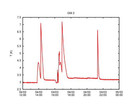
Figure 25: The effect on GM cooler 2nd-stage T from operation of the fridge

Type	Location	No. Wire Pairs	Notes
Diode	${}^{4}$He heat switch	1
Heater	${}^{4}$He heat switch	1
Diode	${}^{3}$He heat switch	1
Heater	${}^{3}$He heat switch	1
Diode	${}^{4}$He cryo pump	1
Heater	${}^{4}$He cryo pump	1
Diode	${}^{3}$He cryo pump	1
Heater	${}^{3}$He cryo pump	1
RTD	Cold stage	2	Optional
RTD	Intermediate stage	2	Optional
Heater	Cold stage	1	Optional

Table 15: Sub-K fridge electrical interfaces

The operating conditions of the heaters will be confirmed later, but are 25 V max 100 mA max. Currently we are using 0.1-mm copper twisted pair to supply power to the heaters, but in the past we have used 0.1-mm Manganin.

Operation of the fridge will require readout of the cold stage temperature. This could be a thermometer mounted as close as possible to the cold stage for this purpose. However, a thermometer elsewhere on the load should be adequate. A thermometer on the intermediate stage can be useful.

A heater on the cold stage can be useful for verification of fridge operation (load curves) or warming up the system. It could also be used for thermostatic control. However, it is not vital.

Currently a micro-D connector is mounted to the fridge for these connections. Gender and pin-out will be confirmed at a later date.

The readout of the thermometers can be by typical equipment (e.g. Lakeshore 370, 318). We use computer-controlled heaters capable of driving up to 25 V at 100 mA.

Our in-house control system uses an xml script to describe a state machine for fridge cycling. For example, one state might set heat switch drive Voltages, with a test condition that would progress to a timed wait state once both heat switch thermometers are reading a high enough temperature. This script should easily translate to whatever control system is employed.

2.2.6.4 Sub-K Verification

Tests as described in section 2.2.6.2 have been conducted to check for adequate hold time at the expected power, the results are summarized in tables 16 and  17.

$P_{\hbox{load}}$ ($\mu$W)	Days	Hours	Seconds	Joules	T (mK)
19.5	3.75	89.92	323700	6.31	336 mK
43.9	2.45	58.83	211800	9.29	349 mK

Table 16: ${}^{3}$He hold times for two load values.

$P_{\hbox{load}}$ (mW)	Days	Hours	Seconds	Joules	T (K)
4.39	0.03	0.70	2520	11.05	1.2 K

Table 17: ${}^{4}$He hold times for one load value.

2.2.6.5 Transportation Issues

It should be noted that this fridge (and the 1-K fridge) relies upon thin-walled tubing to contain high-pressure gas. This makes it necessary to take extra precautions whilst shipping. The fridge will be shipped from Manchester with any shipping stays considered necessary, and comparable arrangements must be put in place to stiffen the assembly sufficiently for onward shipping after integration.

2.2.7 Heat Switches

2.2.7.1 Heat Switches Description

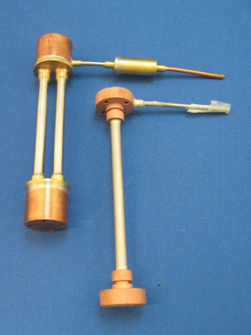
Figure 26: Both switch types

For the base-line configuration two types of heat switch are considered (see Figure 26):

Convective Heat Switch

Two thermal stages (OFHC copper) are connected with a twin-pipe circulation system (thin-wall stainless steel). Helium is injected into the circuit using a small cryo pump. So long as the physically-higher stage is colder than the lower stage the gas will convect around the circuit. Gas is cooled by the upper stage and warmed by the lower stage, effecting a transfer of heat. If the switch is operated across a phase transition (i.e. the stages are above and below the boiling point) heat transfer is especially effective due to the latent heat taken / given up by condensing / boiling.

Minimal Gap Heat Switch

This new design uses a single stainless-steel tube, which is almost filled with a copper rod, with a small gap around the rod such that it is not in contact with the inside wall of the tube. This is not connected to the bottom, but at room temperature it might just touch the bottom stage. At cryogenic temperatures differential contraction opens a very small gap at the bottom of the rod. This means that the off conductance will be determined solely by the conductance of the stainless steel tube. Helium from a cryo pump (not fitted in the photo) is released into the volume to turn the switch on. Conduction across the small gap by helium gas is very effective. When the low end temperature is low enough to condense liquid to bridge the gap the conductance rises further, and further still with the formation of super-fluid helium.

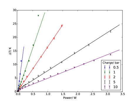
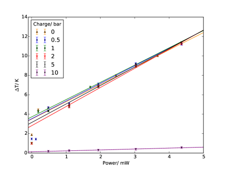
Figure 27: Heat switch on (left) and off(right)

We use convective switches routinely, for example to cool large sorption-fridge cryo pumps. In fact the example presented here has been designed for use with the large ${}^{4}$He fridge we propose for cooling the 1-K Box. This design uses larger tubes than previously for higher heat transport. For use at lower temperatures where the off resistance should be optimized we would probably choose finer tubes.

2.2.7.2 Heat Switch Performance Tests

Results from on and off conduction measurements of the convective switch are given in Figure 27 on the right and left hand side respectively (note the different power scales). These were taken with a range of ${}^{4}$He charge pressures. As may be anticipated increasing the charge results in higher heat transport. However, the 10-bar charge clearly shows that the off conductance has been compromised. We intend to repeat this test with a larger cryo pump.

Whilst we have not made a test with a negative temperature difference imposed on the switch we would expect the residual conductance to be, at worst, no more than the y-intercept of the off measurements. We would expect a reduction in practise, since whilst an residual vapour can contribute heat transport by convection when the bottom stage is warmer than the top, with the bottom stage now held cold than the top this should be suppressed.

Our tests of the minimal-gap arrangement have so far been unsatisfactory. We will report further as this develops. We expect to be able to provide adequate conductance with the convective switch if the MGHS is unsuccessful.

2.2.7.3 Heat Switch Interfaces

The mechanical interfaces to the heat switches are the 4-hole mounting points at top and bottom. Correct orientation is paramount, with the item to be cooled attached to the lower stage. The height of the switches is to-be-decided. The volume taken by the switch may be inferred from the CAD model. There is some flexibility in terms of reorienting the cryo pump, but note that we might want to double the size over that shown in the model. A weak link wire will be required to bring the cryo pump to 4 K.

Thermally, the switch will accept thermal power at the bottom and couple it to the top. The load on the fridge will be determined mostly by the power extracted from the cooled stage. A small amount of power is added by the cryo pump.

Electrical interfaces are described in table 18. Provision of thermometers / heaters has not been discussed. The type preferred elsewhere may be used for the switch, for operation from room temperature to 4 K. The maximum power to the heater is typically less than 500 mW (actually more usually about 200 mW) but up to a few W can be useful when a rapid heating is desired. We use 330R, max 32 V 100 mA with 0.1-mm copper wire (but we have used 0.1-mm Manganin in the past).

Type	Location	No. Wire Pairs	Notes
Diode	Heat switch cryo pump	1
Heater	Heat switch cryo pump	1

Table 18: Heat switch electrical interfaces (per switch)

As for the fridge our usual computer control uses a state machine language. Operation of a heat switch is trivial and this approach may readily be translated to the language of choice.

2.3 Optical chain

As shown in Figure 2, the sky radiation experiences several steps as it propagates through the optics of the QUBIC 1^st module; all of them are described in this section.

The optical chain shown on Figure 28 is completed with a selection of spectral conditioning before the combiner : in intensity, by filters, and in polarization, by a modulator (HWP) and a polariser. A dichroic, before the focal planes, splits the radiation into the two bands at 150 and 220 GHz. Finally a couple of radiation shields in front of the cryostat and around the whole instrument allow a reduction of local spillover.

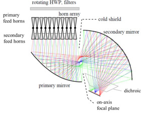
Figure 28: The off-axis dual reflector chosen for the QUBIC beam combiner. The rays, at -7°(green), 0°(blue) and +7°(red) represent the beams from the re-emitting horns.

2.3.1 Window

The window is the first optical element encountered by the incoming radiation beam, and separates the high vacuum present in the cryostat jacket from the room-pressure environment, while allowing millimeter waves in the cryostat. A cylindrical slab (560 mm diameter, 20 mm thick) of high-density polyethylene (HDPE) has been used, as the best compromise between transparency at mm waves and stiffness (the window must withstand an inward force of about 2.4 tons due to atmospheric pressure).

The HDPE slab is pressed against the top cover of the cryostat by an Al ring (see Figure 29) with a suitable number of screws. The vacuum seal is obtained using an elastomer o-ring for laboratory tests, and an indium seal for operation in Concordia, at very low ambient temperatures. The pressing ring is designed to mitigate the effects of differential thermal contractions, which is significant for HDPE vs aluminum.

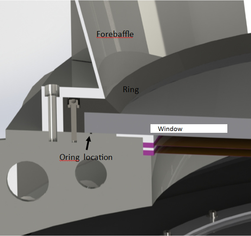
Figure 29: Detail of the window mounting system.

2.3.2 Half Wave plate

2.3.2.1 Mesh Half Wave plate

The QUBIC mesh HWP is designed to work across the two bands of the QUBIC first module instrument (see Figure 19). This means that good RF performance needs to be achieved across a large relative bandwidth, of the order of 73%. The required diameter is 500mm clear aperture.

Table 19: Mesh-HWP bandwidth requirements.

Channel	$\nu_{1}$ (GHz)	$\nu_{2}$ (GHz)	Bandwidth
150 GHz	127	171	30%
220 GHz	192	272	34%
2 channels	127	272	73 %

The QUBIC HWP is based on metamaterials (Figure 30). These devices are alternative solutions to the more massive, expensive and limited-diameter birefringent Pancharatnam multi-plates. The metamaterials are developed using the embedded mesh filters technology. Very large bandwidth mesh-HWPs ($\approx 90\%$) have been successfully realised in the past. They have been used for millimetre wave astrophysical observations at the 30m IRAM telescope with the NIKA and NIKA2 instruments[NIKA2]. The measured performance of a typical prototype, in terms of transmissions and cross-polarisation, are reported in Figure 31 which shows a very good agreement between model and data.

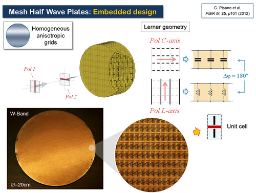
Figure 30: Embedded mesh-HWP based on metamaterials.

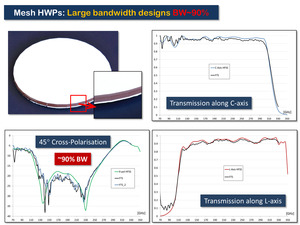
Figure 31: Large bandwidth (~93%) mesh-HWP prototype: modeled and measured performance.

The QUBIC final design is very similar to the prototype discussed above. The bandwidth requirements are less challenging and this allows to achieve better in-band RF performance. The design is based on 12 anisotropic mesh grids and the overall thickness is of the order of 3.5mm. The expected performances of the QUBIC mesh HWP are reported in Figure 32. The averaged transmissions, absorptions, differential phase-shift and cross-polarization are listed within the same figure.

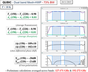
Figure 32: Expected performance of the QUBIC broadband mesh-HWP design.

2.3.2.2 Rotational system for the HWP

Polarization modulation is achieved by rotating a large diameter HWP (Half Wave Plate). Since the HWP is mounted on the 3K stage of the cryostat, a cryogenic rotation mechanism is needed. The one designed for QUBIC inherits several of the solutions developed for cryogenic rotator developed for the PILOT balloon-borne instrument successfully flown by CNES[salatino2] This is a stepping rotator, able to position the HWP in 8 different positions, in steps spaced by 11.25°, for redundant coverage of the needed position angles. The system is shown in Figure 33. The HWP is rotated by a stepper motor mounted outside the cryostat shell. Motion is transmitted through the shell by means of a magnetic joint. A fiberglass shaft transmits the rotation to the cryogenic part of the system, with negligible heat load, and rotates a pulley driving a Kevlar belt. The HWP support ring has a groove for the Kevlar belt, which is tensioned by a spring-loaded capstan pulley. The HWP support ring is kept in place by three spring loaded hourglass shaped pulleys at 120°, as shown in Figure 33. All the pulleys rotate on optimized-load thrust-bearings for minimum friction. The step positions of the HWP are set by holes sets precisely located on a section of the HWP support ring: this builds a 3-bits optical encoder read by optical fibers (see [salatino2] for more details).

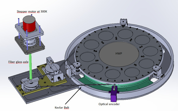
Figure 33: General view of the cryogenic waveplate rotator.

The HWP is mounted on the ring by using a custom made block in order to reduce the differential thermal contraction between Al and Polyethylene (see Figure 34).

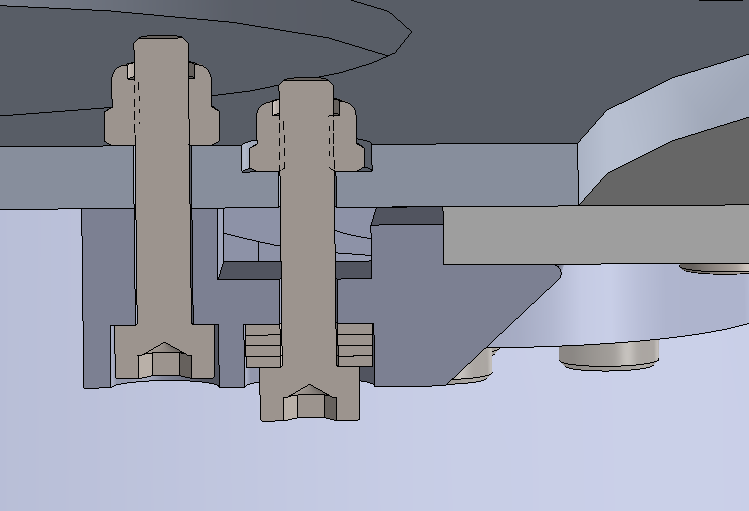
Figure 34: Detail of the HWP clamp.

2.3.3 Filters / Polarizer /Dichroïc

The general philosophy in filter provision is two-fold: 1. To minimise the thermal loading at the various temperature stages by sequentially rejecting short wavelength radiation. This is achieved with thermal filters in combination with baffling and careful optical design, to ensure that the out of band and thermal load at the detector arrays is suitable for the scientific requirements. 2. To define the required spectral passband at the arrays and maximise the in-band optical transmission. There will be an optimization procedure on the entire filter chain to maximise transmission (i.e. to manage the relative fringing between filters) and minimise out-of-band radiation. In addition the filters must be able to withstand cryogenic cycling and maintain flatness within their mounts These specifications have been proven in the past with the AIG’s strong heritage in space mission filter production (e.g. ISO, Mars observer, Cassini, Herschel & Planck Space Observatories) and with ground-based instruments, such as SCUBA2, BICEP and SPT. The QUBIC development puts in place the need for larger diameter components than the AIG have previously provided.

2.3.3.1 QUBIC optical configuration

The QUBIC instrument optical layout/cryostat design is shown in Figure 28. A series of band-defining, blocking and thermal (IR) filters will be mounted at different temperature stages, with a large photolithographic polarizer and a single rotating mesh HWP at 6K We have allowed provision for a high number of filters at critical apertures and temperatures, although these may later prove unnecessary.

2.3.3.2 Mesh Filter Specification

The complete list of devices to be supplied by Cardiff University to QUBIC is given in Table 20.

Table 20: Metal mesh devices to be supplied by Cardiff University to the QUBIC project. Z coordinates are given in the Global Reference Frame (GRF). (*) emissivity could be lower. (**) low frequency in reflexion, high frequency in transmission.

Component	Temp	Transm	Emissivity	Coord. Z GRF	Optical diameter	Useful diameter
	K	$\%$	$\%$	mm	mm	mm
Common to 2 bands
Window	250	98	1	480.00	407	600
IR blocker 1	250	98	1	460.00	401	600
IR blocker 2	250	98	1	452.55	401	600
IR blocker 3	100	95	1	342.10	385	430
IR blocker 4	100	98	1	335.00	381	430
IR blocker 5	100	98	1	327.10	381	430
IR blocker 6	6	98	1	285.50	371	410
12cm-1 LPE	6	95	2	276.30	371	410
HWP	6	95	2.5	237.80	361	380
Polarizer	6	99	1	183.60	352	380
B2B horns + switches	6	99	5	0.0	330	(*)
Beam combiner	1	99	<1
Cold stop 10cm-1 LPE	1	95	2			Ellipse 0.26 x 0.3
Dichroic filter	1	95	2			Ellipse 0.253 x 0.482 (**)
Band1: 150 GHz Singlemoded
6cm-1 edge	0.3	98	2
8cm-1 LPE	0.3	98	2
						$\oslash$maxi = 0.11486
Band2: 220 GHz Multimoded (bandpass 200-240 GHz)
9cm-1 edge	0.3	98	2
11cm-1 LPE	0.3	98	2
Band defining filters	0.3	80	2			$\oslash$mini = 0.1036
						$\oslash$maxi = 0.11486

2.3.3.3 Mesh Filter QO deliverables

IR Blocking filters
Up to 500mm active thermal filter devices are required of 2 or 3 basic pattern types. The transmission performance of prototype (300mm) devices is given in Figure 35. These thermal filters are single layer metal-mesh element devices that reflect a high proportion of the unwanted IR radiation. They require a simple aluminium support ring and the filter element itself is only 4$\mu$m thick.

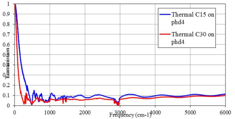
Figure 35: Transmission performance of thermal filters for the QUBIC instrument.

Blocking Filters (Low Pass Edges) - 6K, 1K, 0.3K stages Throughout each optical chain there will be a series of 4 low-pass edge filters per band/pixel. These will be located at the 6K and 1K stages and at the 320 mK array. These are designed to block out-of-band FIR radiation, whilst maintaining high in-band throughput. The transmission performance of the 3 possible large low-pass elements common to both bands is given in Figure 36. Although, for the purposes of all large scale CMB instruments, we have recently prototyped a new, multi-element 12cm${}^{-1}$ LPE filter which will have improved FIR rejection (1 part in 104) - see Figure 37.

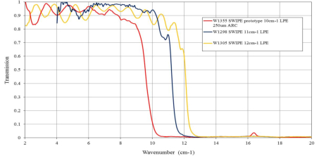
Figure 36: Transmission performance of prototyped common LPE blocking filters

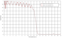
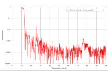
Figure 37: Transmission performance of possible 12cm${}^{-1}$ blocking filter.

The thickness of these current filter elements is as follows:

• 10cm${}^{-1}$ LPE 1.4mm without ARC, 1.8mm with ARC;

• 11cm${}^{-1}$ LPE 1.3mm;

• 12cm${}^{-1}$ LPE 2.2mm;

Band Defining Filters - 150, 220 GHz
Band-defining filters are required at 150 and 220GHz:
150 GHz is single-moded with a band-edge at 5.6 cm${}^{-1}$ (25% BW)
220 GHz is multi-moded with 18% bandwidth, requiring a band-pass filter or a high-pass low-pass combination (6.7 $cm^{-1}$ - 8.0 $cm^{-1}$).

Typical filter performance for a number of 150/220GHz options, with modelled atmosphere is given in Figure 38.

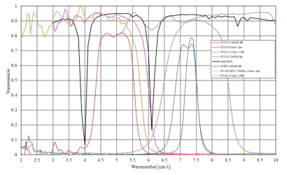
Figure 38: Transmission performance of possible 12cm${}^{-1}$ blocking filter.

Dichroic
This filter is designed to transmit (>90%) the 220GHz band, whilst reflecting (>90%) the 150GHz band. Prototype hot-press and air-gap 6.5 cm${}^{-1}$ HPE devices have been produced by Cardiff AIG and shown to be effective in both reflection and transmission at up to o°incidence. Figure 39 show normal incidence transmitted performance.

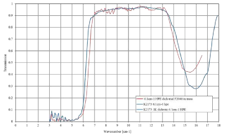
Figure 39: Transmission performance of a prototype 6.5cm${}^{-1}$ high-pass dichroic in airgap (red) and hot-pressed (blue) options

Further testing of prototype devices is underway, with emphasis on the mounting and flatness fo these large components. A hot pressed device will be the preferred option, provided that the R and T performance are found to be comparable to that for an air-gap device and that flatness can be maintained through cryogenic cycling.

Photolithographic polarizer
A 10$\mu$m period wired polarizer is required for 6K operation. A prototype has been made at 450mm diameter. This is shown in Figure 40.

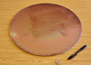
Figure 40: Example previously manufactured large diameter polariser (45cm diameter).

2.3.3.4 Quasi-Optical component fabrication, assembly and tests

All the Quasi-Optical (QO) components (mesh filters, half-wave plate, polarizer and dichroic) are manufactured by the Astronomy Instrumentation Group (AIG) in Cardiff. This group is the largest manufacturer and first world supplier of metal-mesh components. Devices from this group have been successfully used in tens of astronomical experiments ranging from ground-based to satellite missions.

The QO components are manufactured by using photolithographic techniques, specifically the mesh-technology. The TRL level is 9 for mesh-filters, polarizers and anti-reflecting (ARC) coatings. Mesh-HWPs have been successfully used recently in ground-based experiments.

The devices will be completely built within the cleanrooms of the Cardiff AIG. All the grids for all the device will be visually checked. In addition, dimensional measurements will be required during the mesh-HWP development due to the criticality associated to the phase response of each grid. The assembly and the bonding of the grids will be carried out within our cleanrooms.

Depending on the type of device and on their thickness, different types of mechanical mounts will be used for the different components. These metallic rings will guarantee rigidity, flatness and operation at cryogenic temperatures.

The filters, the HWP, the polarizer and the dichroic will all be tested and characterised in our laboratories by means of different Fourier Transform Spectrometers. Different experimental setup will be adopted for each type of device.For example, the HWP tests will require transmission measurements along the two axes and cross-polarisation at 45 degrees rotation angle. The frequency range of the tests will cover the QUBIC operational bandwidth. For the thermal filters, the measurements will be extended up to the near-infrared region to check for unwanted leakage.

2.3.4 Horns

Similarly to the switches, we have been through a prototyping campaign of the QUBIC feed horn array.

This array is composed by two blocks of 400 horns each. The two blocks are placed back-to-back with a layer of switches that can open or close the optical path to the radiation (cf. previous section and section LABEL:operation).

The feeds are corrugated horns optimized for a wide-band response (in the range 130-240 GHz). They are based on a modification of a previous design, which was optimized for 150 GHz only, when QUBIC was still designed for 150 GHz-only measurements. The left panel of Figure 41 shows the current profile of the QUBIC horns; we call this the QUBIC2 design. The right panel shows the original design adopted for the 150 GHz – only version of QUBIC; we call this the QUBIC1 design.

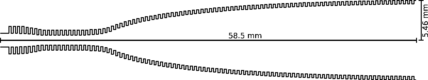
Figure 41: Left panel: the current design of the QUBIC feed horns, optimized for wide band response. Right panel: the first design of the QUBIC feed horns, optimized for 150 GHz measurements.

2.3.4.1 2x2 prototypes array

The manufacturing of several horns with complex internal geometry with sub-mm tolerance is a challenging task. To achieve the result we identified the platelet technique as the most suitable to build such a large array with affordable cost. According to this technique the horn is built from suitably drilled metal platelets that are subsequently stacked to form the horn structure.

For QUBIC, we chose Photochemical Etching and Milling to drill the platelets. This technology is applied to a wide range of materials for the fabrication of highly complex objects, with an achievable precision of the order of ± 10% the material thickness.

To verify the applicability of this technology to QUBIC horns we set up a prototyping campaign with the following objectives:

• Verify the possibility to manufacture the horns and assess the achievable mechanical tolerance,

• Assess the electromagnetic performance of the obtained horns in terms of return loss, insertion loss and angular beam pattern and compare it with the simulations,

• Verify the scalability of this technique to a large number of elements.

In this prototyping phase we built 6 prototypes, which are detailed in Table 2.3.4.1.

Prototype n.

128 (two 8x8 modules)

QUBIC2

Silver-plated anticorodal

Check of manufacturing scale-up Verification of interface with switches Verification of feed-switch functionality

In progress

Table 21: List of QUBIC feed horn array prototypes

In Figure 42 and Figure 43 we show pictures of the QUBIC1 brass prototype, which has been cut to perform a visual inspection of the corrugation details.

Figure 43, in particular, shows details of the inner structure of the feed corrugations, revealing the presence of small cusps on the top of each tooth and groove. These features likely result from a non-homogeneous action of the chemical agent on the metal.

We have analyzed with simulations the impact of such defects on the feed-horn performance and the result is that the impact is negligible. This analysis is presented in Section 2.3.4.2

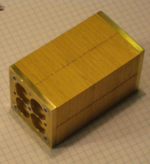
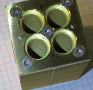
Figure 42: Outer view of the brass QUBIC1 prototype.

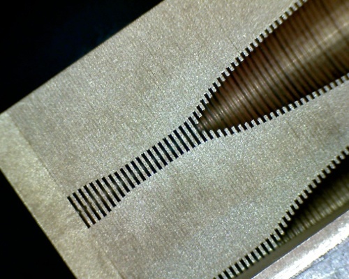
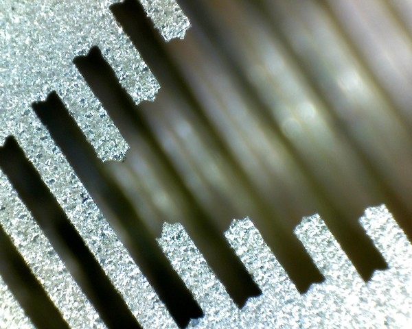
Figure 43: Inside view of the brass QUBIC1 prototype. Left: Cusp in groove. Right: Cusp on tooth.

In Figure 44 and Figure 45 we show the complete set of 2x2 prototypes.

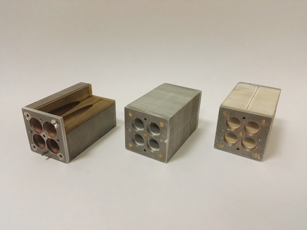
Figure 44: Brass prototype (left), anticorodal prototype (middle), silver-plated anticorodal prototype (right).

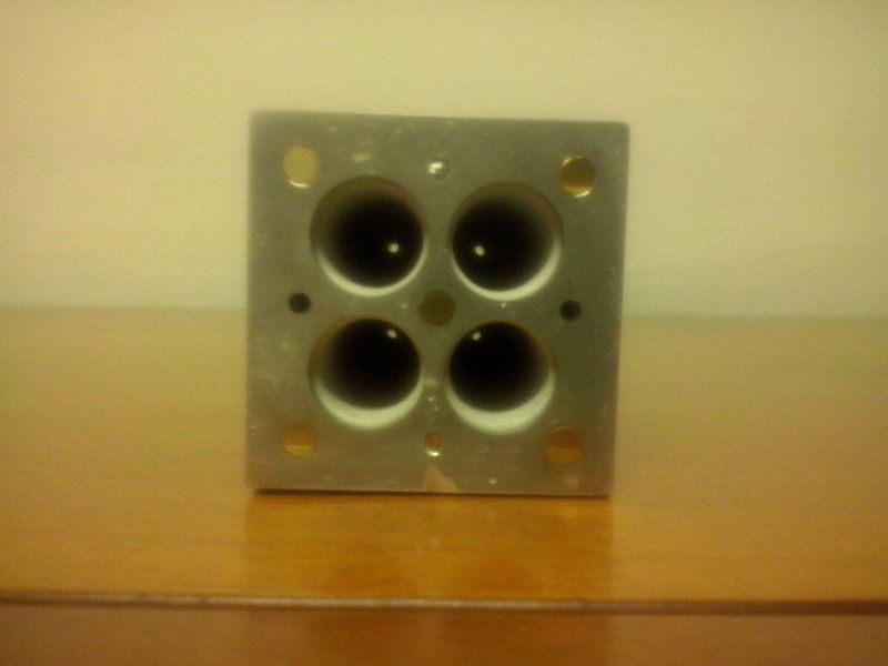
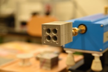
Figure 45: QUBIC1 aluminum prototype (left), QUBIC2 anticorodal prototype (right).

2.3.4.2 Metrological measurements

Here we report the results of metrological measurements performed on the platelets of the brass module prior to its integration. We measured the diameters of the antenna holes with a Werth Scopecheck 200 metrological machine and compared measurements with the nominal values in the mechanical drawing. More details are given in Figure 46 which shows the absolute and relative deviations of the measured diameters with respect to the nominal one as a function of the diameter itself. From these results we can draw the following considerations:

1. The relative error is approximately constant, of the order of 0.5% or less, apart from diameters smaller than $\approx$2 mm, for which the relative deviation is of the order of 1%

2. There is a systematic trend: smaller holes tend to be larger than the nominal, larger holes tend to be smaller. This trend could be in principle corrected in the manufacturing if necessary by correcting the drawings.

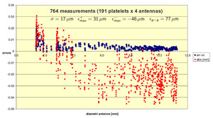
Figure 46: Absolute and relative deviations of measured diameters with respect to the nominal ones as a function of the diameter. The plot shows a systematic trend in these deviations that remain, however, at a level less than 1%.

Figure 47 shows the deviation of the measured position of the holes center from its nominal value. We see that the distribution of these errors is not symmetrical around the origin but lies preferentially along one direction. This asymmetry can be mitigated during integration, by turning every other plate by 90°.

We see that the r.m.s. values of these deviations are in the range 10 – 20 µm, so about two order of magnitudes less than the wavelength. Therefore we expect that they will not impact the electromagnetic performance of the feed significantly. This is confirmed by our return loss measurements reported in Section LABEL:bkm:Ref435184286.

Figure 47: Deviation of the hole center position with respect to the nominal value. The distribution of these deviations is asymmetrical. This asymmetry can be mitigated during integration by turning every other plate by 90°.