Detection of a $\sim$20 kpc coherent magnetic field in the outskirt of merging spirals: the Antennae galaxies

Abstract

We present a study of the magnetic field properties of NGC 4038/9 (the ‘Antennae’ galaxies), the closest example of a late stage merger of two spiral galaxies. Wideband polarimetric observations were performed using the Karl G. Jansky Very Large Array between 2 and 4 GHz. Rotation measure synthesis and Faraday depolarization analysis was performed to probe the magnetic field strength and structure at spatial resolution of $\sim 1$ kpc. Highly polarized emission from the southern tidal tail is detected with intrinsic fractional polarization close to the theoretical maximum ($0.62\pm 0.18$), estimated by fitting the Faraday depolarization with a volume that is both synchrotron emitting and Faraday rotating containing random magnetic fields. Magnetic fields are well aligned along the tidal tail and the Faraday depths shows large-scale smooth variations preserving its sign. This suggests the field in the plane of the sky to be regular up to $\sim 20$ kpc, which is the largest detected regular field structure on galactic scales. The equipartition field strength of $\sim 8.5~{}\mu$G of the regular field in the tidal tail is reached within a few 100 Myr, likely generated by stretching of the galactic disc field by a factor of 4–9 during the tidal interaction. The regular field strength is greater than the turbulent fields in the tidal tail. Our study comprehensively demonstrates, although the magnetic fields within the merging bodies are dominated by strong turbulent magnetic fields of $\sim 20~{}\mu$G in strength, tidal interactions can produce large-scale regular field structure in the outskirts.

1 Introduction

Magnetic fields are pervasive in the Universe on all scales and they play crucial roles in various processes in the interstellar medium. The large-scale ordered magnetic fields ($\gtrsim 1$ kpc) in galaxies are thought to be amplified via the $\alpha$–$\Omega$ dynamo mechanism—the buildup of initially weak seed fields ($<10^{-9}$ G; Ade et al. 2015) to microgauss fields via small-scale turbulence and differential rotation (Ruzmaikin et al., 1988; Kulsrud & Zweibel, 2008). The small-scale dynamo can efficiently amplify the magnetic fields on scales $\lesssim 1$ kpc in $\sim 10^{6}$ years (Subramanian, 1999; Federrath et al., 2011; Chamandy et al., 2013; Schober et al., 2013). On the other hand, the conventional $\alpha$–$\Omega$ dynamo action requires $\sim 10^{9}$ years to amplify the large-scale magnetic field in galaxies (Arshakian et al., 2009; Pakmor et al., 2014), which is too long to explain the detection of coherent fields in young systems (e.g., Bernet et al., 2008; Farnes et al., 2014). This suggests that there must be other magnetic field amplification processes at work.

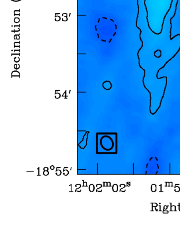
Figure 1: Left-hand panel: Total intensity image of the Antennae made by combined DnC+CnB array data at a centre frequency of 2.8 GHz having angular resolution $11\times 9$ arcsec². Overlaid are the contours at [$-3,-2,3,6,12,24,50,75,100,150,200,350,500$] $\times 40~{}\mu$Jy beam^-1 levels. The dashed contours represents negative total intensities. Right-hand panel: We label the various regions in NGC4038/9 that are studied in the paper on the HST-F658N narrow-band filter image tracing the H$\alpha$ emission of NGC 4038/9 with total radio continuum intensity contours shown same as the left-hand panel.

In the current framework of hierarchical structure formation, galaxies build up their mass by merging. Galaxy encounters can compress, stretch and reshape fields in the progenitor galaxies, hence they provide a conducive environment for magnetic field amplification (Kotarba et al., 2010). Since merger events were more frequent in the early Universe (e.g., Patton et al., 2002), it is important to assess how galaxy interactions affect the strength and geometry of galactic-scale magnetic fields in order to understand the overall evolution of cosmic magnetism. Gravitationally interacting galaxies possess a range of magnetic field properties. For example, despite their irregular appearances, the tidally interacting Magellanic Clouds have been shown to host large-scale ordered fields of microgauss strength (Gaensler et al., 2005; Mao et al., 2008, 2012). On the other hand, Drzazga et al. (2011) suggested, based on study of 16 merger pairs, that interacting galaxies have lower field regularities and stronger total magnetic field strengths than non-interacting ones. Unfortunately, due to the lack of Faraday rotation measure (RM) information, the magnetic field coherency in these systems could not be probed. Moreover, the large distances to their sample galaxies and the limited angular resolution prevent one from studying magnetic field structures on scales $<7$ kpc. Therefore, a high resolution mapping of the magnetic field of a prototypical merger event is much needed. To date, detailed high-resolution studies of galactic magnetic fields are of individual galaxies in isolation—only a few focus on magnetism in interacting galaxies (e.g., Brindle et al., 1991; Hummel & Beck, 1995; Chyży & Beck, 2004; Rampazzo et al., 2008).

The Antennae pair (NGC 4038/9) is the nearest merger (22 Mpc; Schweizer et al., 2008) between two gas-rich spirals. The bodies of the colliding galaxies host sites of active star formation in the form of super starclusters, with a global star formation rate of 20 M_⊙ yr^-1 (Zhang et al., 2001). The Antennae galaxies hosts tidal tails that measure over 100 kpc in Hi and likely originate from outskirts of the progenitors. The Antennae have been studied extensively from the radio to X-ray. They are also the subject of several numerical simulations (e.g., Mihos et al., 1993; Karl et al., 2010; Kotarba et al., 2010). The latest work by Karl et al. (2010) proposed that the progenitors first encountered $\sim 600$ Myr ago and they have just undergone the second passage. Our understanding of the pairs’ interaction history, its multi-wavelength emission and its proximity make the Antennae an ideal candidate for a detailed magnetic field study.

Magnetism in the Antennae was studied by Chyży & Beck (2004) with the Very Large Array at 1.49, 4.86 and 8.44 GHz. Enhanced polarized emission is found near the root of a tidal tail which is suggestive of a remnant spiral field. Chyży & Beck (2004) computed the RM of diffuse polarized emission at 8.44 GHz and 4.86 GHz at a resolution $17\times 14$ arcsec² ($\sim 2$ kpc linear scale). They pointed out that in the region where the galactic discs overlap, RMs are coherent on the scale of several synthesized beams, likely tracing the large-scale magnetic fields in the progenitors. There are several regions with consistent RM sign, which is suggestive of coherent magnetic fields. However, these RMs could suffer from the $n\pi$ ambiguity because they were computed using polarization angle measurements at only two bands, separated widely in frequency. A wideband study of the diffuse polarized emission from the Antennae is much needed to consistently derive RM to confirm the existence of coherent magnetic fields.

In this paper, we present study of the magnetic field properties in the Antennae galaxies. In §2, we describe our observations and data analysis procedure. The results on Faraday depolarization and magnetic field strengths are presented in §3 followed by discussion in §4. Our results are summarized in §5.

2 Observations and analysis

We carried out wideband polarimetric observations of the Antennae galaxies using the Karl G. Jansky Very Large Array (VLA) in the hybrid DnC array configuration on 10-May-2013 and CnB array configuration on 09-September-2013 (project code: 13A-400). Data between 2 and 4 GHz (divided into 1024 2-MHz channels) were recorded with the widar correlator. The 1024 channels were divided in 16 sub-bands known as spectral windows. Two scans of 15 minutes each using the DnC array and 30 minutes each using the CnB array on the Antennae were interspersed with $\sim 3$ minute scans on the phase calibrator J1130$-$1449. 3C 286 was observed as the flux, bandpass and absolute polarization angle calibrator for 10 minutes at the beginning of each observation run. Unpolarized point sources, J0713$+$4349 and J1407$+$2827, were used to calibrate polarization leakages. We used the Perley & Butler (2013a) flux density scale to determine the absolute flux density of the flux calibrator 3C 286 and its absolute polarization angle was set to $+33^{\circ}$ across the entire observing band (Perley & Butler, 2013b).

Data reduction was carried out using the Common Astronomy Software Applications (casa) package following standard data calibration procedure for each array configuration separately. The task ‘rflag’ was used to automatically flag data affected by radio frequency interference (RFI). Further manual inspection of the data was done to remove low-lying RFI features. Overall, for both array configurations, approximately 750 MHz of data were unusable and the remaining $\sim 1200$ MHz of data (non-continuous, spanning between 2 and 3.6 GHz) was used for further analysis. Several rounds of calibration and additional flagging were done iteratively, and the gain solutions were transferred to the target source. To estimate the on-axis polarization leakage post calibration, we made a linearly polarized intensity ($PI$) image of the unpolarized calibrator J0713$+$4349. The image was consistent with noise throughout. We estimate the on-axis instrumental polarization leakage as the ratio of the maximum value of the $PI$ image at the position of J0713$+$4349 to its total flux density, which was found to be $<0.2$ per cent.

Figure 2: Integrated flux densities between 2 and 3.6 GHz for each spectral window of the Antennae galaxies. The solid black circles, open circles, and blue triangles show the total intensity using DnC+CnB, CnB, and DnC array configurations, respectively. The black line is the power-law fit of a spectral index $-0.85\pm 0.02$ to the DnC+CnB array data points. The red squares are the non-thermal emission after subtracting the thermal emission (green dashed-dot line). The red dashed line is the fit to the non-thermal emission with a non-thermal spectral index $-1.11\pm 0.03$.

2.1 Total intensity imaging

We binned the 2-MHz data into 8-MHz channels for further analysis resulting in 149 8-MHz channels. Several iterations of phase only self-calibration were done using point sources chosen by deconvolving visibilities $\gtrsim 1$ k$\lambda$ and using a uniform weighting scheme (Briggs’ robust parameter = $-2$). Self-calibration was done for each array configuration and spectral window independently. After satisfactory phase solutions were obtained, one round of amplitude and phase self-calibration was carried out for a solution interval of 15 minutes considering the entire $uv-$range.

Finally, the calibrated data were imaged and deconvolved using the Multi-Scale Multi-Frequency Synthesis algorithm (ms-mfs; Rau & Cornwell 2011) available in the casa package. At this stage, we combined the uv data from DnC and CnB arrays. The combined image has the optimum resolution to study the small-scale structures while being sensitive to the large-scale diffuse emission. To model the small, as well as the large angular scale structures, we used six deconvolving scales varying linearly from one synthesized beam size to $\sim 1.5$ arcmin, i.e., half the angular extent of the Antennae. The frequency dependence was modelled using two Taylor terms ($nterms=2$). The final total intensity image was made with an effective bandwidth of 1.6 GHz centered at 2.8 GHz. Figure 1 (left-hand panel) shows the natural weighted total intensity DnC and CnB array combined image with an angular resolution of $11\times 9$ arcsec² and $1\sigma$ noise level of $\sim 40~{}\mu$Jy beam^-1. The integrated flux density of the Antennae is 336$\pm$9 mJy at 2.8 GHz. This is in good agreement with interpolated flux densities between 1.45 and 4.85 GHz (Chyży & Beck, 2004). The notable features detected in the galaxies, such as the tidal tail towards south, the central cores, the remnant spiral arm in the north and the cold dust complex are marked in Figure 1 (right-hand panel).

Figure 3: Composite image of the Antennae with GALEX FUV in blue, HST-F550M y-band image in green and HST-F658N narrow band H$\alpha$ image in red. The overlaid contours are the same as Figure 1 and the segments show the Faraday rotation-corrected magnetic field orientations. A colour version of the Figure is available in the online version.

We also made total intensity maps for each spectral window. In Figure 2, we present the galaxy-integrated total flux density of the Antennae at each of the 11 usable spectral windows for the different array configurations: DnC, CnB and DnC+CnB. The flux densities measured using the CnB array (open circles) are significantly underestimated due to missing flux density from lack of short baselines. However, the flux densities measured using the DnC+CnB array (solid black circles) agree well with the flux densities measured using the DnC array (solid blue triangles). The higher resolution DnC+CnB array images are sensitive to both small-scale as well as large-scale diffuse emission and hence we use this image for the rest of our analysis.

Radio continuum emission in galaxies mainly originates from non-thermal synchrotron and thermal free–free emission. In order to study the magnetic field properties in galaxies, contribution from the thermal emission needs to be separated from the total radio emission. We have used star formation rate, estimated via extinction corrected far ultraviolet (FUV) emission, as the tracer of thermal emission. A detailed description of the thermal emission separation method is given in Appendix A. We note, that the estimated thermal emission can suffer from systematic errors up to $\sim 30$ per cent in regions of high dust extinction or starbursts. However, the errors in the estimated non-thermal emission in those regions are less than $\sim 20$ per cent. The estimated thermal emission is shown as the green dashed-dot line in Figure 2. The red squares shows the non-thermal emission after separating the thermal emission at each spectral window and is well fitted by a power-law (red dashed line) with spectral index $-1.11\pm 0.03$. However, due to uncertainties in the estimated thermal emission, there can be systematic error up to $\sim 10$ per cent on the value of the spectral index.

2.2 Rotation measure synthesis

The plane of polarization of a linearly polarized signal is rotated when it passes through a magneto-ionic medium because of the Faraday rotation effect. The angle of rotation depends on the Faraday depth ($\phi$) and is given by,

$$\left(\frac{\phi}{\rm rad~{}m^{-2}}\right)=0.812\int_{\rm source}^{\rm observer}\left(\frac{n_{e}(l)}{\rm cm^{-3}}\right)\left(\frac{B_{\rm\parallel}(l)}{\rm\mu G}\right)~{}\left(\frac{dl}{\rm pc}\right).$$ (1)

Here, $n_{e}$ is the density of thermal electrons, $B_{\parallel}$ is the magnetic field component along the line of sight and $dl$ is the path length through the magneto-ionic media. We employ the technique of RM synthesis (Brentjens & de Bruyn, 2005) to estimate $\phi$.

To facilitate a spatially resolved Faraday rotation study across NGC 4038/9, Stokes $Q$ and $U$ images of the combined DnC+CnB array for each of the 149 8-MHz channels were made. We applied the natural weighting scheme to the $uv$ data and performed multi-scale clean. Since the angular resolution for each channel is different, we convolved all the channel maps to a common resolution of $15\times 12$ arcsec² (resolution of the lowest frequency channel) before combining them into a single image cube. RM synthesis and deconvolution of the $\phi$ spectrum were performed on this image cube using the pyrmsynth package (Bell et al., 2013). The typical rms noise in the Faraday depth spectrum is $\sim 10~{}\mu$Jy beam^-1. We cleaned down to 3$\sigma$ ($\sim 30~{}\mu$Jy beam^-1) when deconvolving the pixel-by-pixel Faraday depth spectrum.

The $\lambda^{2}$ coverage determines the maximum observable $\phi$ and the sensitivity to extended $\phi$ structures. For our data, the maximum observable $\phi$ ($|\phi_{\rm max}|$) is $\sim 1\times 10^{4}~{}\rm rad~{}m^{-2}$ and our sensitivity to extended structures in $\phi$ drops to 50 per cent at $450~{}\rm rad~{}m^{-2}$. The RM spread function (RMSF) was computed from the $\lambda^{2}$ coverage by weighting each frequency channel by their noise. The RMSF for our observations has a full-width at half maximum (FWHM) of $219\rm~{}rad~{}m^{-2}$.

Initially, we performed a low-resolution search for significant $\phi$ components in the range $-2\times 10^{4}\rm~{}rad~{}m^{-2}<\phi<2\times 10^{4}~{}rad~{}m^{-2}$ in steps of 50 rad m^-2. No significant component was found for $|\phi|>10^{3}~{}\rm rad~{}m^{-2}$. Then, we performed a higher resolution search in the range $-2000\rm~{}rad~{}m^{-2}<\phi<2000~{}rad~{}m^{-2}$ in steps of 10 rad m^-2 to oversample the FWHM. We considered five adjacent values around the peak and fitted the peak to a parabola to determine the peak Faraday depth and the corresponding peak polarized intensity. To reduce the effect of the Ricean bias due to positive noise background of the polarized intensity map, we considered only those pixels where the peak polarized intensity was more than 7$\sigma$ level. We therefore do not correct for the Ricean bias as its effect would be less than 3 per cent for polarized intensity $>7\sigma$ (Wardle & Kronberg, 1974).

Foreground contribution to the Faraday depth from the Milky Way was estimated using the Oppermann et al. (2012) Galactic RM map. The foreground RM was found to be $-28\pm 7$ rad m^-2 in the direction of the Antennae. We adopt $-30~{}\rm rad~{}m^{-2}$ as the contribution from the Milky way (similar to Chyży & Beck, 2004) to the $\phi$ obtained through RM synthesis.

3 Results

3.1 Total radio intensity

In the left-hand panel of Figure 1 we present the total intensity map of NGC 4038/9 across the frequency range 2 to 3.6 GHz. In the right-hand panel we label the prominent features visible in our total intensity images. The notable features are as follows: (1) the central cores of the two galaxies, (2) the remnant spiral arm of the northern galaxy NGC 4038, (3) the tidal tail toward the south and (4) the cold dust complex located northeast of the southern galaxy NGC 4039. These features were also visible in the 4.86 GHz observations by Chyży & Beck (2004).

In Figure 3, we show a composite image of the Antennae with GALEX far-ultraviolet (FUV) in blue, $y-$band optical image in green observed with the HST-F550M medium band filter, and narrow band H$\alpha$ image in red observed with the HST-F658N narrow band filter. The total intensity contours at 2.8 GHz and the line segments of magnetic field vectors corrected for Faraday rotation are overlaid. The local peaks of the radio emission closely follow the sites of star formation traced by the H$\alpha$ and FUV emission. The non-thermal spectral index ($\alpha_{\rm nt}$) in the star-forming regions is comparatively flatter than in the diffuse regions and typically lies in the range $-0.6$ to $-0.8$ close to the injection spectral index of CREs. This indicates the radio emission originates from freshly generated cosmic ray electrons (CREs). The peak in the radio emission is co-incident with the dark cloud complex in the southern part (see Figure 1). The non-thermal spectrum is flattest in this region with $\alpha_{\rm nt}\sim-0.6$ indicating that this is an efficient site for producing cosmic ray particles. The thermal free–free emission in this region is the brightest although, the H$\alpha$ and FUV emission in this region are relatively weak, likely due to high dust extinction.

Figure 4: Polarized intensity at the peak of the Faraday depth spectrum across the Antennae. Only the pixels with peak polarized intensity $>7\sigma$ in Faraday depth spectrum are shown and are not corrected for the Ricean bias. Overlaid line segments indicate the Faraday rotation-corrected magnetic field orientations. The total intensity contours are the same as in Figure 1.

3.1.1 Southern tidal tail

A notable feature in the total intensity map is the detection of the gas-rich tidal tail toward the south. The northern tail has poor gas content (Hibbard et al., 2001) and remains undetected in our observations. The southern tail extends up to $\sim 2.8$ arcmin in size, corresponding to a projected length of $\sim 18$ kpc from the base of the tail at the 3$\sigma$ level. The Hi emission in this tail spans $\sim 65$ kpc (Hibbard et al., 2001) and the detectable radio continuum emission closely follows it up to $\sim 18$ kpc.

Although the southern tail has Hi column densities that exceeds $10^{20}$ cm^-2, there is little evidence of active star formation as revealed by the UV emission (Hibbard et al., 2005). The tail is, however, visible in the wide band optical images and mid-infrared images between $2-8~{}\mu$m, and the UV emission predominantly arises from stars older than the dynamical age of the tidal tail (Hibbard et al., 2005). The FUV emission from the southern tail is weak and corresponds to an average star formation rate of $\sim 10^{-3}~{}\rm M_{\odot}~{}yr^{-1}$ over the entire radio extent. This FUV emission could also arise from less massive ($\lesssim 5~{}\rm M_{\odot}$) and older stellar populations that were stripped from the galactic disc due to the interaction. This suggests that the CREs giving rise to the radio emission were produced in the star-forming disc before the first interaction $\sim 6\times 10^{8}$ years ago (Karl et al., 2010). In §3.4, we estimate the magnetic field strength in the tidal tail to be $\sim 10~{}\mu$G assuming energy equipartition between cosmic ray particles and magnetic field (Beck & Krause, 2005). The synchrotron lifetime of the CREs emitting at 2.8 GHz in a magnetic field of $10~{}\mu$G is $\sim 3\times 10^{7}$ years, which is shorter than the dynamical age of the tail. Therefore, the CREs in the tidal tail are composed of relatively old population which gives rise to steep non-thermal spectrum with $\alpha_{\rm nt}$ in the range $-1.2$ to $-1.6$ (see Figure B).

Figure 5: Left-hand panel: Faraday depth map of the Antennae computed using RM synthesis overlaid with the total intensity contours same as in Figure 1. A foreground Milky Way contribution of $-30\rm~{}rad~{}m^{-2}$ has already been subtracted. Right-hand panel: The distribution of Faraday depth in various regions in the Antennae labelled in Figure 1. A colour version of the Figure is available in the online version.

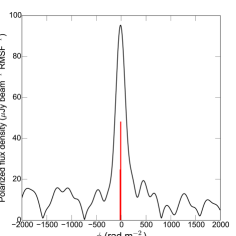
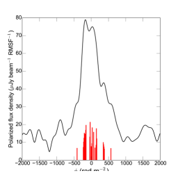
Figure 6: Cleaned Faraday depth spectra (black curves) at different locations in the Antennae uncorrected for the Milky Way contribution. The red lines are the Faraday depth clean components. Left-hand panel: The typical Faraday depth spectra along the tidal tail with a simple profile. The Faraday depth components lies within the step size (10 rad m^-2) of performing the RM synthesis. Middle and right-hand panel: The Faraday depth spectra of two adjacent pixels in the merging disc region which shows complicated Faraday depth spectra with several Faraday depth components.

3.2 Polarized intensity and Faraday depth

The polarized intensity image of the Antennae galaxies at 2.8 GHz determined from the peak of the Faraday depth spectrum is shown in Figure 4. Overlaid segments are the Faraday rotation-corrected magnetic field orientations. Due to our stringent cut of 7$\sigma$ on the peak polarized intensity, we do not detect polarized emission from the entire radio-emitting region. However, we do detect the southern tidal tail, the merging disc and the northern part of NGC 4038. Strongly polarized emission is observed from the tidal tail with median fractional polarization, $\Pi\sim 25$ per cent at 2.8 GHz. The polarized intensity spans a projected linear size of $\sim 20$ kpc, longer than the extent of the detectable total intensity emission. The magnetic field vectors are well aligned along the entire length of the tail. In the region of the merging discs, the polarized emission is weakly polarized (median $\Pi\sim 1.6$ per cent) and the magnetic field is more randomly oriented. The polarized emission and the magnetic field vectors in the northern galaxy NGC 4038 follow a spiral pattern, however, this emission is offset outward (to the west) with respect to the remnant spiral arm. The peak of the polarized emission is shifted outward by $\sim 1.6$ kpc from the peak of the total intensity. Such an offset of the polarized emission was also seen in the 4.85 GHz observations of Chyży & Beck (2004). The polarized emission along the peak of the total radio continuum emission in the remnant spiral arm remains undetected. This region also hosts sites of intense star formation and hence the polarized emission is likely depolarized due to turbulent magnetic fields.

We did not detect any polarized emission at 2.8 GHz from the southern part of the galaxies in general, in particular around the dark cloud complex. At 7$\sigma$ cutoff, this corresponds to a $\Pi\lesssim 0.2$ per cent, comparable to the instrumental leakage. This region shows strong Faraday depolarization between the 4.86 and 8.44 GHz observations of Chyży & Beck (2004). Moreover, they found the percentage polarization to be $\lesssim 1$ per cent at 8.44 GHz. Since, this region also hosts strong thermal emission, the high $n_{e}$ would lead to high Faraday depth. Therefore, the low fractional polarization can be caused by either strong wavelength$-$($\lambda-$)dependent depolarization or by $\lambda-$independent depolarization due to turbulent magnetic fields within the beam.

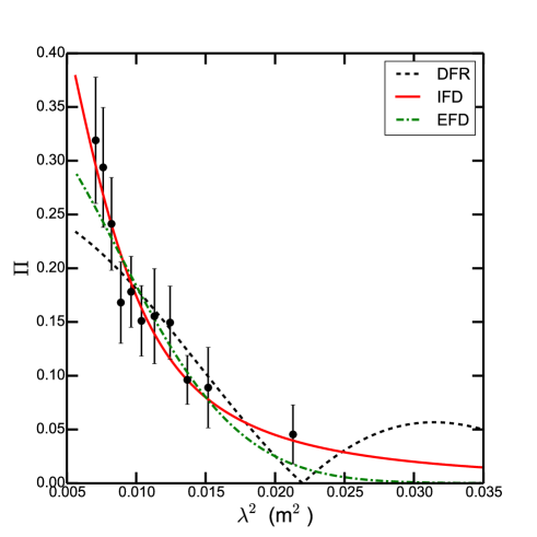
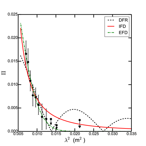
Figure 7: Variation of the fractional polarization ($\Pi$) with $\lambda^{2}$ in the tidal tail (left-hand panel) and the merging region (right-hand panel). The points with arrows are the 2$\sigma$ upper limits. The lines are the fitted models of different types. For the tidal tail, the IFD model provides the best fit and in the merging disc region, EFD model fits the data best.

In left-hand panel of Figure 5, we show the Galactic foreground-corrected map of the Faraday depth of the Antennae and its pixel-wise distribution in the right-hand panel. Faraday depth along the tidal tail vary smoothly having a mean of $+25$ rad m^-2 and a standard deviation of 22 rad m^-2 (shown as the blue histogram) measured over several beams in the plane of the sky. In the northern polarized arm, we find the mean Faraday depth to be $+9.3$ rad m^-2 with dispersion of 20.5 rad m^-2 (shown as the red histogram). The dispersion of Faraday depth around its mean value is larger than that of the tidal tail, suggesting the magnetic field is more ordered in the tidal tail.

The merging disc has strong $\phi$ variations in the range $-100$ to $+140$ rad m^-2. The pixel-wise distribution of $\phi$ in this region shows two peaks (shown as the green histogram in Figure 5) at $\sim-25$ rad m^-2 and $\sim+40$ rad m^-2. The Faraday depth in this region is observed to change sign abruptly and is co-spatial with the systemic velocity of the Hi emission. The Faraday depth spectra in this region have complicated structures having highly dispersed $\phi$ components as compared to other regions. The middle and the right-hand panels of Figure 6 show the Faraday depth spectra at two adjacent pixels where the sign change is observed. Clearly, the spectra are not single peaked as compared to the spectra in the tail (left-hand panel). For the middle panel, the Faraday depth spectrum has a peak at $+68$ rad m^-2, while for the right-hand panel, the Faraday depth spectrum peaks at $-130$ rad m^-2. The restoration of the multiple clean $\phi$ components (shown as red lines in Figure 6) with the RMSF of 219 rad m^-2 gives rise to complicated, broad Faraday depth spectrum. The merging region possibly hosts extended Faraday depth structures, however it is not clear whether the multiple components are indeed different Faraday depth components or one (or multiple) broad components. Therefore, it is not clear if the sign change we observe in Faraday depth is real. Both high angular and Faraday depth resolution are needed along with larger wavelength coverage at lower frequencies to study Faraday depolarization and the nature of the magneto-ionic medium of the merging disc.

3.3 Faraday depolarization

The maximum fractional polarization ($\Pi_{\rm max}$) arising due to synchrotron emission is given by $\Pi_{\rm max}=(1-\alpha_{\rm nt})/(5/3-\alpha_{\rm nt})$ and lies in the range $0.7-0.75$ for $\alpha_{\rm nt}$ in the range $-0.7$ to $-1.1$. However, we seldomly observe this theoretical maximum because the polarized emission can be depolarized due to: (1) $\lambda-$independent beam depolarization caused by random magnetic fields on scales smaller than the beam, (2) bandwidth depolarization caused by Faraday rotation within a finite bandwidth and/or (3) $\lambda-$dependent depolarization depending on the nature of the magneto-ionic medium (see e.g., Sokoloff et al., 1998; O’Sullivan et al., 2012). Studying the nature of the $\lambda-$dependent depolarization can help us to determine the properties of the magneto-ionic medium. However note, the signal-to-noise ratio (SNR) per 8-MHz channel is insufficient to estimate the polarized intensity. Hence, we averaged over each spectral window of 108 MHz width, after flagging the edge channels.

To improve the SNR further, we studied the $\lambda-$dependent depolarization averaged over the tidal tail, the merging disc and the northern region of NGC 4038. To account for beam depolarization while averaging the extended emission over the region of interest, we computed $\Pi$ by averaging the pixels in Stokes $Q$ and $U$ maps as $\Pi=\sqrt{\langle Q\rangle^{2}+\langle U\rangle^{2}}/\langle I_{\rm nt}\rangle$. We find evidence of strong $\lambda-$dependent depolarization in all parts of the Antennae. Due to limited signal-to-noise ratio in individual channel maps, detailed fitting of the Stokes $Q$ and $U$ versus $\lambda^{2}$ as done for the galaxy M 51 by Mao et al. (2015) was not possible. Hence, we fitted the fractional polarization as a function of $\lambda^{2}$ using the simple models given in O’Sullivan et al. (2012) based on Sokoloff et al. (1998).

We note that the depolarization between 2 and 3.6 GHz is $\sim 0.15$. For this depolarization to arise due to bandwidth depolarization because of averaging over 108 MHz, $|\phi|\gtrsim 10^{3}$ rad m^-2 is required. The maximum observed $\phi$ is $\sim 150$ rad m^-2 and thus bandwidth depolarization is not the dominant depolarization mechanism. Therefore, we do not consider this effect in our future calculations.

3.3.1 Tidal tail and merging disc

To assess which mechanism causes the $\lambda-$dependent depolarization, we model the polarization fraction as a function of $\lambda^{2}$ using the different depolarization models given in Sokoloff et al. (1998): differential Faraday rotation (DFR), internal Faraday dispersion (IFD), and external Faraday dispersion (EFD). In Figure 7, we show the variation of the $\Pi$ with $\lambda^{2}$ computed within each spectral window of $\sim 108$ MHz width. The left-hand panel is for the tail region and the right-hand panel is for the merging disc region.

For the tidal tail region, $\Pi(\lambda)$ is best fitted by the IFD model (red solid line in Figure 7 left-hand panel) with $\chi^{2}=3.2$ as compared to $\chi^{2}$ of 10.3 and 5.7 for the DFR and EFD models, respectively. As per the IFD model, the Faraday-rotating medium contains turbulent magnetic fields along the line-of-sight and is also emitting synchrotron radiation. In this case $\Pi(\lambda)$ varies as

$$\Pi(\lambda)=\Pi_{\rm int}\left(\frac{1-e^{-S}}{S}\right).$$ (2)

Here, $\Pi_{\rm int}$ is the $\lambda-$independent intrinsic polarization fraction, and $S=2\sigma_{\rm RM}^{2}\lambda^{4}$, where $\sigma_{\rm RM}$ is the Faraday dispersion within the 3D beam arising from turbulent fields. We find $\sigma_{\rm RM}=131\pm 23$ rad m^-2 and internal polarization fraction of $0.62\pm 0.18$ close to the theoretical value.

Similarly, for the merging disc region, $\Pi(\lambda)$ is best fitted by an external dispersion screen (green dashed-dot line in Figure 7 right-hand panel) with $\chi^{2}=1.5$. The fits with DFR and IFD models gives $\chi^{2}$ of 4.8 and 6.1, respectively. In an external dispersion screen, the Faraday rotating medium, lying between the observer and the synchrotron emitting media, contains random magnetic field along the line of sight. In this case $\Pi(\lambda)$ is given by

$$\Pi(\lambda)=\Pi_{\rm int}e^{-2\sigma_{\rm RM}^{2}\lambda^{4}}.$$ (3)

We find the internal polarization fraction to be $0.040\pm 0.006$ and $\sigma_{\rm RM}=99\pm 5$ rad m^-2.

3.3.2 Star-forming regions

We did not detect any polarized emission from the dark cloud and star-forming regions located in the southern part of NGC 4038/9. While the synchrotron emission is the strongest in these regions, non-detection of polarized emission at the resolution of our observations (corresponding to $\sim 1$ kpc linear scales) suggests the magnetic field could be random at much smaller scales. However, we could estimate the effects of Faraday depolarization in these regions using the estimated thermal emission. The free–free optical depth ($\tau_{\rm ff}$) at a radio frequency ($\nu$) is related to the thermal flux density ($S_{\rm th,\nu}$) as $S_{\rm th,\nu}=2kT_{e}\nu^{2}\Delta\Omega(1-e^{-\tau_{\rm ff}})/{c^{2}}$. Here, $\Delta\Omega$ is the solid angle subtended by the source and $T_{e}$ is the electron temperature assumed to be $10^{4}$ K. The $\tau_{\rm ff}$ is related to the emission measure (EM) as

$$\tau_{\rm ff}=0.082~{}T_{e}^{-1.35}\nu^{-2.1}\textrm{EM}.$$ (4)

Here, $n_{e}$ is the thermal electron density and is related to the EM as $n_{e}\approx(\textrm{EM}~{}f/h_{\rm ion})^{1/2}$, where $f$ is the filling fraction. In a star-forming disc, the EM predominantly arises from the Hii regions with small filling factors, $f\sim 5$ per cent (Ehle & Beck, 1993; Beck, 2007). $h_{\rm ion}$ is the line-of-sight depth of the ionized gas assumed to be the linear size of the star-forming regions and is observed to have similar size as the resolution of our observations ($\sim 1$ kpc) as seen in the H$\alpha$ images. Using the thermal emission, we estimate the typical $n_{e}$ to be $\sim 3-5$ cm^-3. Thus, the $|\phi|$ for a regular magnetic field of $\sim 1$ kpc scale having strength $|B_{\parallel}|\sim 3-5~{}\mu$G (see § 3.4.2) is $\sim 1-2\times 10^{4}~{}\rm rad~{}m^{-2}$.

For $|\phi|\approx 2\times 10^{4}$ rad m^-2, the effect of bandwidth depolarization is severe below 1.5 GHz within a channel width of 8 MHz. This effect is less than 20 per cent at 3 GHz and our observations are sensitive to $|\phi|\sim 10^{4}$ rad m^-2. Thus, our estimated $|\phi|$ of $\sim 1-2\times 10^{4}$ rad m^-2 in the southern part of NGC 4038/9 may not depolarize the emission at the higher frequency end of our observations. Moreover, the fractional polarization in these regions was found to be $\sim 1$ per cent at 8.44 GHz (Chyży & Beck, 2004), where the effect of bandwidth depolarization is even lower. Thus, owing to the extreme environment and turbulence driven by super starclusters, we conclude that the effects of Faraday depolarization could be severe.

3.4 Magnetic field properties

3.4.1 Total magnetic field strength

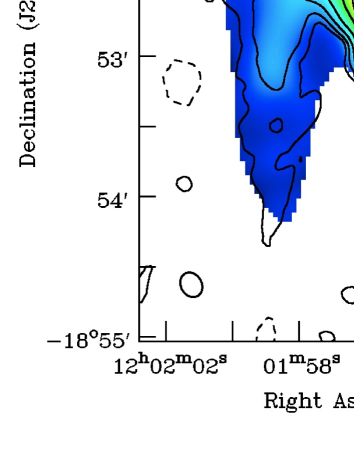
Figure 8: Total magnetic field strength (in $\mu$G) estimated using the non-thermal emission and by assuming energy equipartition between magnetic fields and cosmic ray particles. Overlaid are the total intensity contours same as Figure 1.

The total magnetic field strength ($B_{\rm tot}$) was computed assuming equipartition of energy between magnetic field strength and cosmic ray particles using the revised equipartition formula by Beck & Krause (2005). Figure 8 shows the magnetic field strength map overlaid with the total intensity contours. We used the non-thermal emission at 2.8 GHz and the non-thermal spectral index map to compute the field strength. In addition, we assumed a synchrotron path length $l=2$ kpc, corrected for inclination and the ratio of number densities of relativistic protons to electrons ($K_{0}$) of 100. The average magnetic field strength in NGC 4038/9 is found to be $\sim 20~{}\mu$G, significantly stronger than that of normal star-forming galaxies having typical magnetic field strength of $\sim 10~{}\mu$G (Basu & Roy, 2013; Van Eck et al., 2015). Our estimated magnetic field strength is consistent with that obtained in Chyży & Beck (2004). Note that our assumption of a constant $l$ throughout the Antennae galaxies is likely not realistic and the estimated magnetic field can be scaled by $[2\times 10^{-2}(K_{0}+1)/l_{\rm kpc}]^{1/(\alpha_{\rm nt}+3)}$ due to the assumption of $K_{0}=100$ and $l=2$ kpc. A factor of 2 difference in the path length in different parts of the galaxies would change the field strength estimate by less than 20 per cent.

Within the merging disc, the magnetic field is strong: from $\sim 10~{}\mu$G in the periphery to $\sim 25~{}\mu$G. The magnetic field strength is strongest, $\sim 35~{}\mu$G, in the dark dusty cloud complex. This strong magnetic field is likely produced by the fluctuation dynamo (Subramanian, 1998) driven by high star formation activity. We detect low surface brightness synchrotron emission from the tidal tail with an equipartition field strength of $\sim 6-10~{}\mu$G. However, because of significant energy loss of the CREs in the tidal tail (see §3.1.1), the energy spectral index between CREs and cosmic ray proton differs. The energy spectral indices for cosmic ray protons and electrons are assumed to be constant and the same in the revised equipartition formula. We have therefore set $\alpha_{\rm nt}$ as $-1$ in the tidal tail region and thus the field strength are underestimated.

3.4.2 Ordered magnetic field strength

Table 1: The equipartition magnetic field strengths (in $\mu$G) of the different magnetic field components at various region of the Antennae galaxies. $B_{\rm tot}$ is the total strength, $B_{\rm turb}$ is the strength of the turbulent field, $B_{\rm ord,\perp}$ is the ordered component in the plane of the sky and $B_{\rm ord,\parallel}$ is the ordered component along the line of sight. We have assumed a 3D isotropic turbulent field.

Region	$B_{\rm tot}$	$\frac{B_{\rm turb}}{B_{\rm ord,\perp}}$	$\frac{B_{\rm turb}}{B_{\rm ord,\parallel}}$	$B_{\rm turb}$	$B_{\rm ord,\perp}$	$B_{\rm ord,\parallel}$
	($\mu$G)			($\mu$G)	($\mu$G)	($\mu$G)
(1)	(2)	(3)	(4)	(5)	(6)	(7)
Southern tail	10	0.6	5.8–9.2	5	8.5	$<1$
Merging disc	20	7–12	4–5	19.5	$<5$	$<5$
Northern arm	20	$<3.7$	–	19	$<6$	–
Star-forming	25–35	–	–	–	–	–

The internal degree of polarization ($\Pi_{\rm int}$) is related to the ratio of the 3D isotropic turbulent field ($B_{\rm turb}$) and the ordered magnetic field in the plane of the sky ($B_{\rm ord,\perp}$). Under the assumption of equipartition, $\Pi_{\rm int}$ is related to $q=B_{\rm turb}/B_{\rm ord,\perp}$ by (Sokoloff et al., 1998)

$$\Pi_{\rm int}=\Pi_{\rm max}\frac{\left(1+\frac{7}{3}q^{2}\right)}{\left(1+3q^{2}+\frac{10}{9}q^{4}\right)}.$$ (5)

We note that, the above relation assumes the ordered magnetic fields lies entirely in the plane of the disc. Thus, for a realistic scenario of a non-zero ordered magnetic field component perpendicular to the disc, especially for the merging galaxies, $B_{\rm ord,\perp}$ would be overestimated. Furthermore, since, $B_{\rm tot}^{2}=B_{\rm ord}^{2}+B_{\rm turb}^{2}=B_{\rm turb}^{2}\left[1+q^{-2}+(B_{\rm ord,\parallel}/B_{\rm turb})^{2}\right]$, the above assumption does not affect the estimation of $B_{\rm turb}$ using $q$ if the turbulent field is isotropic, but it affects the regular field strength estimation. This is because what we actually measure is $1/q_{\rm obs}^{2}=1/q^{2}+(B_{\rm ord,\parallel}/B_{\rm turb})^{2}$.

At the frequency of our observations, the fractional polarization is strongly affected by $\lambda-$dependent depolarization, therefore we are unable to produce a map of $B_{\rm ord,\perp}$. We use the fitted values for $\Pi_{\rm int}$ from §3.3.1 to estimate $B_{\rm ord,\perp}$. We further use the ratio $\sigma_{\rm RM}/\langle{\rm RM}\rangle$ to estimate $B_{\rm ord,\parallel}/B_{\rm turb}$ (see §4.1). In the tidal tail, the average $B_{\rm tot}$ is $\sim 10~{}\mu$G, $B_{\rm turb}$ is $\sim 5~{}\mu$G and the $B_{\rm\perp,ord}$ is $\sim 8.5~{}\mu$G. In the merging disc, the total field strength is found to be $\sim 20~{}\mu$G. This gives a turbulent field strength of $19.5~{}\mu$G for the fitted $\Pi_{\rm int}$ of $\sim 0.04$ and the upper limit on the $B_{\rm ord,\perp}$ of $2.7~{}\mu$G. The magnetic field strength estimates in different regions of the Antennae are summarized in Table 1.

4 Discussion

4.1 Regular field of $\sim 20$ kpc in the tidal tail

We detect highly polarized emission along the southern tidal tail of the Antennae with intrinsic polarization fraction close to the theoretical maximum (see §3.3.1). The magnetic field orientations in the plane of the sky corrected for Faraday rotation are well-aligned along the tail (see Figure 4). Such a high degree of polarization can originate from a combination of anisotropic turbulent magnetic fields by compressing an initially random field, and regular magnetic fields in the plane of the sky (Beck, 2016). However, anisotropic fields dominating over the regular field will not contribute to Faraday depth (Jaffe et al., 2010). From our data, we find the Milky Way foreground-corrected Faraday depth along the tidal tail varies smoothly with positive sign throughout (see Figure 5) indicating the line-of-sight ordered field points toward the observer. Anisotropic random fields alone cannot give rise to a smooth large-scale variation of Faraday depth measured over several beams. We therefore conclude that the magnetic field in the plane of the sky along the tidal tail is regular (or coherent) and maintains its direction over $\sim 20$ kpc. To our knowledge, this is the largest coherent magnetic field structure observed in galaxies. We discuss in detail the properties of the magneto-ionic medium in the tidal tail.

4.1.1 Turbulent cell size

The standard deviation of the Faraday depth within the 3D beam ($\sigma_{\rm RM}$) in the tidal tail region is found to be $131$ rad m^-2 (see §3.3.1). This dispersion of the RM is caused by fluctuations of the field strength along the line of sight. The $\sigma_{\rm RM}$ depends on the turbulent magnetic field along the line of sight and the properties of the magneto-ionic medium as

$$\sigma_{\rm RM}=0.81\left(\frac{\langle n_{\rm e}\rangle}{\rm cm^{-3}}\right)\left(\frac{B_{\rm turb,\parallel}}{\rm\mu G}\right)\left(\frac{L_{\rm ion}d}{f}\right)^{1/2}.$$ (6)

Here, $\langle n_{\rm e}\rangle$ is the average thermal electron density along the line of sight, $B_{\rm turb,\parallel}$ is the strength of the random magnetic field along the line of sight, $L_{\rm ion}$ is the path length through the ionized medium (in pc), $d$ is the size of the turbulent cells (in pc) and $f$ is the volume filling factor of electrons along the line of sight. The RM dispersion in the plane of the sky ($\sigma_{\rm RM,sky}$) is related to the $\sigma_{\rm RM}$ as (Fletcher et al., 2011)

$$\sigma_{\rm RM,sky}\simeq N^{-1/2}\sigma_{\rm RM},$$ (7)

where, $N\approx(D/d)^{2}$ is the number of turbulent cells for the projected beam area in the sky of diameter $D$, for which $\sigma_{\rm RM,sky}$ is measured. Thus, we can compute the diameter of typical turbulent cell size $d$ using the observed $\sigma_{\rm RM,sky}$, $\sigma_{\rm RM}$, and the beam size $D\approx 1400$ pc. $d$ is found to be $\sim 230$ pc, significantly larger than the typical turbulent cell size of $\sim 50$ pc observed in the discs of galaxies (Fletcher et al., 2011; Mao et al., 2015; Haverkorn et al., 2008). Hence, assuming the line of sight extent of the tidal tail to be the same as the thickness in the plane of sky, i.e. $L_{\rm ion}=1.1$ kpc, the field along the line of sight must be regular. Therefore, the observed dispersion of the Faraday depth must be caused by systematic variations in the plane of the sky. The Faraday depth indeed varies smoothly in the tidal tail (see Figure 5).

4.1.2 Regular field strengths

The mean RM depends on the regular component of the magnetic field along the line of sight ($B_{\rm reg,\parallel}$) as

$$\langle{\rm RM}\rangle=0.81\langle n_{\rm e}\rangle B_{\rm reg,\parallel}L_{\rm ion}.$$ (8)

Thus, the ratio of $\sigma_{\rm RM}$ to $\langle\rm RM\rangle$ can give us the estimate of $B_{\rm turb,\parallel}/B_{\rm reg,\parallel}$ and is given by

$$\frac{\sigma_{\rm RM}}{|\langle\rm RM\rangle|}=\frac{B_{\rm turb,\parallel}}{|B_{\rm reg,\parallel}|}\left(\frac{d}{fL_{\rm ion}}\right)^{1/2}.$$ (9)

From our estimated values of $\sigma_{\rm RM}$, $\langle\rm RM\rangle$ and $d$, and assumed value for $L_{\rm ion}$, we find $B_{\rm turb,\parallel}/B_{\rm reg,\parallel}\sim 13f^{1/2}$. Compared to the star-forming disc, the ionized medium in the tidal tail is more diffuse. Therefore, assuming typical $f$ in the range $0.2-0.5$ for a diffuse medium, $B_{\rm turb,\parallel}/B_{\rm reg,\parallel}$ lies in the range $5.8-9.2$. Assuming $B_{\rm turb}=5~{}\mu$G is isotropic (see §3.4.2), we estimate $B_{\rm reg,\parallel}$ to be $\lesssim 1~{}\mu$G. Thus, the field strength in the plane of the sky ($B_{\rm reg,\perp}\sim 8.5~{}\mu$G) is significantly larger than $B_{\rm reg,\parallel}$, perhaps caused due to stretching and twisting of the remnant spiral field in the disc of the galaxies during the tidal interaction.

Here, we explore the degree of stretching required to amplify an initial regular field in the progenitor galaxy to the observed field strengths in the tidal tail. For this, we consider the scenario that an initially cylindrical spiral-shaped regular field generated in the progenitor galaxies by dynamo action has been stretched by the tidal interaction. Assuming the field is stretched keeping the cross-sectional area constant, then the ratio $B/\rho l$ is conserved if the magnetic flux is frozen in the tube (see e.g., Longair, 2011). Here, $\rho$ is the density of the gas and $l$ is the length of the cylinder. From observations of Hi gas (Hibbard et al., 2001), the density in the tidal tail is about a factor of 3 lower than that in the remnant spiral arm. Therefore, a regular field of 8.5 $\mu$G in the tidal tail requires stretching by a factor of $\sim 4-9$ for an initial regular field of $\sim 3-6~{}\mu$G in strength (see §4.3). This implies, the dynamo generated initial field was regular over $\sim 2-5$ kpc, which is a typical length-scale observed in nearby spiral galaxies (Beck & Wielebinski, 2013). Thus, tidal stretching of field lines can also amplify large-scale regular fields within the dynamical time-scale of the merger event, i.e., few 100 Myr. A full treatment of the 3D magnetic field structure is beyond the scope of this paper and will be discussed in a forthcoming paper (A. Basu et al. 2016 in preparation).

4.1.3 Thermal electron densities

Using Equation 8, and the upper limit on $B_{\rm\parallel,reg}$, we constrain $\langle n_{\rm e}\rangle$ to be $\gtrsim 0.02$ cm^-3 in the tidal tail. The column density of the Hi in the tidal tail is found to be $\sim 6\times 10^{20}$ cm^-2 having thickness $\sim 4.5$ kpc (Hibbard et al., 2001) which corresponds to $\langle n_{\rm H}\rangle\sim 0.04$ cm^-3. Thus, from our constraint on the $\langle n_{\rm e}\rangle$, the ionization fraction in the tidal tail is $\gtrsim 30$ per cent. As pointed out in the study by Hibbard et al. (2005), the UV emission from the tidal tail predominantly arises from old stars, and there is little evidence of on-going star formation. This is insufficient to sustain the ionic medium and therefore the ionization of the tidal tail is maintained by the inter-galactic radiation field.

4.2 Turbulent fields in the merging disc

The polarized emission from the merging disc of the galaxies has low fractional polarization with a median value of only $\sim 0.016$ at 2.8 GHz and the $\lambda-$dependent depolarization is best described by an external dispersion screen (see §3.3). From the fitted value of $\sigma_{\rm RM}\approx 100$ rad m^-2 and observed $|\langle\rm RM\rangle|\approx 40$ rad m^-2, we find $B_{\rm turb,\parallel}/B_{\rm ord,\parallel}\approx 16f^{1/2}$, assuming path length $L_{\rm ion}=2$ kpc and a typical turbulent cell size of $\sim 50$ pc observed in discs of galaxies. Hence, $B_{\rm turb,\parallel}/B_{\rm ord,\parallel}$ ranges from 4–5 for $f$ in the range 0.05–0.1. The measured low $\Pi_{\rm int}$ of 0.04 is likely caused by a turbulent magnetic field enhanced due to the merger event. For the estimated $\Pi_{\rm int}$ of 0.04, we find $B_{\rm turb,\perp}/B_{\rm ord,\perp}$ in the range 7–12, i.e., the turbulent field strength significantly dominates over the ordered field both in the plane of the sky and along the line of sight. For isotropic turbulence, $B_{\rm turb}$ is found to be $\sim 19.5~{}\mu$G. Using this, we constrain the strength of the regular fields along the line of sight $B_{\rm ord,\perp}$ to be $\lesssim 5~{}\mu$G, and in the plane of the sky, $B_{\rm ord,\parallel}\approx 1.2f^{-1/2}\lesssim 5~{}\mu$G for $f\gtrsim 0.05$.

4.3 Ordered fields in the northern arm

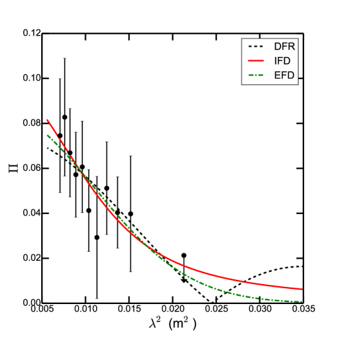
Figure 9: Variation of the fractional polarization ($\Pi$) with $\lambda^{2}$ around the northern spiral arm region. The point with arrow is the 2$\sigma$ upper limit. The lines are the best fit models of different types.

The polarized emission from the relic spiral arm of NGC 4038 in the north is weak with median $\Pi\sim 0.08$ at 2.8 GHz. The $B_{\rm\perp,reg}$ is observed to follow a spiral pattern (see Figure 3). The polarized emission is depolarized in the optical spiral arm hosting sites of high star formation and the detected polarized emission is offset toward the outer parts. It is difficult to reliably measure the fractional polarization as the total intensity quickly falls off to the background noise level in that region. The mean Faraday depth of this feature is $\sim+9$ rad m^-2 and has a comparatively large dispersion of $\sim 20$ rad m^-2 in the plane of the sky varying between $-30$ to $+40$ rad m^-2 (see Figure 5). We observe the Faraday depth to frequently change sign smoothly over a few synthesized beam, indicative of a less coherent regular component of the magnetic field in the plane of the sky than that in the tidal tail.

In Figure 9, we show the variation of $\Pi$ as a function of $\lambda^{2}$ in the northern arm region. Due to a limited $\lambda^{2}$ coverage of our data, it is not possible to select a best fit model from our data ($\chi^{2}=2.2,1.6$ and $1.8$ for the DFR, IFD and EFD models, respectively). All the depolarization mechanisms indicate a $\Pi_{\rm int}$ between 0.08–0.1 and if we assume isotropic turbulent fields, $B_{\rm turb}$ is estimated to be $\sim 19~{}\mu$G. Since, we do not have a estimate of $B_{\rm turb,\parallel}/B_{\rm ord,\parallel}$ due to lack of unambiguous fit to Faraday depolarization, we estimate an upper limit on the strength of $B_{\rm ord,\perp}$ as $6~{}\mu$G.

4.4 Extreme Faraday depolarization in southern star-forming regions

The southern part of the Antennae system around the dark cloud region shows strong depolarization, such that the polarized emission remains undetectable in our observations below $\sim 3.6$ GHz, at 4.8 GHz (Chyży & Beck, 2004) and the fractional polarization at 8.44 GHz is extremely low ($\sim 1$ per cent; Chyży & Beck, 2004). Although, such an effect could be caused by $\lambda-$independent beam depolarization due to the random component of the magnetic field, here we assess the possibility of extreme nature of Faraday depolarization.

In §3.3.2 we showed, based on the estimated thermal emission, we expect $|\phi|$ $\sim 10^{4}$ rad m^-2. Such high $\phi$ values are unlikely to cause bandwidth depolarization especially above $\sim 3$ GHz within a 8 MHz channel. Assuming that the $\lambda-$dependent depolarization arises due to the same region being Faraday rotating and synchrotron emitting but with a regular magnetic field along the line of sight, i.e., depolarization due to differential Faraday rotation (DFR), the $\Pi(\lambda)$ is given by

$$\Pi(\lambda)=\Pi_{\rm int}\frac{\sin|\phi\lambda^{2}|}{|\phi\lambda^{2}|}.$$ (10)

In this case, $\phi$ is related to the RM as $\phi=(1/2)\textrm{RM}$. Using this we find, for the estimated $\phi\sim 10^{4}$ rad m^-2, the expected fractional polarization at 8.44 GHz with a bandwidth of 50 MHz (same as the observations of Chyży & Beck, 2004) lies between $1-7$ per cent with occasional null values depending on the $|\phi|$. The variation of the fractional polarization at 8.44 GHz along this region was observed to be spatially smooth (1–2 per cent) and hence it is unlikely that an ionic medium with only a uniform magnetic field gives rise to such high depolarization.

If the magneto-ionic medium is turbulent, driven by high star-formation activity and merger, then the internal and external Faraday dispersion models, give $\sigma_{\rm RM}\sim 10^{3}$ rad m^-2. Using Equation 6 we infer the turbulent cells to be 10–50 pc in size for a turbulent field strength of $\sim 20~{}\mu$G and the estimated $\langle n_{\rm e}\rangle\approx 3~{}\rm cm^{-3}$. The cell size is typical of what is observed in the spiral arms of normal star-forming galaxies (Fletcher et al., 2011; Mao et al., 2015). Hence, it is difficult to disentangle whether the star-forming regions in the southern part are beam depolarized due to a turbulent magnetic field or Faraday depolarized due to extreme properties of the magneto-ionic media. To distinguish between these broadband properties require Stokes $Q$ and $U$ fitting of higher resolution (A- and B-array) and higher frequency (4–8 GHz) data. We have acquired data between 4 and 8 GHz using the VLA in the DnC, CnB and BnA array configurations and the data will be analyzed.

4.5 Implications on the buildup of galactic magnetic fields

Implications on ISM of galaxies: As a late stage merger, the Antennae is a classic example of a system at the peak of the cosmic star formation history. We, however, note that the early merging galaxies are believed to be different in their interstellar medium ISM properties as compared to the present day mergers. The present day merging systems, such as the Antennae galaxies, are predominantly between well-settled, dynamically cold discs with comparatively lower star formation rates as compared to early mergers which can be between more gas-rich, turbulent, and compact systems (Förster Schreiber et al., 2009; Williams et al., 2011; Stott et al., 2016). Based on the bolometric far infrared luminosity, the Antennae pair is classified as a luminous infrared galaxy (LIRG). LIRGs contribute significantly to the comoving star formation density beyond redshift of 1 (Magnelli et al., 2009). Therefore, a detail understanding of the Antennae is essential to understand cosmic evolution of ISM in galaxies. Merger induced active star formation and turbulence (Veilleux et al., 2002) is an essential ingredient in the evolution of hot interstellar gas through stellar feedback (Metz et al., 2004). It is crucial in the rapid amplification of magnetic fields via turbulent-dynamo mechanisms. Our study demonstrates the magnetic field strength in the Antennae is comparatively higher than that in isolated galaxies and is dominated significantly by turbulent fields within the merging bodies.

The turbulent magnetic field—and its coupling with the ISM energy densities, especially the kinetic energy of the turbulent gas—is important in the origin and maintenance of the radio–far infrared correlation at higher redshifts (Schleicher & Beck, 2013). The stronger field strength in merging galaxies ($\sim 20~{}\mu$G) compensate for the inverse-Compton losses due to the cosmic microwave background at higher redshifts and helps in maintaining the radio–far infrared correlation (Basu et al., 2015).

Comparison to the pan-Magellanic field: In the immediate neighbourhood of the Milky Way, the Magellanic bridge connecting the Large and Small Magellanic clouds (LMC and SMC, respectively) could potentially be an example of a system hosting regular magnetic fields of similar length-scale as detected in the tidal tail of Antennae galaxies. Through studies of starlight polarization and RMs inferred from background sources, it has been suggested that an aligned “pan-Magellanic” magnetic field possibly exists, connecting LMC and SMC (Mao et al., 2008; Wayte, 1990). Deinzer & Schmidt (1973) presented model of the Hi gas connecting the two clouds that spans $\sim 20$ kpc, which supports the existence of pan-Magellanic magnetic field. Although, similar to the tidal tail of the Antennae galaxies, the Magellanic bridge is likely generated from a tidal event (Besla et al., 2012; Bagheri et al., 2013), its progenitors are very different from those of the Antennae galaxies both in terms of morphologies and their initial field strengths. Detailed studies of magnetic field properties in LMC and SMC have revealed low total field strengths of $\sim 3~{}\mu$G (Mao et al., 2008, 2012). Therefore, low progenitor magnetic field strengths along with significantly less tidal pressure because of shallow gravitational potential of the LMC–SMC system as compared to that of the Antennae galaxies, the strength of the pan-Magellanic ordered field could be low. For example, the model by Deinzer & Schmidt (1973), predicts the strength of the pan-Magellanic ordered field to be sub-microgauss to a few microgauss.

The pan-Magellanic ordered field could span about 20 degrees on the sky. Therefore, direct detection of the regular field from linearly polarized emission is difficult because of low surface brightness and systematic contribution from the Milky Way in the foreground. To firmly establish the existence of such a field, improved RM grid experiment with a large number of background polarized sources is essential as suggested by Mao et al. (2008). A systematic comparison of the pan-Magellanic magnetic field with that of the tidal tail of the Antennae galaxies is not possible until we have firm observations about the strength and the structure of this pan-Magellanic magnetic field.

Implications on magnetic field measurements at high redshifts: Usually, one studies magnetic field properties in high redshift intervening objects by measuring the excess RM towards quasar absorption line systems: Mgii, damped Lyman-$\alpha$ (DLA), sub-DLA (see e.g., Oren & Wolfe, 1995; Bernet et al., 2008; Joshi & Chand, 2013; Farnes et al., 2014). It has been suggested that the sub-DLAs can originate from neutral gas that lies $\gtrsim 20$ kpc from the host galaxies and the absorbing gas is likely stripped via tidal interaction and/or ram pressure (Sembach et al., 2001; Muzahid et al., 2016). The tidal tail of the Antennae with $N_{\rm HI}$ in the range $\sim 10^{20}-6\times 10^{20}$ cm^-2, would be a classic example of a DLA or sub-DLA (depending on at what distance the from the host galaxies the line-of-sight intersects), when observed as a Lyman-$\alpha$ absorber against a quasar at high redshifts. Our study shows that such systems can host large scale regular magnetic fields and gives rise to rotation measure when observed at suitable viewing angles. It is therefore important to take into account that the inferred field could come from tidally stripped gas, and not only from the disc.

Implications to magnetization of the intergalactic medium: Coherent magnetic fields in the outskirts of merging galaxies, extending in to the intergalactic medium, assists in propagation of cosmic ray particles along the field lines (see e.g., Cesarsky, 1980; Ptuskin, 2006). Thus, apart from starburst driven galactic winds, galaxy mergers can also play an important role in magnetizing the intergalactic medium and enriching it with cosmic ray particles.

Implication to evolution of large-scale fields in galaxies: In a study of cosmological evolution of large- and small-scale magnetic fields in galaxies, Arshakian et al. (2009) predicted that major merger events dissipate the $10^{-6}$ G large-scale disc fields down to several $10^{-8}$ G. Our study comprehensively shows that, although the pre-merger regular magnetic fields in the galactic discs are mostly disrupted by the merger and are dominated by turbulent fields, they can assist in producing larger-scale coherent fields several microgauss in strength through field stretching. The detection of a $\sim 20$ kpc coherent magnetic field in the tidal tail indicates that large-scale fields can be preserved even in advanced merging systems. Moreover, large-scale fields do not necessarily require Gyr timescales to develop as predicted by magneto-hydrodynamic (MHD) simulations (Arshakian et al., 2009; Hanasz et al., 2009). A detailed MHD simulation is essential to understand the nature of the coherent magnetic fields in the tidal tails and its implications in developing large-scale regular fields observed in isolated galaxies in the local Universe.

5 Summary

We have studied the magnetic field properties of the spiral galaxies NGC 4038/9, also known as the Antennae galaxies, undergoing late stage merger. The galaxies were observed between 2 and 4 GHz using the VLA in DnC and CnB arrays and studied the polarization properties using the combined DnC+CnB array data. We summarize our main findings in this section.

1. We estimated the thermal emission from the galaxies using FUV emission as a tracer. We find the mean $f_{\rm th}$ to be $\sim 25$ per cent, significantly higher than what is found in normal star-forming galaxies. The galaxy-integrated $\alpha_{\rm nt}$ is found to be $-1.11\pm 0.03$. The $\alpha_{\rm nt}$ value can have systematic error up to $\sim 10$ per cent due to uncertainties in the thermal emission.

2. We detect the total intensity radio continuum emission from the gas-rich southern tidal tail extending up to $\sim 18$ kpc at $3\sigma$ level. This region shows steep non-thermal spectrum with $\alpha_{\rm nt}$ lying in the range $-1.2$ to $-1.6$, indicating that the tail is composed of an older population of CREs.

3. Employing the technique of RM synthesis, we detect polarized emission from the southern tidal tail extending up to $\sim 20$ kpc. The Faraday depth along the tidal tail varies smoothly preserving its sign throughout. The $\lambda-$dependent Faraday depolarization of this region is best described by an internal Faraday dispersion model with $\sigma_{\rm RM}=131\pm 23$ rad m^-2 and an internal fractional polarization of $0.62\pm 0.18$.

4. Our result suggests that the magnetic field along the tidal tail is highly regular up to a size of $\sim 20$ kpc, the largest known coherent field structure on galactic scales. In this region, the regular field lies mostly in the plane of the sky with $B_{\rm reg,\perp}\approx 8.5\mu$G and dominates over the turbulent field ($B_{\rm turb}\approx 5~{}\mu$G). The large-scale field is likely generated by stretching of an initial disc field by a factor of 4–9 over the merger’s dynamical time-scale of few 100 Myr.

5. We estimate the ionization fraction in the tidal tail to be $\gtrsim 30$ per cent, although there is no indication for on-going star formation that could maintain the ionized medium. Inter-galactic radiation field is likely the main contributor of ionizing photons.

6. The remnant spiral arm in the northern galaxy NGC 4038 has spiral-shaped regular magnetic field structures and it is displaced outward by $\sim 1.6$ kpc with respect to that of the optical and total intensity radio-continuum emission. Here, the Faraday depth varies between $-30$ and $+40$ rad m^-2 and frequently reverses sign along the arm, indicating the magnetic field is less ordered than that in the tail. The magnetic field strength in this region is dominated by the turbulent field ($\sim 19~{}\mu$G).

7. In the merging disc, the $\lambda-$dependent Faraday depolarization is best described by an external Faraday dispersion screen with strong turbulent fields of strength $\sim 19.5~{}\mu$G. Faraday depth spectra in this region have complex structures with multiple and/or broad Faraday depth components. The ordered component of magnetic fields, $B_{\rm ord,\perp}$ and $B_{\rm ord,\parallel}$ is estimated to be $<2.7$ and $<4~{}\mu$G, respectively.

8. The magnetic field strength is strongest in the star-forming regions reaching values up to $\sim 35~{}\mu$G. The polarized emission from the star-forming regions remain undetected at the sensitivity of our observations. This is perhaps caused due to turbulence driven by merger induced intense star formation.

Appendix A Thermal emission separation

The radio continuum emission is mainly a combination of non-thermal synchrotron and thermal free–free emission. Although, the overall contribution of thermal emission to the total radio emission at 1.4 GHz is $\sim 10$ per cent for normal star-forming galaxies (Niklas et al., 1997; Tabatabaei et al., 2007; Basu et al., 2012), the thermal fraction ($f_{\rm th}$) could be much higher—more than 30 per cent in star-forming regions. Detailed studies of the star formation history in the Antennae have revealed intense starbursts in localized regions, especially in the overlapping region and the western galaxy NGC 4038 (Zhang et al., 2010; Klaas et al., 2010). Such regions are bright in H$\alpha$, coincident with the peaks in the total radio continuum emission (see Figure 1) due to enhanced thermal emission. We estimated the thermal emission on a pixel-by-pixel basis using star formation rate (SFR) as its tracer following Condon (1992). The thermal emission ($S_{\rm\nu,th}$) at a radio frequency $\nu$ is related to SFR as

$$\left(\frac{S_{\rm\nu,th}}{\rm Jy}\right)\approx 4.6D_{\rm Mpc}^{-2}\nu_{\rm GHz}^{-0.1}\left(\frac{\textrm{SFR}}{\rm M_{\odot}yr^{-1}}\right).$$ (11)

Here, $D_{\rm Mpc}$ is the distance to the galaxy in Mpc. We used the GALEX far-ultraviolet (FUV; $\lambda\approx 1520\AA$) image to estimate SFR using the calibration given in Kennicutt & Evans (2012). We corrected the FUV emission for dust extinction using the observed FUV–NUV colour ($(FUV-NUV)_{\rm obs}$; Hao et al. 2011)

$$A_{\rm FUV}=(3.83\pm 0.48)\times[(FUV-NUV)_{\rm obs}-(0.022\pm 0.024)].$$ (12)

The large error in the attenuation ($A_{\rm FUV}$) calibration gives rise to up to $\sim 20$ per cent error in extinction correction for the range of $(FUV-NUV)_{\rm obs}$ in the Antennae galaxies. The highest extinction is observed around the central regions of the two galaxies and along the spiral arms. In those regions, the estimated SFR, and hence the thermal emission, can be uncertain by at most 30 per cent. We estimate the total SFR for the Antennae galaxies to be $\sim 10~{}\rm M_{\odot}~{}yr^{-1}$ which is in agreement with total SFR of $13~{}\rm M_{\odot}~{}yr^{-1}$ estimated by Klaas et al. (2010) using total infrared emission within 30 per cent.

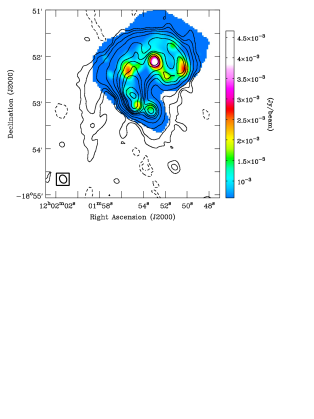
Figure 10: Thermal emission map of the Antennae galaxies estimated using extinction corrected FUV emission. The overlaid total intensity contours are same as Figure 1.

Our estimated total SFR of 10 $\rm M_{\odot}~{}yr^{-1}$ corresponds to a total thermal emission of $86$ mJy, hence mean $f_{\rm th}\sim 25$ per cent at 2.8 GHz. In Figure 10, we show the thermal emission map of the Antennae galaxies. The estimated $f_{\rm th}$ is in good agreement with 27 per cent at 2.8 GHz estimated by interpolating $f_{\rm th}\approx 50$ per cent at 10.45 GHz for the flux density scale assumed in Chyży & Beck (2004). The mean $f_{\rm th}$ is significantly higher than what have been observed for normal star-forming galaxies. The western galaxy NGC 4038 have comparatively higher $f_{\rm th}$ of $\sim 30$ per cent at the centre and $\sim 24$ per cent in its remnant spiral arm. These regions host intense star formation likely induced by the merger (Zhang et al., 2010). In the dark cloud region, radio emission is significantly dominated by non-thermal emission where $f_{\rm th}\lesssim 8$ per cent. This is also the region where $f_{\rm th}$ is lowest.

We note that our thermal emission could be overestimated because of FUV emission was used as a tracer of star formation. The thermal emission is best traced by H$\alpha$ emission originating from ionization by young ($\lesssim 10$ Myr) and massive ($\gtrsim 10~{}\rm M_{\odot}$) stars. While, the FUV emission could also originate from an older population (10–100 Myr) of lower mass stars (Kennicutt & Evans, 2012). The contribution of the older stellar population to the FUV emission therefore overestimates the recent SFR and the thermal emission can be overestimated. We could not use the H$\alpha$ emission for estimating the thermal emission because the only publicly-available continuum subtracted H$\alpha$ map does not cover the entire Antennae galaxies (see e.g., Whitmore et al., 1999).

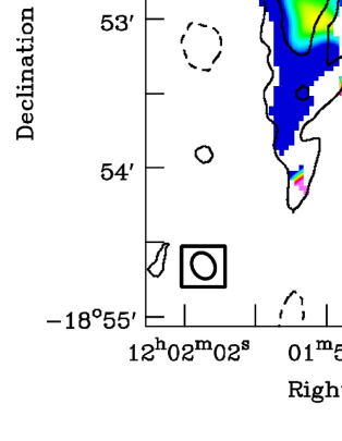
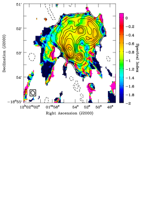
Figure 11: Left-hand panel: In-band spectral index map between 2 and 3.6 GHz at an angular resolution $15\times 12$ arcsec² produced by power-law fitting of total intensity images of each spectral window on a pixel-by-pixel basis. Right-hand panel: Spectral index map produced using the clean task in casa with nterms=2 at an angular resolution $11\times 9$ arcsec². The overlaid total intensity contours are same as Figure 1. Note that, at low signal-to-noise ratio regions, especially in the outer parts, the spectral index computed by casa gives rise to unphysically flat or inverted spectrum, unlike in the left-hand panel.

Appendix B Spectral index distribution

The total intensity maps of each spectral window were used to compute the in-band spectral index ($\alpha$) between 2 and 3.6 GHz of the Antennae galaxies. The spectral index map for NGC 4038/9 was computed by fitting a power law of the form, $\log S_{\nu}=\beta+\alpha\log\nu$, to each pixel of the total intensity maps across the 11 spectral window images. Here, $S_{\nu}$ is the total flux density at a frequency $\nu$ and $\beta$ is the normalization constant at $\nu=1$ GHz. We convolved the total intensity images of all the 11 spectral windows to a common resolution of $15\times 12$ arcsec² (the resolution at the lowest frequency). All the maps were then aligned to a common coordinate system to do the fitting. The left-hand panel of Figure 11 shows the spectral index map. The galaxy-integrated spectral index between 2–3.6 GHz, estimated by fitting the integrated total intensities shown in Figure 2, is found to be $-0.85\pm 0.02$. The spectral index shows large variations between $-0.6$ in the dark cloud complex and $<-1.2$ in the tidal tail. The typical error on the fitted values of spectral index in high signal-to-noise ratio (SNR; $\gtrsim 10$) pixels is $\lesssim 5$ per cent. In low SNR ($\lesssim 5$) pixels, especially in the outer parts and tidal tail, the spectral index error is up to $\sim 25$ per cent. The variation of the spectral index is in good agreement with Chyży & Beck (2004).

The task clean with nterms=2 in casa can also produce a spectral index map through modelling the sky brightness as a Taylor-series expansion per frequency channel (see Rau & Cornwell, 2011). In right-hand panel of Figure 11 we show the spectral index map computed using casa. Note that, the colour-scale of the two maps are different in order to represent the full range of values. In regions with high SNR ($\gtrsim 6$) in inner parts of the Antennae, both the methods are in excellent agreement with each other. But, in regions with $\textrm{SNR}\lesssim 5$, especially in the outer parts of the extended emission, the spectrum computed by casa is either flat or inverted which is unrealistic. Our fitting does not produce $\alpha$ with values $\gtrsim-0.3$.

The differences in $\alpha$ in the outer parts is not critical for our analysis, but we prefer to use the pixel-by-pixel fitting method as it enables us to compute the non-thermal spectral index map. The non-thermal spectral index, $\alpha_{\rm nt}$, was computed after subtracting the thermal emission map scaled to the frequencies of each spectral window. A similar pixel-by-pixel fitting was done using the non-thermal emission map of each spectral window. The green dash-dot line in Figure 2 represents the thermal emission with a spectral index of $-0.1$. The non-thermal emission at each spectral window after subtracting the thermal emission from the total intensity are shown as the red squares. The galaxy-integrated $\alpha_{\rm nt}$ estimated by fitting the total non-thermal emission at each spectral window is found to be $-1.11\pm 0.03$ and is shown as the red dashed line in Figure 2. However, the estimated $\alpha_{\rm nt}$, overall, can have systematic error up to $\sim 10$ per cent due to uncertainty in the estimated thermal emission. In spatially resolved case, the uncertainty in the thermal emission affects $\alpha_{\rm nt}$ up to 10 per cent in bright regions where $f_{\rm th}$ is high. The errors in $f_{\rm th}$ do not affect $\alpha_{\rm nt}$ in regions of low thermal fraction, i.e., in the outer parts of the Antennae and in the tidal tail. Our estimated value of the $\alpha_{\rm nt}$ is significantly steeper than the value ($-0.8$) assumed by Chyży & Beck (2004) for performing a crude thermal emission separation. We note that, the estimated $\alpha_{\rm nt}$ is a lower limit because the thermal emission could be overestimated by the FUV emission (see Appendix A).

References

- Ade et al. (2015) Ade P., Aghanim N., Arnaud M., Arroja F., Ashdown M., Aumont J., Baccigalupi C., Ballardini M., Banday A., et al., 2015, arXiv:1502.01594
- Arshakian et al. (2009) Arshakian T. G., Beck R., Krause M., Sokoloff D., 2009, A&A, 494, 21
- Bagheri et al. (2013) Bagheri G., Cioni M.-R. L., Napiwotzki R., 2013, A&A, 551, A78
- Basu et al. (2012) Basu A., Mitra D., Wadadekar Y., Ishwara-Chandra C. H., 2012, MNRAS, 419, 1136
- Basu & Roy (2013) Basu A., Roy S., 2013, MNRAS, 433, 1675
- Basu et al. (2015) Basu A., Wadadekar Y., Beelen A., Singh V., Archana K. N., Sirothia S., Ishwara-Chandra C. H., 2015, ApJ, 803, 51
- Beck (2007) Beck R., 2007, A&A, 470, 539
- Beck (2016) Beck R., 2016, A&AR, 24, 4
- Beck & Krause (2005) Beck R., Krause M., 2005, Astronomische Nachrichten, 326, 414
- Beck & Wielebinski (2013) Beck R., Wielebinski R., 2013, Magnetic Fields in Galaxies, Oswalt T., Gilmore G., eds., p. 641
- Bell et al. (2013) Bell M., Oppermann N., Crai A., Enßlin T., 2013, A&A, 551, L7
- Bernet et al. (2008) Bernet M., Miniati F., Lilly S., Kronberg P., Dessauges-Zavadsky M., 2008, Nature, 454, 302
- Besla et al. (2012) Besla G., Kallivayalil N., Hernquist L., van der Marel R. P., Cox T. J., Kereš D., 2012, MNRAS, 421, 2109
- Brentjens & de Bruyn (2005) Brentjens M. A., de Bruyn A. G., 2005, A&A, 441, 1217
- Brindle et al. (1991) Brindle C., Hough J., Bailey J., Axon D., Sparks W., 1991, MNRAS, 252, 288
- Cesarsky (1980) Cesarsky C. J., 1980, ARA&A, 18, 289
- Chamandy et al. (2013) Chamandy L., Subramanian K., Shukurov A., 2013, MNRAS, 428, 3569
- Chyży & Beck (2004) Chyży K., Beck R., 2004, A&A, 417, 541
- Condon (1992) Condon J., 1992, ARA&A, 30, 575
- Deinzer & Schmidt (1973) Deinzer W., Schmidt T., 1973, A&A, 27, 85
- Drzazga et al. (2011) Drzazga R., Chyży K., Jurusik W., Wiórkiewicz K., 2011, A&A, 533, A22
- Ehle & Beck (1993) Ehle M., Beck R., 1993, A&A, 273, 45
- Farnes et al. (2014) Farnes J., O’Sullivan S., Corrigan M., Gaensler B., 2014, ApJ, 795, 63
- Federrath et al. (2011) Federrath C., Chabrier G., Schober J., Banerjee R., Klessen R. S., Schleicher D. R. G., 2011, Physical Review Letters, 107, 114504
- Fletcher et al. (2011) Fletcher A., Beck R., Shukurov A., Berkhuijsen E., Horellou C., 2011, MNRAS, 412, 2396
- Förster Schreiber et al. (2009) Förster Schreiber N. M., Genzel R., Bouché N., Cresci G., Davies R., Buschkamp P., Shapiro K., Tacconi L. J., et al., ApJ, 706, 1364
- Gaensler et al. (2005) Gaensler B., Haverkorn M., Staveley-Smith L., Dickey J., McClure-Griffiths N., Dickel J., Wolleben M., 2005, Science, 307, 1610
- Hanasz et al. (2009) Hanasz M., Otmianowska-Mazur K., Kowal G., Lesch H., 2009, A&A, 498, 335
- Hao et al. (2011) Hao C.-N., Kennicutt R., Johnson B., Calzetti D., Dale D., Moustakas J., 2011, ApJ, 741, 124
- Haverkorn et al. (2008) Haverkorn M., Brown J. C., Gaensler B. M., McClure-Griffiths N. M., 2008, ApJ, 680, 362
- Hibbard et al. (2001) Hibbard J., van der Hulst J., Barnes J., Rich R., 2001, AJ, 122, 2969
- Hibbard et al. (2005) Hibbard J. E., Bianchi L., Thilker D. A., Rich R. M., Schiminovich D., Xu C. K., Neff S. G., Seibert M., et al., 2005, ApJL, 619, L87
- Hummel & Beck (1995) Hummel E., Beck R., 1995, A&A, 303, 691
- Jaffe et al. (2010) Jaffe T. R., Leahy J. P., Banday A. J., Leach S. M., Lowe S. R., Wilkinson A., 2010, MNRAS, 401, 1013
- Joshi & Chand (2013) Joshi R., Chand H., 2013, MNRAS, 434, 3566
- Karl et al. (2010) Karl S., Naab T., Johansson P., Kotarba H., Boily C., Renaud F., Theis C., 2010, ApJL, 715, L88
- Kennicutt & Evans (2012) Kennicutt R., Evans N., 2012, ARA&A, 50, 531
- Klaas et al. (2010) Klaas U., Nielbock M., Haas M., Krause O., Schreiber J., 2010, A&A, 518, L44
- Kotarba et al. (2010) Kotarba H., Karl S., Naab T., Johansson P., Dolag K., Lesch H., Stasyszyn F., 2010, ApJ, 716, 1438
- Kulsrud & Zweibel (2008) Kulsrud R. M., Zweibel E. G., 2008, Reports on Progress in Physics, 71, 046901
- Longair (2011) Longair M., 2011, High energy astrophysics, 3rd ed. Cambridge: Cambridge University Press
- Magnelli et al. (2009) Magnelli B., Elbaz D., Chary R., Dickinson M., Le Borgne D., Frayer D., Willmer C., 2009, A&A, 496, 57
- Mao et al. (2008) Mao S., Gaensler B., Stanimirović S., Haverkorn M., McClure-Griffiths N., Staveley-Smith L., Dickey J., 2008, ApJ, 688, 1029
- Mao et al. (2015) Mao S., Zweibel E., Fletcher A., Ott J., Tabatabaei F., 2015, ApJ, 800, 92
- Mao et al. (2012) Mao S. A., McClure-Griffiths N. M., Gaensler B. M., Haverkorn M., Beck R., McConnell D., Wolleben M., Stanimirović S., Dickey J. M., Staveley-Smith L., 2012, ApJ, 759, 25
- Metz et al. (2004) Metz J. M., Cooper R. L., Guerrero M. A., Chu Y.-H., Chen C.-H. R., Gruendl R. A., 2004, ApJ, 605, 725
- Mihos et al. (1993) Mihos J., Bothun G., Richstone D., 1993, ApJ, 418, 82
- Muzahid et al. (2016) Muzahid S., Kacprzak G. G., Charlton J. C., Churchill C. W., 2016, ApJ, 823, 66
- Niklas et al. (1997) Niklas S., Klein U., Wielebinski R., 1997, A&A, 322, 19
- Oppermann et al. (2012) Oppermann N., Junklewitz H., Robbers G., Bell M., Enßlin T., Bonafede A., Braun R., Brown J., et al., 2012, A&A, 542, A93
- Oren & Wolfe (1995) Oren A. L., Wolfe A. M., 1995, ApJ, 445, 624
- O’Sullivan et al. (2012) O’Sullivan S., Brown S., Robishaw T., Schnitzeler D., McClure-Griffiths N., Feain I., Taylor A., Gaensler B., et al., 2012, MNRAS, 421, 3300
- Pakmor et al. (2014) Pakmor R., Marinacci F., Springel V., 2014, ApJL, 783, L20
- Patton et al. (2002) Patton D., Pritchet C., Carlberg R., Marzke R., Yee H., Hall P., Lin H., Morris S., Sawicki M., Shepherd C., Wirth G., 2002, ApJ, 565, 208
- Perley & Butler (2013a) Perley R., Butler B., 2013a, ApJS, 204, 19
- Perley & Butler (2013b) —, 2013b, ApJS, 206, 16
- Ptuskin (2006) Ptuskin V., 2006, Journal of Physics: Conference Series, 47, 113
- Rampazzo et al. (2008) Rampazzo R., Bonoli C., Giro E., 2008, Astronomische Nachrichten, 329, 855
- Rau & Cornwell (2011) Rau U., Cornwell T., 2011, A&A, 532, A71
- Ruzmaikin et al. (1988) Ruzmaikin A., Sokolov D., Shukurov A., eds., 1988, Astrophysics and Space Science Library, Vol. 133, Magnetic fields of galaxies
- Schleicher & Beck (2013) Schleicher D., Beck R., 2013, A&A, 556, A142
- Schober et al. (2013) Schober J., Schleicher D. R. G., Klessen R. S., 2013, A&A, 560, A87
- Schweizer et al. (2008) Schweizer F., Burns C., Madore B., Mager V., Phillips M., Freedman W., Boldt L., Contreras C., et al., 2008, AJ, 136, 1482
- Sembach et al. (2001) Sembach K. R., Howk J. C., Savage B. D., Shull J. M., 2001, AJ, 121, 992
- Sokoloff et al. (1998) Sokoloff D., Bykov A., Shukurov A., Berkhuijsen E., Beck R., Poezd A., 1998, MNRAS, 299, 189
- Stott et al. (2016) Stott J. P., Swinbank A. M., Johnson H. L., Tiley A., Magdis G., Bower R., Bunker A. J., Bureau M., et al., 2016, MNRAS, 457, 1888
- Subramanian (1998) Subramanian K., 1998, MNRAS, 294, 718
- Subramanian (1999) —, 1999, Physical Review Letters, 83, 2957
- Tabatabaei et al. (2007) Tabatabaei F., Beck R., Krügel E., Krause M., Berkhuijsen E., Gordon K., Menten K., 2007, A&A, 475, 133
- Van Eck et al. (2015) Van Eck C., Brown J., Shukurov A., Fletcher A., 2015, ApJ, 799, 35
- Veilleux et al. (2002) Veilleux S., Kim D.-C., Sanders D., 2002, ApJS, 143, 315
- Wardle & Kronberg (1974) Wardle J. F. C., Kronberg P. P., 1974, ApJ, 194, 249
- Wayte (1990) Wayte S. R., 1990, ApJ, 355, 473
- Whitmore et al. (1999) Whitmore B. C., Zhang Q., Leitherer C., Fall S. M., Schweizer F., Miller B. W., 1999, AJ, 118, 1551
- Williams et al. (2011) Williams R. J., Quadri R. F., Franx M., 2011, ApJ, 738, L25
- Zhang et al. (2010) Zhang H.-X., Gao Y., Kong X., 2010, MNRAS, 401, 1839
- Zhang et al. (2001) Zhang Q., Fall S., Whitmore B., 2001, ApJ, 561, 727