Evolution of thick domain walls in de Sitter universe

Abstract

We consider thick domain walls in a de Sitter universe following paper by Basu and Vilenkin BV . However, we are interested not only in stationary solutions found in BV , but also investigate the general case of domain wall evolution with time. When the wall thickness parameter, $\delta_{0}$, is smaller than $H^{-1}/\sqrt{2}$, where $H$ is the Hubble parameter in de Sitter space-time, then the stationary solutions exist, and initial field configurations tend with time to the stationary ones. However, there are no stationary solutions for $\delta_{0}\geq H^{-1}/\sqrt{2}$. We have calculated numerically the rate of the wall expansion in this case and have found that the width of the wall grows exponentially fast for $\delta_{0}\gg H^{-1}$. An explanation for the critical value $\delta_{0c}=H^{-1}/\sqrt{2}$ is also proposed.

I Introduction

As is well known, domain walls could be created in the universe if/when a discrete symmetry is spontaneously broken. An interesting example of this kind was suggested in ref. lee-p-spont where the idea of spontaneous $CP$ violation was put forward. However, in the simplest version this mechanism encounters serious cosmological problems because even a single domain wall inside the present day cosmological horizon would strongly distort the observed isotropy of CMB ZKO . To cure this cosmological disaster a few mechanisms of wall destruction were proposed kuzmin1 ; kuzmin2 ; kuzmin3 ; kuzmin4 . In our recent paper dgrt we explored the idea of spontaneous $CP$ violation to construct a (nearly) baryo-symmetric cosmology which might be compatible with observations. According to this scenario domains with opposite signs of $CP$ violation appeared during inflation and survived at the stage of reheating when the baryogenesis operated. Later the walls between these domains dissolved and therefore the domain wall problem did not arise. As a result, this model could lead to baryo-symmetric universe with cosmologically large regions of matter and antimatter. Some general features of such dynamical $CP$ violation are described in refs ad-dyn-CP-1 ; ad-dyn-CP-2 ; AD-Varenna .

For successful implementation of such cosmological model it is imperative that the distance between the matter-antimatter domains is also cosmologically large. It could be realized if the width of the domain wall which existed during baryogenesis was cosmologically large (we understand by the domain wall the piece of space between two regions in the universe, where the field has not yet relaxed to its equilibrium value, though the double minimum in the potential has already disappeared). The matter-antimatter domains should be separated by at least several megaparsec in terms of the present day scale to avoid excessive matter-antimatter annihilation. On the other hand, the distance should not be too large, otherwise the scenario would lead to too large angular fluctuations of CMB CdRG . It means in particular, that domains with opposite $CP$ symmetry breaking must be created during inflationary stage, otherwise both the size of matter-antimatter domains and the transition regions between them would be too small. In contrast, baryogenesis must proceed after inflation was over to avoid strong dilution of the baryon asymmetry.

The evolution of the domain walls in de Sitter space-time was considered by Basu and Vilenkin BV . The authors argued that the width of the domain wall is determined by the ratio $C\equiv\lambda\eta^{2}/H^{2}>0$, where $H$ is the Hubble parameter, which was assumed to be constant, $\eta$ is the vacuum expectation value of the Higgs-like field which induced the spontaneous symmetry breaking, and $\lambda$ is the coupling constant in the double-well potential, see (2). If $C\gg 2$, the width of the domain wall would be close to its flat space-time value, $\delta_{0}=1/(\sqrt{\lambda}\eta)$, which is microscopically small, because $\sqrt{\lambda}\eta$ is essentially the mass of the Higgs-like boson. To create astronomically wide domain wall this boson must be practically massless and thus it would generate long range forces most probably excluded or strongly restricted by experiment.

On the other hand, if $C<2$, it is not excluded that the width of the domain wall may be astronomically large. In presented paper we show that this is indeed the case. In ref. BV only the stationary problem was considered, when the shape of the domain wall was a function of a single variable, $l=zH\exp(Ht)$, which is the length interval in de Sitter space. In this case the equation of motion is reduced to an ordinary differential equation which makes the problem much simpler technically. In the paper BV it was found numerically that the stationary solution exists only if $C>2$.

In what follows we lift the assumption of the stationarity and consider the general plane solution being a function of both variables: the distance from the wall and time. It allows us to see how the solution approaches the stationary one and, in particular, what happens with initial configurations if $C\leq 2$, when the stationary solution does not exist.

Our paper is organized as follows. In Section II we reproduce the calculation of Basu and Vilenkin BV and provide a simple explanation why the critical point is at $C=2$. In Section III we consider the field evolution with respect to both time and coordinate. Finally, in Section IV we conclude.

II Stationary solutions

In spatially flat section of de Sitter universe the expansion rate, $H=\dot{a}/a$, is constant and the scale factor evolves as $a(t)=\exp{Ht}$. The FLRW metric for such universe has the form:

$$ds^{2}=dt^{2}-e^{2Ht}\left(dx^{2}+dy^{2}+dz^{2}\right).$$ (1)

Let us consider a model of real scalar field $\varphi$ with the Lagrangian

$$\mathcal{L}=\frac{1}{2}g^{\mu\nu}\partial_{\mu}\varphi\,\partial_{\nu}\varphi-\frac{\lambda}{2}\left(\varphi^{2}-\eta^{2}\right)^{2}.$$ (2)

The corresponding equation of motion is

$$\frac{1}{\sqrt{-g}}\partial_{\mu}\left(\sqrt{-g}g^{\mu\nu}\partial_{\nu}\varphi\right)=-2\lambda\varphi\left(\varphi^{2}-\eta^{2}\right).$$ (3)

In flat space-time, $H=0$, and in one-dimensional static case, $\varphi=\varphi(z)$, the equation takes the form

$$\frac{d^{2}\varphi}{dz^{2}}=2\lambda\varphi\left(\varphi^{2}-\eta^{2}\right)$$ (4)

and has a kink-type solution, which describes a static infinite domain wall. Without loss of generality we can assume that the wall is situated at $z=0$ in $xy$-plane:

$$\varphi(z)=\eta\,\tanh{\frac{z}{\delta_{0}}},$$ (5)

where $\delta_{0}=1/(\sqrt{\lambda}\eta)$ has the meaning of the wall thickness (subscript $0$ indicates that $H=0$).

Now let us consider an expanding universe with constant $H>0$. In this case, if one looks for stationary solution, it is reasonable to suggest that the field $\varphi$ depends only on $za(t)=z\exp{Ht}$, which is the proper distance from the wall. So, one can choose the following ansatz for $\varphi$:

$$\varphi=\eta\cdot f(u),\hskip 14.22636pt\mathrm{where}\hskip 8.53581ptu=Hze^{Ht},$$ (6)

where $u$ and $f$ are dimensionless.

With this ansatz the second independent variable, i.e. time $t$, does not enter into the equation of motion which takes the form:

$$\left(1-u^{2}\right)f^{\prime\prime}-4uf^{\prime}=-2Cf\left(1-f^{2}\right).$$ (7)

Here prime means the derivative with respect to $u$. It is noteworthy that all parameters of the problem are combined into a single positive constant $C=1/(H\delta_{0})^{2}=\lambda\eta^{2}/H^{2}>0$.

Since we are interested in kink-type solutions, the boundary conditions should be

$$f(0)=0,\hskip 14.22636ptf(\pm\infty)=\pm 1.$$ (8)

Corresponding numerical solutions for different values of parameter $C$ are shown in Fig. 1. They are in good agreement with those of ref. BV . We see that the larger is $C$ the closer is the solution to the flat space-time one ($H=0$), as is naturally expected.

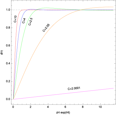
Figure 1: Stationary field configurations $f(u)$ for different values of parameter $C$.

As it is noticed in ref. BV the stationary solutions can be found only for $C>2$, but no explanation of this observation is given therein. Let us try to explain why the value $C=2$ is the special one.

From Eq. (7) and condition $f(0)=0$ it follows that $f^{\prime\prime}(0)=0$. Using this condition and expanding $f(u)$ into Taylor series near $u=0$, one obtains that for sufficiently small positive $\epsilon$ and for $f^{\prime}(0)>0$:

$$f^{\prime\prime}(\epsilon) < 0,\hskip 8.53581pt\mathrm{for}\hskip 5.69054ptC>2,\hskip 5.69054pt\mathrm{and}$$ (9)

$$f^{\prime\prime}(\epsilon) > 0,\hskip 8.53581pt\mathrm{for}\hskip 5.69054ptC\leq 2.$$ (10)

In other words, if the function $f(u)$ satisfies Eq. (7) and the boundary conditions are $f(0)=0$ and $f^{\prime}(0)>0$, then $f(u)$ is convex for $C>2$ and small positive $u$, like ordinary kink-type solution is. However, for $C\leq 2$ the function $f(u)$ is concave, therefore it can not be the kink-type one. So this is a simple explanation why in the case $C\leq 2$ there are no stationary solutions of Eq. (7) with boundary conditions (8). On the other hand, if we allow for an arbitrary dependence of the solution on $z$ and $t$, it exists for any $C$, but the case of $C\leq 2$ leads to the expanding kink with rising width, as it is shown in the next section.

A more formal proof that there are no stable solutions for $C\leq 2$ can be found in Appendix A.

III Evolution of domain walls beyond the stationary limit

As we have seen in the previous section, Eq. (7) allows to find the field configurations, which describe stationary domain walls in expanding universe. However, it is also interesting to see how domain walls evolve from some initial states. Beyond the stationary approximation we can find not only solution for $C>2$ but also for $C\leq 2$, for which the stationary approximation does not exist.

To this end one should solve the original equation of motion (3) in the case when the field $\varphi$ is a function of two independent variables, $z$ and $t$:

$$\frac{\partial^{2}\varphi}{\partial t^{2}}+3H\frac{\partial\varphi}{\partial t}-e^{-2Ht}\frac{\partial^{2}\varphi}{\partial z^{2}}=-2\lambda\varphi\left(\varphi^{2}-\eta^{2}\right).$$ (11)

It is convenient to introduce dimensionless variables $\tau=Ht$, $\zeta=Hz$ and function $f(\zeta,\tau)=\varphi(z,t)/\eta$. As a result one obtains the equation

$$\frac{\partial^{2}f}{\partial\tau^{2}}+3\frac{\partial f}{\partial\tau}-e^{-2\tau}\frac{\partial^{2}f}{\partial\zeta^{2}}=2Cf\left(1-f^{2}\right),$$ (12)

where $C=\lambda\eta^{2}/H^{2}=1/(H\delta_{0})^{2}>0$ as it was above.

The boundary conditions for the kink-type solution should be

$$f(0,\tau)=0,\hskip 14.22636ptf(\pm\infty,\tau)=\pm 1,$$ (13)

and we choose the initial configuration as the domain wall with ”natural” thickness $1/\sqrt{C}$ (with respect to dimensionless coordinate $\zeta$) and zero time derivative:

$$f(\zeta,0)=\tanh{\frac{z}{\delta_{0}}}=\tanh{\sqrt{C}\zeta},\hskip 14.22636pt\frac{\partial f(\zeta,\tau)}{\partial\tau}\biggl{|}_{\tau=0}=0.$$ (14)

Of course, this is a toy model with the artificial initial conditions. The realistic model should describe the evolution of domain walls from the very beginning, including the process of wall formation. This will be studied elsewhere.

We analyze solutions of Eq. (12) starting from large values of parameter $C$ gradually moving to smaller ones.

The evolution of the domain wall for $C=4$ is depicted in Fig. 2. The stationary solution is shown there by black curve (it is denoted by ”BV” because of Basu and Vilenkin who found it in ref. BV ). One sees that the domain wall evolves from the initial state (14) in somewhat non-trivial way. At the very beginning the wall starts to broaden in terms of the proper distance from the wall, $zH\exp{Ht}$, and at some moment it becomes wider than the stationary solution. However, afterwards the wall broadening changes to contraction, here it occurs approximately at $t\sim H^{-1}$ (but such ”beautiful” value of $t$ seems to be accidental). Finally, the wall comes to the stationary configuration after several damped oscillations around it. The oscillating behavior is expected because the field equation (12) is the oscillator type equation with respect to $\tau$ and the value of the first time derivative is chosen arbitrarily.

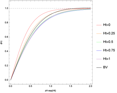
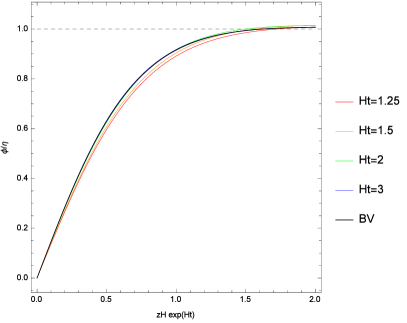
Figure 2: Evolution of domain wall for $C=4$. Black curve corresponds to stationary solution.

Let us consider now smaller values of parameter $C$. When it is close to its critical value $C=2$, the stationary domain wall is quite wide (see Fig. 1). Therefore, if the initial thickness of the wall is $1/\sqrt{C}$ (14), one should expect that the non-stationary solution approaches to the stationary one only after quite long time. The corresponding evolution of domain wall for $C=2.5$ is depicted in Fig. 3.

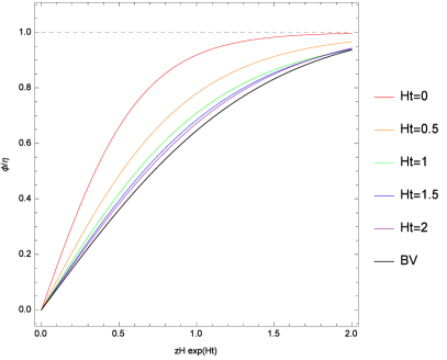
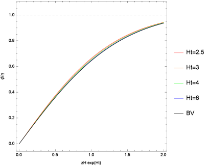
Figure 3: Evolution of domain wall for $C=2.5$. Initial configuration is $f(\zeta,0)=\tanh{\sqrt{C}\zeta}$.

It may be also interesting to choose an initial domain wall with the thickness greater than that of the stationary solution. For such case see Fig. 4, where the evolution of domain wall with initial thickness $3/\sqrt{C}$ for $C=2.5$ is presented. The wall also eventually comes to the stationary configuration.

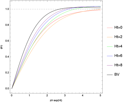
Figure 4: Evolution of domain wall for $C=2.5$. Initial configuration is $f(\zeta,0)=\tanh(\sqrt{C}\zeta/3)$.

When $C$ is very close to 2, the solution of Eq. (12) converges to the stationary one very slowly. One can see that in Fig. 5 for $C=2.05$.

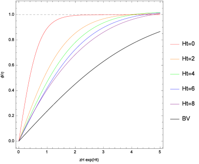
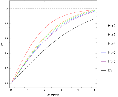
Figure 5: Evolution of domain wall for $C=2.05$. Initial configuration is $f(\zeta,0)=\tanh{(\sqrt{C}\zeta)}$ (left plot) and
$f(\zeta,0)=\tanh{(\sqrt{C}\zeta/4)}$ (right plot).

For $C\leq 2$ there are no stationary solutions at all. Evolution of domain wall for such values of parameter $C$ is shown in Fig. 6. One can see that the domain wall thickness increases indeed.

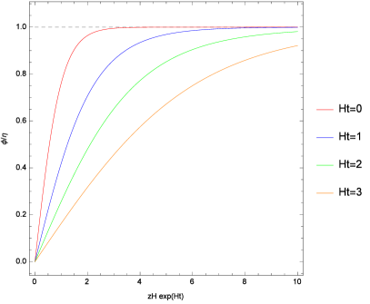
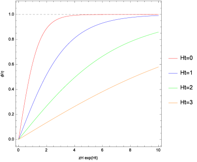
Figure 6: Evolution of domain wall for $C=1$ (left plot) and $C=0.5$ (right plot).

In an earlier paper dgrt we assumed that the size of the transition regions between baryon and antibaryon domains (such regions formed in the place of the disappeared domain walls) could be exponentially large, so the domains would be separated by a few Mpc (in the present day scale). Let us check now if this can be true and what is the proper magnitude of the parameters. So we have to calculate how fast the domain wall thickness can increase in de Sitter universe. In our model the wall is described at the initial moment by hyperbolic tangent $\varphi/\eta=\tanh{(z/\delta)}$, where the wall thickness is denoted by $\delta$. Although in the realistic course of the evolution the wall is not ”pure” hyperbolic tangent, nevertheless one can use the same definition for the thickness $\delta(t)$ as the value of the coordinate $z$ at the position where the field $\phi$ reaches the value $\phi/\eta=\tanh{1}\approx 0.76$.

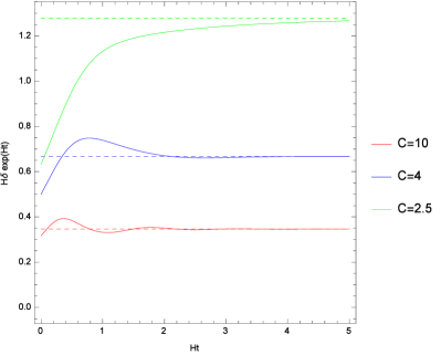
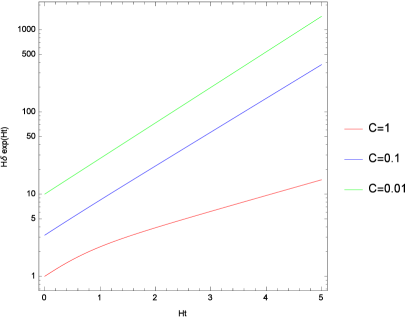
Figure 7: Time dependence of domain wall thickness for $C>2$ (left plot) and $C<2$ (right plot). Dashed lines describe the stationary solutions.

In Fig. 7 the time dependence of the physical width of the wall in dimensionless units, $H\delta\exp{Ht}$, for different values of $C$ is presented. In the left plot ($C>2$) one can see that all the curves indeed tend to constant values corresponding to stationary solutions (dashed lines). Oscillatory behavior mentioned above is also apparent. Right plot contains curves for $C<2$. Along the vertical axis the wall thickness is shown in logarithmic scale in order to compare the rate of the wall expansion with the exponential cosmological one. It is clear that for $C=1$, i.e. for not very small values of $C$, the wall thickness increases slower than exponent. However, for smaller values of $C$, e.g. $C\lesssim 0.1$ the rate of the wall expansion is the exponential one with a good accuracy.

The Hubble constant, $H$, plays the role of friction in this problem and when it dominates over the potential term ($C\ll 1$), the field configuration as a function of coordinates becomes almost static. Therefore the width of the wall is growing nearly as the scale factor $a(t)$, i.e. almost exponentially. This is why there are no stable solutions for $C\ll 1$.

IV Conclusions

Time evolution of thick domain walls in a de Sitter universe is considered. We have shown that for large values of parameter $C>2$ the initial kink configuration in a de Sitter background tends to the stationary solution obtained by Basu and Vilenkin BV . We also confirmed the BV result that the width of the stationary wall rises with decreasing value of $C$.

For $C<2$ the stationary solution does not exist and the width of the wall infinitely grows with time. For $C\lesssim 0.1$ the rise is close to the exponential one within the precision of our numerical calculations. This result confirms the assertion made in ref. dgrt that the transition region between matter and antimatter domain might be cosmologically large. This result is essential for application of spontaneous breaking of symmetry between particles and antiparticles to realistic cosmology. In our version of this scenario dgrt the walls between matter and antimatter domains dissolved and hence the huge energy density of domain walls, which was a stumbling block of the traditional approach, did not destroy isotropy and homogeneity of the universe.

Baryogenesis in our model proceeded after the double well potential returned to the ”normal” potential with the single minimum at $\chi=0$ (here $\chi$ is field which made the wall). Correspondingly the field $\chi$ started to move from the initial values $\langle\chi\rangle=\pm\eta$ to zero, so the domain walls disappeared. However, if the classical field $\chi$ did not completely relax down to zero prior to baryogenesis, it would induce $CP$-violation of different signs at different domains which in turn led to an excess of matter or antimatter in this remnants of the regions with non-zero $\chi$.

A necessary condition to make this model realistic is a sufficiently large distance between matter and antimatter domains. Otherwise the annihilation on the boundaries would create too high gamma ray background, according to ref. CdRG . The calculations presented above demonstrate that there is some range of the parameter values, namely $C=\lambda\eta^{2}/H^{2}\lesssim 0.1$, for which the width of the domain wall exponentially rises and so the distance between matter and antimatter could be large enough.

On the other hand, too wide domain walls lead to large universe regions devoid of baryons, so it might distort the observed quasi-isotropy of CMB at the angular distance above the diffusion (Silk) damping scale. However, this statement can be questioned, since the temperature contrast between baryon/antibaryon and empty regions might push the domains apart diminishing the baryon-antibaryon diffusion towards each other and this would allow for smaller separation between the domains below the diffusion damping scale. The latter problem is under investigation now.

Note added. After this paper was submitted to journal, we were informed about the paper Voronov , where the related problems were considered. We thank A.E. Kudryavtsev for this reference.

Appendix A Absence of stable solutions for $C\leq 2$

Let us assume that equation (7)

$$\left(1-u^{2}\right)f^{\prime\prime}-4uf^{\prime}+2Cf\left(1-f^{2}\right)=0$$ (15)

with the boundary conditions (8)

$$f(0)=0,\hskip 14.22636ptf(+\infty)=1$$ (16)

has a solution $f(u)$. We suppose that there is only one zero of this solution: $f(0)=0$, i.e. $f(u)>0$ for $u>0$. This assumption looks rather natural but we have not proven it. If this is still true, then due to the symmetry of eq. (15) with respect to ”parity” transformation, $u\to-u$, this zero must be at $u=0$. Accordingly the derivative $f^{\prime}(0)$ must be positive.

Let us consider the corresponding linear equation

$$\left(1-u^{2}\right)g^{\prime\prime}-4ug^{\prime}+2Cg=0$$ (17)

with the boundary conditions

$$g(0)=0,\hskip 14.22636ptg^{\prime}(0)=f^{\prime}(0)>0.$$ (18)

The solution of eq. (17) is close to $f(u)$ near $u=0$, when $f\ll 1$.

This equation can be easily solved analytically. For $C=2$ there is a special linear solution, $g(u)=f^{\prime}(0)u$, while for an arbitrary $C$ the solution is:

$$g(u)=f^{\prime}(0)\cdot u\cdot{{}_{2}F_{1}}\left(C_{5}^{-},C_{5}^{+};\frac{3}{2};u^{2}\right),$$ (19)

where ${{}_{2}F_{1}}$ is the hypergeometric function and

$$C_{n}^{\pm}\equiv\frac{n\pm\sqrt{8C+9}}{4}.$$ (20)

For $C<2$ one has $C_{5}^{\pm}>0$, therefore this hypergeometric function goes to $+\infty$ when $u\to 1$. The change in its behavior occurs when $C_{5}^{-}$ changes its sign, i.e. at $C=2$. The solutions of eq. (17) for $C<2$, $C=2$ and $C=2.1$ with boundary conditions (18) are presented in Fig. 8.

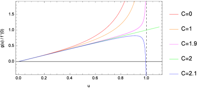
Figure 8: Solutions of equation (17) for different values of $C$.

In what follows we will show that if $C<2$, then $f(u)>g(u)$ in the interval $0<u<1$ and therefore the natural assumption that the solution $f(u)$ is positive and bounded happens to be incorrect since if $C<2$, then $g(u)\to+\infty$ when $u\to 1$ (see Fig. 8).

The difference $\Delta(u)\equiv f(u)-g(u)$ satisfies the following equation:

$$\left(1-u^{2}\right)\Delta^{\prime\prime}-4u\Delta^{\prime}+2C\Delta=h(u)\equiv 2Cf^{3}(u)$$ (21)

with the boundary conditions

$$\Delta(0)=0,\hskip 14.22636pt\Delta^{\prime}(0)=0.$$ (22)

Here we just want to verify the inequality $f(u)>g(u)$, and therefore we are interested only in the sign of $\Delta(u)$.

Since the solution of the homogeneous equation vanishes due to the boundary conditions (22), the solution of eq. (21) is given by

$$\Delta\left(u\right)=\int\limits_{0}^{+\infty}h(v)G(u,v)dv,$$ (23)

where $G(u,v)$ is the Green’s function of eq. (21). It satisfies:

$$\left(1-u^{2}\right)G^{\prime\prime}-4uG^{\prime}+2CG=\delta(u-v)$$ (24)

with boundary conditions (22). Here prime means derivative with respect to $u$ and $\delta(u-v)$ is the Dirac delta function.

The solution of (24) can be found analytically (we are interested in $G(u,v)$ only for $0<u<1$):

$$G(u,v)=\frac{3\Theta\left(u-v\right)}{\left(1-v^{2}\right)}\frac{uI\left(3;\frac{1}{2};v^{2}\right)I\left(5;\frac{3}{2};u^{2}\right)-vI\left(3;\frac{1}{2};u^{2}\right)I\left(5;\frac{3}{2};v^{2}\right)}{6Cv^{2}I\left(5;\frac{3}{2};v^{2}\right)I\left(7;\frac{3}{2};v^{2}\right)+I\left(3;\frac{1}{2};v^{2}\right)\left[3I\left(5;\frac{3}{2};v^{2}\right)+2(2-C)v^{2}I\left(9;\frac{5}{2};v^{2}\right)\right]},$$ (25)

where $\Theta(u-v)$ is the Heaviside step function and we have introduced the following notation:

$$I\left(n;c;u^{2}\right)\equiv{{}_{2}F_{1}}\left(C_{n}^{-},C_{n}^{+};c;u^{2}\right).$$ (26)

Studying the Green’s function one can find that it is non-negative, $G(u,v)\geq 0$, for $0<u<1$ and $C<2$. For the illustration of that see Fig. 9 where $G(u,v)$ as function of $v$ for a couple of different constant values of $u$ is presented. Since $h(v)\geq 0$ according to our assumption, one sees from (23) that $\Delta(u)\geq 0$ for $0<u<1$. As it was mentioned above, it proves that there are no solutions of eq. (15) for $C<2$.

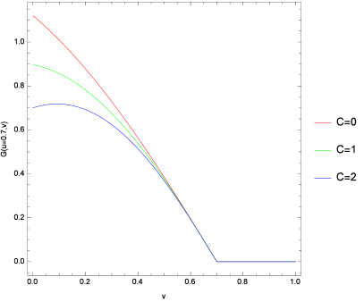
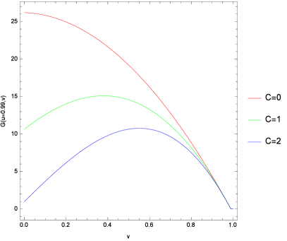
Figure 9: Green’s function $G(u,v)$ for $u=0.7$ (left) and $u=0.99$ (right).

In the case of $C=2$ it is not enough to find that $f(u)>g(u)$ since there is no singularity in $g(u)$ at $u=1$. But $G(u,v)$ itself has a positive singularity at $u=1$ for any $v>0$ (see Fig. 10). Then it follows from (23) that $\Delta(u)$ goes to $+\infty$ at $u=1$ and therefore for $C=2$ there are no stable solutions of eq. (15) as well.

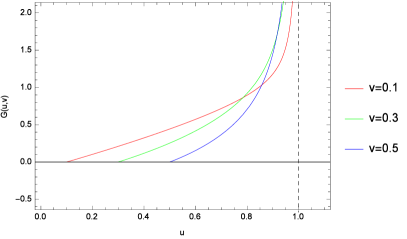
Figure 10: Green’s function $G(u,v)$ for different values of $v$ in the case $C=2$.

References

- (1) R. Basu and A. Vilenkin, Evolution of topological defects during inflation, Phys. Rev. D 50 (1994) 7150 [gr-qc/9402040].
- (2) T.D. Lee, nonconservation and spontaneous symmetry breaking, Phys. Rept. 9 (1974) 143.
- (3) Y.B. Zeldovich, I.Y. Kobzarev and L.B. Okun, Cosmological consequences of the spontaneous breakdown of discrete symmetry, Zh. Eksp. Teor. Fiz. 67 (1974) 3 [Sov. Phys. JETP 40 (1974) 1].
- (4) V.A. Kuzmin, I.I. Tkachev and M.E. Shaposhnikov, Are there domains of antimatter in the universe? (in Russian), Pisma Zh. Eksp. Teor. Fiz. 33 (1981) 557.
- (5) V.A. Kuzmin, M.E. Shaposhnikov and I.I. Tkachev, Gauge hierarchies and unusual symmetry behavior at high temperatures, Phys. Lett. B 105 (1981) 159.
- (6) V.A. Kuzmin, M.E. Shaposhnikov and I.I. Tkachev, Matter-antimatter domains in the universe: a solution of the vacuum walls problem, Phys. Lett. B 105 (1981) 167.
- (7) V.A. Kuzmin, M.E. Shaposhnikov and I.I. Tkachev, Baryon generation and unusual symmetry behavior at high temperatures, Nucl. Phys. B 196 (1982) 29 [Erratum ibid. B 202 (1982) 543].
- (8) A.D. Dolgov, S.I. Godunov, A.S. Rudenko and I.I. Tkachev, Separated matter and antimatter domains with vanishing domain walls, JCAP 10 (2015) 027 [arXiv:1506.08671].
- (9) A.D. Dolgov, Non-GUT baryogenesis, Phys. Rept. 222 (1992) 309.
- (10) A.D. Dolgov, Baryogenesis, 30 years after, Surveys High Energ. Phys. 13 (1998) 83 [hep-ph/9707419].
- (11) A.D. Dolgov, violation in cosmology, lectures given at 163rd Course of International School of Physics ’Enrico Fermi’: Violation: From Quarks to Leptons, Varenna Italy (2005) [hep-ph/0511213].
- (12) A.G. Cohen, A. De Rujula and S.L. Glashow, A matter-antimatter universe?, Astrophys. J. 495 (1998) 539 [astro-ph/9707087].
- (13) N.A. Voronov, A.L. Dyshko and N.B. Konyukhova, On the stability of a self-similar spherical bubble of a scalar Higgs field in de Sitter space, Yad. Fiz. 68 (2005) 1268 [Phys. Atom. Nucl. 68 (2005) 1218].